Selective Inference Approach for
Statistically Sound Discriminative Pattern Discovery
Abstract
Discovering statistically significant patterns from databases is an important challenging problem. The main obstacle of this problem is in the difficulty of taking into account the selection bias, i.e., the bias arising from the fact that patterns are selected from extremely large number of candidates in databases. In this paper, we introduce a new approach for predictive pattern mining problems that can address the selection bias issue. Our approach is built on a recently popularized statistical inference framework called selective inference. In selective inference, statistical inferences (such as statistical hypothesis testing) are conducted based on sampling distributions conditional on a selection event. If the selection event is characterized in a tractable way, statistical inferences can be made without minding selection bias issue. However, in pattern mining problems, it is difficult to characterize the entire selection process of mining algorithms. Our main contribution in this paper is to solve this challenging problem for a class of predictive pattern mining problems by introducing a novel algorithmic framework. We demonstrate that our approach is useful for finding statistically significant patterns from databases.
Keywords
Statistically-sound data mining; Predictive pattern mining; Selective inference; Statistical hypothesis testing
1 Introduction
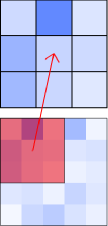
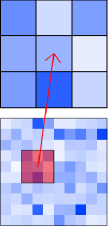
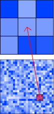
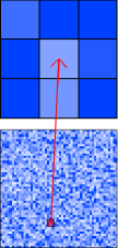
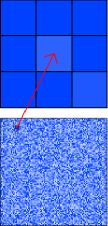
Discovering statistically reliable patterns from databases is an important challenging problem. This problem is sometimes referred to as statistically sound pattern discovery [1, 2]. In this paper we introduce a new statistically sound approach for predictive pattern mining [3, 4, 5]. Although the main goal of predictive pattern mining is to discover patterns whose occurrences are highly associated with the response, it is often desirable to additionally provide the statistical significance of the association for each of the discovered patterns (e.g., in the form of -values). However, properly evaluating the statistical significance of pattern mining results is quite challenging because the selection effect of the mining process must be taken into account. Noting that predictive pattern mining algorithms are designed to select patterns which are more associated with the response than other patterns in the database, even if all the patterns in the database have no true associations, the discovered patterns would have apparent spurious associations by the selection effect. Such a distortion of statistical analysis is often referred to as selection bias [6]. Figure 1 is a simple illustration of selection bias.
 |
 |
 |
 |
 |
|
|---|---|---|---|---|---|
| 55 | 1010 | 2525 | 5050 | 100100 |

In this paper, we introduce a new approach for solving the selection bias issue for a class of predictive pattern mining problems. Our new approach is built on a framework called selective inference (see, e.g., [7]). The main idea of selective inference is that, by considering a sample space conditional on a particular selection event, we do not have to mind the bias stemming from the selection event. In the context of pattern mining, it roughly indicates that, if we make a statistical inference (computing -values or confidence intervals etc.) based on a sampling distribution under the condition that a particular set of patterns are discovered, the selection bias of the mining algorithm could be removed.
Although the concept of selective inference has long been discussed in the statistics community, no practical selective inference frameworks have been developed until very recently [8]. The difficulty of selective inference lies in the requirement that we must be able to derive the sampling distribution of the test statistic under the condition that the selection event actually takes place. Although deriving such a sampling distribution is generally intractable, Lee et al. [9] recently proposed a practical selective inference procedure for feature selection problems in linear models. Specifically, they provided a method for computing the sampling distributions of the selected linear model parameters under the condition that a particular set of features are selected by using a certain class of feature selection algorithms.
Our main contribution in this paper is to extend the idea of Lee et al [9], and develop a selective inference procedure for a class of predictive pattern mining problems. We develop a novel method for computing the exact sampling distribution of a relevant test statistic on the discovered patterns under the condition that those patterns are discovered by using the mining algorithm. We note that this extension is non-trivial because we need to take into account extremely large number of patterns in the database. For circumventing this computational issue, we consider a tree structure among patterns and derive a novel pruning condition that enables us to efficiently identify a set of patterns which have no effect on the sampling distribution. To the best of our knowledge, this paper is the first to address selection bias issue in pattern mining via selective inference framework. The above pruning rule enables us to develop a practical selective inference framework that can be applied to a class of predictive pattern mining problems in which extremely large number of patterns are involved.
1.1 Related approaches
In most existing pattern mining procedures, the reliability of the discovered patterns are quantified by non-statistical measures such as support, confidence, lift or leverage [10]. These non-statistical measures are easy to interpret and would be sufficient for some applications. However, when the data is noisy and considered to be a random sample from the population of interest, it is desired to provide statistical significance measures such as -values or confidence intervals for each of the discovered patterns. Although several researchers in data mining community studied how to compute statistical significances of the discovered patterns [11, 12, 13, 14], the reported -values in these studies are biased in the sense that the selection effect of the mining algorithms are not taken into account (unless a multiple testing correction procedure is applied to these -values afterward).
In machine learning community, the most common approach for dealing with selection bias is data splitting. In data splitting, the dataset is divided into two disjoint sets. One of them is used for pattern discovery and the other is used for statistical inference. Since the inference phase is made independently of the discovery phase, we do not have to care about the selection effect. An obvious drawback of data splitting is that the powers are low both in discovery and inference phases. Since only a part of the dataset can be used for mining, the risk of failing to discover truly associated patterns would increase. Similarly, the power of statistical inference (i.e., the probability of true positive finding) would decrease because the inference is made with a smaller dataset. In addition, it is quite annoying that different patterns might be discovered if the dataset is split differently. It is important to note that data splitting is also regarded as a selective inference because the inference is made only for the discovered patterns in the discovery phase, and the other undiscovered patterns are ignored.
In statistics community, multiple testing correction (MTC) has been used for addressing selection bias issue [15, 16]. MTC methods have been developed for simultaneously control the false positive errors of multiple hypothesis tests (which is sometimes called simultaneous inference). For example, the most common measure for multiple hypothesis testing is family-wise error (FWE), the probability of finding one or more false positives in the multiple tests. If a MTC method assures FWE control, then the method is also valid for selection bias correction in the sense that the probability of false positive finding can be smaller than the specified significance level . A notorious drawback of MTC is that they are highly conservative when the number of tests is large, meaning that the power of inference is very low. For example, in Bonferroni correction method, one can declare a pattern to be positive only when its nominal -value is smaller than , where is the number of all possible patterns in the database [2] 111 Recently, Terada et al. [17] pointed out in pattern mining context that the denominator of the multiple testing correction can be smaller than for a certain type of statistical inferences (such as Fisher exact test) by using an idea by Tarone [18], and several subsequent works in the same direction have been presented [19, 20, 21, 22]. . Since the number of tests (i.e., the number of all possible patterns ) is extremely large, the use of a multiple testing correction usually results in very few significant pattern findings.
If we use proper selective inference method, the corrected -values (called selective -values hereafter) of the discovered patterns can be regarded as nominal -values just like they were obtained without selection. For example, if we want to control FWE within the discovered patterns, we can use Bonferroni correction just like we only had the discovered patterns from the beginning, i.e., we declare a pattern to be positive if its selective -value is less than where is the number of the discovered patterns. It is interesting to note that, when , i.e., when all the patterns in the database are discovered, the selective inference followed by Bonferroni correction approach coincides with the simultaneous inference in the previous paragraph. In many pattern mining tasks, simultaneous inference would not be necessary and selective inference would be sufficient because we are only interested in the discovered patterns, and do not care about the other patterns in the database [23]. In [2], the author suggested to use data splitting approach at first, and then apply statistical inference with Bonferroni correction for controlling FWE within the discovered patterns. His approach is similar in spirit with the above selective inference followed by Bonferroni correction approach.
1.2 Notation and outline
We use the following notations in the remainder. For any natural number , we define . A vector and a matrix is denoted such as and , respectively. The index function is written as which returns if is true, and otherwise. The sign function is written as which returns if , and otherwise. An identity matrix is denoted as .
Here is the outline of the paper. §2 presents problem formulation, illustrative example, formal description of selective inference, and a brief review of recent selective inference literature. §3 describes our main contribution, where we develop a method that enables selective inference for a class of discriminative pattern mining problems. §4 discusses extensions and generalizations. §5 covers numerical experiments for demonstrating the advantage of selective inference framework in the context of pattern discovery. §6 concludes the paper.
2 Preliminaries
In this section, we first formulate the problem considered in this paper. Although the selective inference can be similarly applied to wider class of pattern mining problems than we consider here, we study a specific predictive item-set mining problem for concreteness. Extensions and generalizations are discussed in §4. After presenting a simple illustrative example in §2.2, we formally describe selective inference framework and explain why it can be used for addressing selection bias problems in §2.3. Finally, we review a recent result on selective inference by Lee et al.[9], which is the core basis of our main contribution in §3.
2.1 Problem statement
We study predictive item-set mining problems with continuous responses [24, 25, 26, 27]. Let us consider a database with transactions, which we denote as . Each transaction consists of a subset of binary items and a response , where we assume that the latter is centered so that . We sometimes use a compact notation where and . We sometimes restrict our attention on item-sets of the sizes no greater than . The set of all those patterns is denoted as , its size as , and each pattern in as , where is the power set of . Similarly, for each transaction, the set of patterns in of the sizes no greater than is denoted as . For representing whether each pattern in is included in a transaction, we define
| (3) |
for . A vector notation is used for representing the occurrence of the -th pattern.
Consider the following concrete example for intuitive understanding of our notations:
where we have transactions and items A, B and C. If we set , patterns222Note that we do not consider an empty set as a pattern. are
Similarly, the set of patterns for each transaction are
Alternatively, the occurrence of patterns are represented by the following -by- matrix information whose -th element is :
The occurrence of each of the patterns is the column of the above matrix, i.e.,
In the statistical inference framework we discuss here, we assume that the response is a sample from a Normal distribution , where is the unknown mean that possibly depends on the occurrence of patterns in , and is the known variance. Assuming the homoscedasticity and independence, the statistical model on which the inference is made is written as
| (4) |
where .
The goal of the problem we consider here is to discover patterns that are statistically significantly associated with the response. For each pattern , we define a statistic for in order to quantify the strength of the association with the response. Noting that are centered, the statistic would have positive (resp. negative) values when the occurrence of the pattern is positively (resp. negatively) associated with the response.
For concreteness, we consider pattern mining algorithms for discovering the top patterns based on the statistic . We denote the set of indices of those discovered patterns as , i.e., . The goal of this paper is to introduce a procedure for providing the statistical significances of the associations in the form of -values for those discovered patterns in .
2.2 An illustrative example
We illustrate basic concepts of selective inference by a toy example with transactions and items. Consider a database . Since , we have patterns: , and , and the occurrence vectors of these three patterns are , and . Suppose that we select only pattern whose association , is greatest. Since , and , the second pattern would be selected here.
Consider a null hypothesis that is from . In naive statistical inference, under , the -value of the observed is given by
| (5) |
meaning that one would conclude that the association of the pattern is significant at level. In selective inference, the statistical significance is evaluated conditional on the selection event that the pattern is selected. Thus, the selective -value is given by
| (6) |
meaning that one would conclude that the association of the pattern is NOT significant at level if we consider the fact that was selected.
In order to compute selective -values in the form of (6), we need to characterize the condition in a tractable way. In this extremely simple toy example, the condition can be simply written as
| (7) |
It means that the conditional probability in (6) is rephrased as .
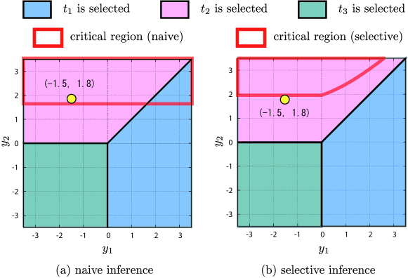
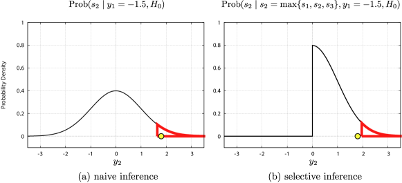
Figure 2 shows the two dimensional sample space of , where the space is divided into three regions depending on which of the three patterns , or would be selected. The problem of computing the conditional probability in (6) can be interpreted as the problem of computing the probability of conditional on an event that is observed somewhere in the pink region in Figure 2. The figure also shows critical regions in which -values in (5) or (6) are smaller than 0.05. In naive inference, is declared to be significantly large if it is greater than , where is the cumulative distribution function of . On the other hand, in selective inference, is declared to be significantly large if it is large enough even if we take into account the fact that is greater than and . Figure 3 shows the naive sampling distribution in (5) and the selective sampling distribution in (6). The critical region and the sampling distribution of selective inference in Figures 2 and 3 are obtained by using the framework we discuss later.
2.3 Selective inference
In this subsection we formally present selective inference framework in the context of predictive pattern mining problems. See [28] for a general comprehensive formulation of selective inference framework. An inference on is made conditional on its orthogonal component in the sample space (as the inference is conditioned on in the toy example in §2.2). We denote the event that the orthogonal component is as .
We consider the following two-phase procedure:
-
1.
Discovery phase: Discover a set of patterns by applying a pattern mining algorithm to the database . We denote the discovery phase as .
-
2.
Inference phase: For each discovered pattern , compute the statistical significance of the association by using a selective inference conditional on an event that the patterns are discovered.
The selective inference is conducted under the statistical model (4). In order to test the association between a discovered pattern and the response , we consider the following null hypothesis:
| (8) |
Under , we define the selective -value as
| (9) |
where the superscript (K) indicates that the selective -values are defined under the condition that the patterns are discovered in the first phase.
2.3.1 Properties of selective -values
Let us define a test as
| (12) |
Then, the probability of selective false positive error can be smaller than the significance level , i.e.,
This can be interpreted that, when a set of patterns discovered by a mining algorithm is given to a user, and the user wants to judge each of the discovered pattern to be positive or negative, the test in (12) allows the user to properly control the frequency of false positive findings.
Furthermore, if a user wants to control family-wise error of the discovered patterns, then we can apply, e.g., usual Bonferroni correction procedure, to the discovered patterns by regarding the selective -values as the nominal -values. Specifically, let for . Then, if we select the subset of the discovered patterns such that , then, we can guarantee that the probability of finding one or more false positives in is smaller than . We call as Bonferroni-adjusted selective -values in §5.
We note that, if we consider two different cases where different patterns and are discovered in the first phase, even when a pattern is discovered in both cases, the two -values and have different interpretations and cannot be compared. A key idea of selective inference is that the inference is made conditional on a single particular selection event , and other cases are never considered. It is important to remind that the goal of selective inference is not to guarantee the goodness of the mining algorithm in the first phase, but to warrant the validity of the inference in the second phase.
Another important note is about the null hypothesis in (8). When we specify the null distribution of the statistic , we do not need to specify a null distribution of itself. In other words, under any null distributions of in the form of
| (13) |
the selective -values in (9) has desired property, meaning that we do not need to specify any prior knowledge about the data generating process except (13). In the simulation study in §2.2, the null distribution is just an instance of a class of distributions in the form of (13).
2.3.2 How to compute selective -values
The main technical challenge in selective inference is how we can compute selective -values in the form of (9). To this end, we need to characterize the selection event in a tractable way. As in the toy example in §2.2, a selection event that a particular set of patterns are discovered by a mining algorithm can be interpreted as an event that the response vector is observed within a particular region in the sample space . Denoting such a region as , the above interpretation is formally stated as
Recently, Lee et al. [9] studied a class of feature selection methods in which a selection event can be represented by a set of linear inequalities in the sample space , which they call a linear selection event. In a linear selection event, the region is a polyhedron. The authors in [9] showed that, when is a polyhedron, the sampling distribution conditional on the polyhedron is a truncated normal distribution, and the truncation points are obtained by solving optimization problems over the polyhedron. For a class of feature selection problems considered in [9], it is possible to solve the optimization problems, and the selective -values can be computed with reasonable computational cost.
In §3, we see that an event of selecting the top patterns according to the association scores , can be also represented as a polyhedron in the sample space . Unfortunately, however, the polyhedron is potentially characterized by an extremely large number of linear inequalities, and it turns out to be difficult to solve the optimization problems over the polyhedron as is done in [9]. Our main contribution in this paper is to overcome this difficulty by developing a novel algorithm for efficiently identifying linear inequalities that are guaranteed to be irrelevant to the selective sampling distribution. After briefly reviewing the result of [9] in §2.4, we present selective inference framework for the pattern mining problems in §3.
2.4 Polyhedral lemma by Lee et al. [9]
In this subsection, we summarize the recent result by Lee et al. [9].
Lemma 1 (Polyhedral Lemma [9]).
Consider a linear selection event that the corresponding region is a polyhedron, and denote it as . For a statistic in the form of with an arbitrary , under a null hypothesis in the statistical model (4), the sampling distribution of conditional on a selection event can be written as
where represents the cumulative distribution function (c.d.f.) of the truncated Normal distribution which is defined by truncating the c.d.f. of a Normal distribution at , and the truncation points and are given as
| (14a) | ||||
| (14b) | ||||
The above lemma tells that the selective sampling distribution is defined by considering the frequency property of the statistic within the polyhedron , which can be characterized by solving a minimization and a maximization problems over the polyhedron in (14). Remembering that is Normally distributed, is also Normally distributed. If we restrict our attention only within the polyhedron , the distribution of is a truncated Normal distribution in which each truncation point corresponds to one of the boundaries of the polyhedron. See [9] for the proof and more detailed implications of Lemma 1.
3 Selective inference for predictive pattern mining
In this section, we introduce a selective inference procedure for the pattern mining problem described in the previous section. In §3.1, we first present the pattern mining method for the discovery phase, and discuss that a selection event by this algorithm is characterized by a set of linear inequalities in the sample space. Next, in §3.2, we present a novel method for the inference phase, in which we can efficiently handle extremely large number of patterns in the database.
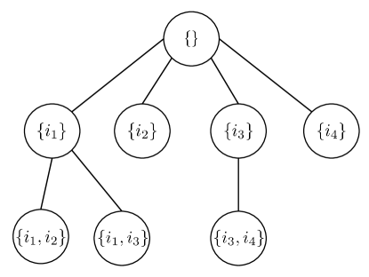
Both methods in the two phases are developed by exploiting anti-monotonicity properties defined in the item-set tree structure as depicted in Figure 4. Each node of the tree corresponds to each pattern in , and same index is used for representing a node and the corresponding pattern. For each node in the tree, we denote the set of its descendant nodes as .
3.1 Pattern mining as a linear selection event
In order to discover the top associated patterns, we develop a method searching over the item-set tree as depicted in Figure 4. In the search over the tree, we use the following pruning criterion.
Lemma 2.
Consider a node in the tree structure as depicted in Figure 4 corresponding to a pattern . Then, for any descendant node ,
| (15) |
Proof.
Noting that ,
∎
We note that Lemma 2 is not new. This simple upper bound has been used in several data mining studies such as [29, 30]. When we search over the tree, if the upper bound in (15) is smaller than the current -th largest score at a certain node , then we can quit searching over its descendant nodes .
A selection event by the above method can be characterized by a set of linear inequalities in the sample space . Noting that a fact that patterns are discovered from the database indicates that their scores , are greater than those of the other non-discovered patterns . This fact can be simply formulated as
| (16) |
Namely, a selection event by the above mining method is represented as a polyhedron defined by linear inequalities in . It indicates that, in theory, we can apply the polyhedral lemma in §2.4 to this problem. In practice, however, it is computationally intractable to naively handle all these linear inequalities.
3.2 Selective -value for pattern mining
The discussion in §3.1 suggests that it would be hard to compute selective -values in the form of (9) because the selection event is characterized by extremely large number of patterns in the database. Our basic idea for addressing this computational difficulty is to note that most of the patterns in the database actually do not affect the sampling distribution for the selective inference, and a large portion of them can be identified by exploiting the anti-monotonicity properties in the item-set trees.
Specifically, we consider item-set trees for each of the discovered patterns. Each tree consists of a set of nodes corresponding to each of the non-discovered patterns . For a pair , the -th node in the -th tree corresponds to the linear inequality in (16). When we search over these trees, we introduce a novel pruning strategy by deriving a condition such that, if the -th node in the -th tree satisfies a certain condition, then all the linear inequalities for can be ignored because they are guaranteed to be irrelevant to the sampling distribution for the selective inference, where, with a slight abuse of notation, .
Proposition 3.
The proof of Proposition 3 is presented in Appendix. This proposition indicates that the problem of computing the sampling distribution for the selective inference is reduced to the problem of searching over the trees. In the following theorem, we introduce a novel pruning condition for making the search efficient.
Theorem 4.
Consider a situation that we have already searched over some nodes in some trees, and denote them as . Furthermore, let us write the current estimates of and as and respectively.
The proof of Theorem 4 is presented in Appendix. This theorem provides explicit pruning conditions in the search process over the trees, and enables selective -value computation by making good use of the anti-monotonicity properties in the trees for efficiently identifying the patterns that are not relevant to the sampling distribution.
The pruning conditions in Theorem 4 do not depend on specific search strategies over the trees. In practice, it is more efficient to search both and simultaneously. In this case, we can develop slightly different pruning conditions that can be commonly used for the two search problems. Due to the space limitation, we do not describe the specific implementation of our search strategy.
4 Extensions
So far, we focus on a specific class of pattern mining problems described in §2.1 for concreteness. In this section, we discuss extensions.
4.1 Discovering positive and negative associations simultaneously
Previously, we have studied the problem of discovering the top positively associated patterns (or the top negatively associated patterns). It is often desired to discover the top associated patterns regardless of the signs of associations. In this case, it is natural to select the top patterns whose absolute scores are greater than the others. In this situation, it is appropriate to make inferences conditional not only on the selected patterns but also on their signs. To realize this, we slightly change the definitions of discovery event and selective -values. Let us define , i.e., the set of the discovered patterns and the signs of the associations, and write the discovery phase as . Then, in the inference phase, we define selective -values depending on the signs of the associations in the following way:
This definition is based on the idea that, if a pattern is discovered in the first step because of its high positive (resp. negative) association, we would be only interested in testing whether the positive (resp. negative) association is statistically significant or not after correcting the selection bias. By conditioning not only on the observed discovered patterns but also on the observed signs of the associations, the selection event is characterized by linear inequalities: for all .
4.2 Sequential pattern discovery
If the goal is to discover a set of patterns that are useful for predictive modeling, it is not appropriate to select patterns based only on the individual associations with the response. In this case, we should also consider correlations among the patterns because having multiple highly correlated patterns in predictive models is not very helpful. In the context of linear model learning, this problem is called feature selection, and many feature selection approaches have been studied in the literature (see, e.g., §3 in [31]). Here, we focus on a sequential pattern discovery approach in which relevant features are sequentially discovered one by one. We note that selective inference framework for sequential feature selection in linear models has been already studied in [32]. Our contribution here is again to extend it to predictive pattern mining problems by overcoming the computational difficulty in handling extremely large number of patterns in the database.
4.2.1 Discovery phase
Here, we study a sequential predictive pattern discovery method. Let be the sequence of the discovered pattern indices from step 1 to step for . Before step , we have already discovered patterns . Using these patterns, the linear predictive model is written as , where the coefficients are estimated by least-squares method. Denoting be matrix whose -th column is , the least square estimates are written as
where is the pseudo-inverse of . Then, at the step, we consider the association between the residual vector and a pattern for , and discover the one that maximizes among the patterns . Due to the space limitation, we do not describe the mining algorithm. We can develop it by using similar techniques as Lemma 2.
In the discovery phase, we thus consider a selection event that patterns and their signs are sequentially selected as described above. Namely, the selection event is written as with . At each step , an event that the feature is discovered is written as
| (20) |
for all , where . By combining all the linear selection events in steps, the entire selection event of the above sequential discovery method can be characterized by linear inequalities in . It means that, in theory, we can also apply polyhedral lemma to this sequential discovery method. In practice, however, it is computationally intractable to handle those extremely large number of linear inequalities.
4.2.2 Inference phase
In order to quantify the importance of each of the discovered patterns in the linear model, we make statistical inference on each least-square coefficient , , with being a -dimensional vector with 1 at the -th element and 0 otherwise. The null hypothesis for the -th coefficient is
Consider a polytope defined by linear inequalities in the form of (20). Then, the sampling distribution for the selective inference is a truncated Normal distribution whose truncation points are given by solving a minimization and a maximization problems over the polyhedron . Using Theorem 4, we can develop a similar algorithm for efficiently solving these optimization problems.
4.3 Mining statistically sound subgraphs
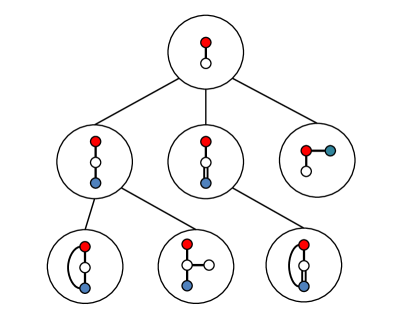
In this section, we extend the selective inference framework to graph mining problems. The goal of graph mining is to extract interesting structures from graph data, and have been demonstrated to be useful for several areas such as biology, chemistry, material science, etc [33, 34, 35, 36, 37, 26]. Here, we use selective inference framework for providing proper statistical significance measures of the extracted subgraphs obtained by graph mining algorithms. We use gSpan [38] algorithm for enumerating frequently appeared subgraphs in datasets. Figure 5 shows an illustration of a tree structure in graph mining problems.
4.3.1 Problem setup
We denote the dataset as , where is a labeled undirected graph and a response is defined on . Let be the set of all possible subgraphs in the database, and denote its size as . We denote each of the all subgraphs as , and then the occurrence of each pattern is given as the same form (3).
Note that gSpan is designed for finding subgraphs whose support (which is the number of occurrences) is grater than or equal to minimum support minsup and the maximum number of edges of subgraphs is smaller than or equal to maxpat. In this paper, we only find subgraphs which are highly associated with the response. To this end, we use the pruning condition (15) during searching subgraphs. Since the elements of are given in the same form as (3), the problem of searching those subgraphs is inherently the same as the problem of item-set mining discussed in §2.1. We can apply selective inference to graph mining problems by using the pruning conditions in Theorem 4 by exploiting the anti-monotonicity properties in the tree, although the number of all subgraphs is extremely large.
5 Experiments
5.1 Experiments on synthetic data (itemset mining)
First, we compared selective inference (select) with naive (naive) and data-splitting (split) on synthetic data. In naive, the nominal -values of the discovered patterns were naively computed without any selection bias correction mechanisms. In split, the data was first divided into two equally sized sets, and one of them was used for pattern discovery, and the other was used for computing -values. Note that the errors controlled by these methods are individual false positive rate for each of the discovered patterns (although naive actually cannot control it), we applied Bonferroni correction within the discovered patterns, i.e., we regard a pattern to be positive if the Bonferroni-adjusted selective -values (obtained by multiplying selective -values by ; see §2.3.1) is still smaller than the significance level . We only considered the problems of finding the top associated patterns regardless of the signs of associations (the setup described in §4.1). We investigated the results of two scenarios: one for finding individual associations (indicated as individual) and another for finding correlated associations by the sequential method in §4.2 (indicated as sequential).
The synthetic data was generated as follows. In the experiments for comparing false positive rates, we generated the item-set and the response independently at random for each . The item-set was randomly generated so that it contains items on average, where is an experimental parameter for representing the sparsity of the data. On the other hand, the response was randomly generated from a Normal distribution . In the experiments for comparing true positive rates, the response was randomly generated from a Normal distribution , where in individual scenario, while in sequential scenario. We investigated the performances by changing various experimental parameters. We set the baseline parameters as , , , , , , and .
5.1.1 False positive rates
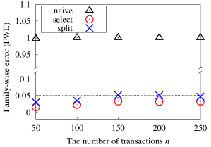
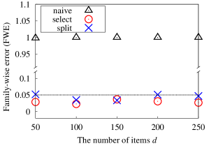
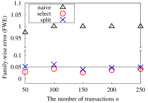
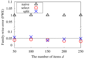
Figure 6 shows the false positive rates when varying the number of transactions , the number of items . In all cases, the FW-FPRs of naive were far greater than the desired significance level , indicating that the selection bias is harmful. The FW-FPRs of the other two approaches select and split were successfully controlled.
 |
 |
| (a) | (b) |
| individual scenario | |
 |
 |
| (c) | (d) |
| sequential scenario | |
5.1.2 True positive rates
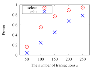
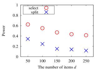
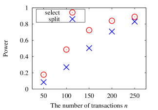
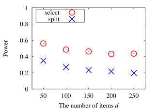
Figure 7 shows the true positive rates (TPRs) of select and split (we omit naive because it cannot control FPRs). Here, TPRs are defined as the probability of discovering truly associated item-sets. In all experimental setups, the TPRs of select were much greater than split. Note that the performances of split would be worse than select both in the discovery and the inference phases. The risk of failing to discover truly associated patterns in split would be higher than select because only half of the data would be used in the discovery phase. Similarly, the statistical power of the inference in split would be smaller than select because the sample size is smaller.
 |
 |
| (a) | (b) |
| individual scenario | |
 |
 |
| (c) | (d) |
| sequential scenario | |
5.1.3 Computational efficiency
Table 1 shows the computation times in seconds for the selective inference approach with and without the computational tricks described in §3 for various values of the number of transactions , the number of items , and the sparsity rates (we terminated the search if the time exceeds 1 day). It can be observed from the table that, if we use the computational trick, the selective inferences can be conducted with reasonable computational costs except for and cases in sequential scenario. When the computational trick was not used, the cost was extremely large. Especially when the number of items is larger than 100, we could not complete the search within 1 day. From the results, we conclude that computational trick described in §3 is indispensable for selective inferences in pattern mining problems.
| individual scenario | sequential scenario | |||||||||||||||||||||||||||||||||||||||||||||||||||||||||||||||
|---|---|---|---|---|---|---|---|---|---|---|---|---|---|---|---|---|---|---|---|---|---|---|---|---|---|---|---|---|---|---|---|---|---|---|---|---|---|---|---|---|---|---|---|---|---|---|---|---|---|---|---|---|---|---|---|---|---|---|---|---|---|---|---|---|
|
|
|||||||||||||||||||||||||||||||||||||||||||||||||||||||||||||||
|
|
|||||||||||||||||||||||||||||||||||||||||||||||||||||||||||||||
5.2 Application to HIV drug resistance data (itemset mining)
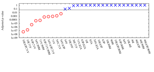
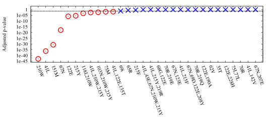
We applied the selective inference approach to HIV-1 sequence data obtained from Stanford HIV Drug Resistance Database [39]. The goal here is to find statistically significant high-order interactions of multiple mutations (up to order interactions) that are highly associated with drug resistances. Same datasets were also studied in [40]. We discovered patterns, and evaluated the statistical significances of these patterns by selective inference. Table 2 shows the numbers of 1st, 2nd, 3rd and 4th order interactions that were statistically significant in the sense that the Bonferroni adjusted selective -values is smaller than (there were no statistically significant 5th order interactions). Figure 8 shows the list of Bonferroni-adjusted selective -values in increasing order on idv and d4t datasets in individual and sequential scenario, respectively. These results indicate that selective inference approach could successfully identify statistically significant high-order interactions of multiple mutations.
| individual scenario | sequential scenario | |||||||||
| Data | | | | | Time[s] | | | | | Time[s] |
| NNRTI () | ||||||||||
| dlv() | 1 | .495 | 2 | 18.0 | ||||||
| efv() | .732 | 5 | 13.7 | |||||||
| nvp() | 4 | 1 | .774 | 8 | 17.4 | |||||
| NRTI () | ||||||||||
| 3tc() | 1 | 2 | .257 | 4 | 15.1 | |||||
| abc() | 5 | 13 | 7 | 2 | .238 | 9 | 11.7 | |||
| azt() | 2 | 5 | 3 | 1 | .231 | 5 | 17.5 | |||
| d4t() | 4 | 11 | 6 | 1 | .215 | 7 | 1 | 3 | 13.7 | |
| ddi() | 2 | 1 | .234 | 6 | 12.1 | |||||
| tdf() | .230 | 3 | 1 | 26.4 | ||||||
| PI () | ||||||||||
| apv() | 3 | 6 | 1 | .188 | 9 | 6.5 | ||||
| atv() | 1 | 3 | 2 | .150 | 3 | 1 | 5.0 | |||
| idv() | 1 | 6 | 3 | .437 | 9 | 6.2 | ||||
| lpv() | 4 | 4 | 1 | .275 | 11 | 6.1 | ||||
| nfv() | 5 | 7 | 1 | .455 | 15 | 5.8 | ||||
| rtv() | 5 | 7 | 2 | .183 | 10 | 1 | 5.6 | |||
| sqv() | 1 | 3 | 2 | .623 | 7 | 1 | 7.8 | |||
(a) idv dataset (individual scenario)
(b) d4t dataset (sequential scenario)
5.3 Experiments on graph mining with chemical data
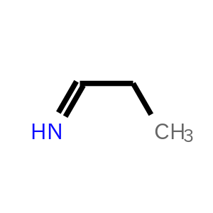
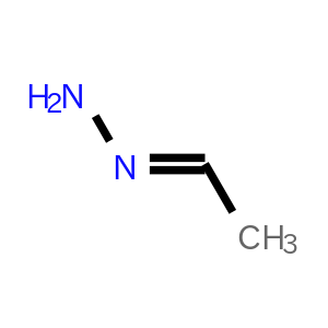
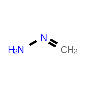
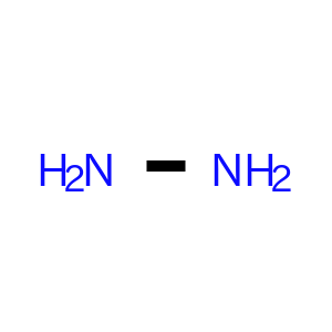
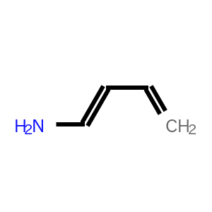
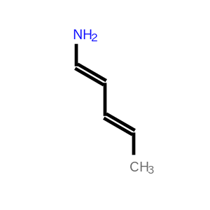
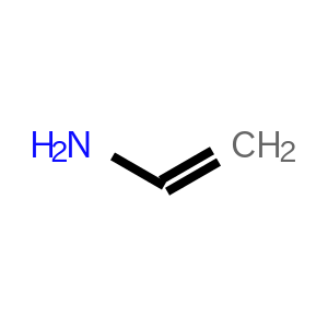
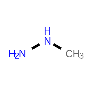
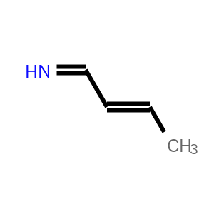
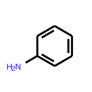
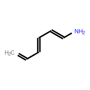
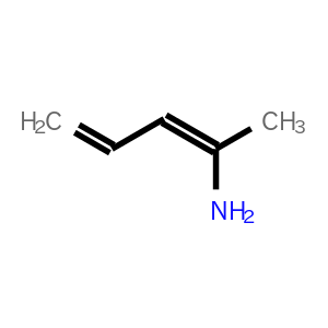
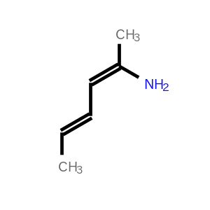
Here we used Karthikeyan dataset where the response is the melting point of each of the chemical compounds (this data is available at http://cheminformatics.org/datasets/). We considered the case with which indicates the maximum number of edges of subgraphs we wanted to find. We discovered = 50 subgraphs which are individually associated with the melting point, and evaluated the statistical significances of those subgraphs by selective inference. Table 3 shows the numbers of subgraphs that were statistically significant in the sense that the Bonferroni adjusted selective -values are smaller than , where the identified subgraphs contain up to 7 edges (there were no statistically significant subgraphs that have more than 7 edges). Figure 9 shows the list of 20 subgraphs and Bonferroni-adjusted selective -values in increasing order. These results indicate that selective inference approach could identify statistically significant subgraphs at reasonable computational costs.
| Time[s] | |||||||
|---|---|---|---|---|---|---|---|
| 3 | 5 | 7 | 7 | 8 | 6 | 1 | 5.4 |
 |
 |
 |
 |
 |
 |
 |
 |
 |
 |
 |
 |
 |
 |
 |
 |
 |
 |
 |
 |
6 Conclusion
In this paper we extended selective inference framework to predictive pattern mining problems by introducing a novel computational trick for computing selective sampling distribution for a class of mining algorithms. We demonstrate that selective inference approach is useful for finding statistically sound patterns from databases because it allows us to address selection bias issue.
References
- [1] W. Hämäläinen and G. Webb, “Statistically sound pattern discovery,” in Tutorial of the 20th ACM SIGKDD international conference on Knowledge discovery and data mining. ACM, 2014.
- [2] G. I. Webb, “Discovering significant patterns,” Machine Learning, vol. 68, no. 1, pp. 1–33, 2007.
- [3] W. Fan, K. Zhang, H. Cheng, J. Gao, X. Yan, J. Han, P. Yu, and O. Verscheure, “Direct mining of discriminative and essential frequent patterns via model-based search tree,” in Proceedings of the 14th ACM SIGKDD international conference on Knowledge discovery and data mining. ACM, 2008, pp. 230–238.
- [4] P. K. Novak, N. Lavrač, and G. I. Webb, “Supervised descriptive rule discovery: A unifying survey of contrast set, emerging pattern and subgroup mining,” The Journal of Machine Learning Research, vol. 10, pp. 377–403, 2009.
- [5] A. Zimmermann and S. Nijssen, “Supervised pattern mining and applications to classification,” in Frequent Pattern Mining. Springer, 2014, pp. 425–442.
- [6] J. J. Heckman, “Sample selection bias as a specification error,” Econometrica: Journal of the econometric society, pp. 153–161, 1979.
- [7] J. Taylor and R. J. Tibshirani, “Statistical learning and selective inference,” Proceedings of the National Academy of Sciences, vol. 112, no. 25, pp. 7629–7634, 2015.
- [8] R. Berk, L. Brown, A. Buja, K. Zhang, L. Zhao et al., “Valid post-selection inference,” The Annals of Statistics, vol. 41, no. 2, pp. 802–837, 2013.
- [9] J. D. Lee, D. L. Sun, Y. Sun, and J. E. Taylor, “Exact post-selection inference with the lasso,” arXiv preprint arXiv:1311.6238, 2013.
- [10] R. Agrawal, T. Imieliński, and A. Swami, “Mining association rules between sets of items in large databases,” in ACM SIGMOD Record, vol. 22, no. 2. ACM, 1993, pp. 207–216.
- [11] S. D. Bay and M. J. Pazzani, “Detecting group differences: Mining contrast sets,” Data Mining and Knowledge Discovery, vol. 5, no. 3, pp. 213–246, 2001.
- [12] X. Yan, H. Cheng, J. Han, and P. S. Yu, “Mining significant graph patterns by leap search,” in Proceedings of the 2008 ACM SIGMOD international conference on Management of data. ACM, 2008, pp. 433–444.
- [13] W. Hämäläinen, “Statapriori: an efficient algorithm for searching statistically significant association rules,” Knowledge and information systems, vol. 23, no. 3, pp. 373–399, 2010.
- [14] A. Arora, M. Sachan, and A. Bhattacharya, “Mining statistically significant connected subgraphs in vertex labeled graphs,” in Proceedings of the 2014 ACM SIGMOD international conference on Management of data. ACM, 2014, pp. 1003–1014.
- [15] J. P. Shaffer, “Multiple hypothesis testing,” Annual review of psychology, vol. 46, no. 1, pp. 561–584, 1995.
- [16] D. D. Jensen and P. R. Cohen, “Multiple comparisons in induction algorithms,” Machine Learning, vol. 38, no. 3, pp. 309–338, 2000.
- [17] A. Terada, M. Okada-Hatakeyama, K. Tsuda, and J. Sese, “Statistical significance of combinatorial regulations,” Proceedings of the National Academy of Sciences, vol. 110, no. 32, pp. 12 996–13 001, 2013.
- [18] R. Tarone, “A modified bonferroni method for discrete data,” Biometrics, pp. 515–522, 1990.
- [19] A. Terada, K. Tsuda, and J. Sese, “Fast westfall-young permutation procedure for combinatorial regulation discovery,” in Bioinformatics and Biomedicine (BIBM), 2013 IEEE International Conference on. IEEE, 2013, pp. 153–158.
- [20] S.-i. Minato, T. Uno, K. Tsuda, A. Terada, and J. Sese, “A fast method of statistical assessment for combinatorial hypotheses based on frequent itemset enumeration,” in Machine Learning and Knowledge Discovery in Databases. Springer, 2014, pp. 422–436.
- [21] M. Sugiyama, F. L. López, N. Kasenburg, and K. M. Borgwardt, “Significant subgraph mining with multiple testing correction,” in Proceedings of the 2015 SIAM International Conference on Data Mining, 2015, pp. 37–45.
- [22] F. L. López, M. Sugiyama, L. Papaxanthos, and K. M. Borgwardt, “Fast and memory-efficient significant pattern mining via permutation testing,” Proceedings of the 21st ACM SIGKDD Conference on Knowledge Discovery and Data Mining, 2015.
- [23] Y. Benjamini, “Simultaneous and selective inference: current successes and future challenges,” Biometrical Journal, vol. 52, no. 6, pp. 708–721, 2010.
- [24] M. Deshpande, M. Kuramochi, N. Wale, and G. Karypis, “Frequent substructure-based approaches for classifying chemical compounds,” IEEE Transactions on Knowledge and Data Engineering, vol. 17, no. 8, pp. 1036–1050, 2005.
- [25] H. Saigo, N. Krämer, and K. Tsuda, “Partial least squares regression for graph mining,” in Proceedings of the 14th ACM SIGKDD international conference on Knowledge discovery and data mining. ACM, 2008, pp. 578–586.
- [26] H. Saigo, S. Nowozin, T. Kadowaki, T. Kudo, and K. Tsuda, “gboost: a mathematical programming approach to graph classification and regression,” Machine Learning, vol. 75, no. 1, pp. 69–89, 2009.
- [27] N. S. Ketkar, L. B. Holder, and D. J. Cook, “gregress: Extracting features from graph transactions for regression,” in Twenty-First International Joint Conference on Artificial Intelligence, 2009.
- [28] W. Fithian, D. Sun, and J. Taylor, “Optimal inference after model selection,” arXiv preprint arXiv:1410.2597, 2014.
- [29] T. Kudo, E. Maeda, and Y. Matsumoto, “An application of boosting to graph classification,” in Advances in neural information processing systems, 2004, pp. 729–736.
- [30] K. Nakagawa, S. Suzumura, M. Karasuyama, K. Tsuda, and I. Takeuchi, “Safe pattern pruning: an efficient approach for predictive pattern mining,” 2016, unpublished manuscript.
- [31] J. Friedman, T. Hastie, and R. Tibshirani, The elements of statistical learning. Springer series in statistics Springer, Berlin, 2001, vol. 1.
- [32] J. D. Lee and J. E. Taylor, “Exact post model selection inference for marginal screening,” in Advances in Neural Information Processing Systems, 2014, pp. 136–144.
- [33] I. Takigawa and H. Mamitsuka, “Graph mining: procedure, application to drug discovery and recent advances,” Drug discovery today, vol. 18, no. 1, pp. 50–57, 2013.
- [34] J. Han, M. Kamber, and J. Pei, Data Mining: Concepts and Techniques, 2nd ed. Morgan Kaufmann, 2006.
- [35] A. Lancichinetti, F. Radicchi, J. J. Ramasco, S. Fortunato et al., “Finding statistically significant communities in networks,” PloS one, vol. 6, no. 4, p. e18961, 2011.
- [36] N. Weill and D. Rognan, “Development and validation of a novel protein- ligand fingerprint to mine chemogenomic space: application to g protein-coupled receptors and their ligands,” Journal of chemical information and modeling, vol. 49, no. 4, pp. 1049–1062, 2009.
- [37] C. Borgelt and M. R. Berthold, “Mining molecular fragments: Finding relevant substructures of molecules,” in Data Mining, 2002. ICDM 2003. Proceedings. 2002 IEEE International Conference on. IEEE, 2002, pp. 51–58.
- [38] X. Yan and J. Han, “gspan: Graph-based substructure pattern mining,” in Data Mining, 2002. ICDM 2003. Proceedings. 2002 IEEE International Conference on. IEEE, 2002, pp. 721–724.
- [39] S.-Y. Rhee, M. J. Gonzales, R. Kantor, B. J. Betts, J. Ravela, and R. W. Shafer, “Human immunodeficiency virus reverse transcriptase and protease sequence database,” Nucleic acids research, vol. 31, no. 1, pp. 298–303, 2003.
- [40] H. Saigo, T. Uno, and K. Tsuda, “Mining complex genotypic features for predicting hiv-1 drug resistance,” Bioinformatics, vol. 23, no. 18, pp. 2455–2462, 2007.
Appendix A Proofs
Proof of Proposition 3
Proof.
From (16), the constraint is written as
| (21a) | |||
| (21b) | |||
for all possible pairs of . (i) First, for such that , the minimum possible feasible would be
and the maximum possible feasible would be . (ii) Similarly, for such that , the minimum possible feasible would be and the maximum possible feasible would be
Since the requirements in (i) and (ii) must be satisfied for all possible , by combining (i) and (ii), and are given by (17a) and (17b), respectively. ∎
Proof of Theorem 4
Proof.
Noting that , for any descendant node
| (22a) | ||||
| (22b) | ||||
We prove the first half of the theorem. (i) From (22b),
Also from Proposition 3, any pairs such that are irrelevant to the solution . It means that, when (18) holds, for do not affect the solution of (17a). (ii) From Proposition 3, we only need to consider the case where and . When , from (22a),
It means that, when (19) holds, for do not affect the solution of (17a). By combining (i) and (ii), the first half of the theorem is proved. The latter half of the theorem can be shown similarly. ∎