Secure Approximation Guarantee for
Cryptographically Private Empirical Risk Minimization

Abstract

Privacy concern has been increasingly important in many machine learning (ML) problems. We study empirical risk minimization (ERM) problems under secure multi-party computation (MPC) frameworks. Main technical tools for MPC have been developed based on cryptography. One of limitations in current cryptographically private ML is that it is computationally intractable to evaluate non-linear functions such as logarithmic functions or exponential functions. Therefore, for a class of ERM problems such as logistic regression in which non-linear function evaluations are required, one can only obtain approximate solutions. In this paper, we introduce a novel cryptographically private tool called secure approximation guarantee (SAG) method. The key property of SAG method is that, given an arbitrary approximate solution, it can provide a non-probabilistic assumption-free bound on the approximation quality under cryptographically secure computation framework. We demonstrate the benefit of the SAG method by applying it to several problems including a practical privacy-preserving data analysis task on genomic and clinical information.

1 Introduction

Privacy preservation has been increasingly important in many machine learning (ML) tasks. In this paper, we consider empirical risk minimizations (ERMs) when the data is distributed among multiple parties, and these parties are unwilling to share their data to other parties. For example, if two parties have different sets of features for the same group of people, they might want to combine these two datasets for more accurate predictive model building. On the other hand, due to privacy concerns or legal regulations, these two parties might want to keep their own data private. The problem of learning from multiple confidential databases have been studied under the name of secure multi-party computation (secure MPC). This paper is motivated by our recent secure MPC project on genomic and clinical data. Our task is to develop a model for predicting the risk of a disease based on genomic and clinical information of potential patients. The difficulty of this problem is that genomic information were collected in a research institute, while clinical information were collected in a hospital, and both institutes do not want to share their data to others. However, since the risk of the disease is dependent both on genomic and clinical features, it is quite valuable to use both types of information for the risk modeling.

Various tools for secure MPC have been taken from cryptography, and privacy-preserving ML approaches based on cryptographic techniques have been called cryptographically private ML. A key building block of cryptographically private ML is homomorphic encryption by which sum or product of two encrypted values can be evaluated without decryption. Many cryptographically private ML algorithms have been developed, e.g., for linear regression [1, 2] and SVM [3, 4] by using homomorphic encryption property. One of limitations in current cryptographically private ML is that it is computationally intractable to evaluate non-linear functions such as logarithmic functions or exponential functions in homomorphic encryption framework. Since non-linear function evaluations are required in many fundamental statistical analyses such as logistic regression, it is crucially important to develop a method that can alleviate this computational bottleneck. One way to circumvent this issue is to approximate non-linear functions. For example, in Nardi et al.’s work [5] for secure logistic regression, the authors proposed to approximate a logistic function by sum of step functions, which can be computed under secure computation framework.

Due to the very nature of MPC, even after the final solution is obtained, the users are not allowed to access to private data. When the resulting solution is an approximation, it is important for the users to be able to check its approximation quality. Unfortunately, most existing cryptographically private ML method does not have such an approximation guarantee mechanism. Although a probabilistic approximation guarantee was provided in the aforementioned secure logistic regression study [5], the approximation bound derived in that work depends on the unknown true solution, meaning that the users cannot make sure how much they can trust the approximate solution.

The goal of this paper is to develop a practical method for secure computations of ERM problems. To this end, we introduce a novel secure computation technique called secure approximation guarantee (SAG) method. Given an arbitrary approximate solution of an ERM problem, the SAG method provides non-probabilistic assumption-free bounds on how far the approximate solution is away from the true solution. A key difference of our approach with existing ones is that our approximation bound is not for theoretical justification of an approximation algorithm itself, but for practical decision making based on a given approximate solution. Our approximation bound can be obtained without any information about the true solution, and it can be computed with a reasonable computational cost under secure computation framework, i.e., without the risk of disclosing private information.

The proposed SAG method can provide non-probabilistic bounds on a quantity depending on the true solution of the ERM problem under cryptographically secure computation framework, which is valuable for making decisions when only an approximate solution is available. In order to develop the SAG method, we introduce two novel technical contributions in this paper. We first introduce a novel algorithmic framework for computing approximation guarantee that can be applied to a class of ERM problems whose loss function is non-linear and its secure evaluation is difficult. In this framework, we use a pair of surrogate loss functions that bounds the non-linear loss function from below and above. Our second contribution is to implement these surrogate loss functions by piecewise-linear functions, and show that they can be cryptographically securely computed. Furthermore, we empirically demonstrate that the bounds obtained by the SAG method is much tighter than the bounds in Nardi et al.’s method [5] despite the former is non-probabilistic and assumption-free. Figure 1 is an illustration of the SAG method in a simple logistic regression example.

In machine learning literature, significant amount of works on differential privacy [6] have been recently studied. The objective of differential privacy is to disclose an information from confidential database without taking a risk of revealing private information in the database, and random perturbation is main technical tool for protecting differential privacy. We note that the privacy concern studied in this paper is rather different from those in differential privacy. Although it would be interesting to study how the latter type of privacy concerns can be handled with the approach we discussed here, we would focus in this paper on privacy regarding cryptographically private ML.

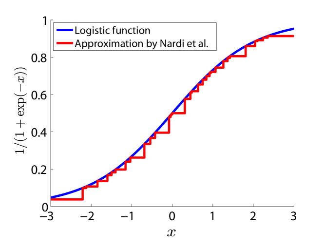(A) A non-linear function $1/(1+\exp(-x))$ and its approximation with [5]

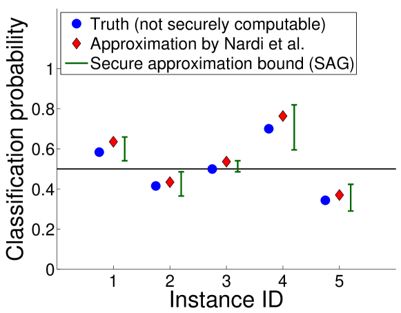(B) Class probabilities by true and approximate solutions and the bounds obtained by the SAG method.

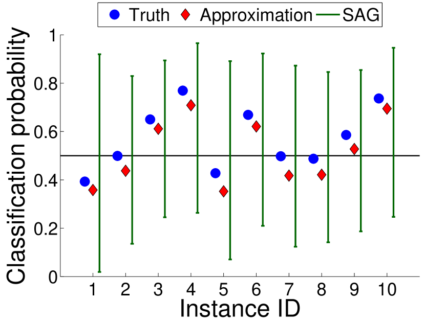
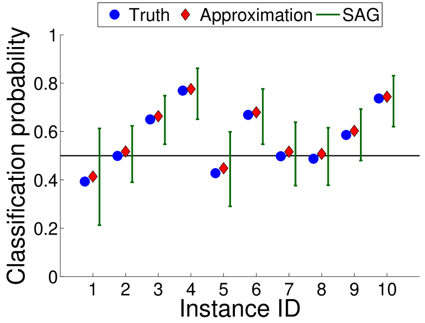
The left plot (A) shows the logistic function (blue) and its approximation (red) proposed in [5]. The right plot (B) shows the true (blue) and approximate (red) class probabilities of five training instances (the instance IDs $1,\ldots,5$ are shown in the horizontal axis), where the former is obtained with true logistic function, while the latter is obtained with the approximate logistic function.

The green intervals in plot (B) are the approximation guarantee intervals provided by the SAG method. The key property of the SAG method is that these intervals are guaranteed to contain the true class probabilities. Thus they can be used for certainly classifying some of these five instances to either positive or negative class.

Noting that the lower bounds of the class probabilities are greater than 0.5 in the instances 1 and 4, they would be certainly classified to positive class. Similarly, noting that the upper bounds of the class probabilities are smaller than 0.5 in the instances 3 and 5, they would be certainly classified to negative class.

Figure 1: An illustration of the proposed SAG method in a simple logistic regression example

Notations

We use the following notations in the rest of the paper. We denote the sets of real numbers and integers as $\mathbb{R}$ and $\mathbb{Z}$, respectively. For a natural number $N$, we define $[N]:=\{1,2,\ldots,N\}$ and $\mathbb{Z}_{N}:=\{0,1,\ldots,N-1\}$. The Euclidean norm is written as $\|\cdot\|$. Indicator function is written as $I_{\chi}$ i.e., $I_{\chi}=1$ if $\chi$ is true, and $I_{\chi}=0$ otherwise. For a protocol $\Pi$ between two parties, we use the notation $\Pi({\cal I}_{A},{\cal I}_{B})\to({\cal O}_{A},{\cal O}_{B})$, where ${\cal I}_{A}$ and ${\cal I}_{B}$ are inputs from the parties A and B, respectively, and ${\cal O}_{A}$ and ${\cal O}_{B}$ are outputs given to A and B, respectively.

2 Preliminaries

2.1 Problem statement

Empirical risk minimization (ERM)

Let $\{(\bm{x}_{i},y_{i})\in{\cal X}\times{\cal Y}\}_{i\in[n]}$ be the training set, where the input domain ${\cal X}\subset\mathbb{R}^{d}$ is a compact region in $\mathbb{R}^{d}$, and the output domain ${\cal Y}$ is $\{-1,+1\}$ in classification problems and $\mathbb{R}$ in regression problems. In this paper, we consider the following class of empirical risk minimization problems:

$$\mathop{\rm argmin}\limits_{\bm{w}}~{}\frac{\lambda}{2}\|\bm{w}\|^{2}+\frac{1}{n}\sum_{i\in[n]}\ell(y_{i},\bm{x}_{i}^{\top}\bm{w}),$$ (1)

where $\ell$ is a loss function subdifferentiable and convex with respect to $\bm{w}$, and $\lambda>0$ is the regularization parameter. $L_{2}$ regularization in (1) ensures that the solution $\bm{w}$ is within a compact region ${\mathcal{W}}\subset\mathbb{R}^{d}$.

We consider the cases where $\ell$ is hard to compute in secure computation framework, i.e., $\ell$ includes non-linear functions such as $\log$ and $\exp$. Popular examples includes logistic regression

$$\ell(y,\bm{x}^{\top}\bm{w}):=\log(1+\exp(-\bm{x}^{\top}\bm{w}))-y\bm{x}^{\top}\bm{w},$$ (2)

Poisson regression

$$\ell(y,\bm{x}^{\top}\bm{w}):=\exp(\bm{x}^{\top}\bm{w})-y\bm{x}^{\top}\bm{w},$$ (3)

and exponential regression

$$\ell(y,\bm{x}^{\top}\bm{w}):=(y\exp(-\bm{x}^{\top}\bm{w}))-\bm{x}^{\top}\bm{w}.$$ (4)

Secure two-party computation

We consider secure two-party computation scenario where the training set $\{(\bm{x}_{i},y_{i})\}_{i\in[n]}$ is vertically-partitioned between two parties A and B [7], i.e., A and B own different sets of features for common set of $n$ instances. More precisely, let party A own the first $d_{A}$ features and party B own the last $d_{B}$ features, i.e., $d_{A}+d_{B}=d$. We consider a scenario where the labels $\{y_{i}\}_{i\in[n]}$ are also owned by either party, and we let party B own them here. We assume that both parties can identify the instance index $i\in[n]$, i.e., it is possible for both parties to make communications with respect to a specified instance. We denote the input data matrix owned by parties A and B as $X_{A}$ and $X_{B}$, respectively. Furthermore, we denote the $n$-dimensional vector of the labels as $\bm{y}:=[y_{1},\ldots,y_{n}]^{\top}$.

Semi-honest model

In this paper, we develop the SAG method so that it is secure (meaning that private data is not revealed to the other party) under the semi-honest model [8]. In this security model, any parties are allowed to guess other party’s data as long as they follow the specified protocol. In other words, we assume that all the parties do not modify the specified protocol. The semi-honest model is standard security model in cryptographically private ML.

2.2 Cryptographically Secure Computation

Paillier cryptosystem

For secure computations, we use Paillier cryptosystem [9] as an additive homomorphic encryption tool, i.e., we can obtain $E(a+b)$ from $E(a)$ and $E(b)$ without decryption, where $a$ and $b$ are plaintexts and $E(\cdot)$ is the encryption function. Paillier cryptosystem has the semantic security [10] (the IND-CPA security), which roughly means that it is difficult to judge whether $a=b$ or $a\neq b$ by knowing $E(a)$ and $E(b)$.

Paillier cryptosystem is a public key cryptosystem with additive homomorphism over $\mathbb{Z}_{N}$ (i.e., ${\rm mod}N$). In public key cryptosystem, the private key is two large prime numbers $p$ and $q$, and the public key is $(N,g)\in\mathbb{Z}\times\mathbb{Z}_{N^{2}}$, where $N=pq$ and $g$ is an integer co-prime with $N^{2}$. Given a plaintext $m\in\mathbb{Z}_{N}$, a ciphertext of $E(m)$ is obtained with a random integer $R\in\mathbb{Z}_{N}$ as follows:

$$E(m)=g^{m}R^{N}\mod N^{2}.$$

Ciphertext $E(m)$ is decrypted with the private key whatever $R$ is chosen. With the encryption, the following additive homomorphism holds for any plaintexts $a,b\in\mathbb{Z}_{N}$:

$$E(a)\cdot E(b)=E(a+b),$$

$$E(a)^{b}=E(ab).$$

Hereafter, we denote by $E_{pk_{A}}(\cdot)$ and $E_{pk_{B}}(\cdot)$ the encryption functions with the public keys issued by party A and B, respectively.

Note that we need computations of real numbers rather than integers in data analysis tasks. First, negative numbers can be treated with the similar technique to the two’s complement. In order to handle real numbers, we multiply a magnification constant $M$ for each input real number for expressing it with an integer. Here, there is a tradeoff between the accuracy and range of acceptable real number, i.e., for large $M$, accuracy would be high, but only possible to handle a limited range of real numbers.

2.3 Related works

The most general framework for cryptographically private ML is the Yao’s garbled circuit [11], where any desired secure computation is expressed as an electronic circuit with encrypted components. In principle, Yao’s garbled circuit can evaluate any function securely, but its computational costs are usually extremely large. Unfortunately, it is impractical to use Yao’s garbled circuit for secure computations of ERM problems.

Nardi et al. [5] studied cryptographically private approach for logistic regression. As briefly mentioned in §1, in order to circumvent the difficulty of secure non-linear function evaluations, the authors proposed to approximate logistic function by empirical cumulative density function (CDF) of logistic distributions (see Figure 1(A) as an example). Denoting the true solution and the approximate solution as $\bm{w}^{*}$ and $\hat{\bm{w}}$, respectively, the authors showed that

$$\|\bm{w}^{*}-\hat{\bm{w}}\|\leq\frac{nc_{1}\max\|\bm{x}_{i}\|}{L^{\gamma}\lambda_{\rm min}} \text{\quad in probability~{}}1-2\exp(-cL^{1-2\gamma}),$$ (5)

where $L$ is the sample size for the empirical CDF, $\lambda_{\rm min}$ is the smallest eigenvalue of Fisher information matrix depending on $\bm{w}^{*}$, and $c>0$, $c_{1}>0$, $\gamma\in(0,1/2)$ are constants. This approximation error bound cannot be used for knowing the approximation quality of the given approximate solution $\hat{\bm{w}}$: the bound depends on the unknown true solution $\bm{w}^{*}$ because $\lambda_{\rm min}$ depends on it. Furthermore, in experiment section, we demonstrate that the SAG method can provide much tighter non-probabilistic bounds than the above probabilistic bound in Nardi et al.’s method [5].

3 Secure Approximation Guarantee(SAG)

The basic idea behind the SAG method is to introduce two surrogate loss functions $\phi$ and $\psi$ that bound the target non-linear loss function $\ell$ from below and above. In what follows, we show that, given an arbitrary approximate solution $\hat{\bm{w}}$, if we can securely evaluate $\phi(\hat{\bm{w}})$, $\psi(\hat{\bm{w}})$ and a subgradient $\partial\phi/\partial\bm{w}\mid_{\bm{w}=\hat{\bm{w}}}$, we can securely compute bounds on the true solution $\bm{w}^{*}$ which itself cannot be computed under secure computation framework.

First, the following theorem states that we can obtain a ball in the solution space in which the true solution $\bm{w}^{*}$ certainly exists.

Theorem 1.

Let $\phi:\mathbb{R}\to\mathbb{R}$ and $\psi:\mathbb{R}\to\mathbb{R}$ be functions that satisfy $\phi(y,\bm{x}^{\top}\bm{w})\leq\ell(y,\bm{x}^{\top}\bm{w})\leq\phi(y,\bm{x}^{\top}\bm{w})$ $\forall y\in{\cal Y},\bm{x}\in{\mathcal{X}},\bm{w}\in{\mathcal{W}}$, and assume that they are convex and subdifferentiable with respect to $\bm{w}$. Then, for any $\hat{\bm{w}}\in{\mathcal{W}}$,

$$\|\bm{w}^{*}-\bm{m}(\hat{\bm{w}})\|\leq r(\hat{\bm{w}}),$$

i.e., the true solution $\bm{w}^{*}$ is located within a ball in ${\mathcal{W}}$ with the center

$$\bm{m}(\hat{\bm{w}}):=\frac{1}{2}\left({\hat{\bm{w}}}-\frac{1}{\lambda}\nabla\Phi({\hat{\bm{w}}})\right)$$

and the radius

$$r(\hat{\bm{w}}):=\sqrt{\left\|\frac{1}{2}\left({\hat{\bm{w}}}+\frac{1}{\lambda}\nabla\Phi({\hat{\bm{w}}})\right)\right\|^{2}+\frac{1}{\lambda}\left(\Psi({\hat{\bm{w}}})-\Phi({\hat{\bm{w}}})\right)},$$

where $\Phi({\hat{\bm{w}}}):=\frac{1}{n}\sum_{i\in[n]}\phi(y_{i},\bm{x}_{i}^{\top}{\hat{\bm{w}}})$, $\Psi({\hat{\bm{w}}}):=\frac{1}{n}\sum_{i\in[n]}\psi(y_{i},\bm{x}_{i}^{\top}{\hat{\bm{w}}})$ and $\nabla\Phi(\hat{\bm{w}})$ is a subgradient of $\Phi$ at $\bm{w}=\hat{\bm{w}}$.

The proof of Theorem 1 is presented in Appendix.

Using Theorem 1, we can compute a pair of lower and upper bounds of any linear score in the form of $\bm{\eta}^{\top}\bm{w}^{*}$ for an arbitrary $\bm{\eta}\in\mathbb{R}^{d}$ as the following Corollary states.

Corollary 2.

For an arbitrary $\bm{\eta}\in\mathbb{R}^{d}$,

$$LB(\bm{\eta}^{\top}\bm{w}^{*})\leq\bm{\eta}^{\top}\bm{w}^{*}\leq UB(\bm{\eta}^{\top}\bm{w}^{*}),$$ (6)

where

$$LB(\bm{\eta}^{\top}\bm{w}^{*}) :=\bm{\eta}^{\top}\bm{m}(\hat{\bm{w}})-\|\bm{\eta}\|r(\hat{\bm{w}})$$ (7a)

$$UB(\bm{\eta}^{\top}\bm{w}^{*}) :=\bm{\eta}^{\top}\bm{m}(\hat{\bm{w}})+\|\bm{\eta}\|r(\hat{\bm{w}}).$$ (7b)

The proof of Corollary 2 is presented in Appendix.

Many important quantities in data analyses are represented as a linear score. For example, in binary classification, the classification result $\tilde{y}$ of a test input $\tilde{\bm{x}}$ is determined by the sign of the linear score $\bm{\tilde{}}{\bm{x}}^{\top}\bm{w}^{*}$. It suggests that we can certainly classify the test instance as $LB(\tilde{\bm{x}}^{\top}\bm{w}^{*})>0~{}\Rightarrow~{}\tilde{y}=+1$ and $UB(\tilde{\bm{x}}^{\top}\bm{w}^{*})<0~{}\Rightarrow~{}\tilde{y}=-1$. Similarly, if we are interested in each coefficient $w^{*}_{h},h\in[d],$ of the trained model, by setting $\bm{\eta}=\bm{e}_{h}$ where $\bm{e}_{h}$ is a $d$-dimensional vector of all 1s except 0 in the $h$-th component, we can obtain a pair of lower and upper bounds on the coefficient as $LB(\bm{e}_{h}^{\top}\bm{w}^{*})\leq w^{*}_{h}\leq UB(\bm{e}_{h}^{\top}\bm{w}^{*})$.

We note that Theorem 1 and Corollary 2 are inspired by recent works on safe screening and related problems [12, 13, 14, 15, 16, 17, 18, 19], where an approximate solution is used for bounding the optimal solution without solving the optimization problem.

4 SAG implementation with piecewise-linear functions

A. $\log(1+\exp(-s))$

B. Bounds with $K=2$

C. Bounds with $K=10$

Figure 2: An example of bounding convex function of one variable $\log(1+\exp(-s))$ with piecewise linear functions with $K$ sections for $s\in[-10,10]$

In this section, we present how to compute the bounds on the true solution discussed in §3 under secure computation framework. Specifically, we propose using piecewise-linear functions for the two surrogate loss functions $\phi$ and $\psi$. In §4.1, we present a protocol of secure piecewise-linear function evaluation ($SPL$). In §4.2, we describe a protocol for securely computing the bounds. In the appendix, we describe a specific implementation for logistic regression.

4.1 Secure piecewise-linear function computation

Let us denote a piecewise-linear function with $K$ pieces defined in $s\in[T_{0},T_{K}]$ as

$$g(s)=(\alpha_{j}s+\beta_{j})I_{T_{j-1}\leq s<T_{j}},$$ (8)

where $\{(\alpha_{j},\beta_{j})\}_{j\in[K]}$ are the coefficients of the $j$-th linear segment and $T_{0}<T_{1}<\ldots<T_{K-1}<T_{K}$ are breakpoints. For continuity, we assume that $\alpha_{j}T_{j}+\beta_{j}=\alpha_{j+1}T_{j}+\beta_{j+1}$ for all $j\in\{0,1,\dots,K-1\}$.

An advantage of piecewise-linear functions is that, for any one-dimensional convex function, a lower bounding function can be easily obtained by using its tangents, while an upper bounding function can be also easily obtained by using its chords. In addition, we can easily control the trade-off between the accuracy and the computational complexity by changing the number of pieces $K$. Figure 2 shows examples of two piecewise-linear surrogate loss functions for a non-linear function $\log(1+\exp(-s))$ for several values of $K$.

The following theorem states that a piecewise-linear function $g(s)$ can be securely evaluated.

Theorem 3.

Suppose that party A has $E_{pk_{B}}(s_{A})$ and party B has $E_{pk_{A}}(s_{B})$ such that $s=s_{A}+s_{B}$. Then, the two parties can securely evaluate the encrypted value of the piecewise-linear function value $g(s)$ in the sense that there is a secure protocol that outputs $E_{pk_{B}}(g_{A})$ and $E_{pk_{A}}(g_{B})$ respectively to party A and party B such that $g_{A}+g_{B}=g(s)$.

The proof of Theorem 3 is presented in Appendix. In the proof, we develop such a protocol called $SPL$, whose input-output property is represented as

$$SPL(E_{pk_{B}}(s_{A}),E_{pk_{A}}(s_{B}))~{}\to~{}(E_{pk_{B}}(g_{A}),E_{pk_{A}}(g_{B})).$$

Let $o_{j}(s):=I_{s\in[T_{j-1},T_{j})}$, $j\in[K]$, denote the indicator of an event that a scalar $s$ is in the $j$-th piece. The difficulty of secure piecewise-linear function evaluation is that we need to securely compute $E(o_{j}(s))$. We use a protocol presented by Veugen et al. [20] in order to compute $E(I_{a<b})$ from $E(a)$ and $E(b)$, and then compute $E(o_{j}(s))$ as

$$E(o_{j}(s))=E(I_{s\geq T_{j-1}}-I_{s\geq T_{j}})=E(I_{s\geq T_{j-1}})E(I_{s\geq T_{j}})^{-1}.$$

Using the indicators $\{o_{j}(s)\}_{j\in[K]}$, the piecewise-linear function value $g(s)$ is written as

$$g(s)=\sum_{j\in[K]}o_{j}(s)(\alpha_{j}s+\beta_{j}),$$ (9)

which can be securely computed if $E(o_{j}(s))$ and $E(s)$ are available.

We finally note that, in Theorem 1, when $\phi(s)$ is represented as a piecewise-linear function, its subderivative $\partial\phi(s)/\partial s$ is represented as a piecewise-constant function and so is the subgradient $\nabla\Phi({\hat{\bm{w}}})$. We can develop a secure piecewise-constant function evaluation protocol based on the same idea as above (detailed in the proof of Theorem 3 in Appendix).

4.2 Secure bound computation

We describe here how to compute the bounds on the true solution in the form of (6) when the surrogate loss functions $\phi$ and $\psi$ are implemented with piecewise-linear functions. We consider a class of loss functions $\ell$ that can be decomposed as

$$\ell(y,\bm{x}^{\top}\bm{w})=u(s(y,\bm{x}^{\top}\bm{w}))+v(y,\bm{x}^{\top}\bm{w}),$$ (10)

where $u$ is a non-linear function whose secure evaluation is difficult, while $s(y,\bm{x}^{\top}\bm{w})$, $v(y,\bm{x}^{\top}\bm{w})$, and their subgradients are assumed to be securely evaluated. Note that most commonly-used loss functions can be written in this form. For example, in the case of logistic regression (2), $u(s)=\log(1+\exp(-s))$, $s(y,\bm{x}^{\top}\bm{w})=\bm{x}^{\top}\bm{w}$ and $v(y,\bm{x}^{\top}\bm{w})=-y\bm{x}^{\top}\bm{w}$.

We consider a situation that two parties A and B own encrypted approximate solution $\hat{\bm{w}}$ separately for their own features, i.e., parties A and B own $E_{pk_{B}}(\hat{\bm{w}}_{A})$ and $E_{pk_{A}}(\hat{\bm{w}}_{B})$, respectively, where $\hat{\bm{w}}_{A}$ and $\hat{\bm{w}}_{B}$ the first $d_{A}$ and the following $d_{B}$ components of $\hat{\bm{w}}$.

4.2.1 Secure computations of the ball

The following theorem states that the center $\bm{m}(\hat{\bm{w}})$ and the radius $r(\hat{\bm{w}})$ can be securely computed.

Theorem 4.

Suppose that party A has $X_{A}$ and $E_{pk_{B}}(\hat{\bm{w}}_{A})$, while party B has $X_{B}$, $\bm{y}$ and $E_{pk_{A}}(\hat{\bm{w}}_{B})$. Then, the two parties can securely compute the center $\bm{m}(\hat{\bm{w}})$ and the radius $r(\hat{\bm{w}})$ in the sense that there is a secure protocol that outputs $E_{pk_{B}}(\bm{m}_{A}(\hat{\bm{w}}))$ and $E_{pk_{B}}(r_{A}(\hat{\bm{w}})^{2})$ to party A, and $E_{pk_{A}}(\bm{m}_{B}(\hat{\bm{w}}))$ and $E_{pk_{A}}(r_{B}(\hat{\bm{w}})^{2})$ to party B such that $\bm{m}_{A}(\hat{\bm{w}})+\bm{m}_{B}(\hat{\bm{w}})=\bm{m}(\hat{\bm{w}})$ and $r_{A}(\hat{\bm{w}})^{2}+r_{B}(\hat{\bm{w}})^{2}=r(\hat{\bm{w}})^{2}$.

We call such a protocol as secure ball computation ($SBC$) protocol. whose input-output property is characterized as

$$SBC ((X_{A},E_{pk_{B}}(\hat{\bm{w}}_{A})),(X_{B},\bm{y},E_{pk_{A}}(\hat{\bm{w}}_{B}))$$

$$~{}\to~{} ((E_{pk_{B}}(\bm{m}_{A}(\hat{\bm{w}})),E_{pk_{B}}(r_{A}(\hat{\bm{w}})^{2})),(E_{pk_{A}}(\bm{m}_{B}(\hat{\bm{w}})),E_{pk_{A}}(r_{B}(\hat{\bm{w}})^{2})))$$

To prove Theorem 4, we only describe secure computations of three components in the $SBC$ protocol. We omit the security analysis of the other components because they can be easily derived from the security properties of Paillier cryptosystem [9], comparison protocol [20] and multiplication protocol [21].

Encrypted values of $\Psi({\hat{\bm{w}}})-\Phi({\hat{\bm{w}}})$

This quantity can be obtained by summing $\psi(\bm{x}_{i})-\phi(\bm{x}_{i})$ for $i\in[n]$. Denoting $\phi:=\underline{u}(s)+v$ and $\psi:=\overline{u}(s)+v$, where $\underline{u}$ and $\overline{u}$ are lower and upper bounds of $u$ implemented with piecewise-linear functions, respectively, we can compute $\psi(\bm{x}_{i})-\phi(\bm{x}_{i})=\overline{u}-\underline{u}$ by using SPL protocol for each of $\overline{u}$ and $\underline{u}$.

Encrypted values of $\nabla\Phi({\hat{\bm{w}}})$

This quantity can be obtained by summing $\nabla\phi$ at $\bm{w}=\hat{\bm{w}}$. Since $\nabla\phi=\frac{\partial}{\partial\bm{w}}\underline{u}(s)+\frac{\partial v}{\partial\bm{w}}=\underline{u}^{\prime}(s)\frac{\partial s}{\partial\bm{w}}+\frac{\partial v}{\partial\bm{w}}$, its encrypted version can be written as $E(\nabla\phi)=E(\underline{u}^{\prime}(s)\frac{\partial s}{\partial\bm{w}})E(\frac{\partial v}{\partial\bm{w}})$. Here, $\underline{u}^{\prime}(s)$ can be securely evaluated because $\underline{u}^{\prime}$ is piecewise-constant function, while $\frac{\partial s}{\partial\bm{w}}$ and $\frac{\partial v}{\partial\bm{w}}$ are securely computed from the assumption in (10). For computing $E(\underline{u}^{\prime}(s)\frac{\partial s}{\partial\bm{w}})$ from $E(\underline{u}^{\prime}(s))$ and $E(\frac{\partial s}{\partial\bm{w}})$, we can use the secure multiplication protocol in [21].

Encrypted value of $r(\hat{\bm{w}})^{2}$

In order to compute this quantity, we need the encrypted value of $\|\frac{1}{2}({\hat{\bm{w}}}+1/\lambda\nabla\Phi)\|^{2}$, which can be also computed by using the secure multiplication protocol in [21].

4.2.2 Secure computations of the bounds

Finally we discuss here how to securely compute the upper and the lower bounds in (6) from the encrypted $\bm{m}(\hat{\bm{w}})$ and $r(\hat{\bm{w}})^{2}$. The protocol depends on who owns the test instance and who receives the resulted bounds. We describe here a protocol for a particular setup where the test instance $\tilde{\bm{x}}$ is owned by two parties A and B, i.e., $\tilde{\bm{x}}=[\tilde{\bm{x}}_{A}^{\top}~{}\tilde{\bm{x}}_{B}^{\top}]^{\top}$ where $\tilde{\bm{x}}_{A}$ and $\tilde{\bm{x}}_{B}$ are the first $d_{A}$ and the following $d_{B}$ components of $\tilde{\bm{x}}$, and that the lower and the upper bounds are given to either party. Similar protocols can be easily developed for other setups.

Theorem 5.

Let party A owns $\tilde{\bm{x}}_{A}$, $E_{pk_{B}}(\bm{m}_{A}(\hat{\bm{w}}))$ and $E_{pk_{B}}(r_{A}(\hat{\bm{w}})^{2})$, and party B owns $\tilde{\bm{x}}_{B}$, $E_{pk_{A}}(\bm{m}_{B}(\hat{\bm{w}}))$ and $E_{pk_{A}}(r_{B}(\hat{\bm{w}})^{2})$, respectively. Then, either party A or B can receive the lower and the upper bounds of $\tilde{\bm{x}}^{\top}\bm{w}^{*}$ in the form of (6) without revealing $\tilde{\bm{x}}_{A}$ and $\tilde{\bm{x}}_{B}$ to the others.

The proof of Theorem 5 is presented in Appendix. We note that a party who receives bounds from the protocol would get some information about the center $\bm{m}_{B}(\hat{\bm{w}})$ and the radius $\bm{r}_{B}(\hat{\bm{w}})$, but no other information about the original dataset is revealed.

5 Experiments

We conducted experiments for illustrating the performances of the proposed SAG method. The experimental setup is as follows. We used Paillier cryptosystem with $N=1024$-bit public key and comparison protocol by Veugen et al. [20] for 60 bits of integers. The program is implemented with Java, and the communications between two parties are implemented with sockets between two processes working in the same computer. We used a single computer with 3.07GHz Xeon CPU and 48GB RAM. Except when we investigate computational costs, computations were done on unencrypted values. Note that the proposed SAG method provide bounds on the true solution $\bm{w}^{*}$ based on an arbitrary approximate solution $\hat{\bm{w}}$. In all the experiments presented here, we used approximate solutions obtained by Nardi et al.’s approach [5] as the approximate solution $\hat{\bm{w}}$. In what follows, we call the bounds or intervals obtained by the SAG method as SAG bounds and SAG intervals, respectively.

5.1 Logistic regression

Table 1: Data sets used for the logistic regression. All are from UCI Machine Learning Repository.

data set	training set	validation set	$d$
Musk	3298	3300	166
MGT	9510	9510	10
Spambase	2301	2301	57
OLD	1268	1268	72

Musk, $\lambda=0.1$	Musk, $\lambda=1$	Musk, $\lambda=10$
MGT, $\lambda=0.1$	MGT, $\lambda=1$	MGT, $\lambda=10$
Spambase, $\lambda=0.1$	Spambase, $\lambda=1$	Spambase, $\lambda=10$
OLD, $\lambda=0.1$	OLD, $\lambda=1$	OLD, $\lambda=10$

Figure 3: The result of proposed bounds for some test instances

Musk, $L=10$	Musk, $L=100$	Musk, $L=1000$
MGT, $L=10$	MGT, $L=100$	MGT, $L=1000$
Spambase, $L=10$	Spambase, $L=100$	Spambase, $L=1000$
OLD, $L=10$	OLD, $L=100$	OLD, $L=1000$

Figure 4: Change of bounds for the change of the accuracy of the approximated solution ${\hat{\bm{w}}}$

Musk, $\lambda=0.1$	Musk, $\lambda=1$	Musk, $\lambda=10$
MGT, $\lambda=0.1$	MGT, $\lambda=1$	MGT, $\lambda=10$
Spambase, $\lambda=0.1$	Spambase, $\lambda=1$	Spambase, $\lambda=10$
OLD, $\lambda=0.1$	OLD, $\lambda=1$	OLD, $\lambda=10$

Figure 5: Rate of successfully classified test instances and the average of size of bounds by different bound calculations (Nardi’s, $K\in\{100,200,500,1000,\infty\}$)

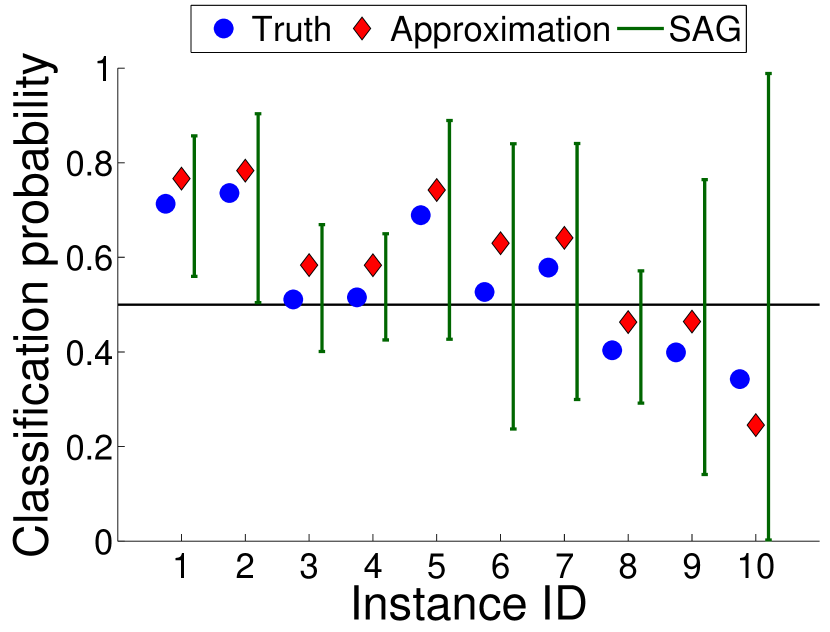
We first investigated several properties of the SAG method for the logistic regression (2) by applying it to four benchmark datasets summarized in Table 1.

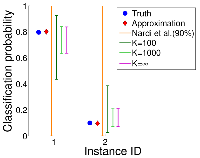
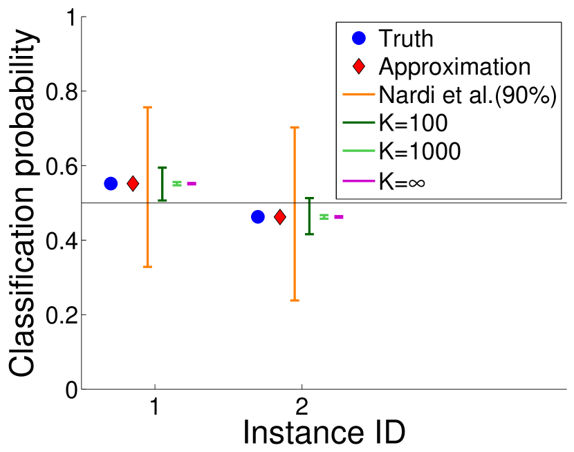
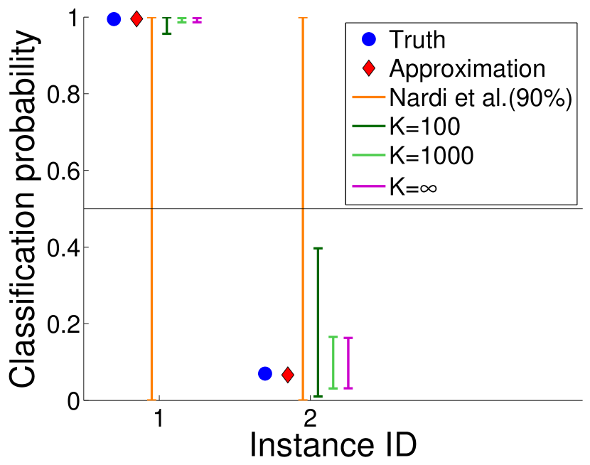
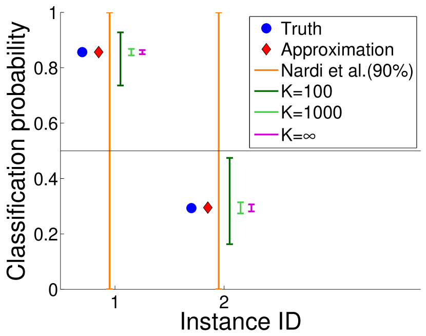
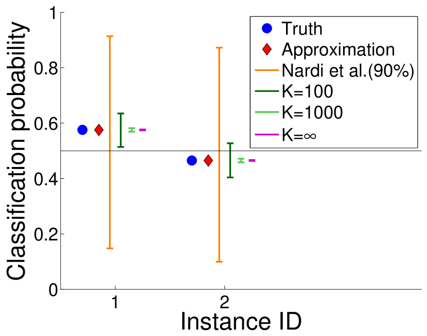
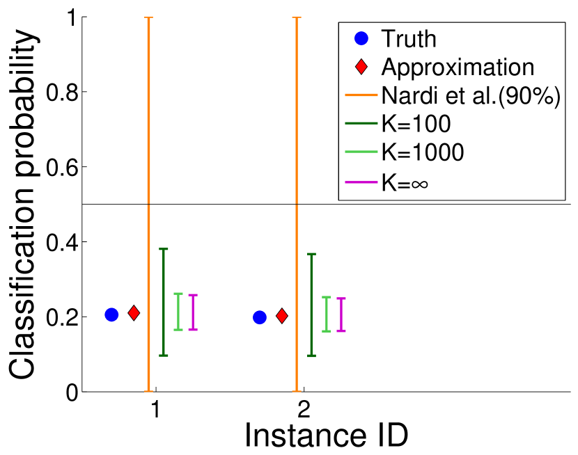
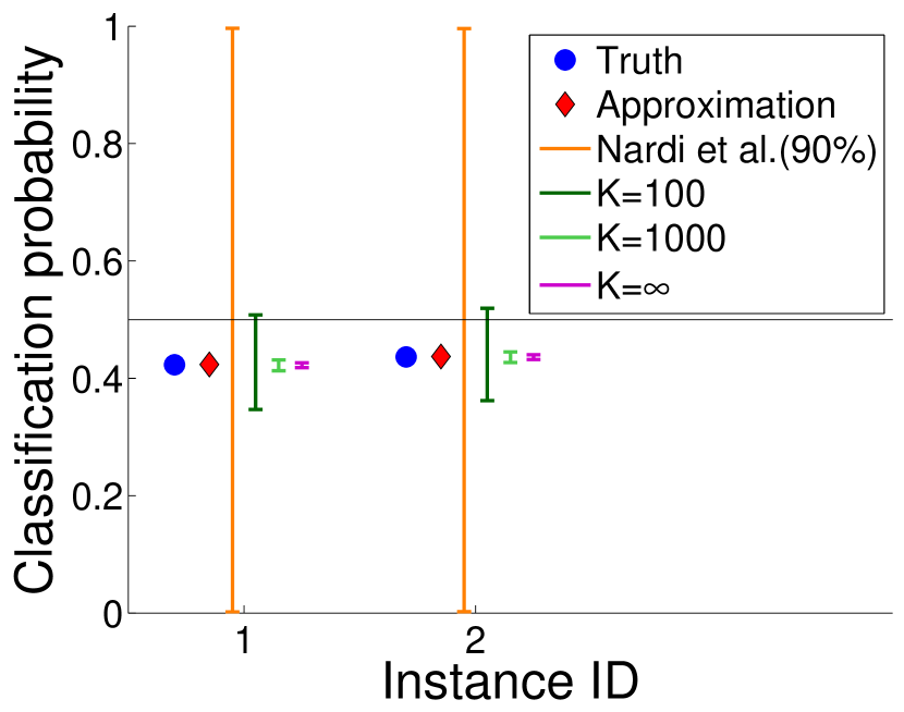
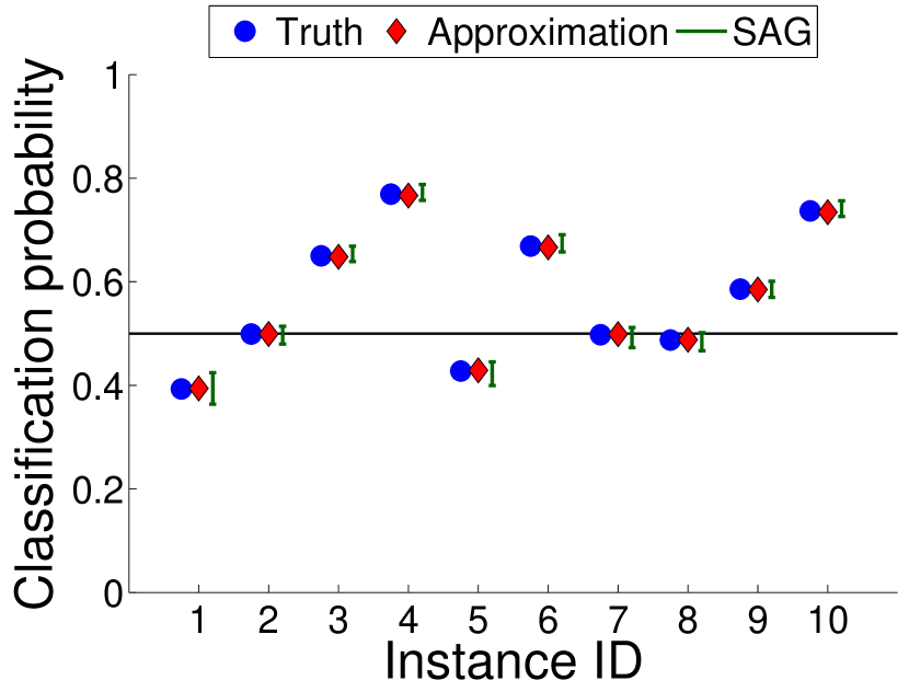
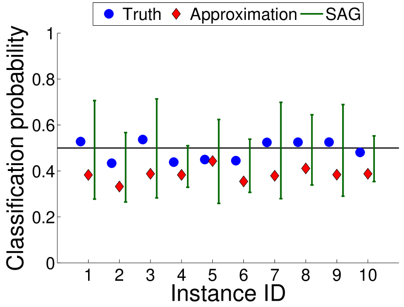
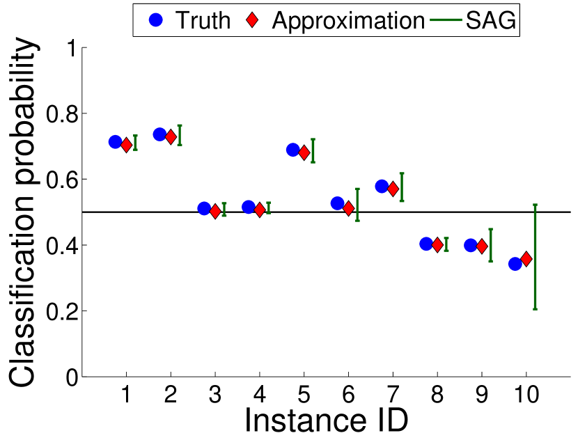
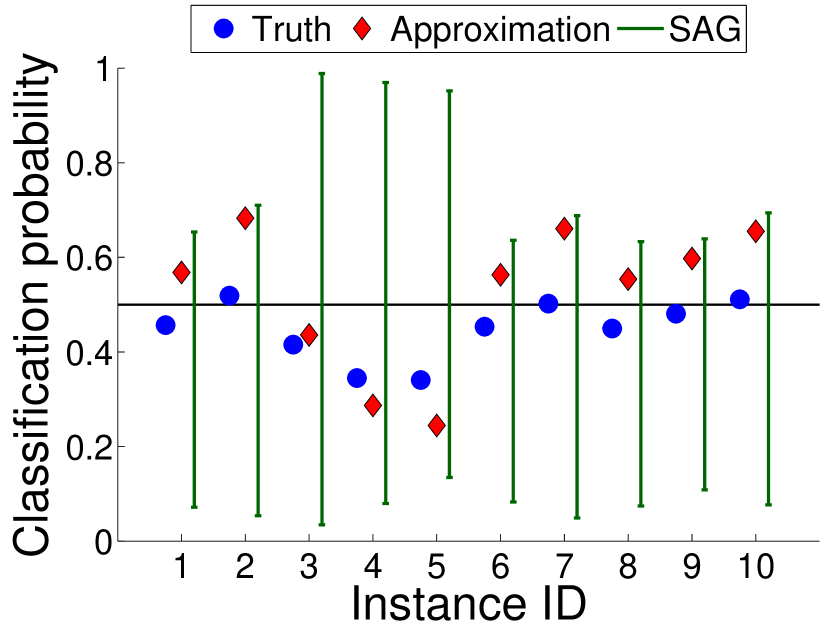
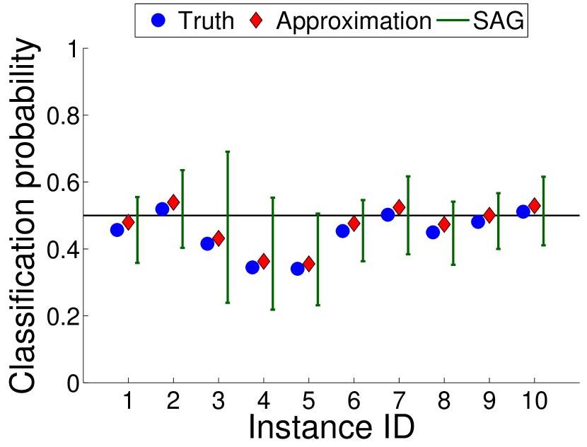
First, in Figure 3, we compared the tightness of the bounds on the predicted classification probabilities for two randomly chosen validation instances $\bm{x}_{i}$ defined as $p(\bm{x}_{i}):=1/(1+\exp(-\bm{x}_{i}^{\top}\bm{w}^{*}))$, $i=1,2$. In the figure, four types of intervals are plotted. The orange ones are Nardi et al.’s probabilistic bounds [5] with the probability 90% (see (5)). The blue, green and purple ones were obtained by the SAG method with $K=100,1000\text{ and }\infty$, respectively, where $K$ is the number of pieces in the piecewise-linear approximations. Here, $K=\infty$ means that the true loss function $\ell$ was used as the two surrogate loss functions $\phi$ and $\psi$. The results clearly indicate that bounds obtained by the SAG method are clearly tighter than those by Nardi et al.’s approach despite that the latter is probabilistic and cannot be securely computed in practice. When comparing the results with different $K$, we can confirm that large $K$ yields tighter bounds. The results with $K=1000$ are almost as tight as those obtained with the true loss function ($K=\infty$).

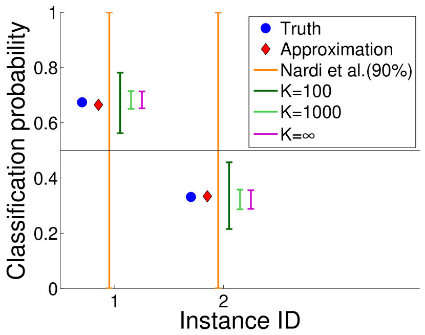
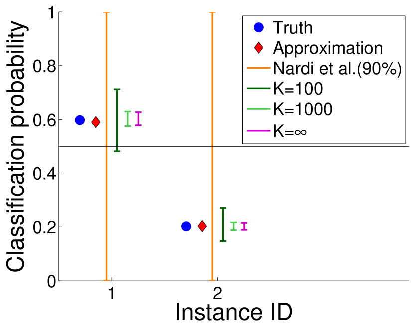
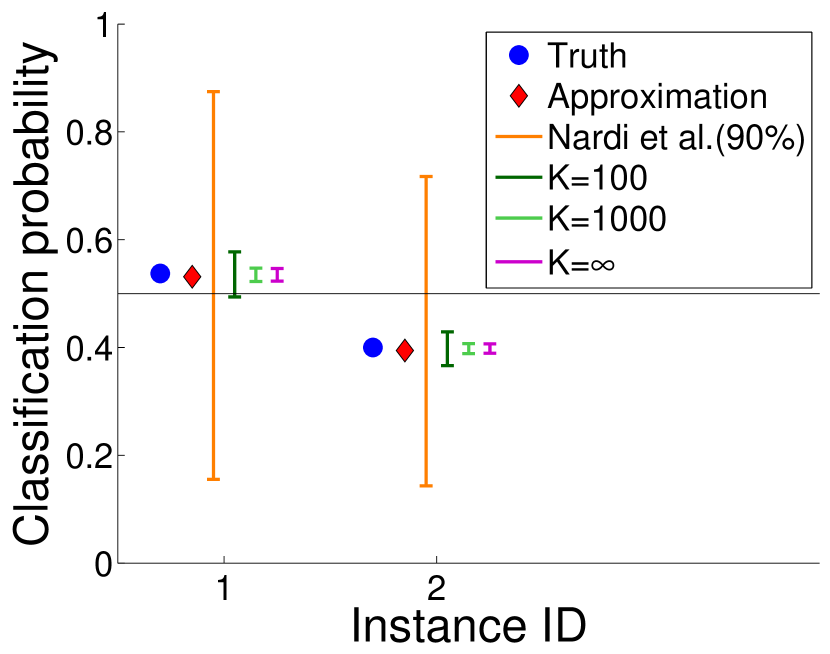
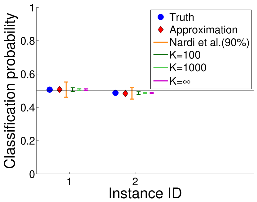
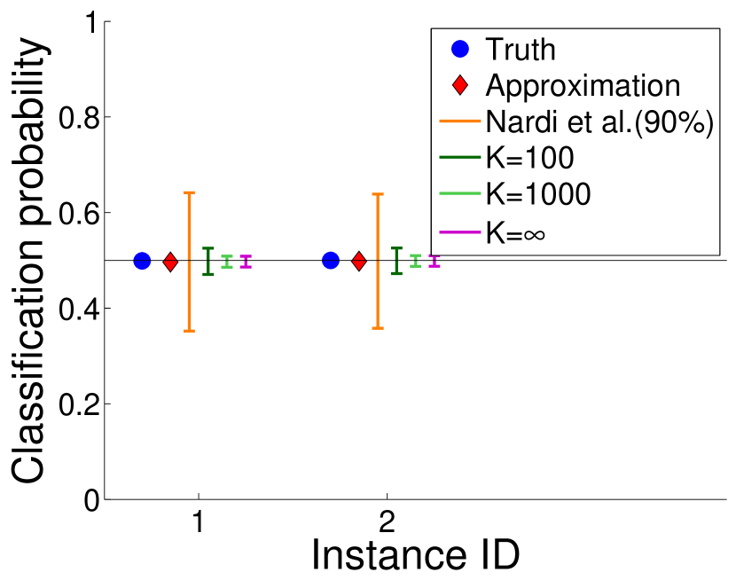
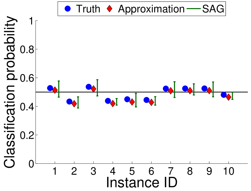
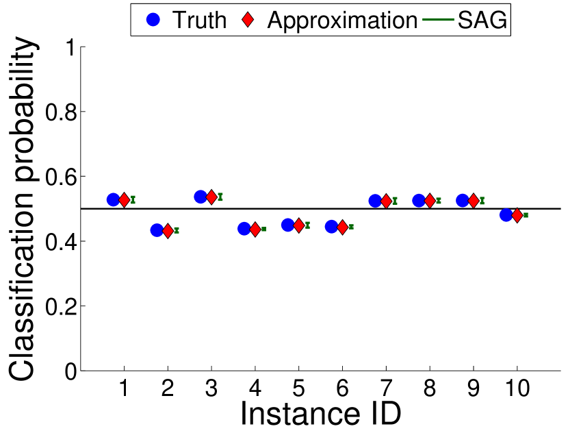
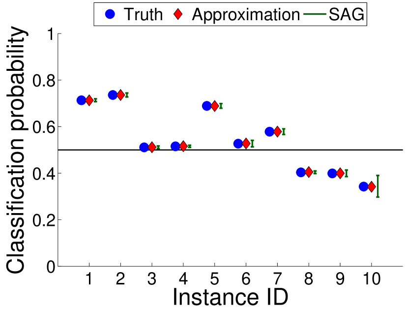
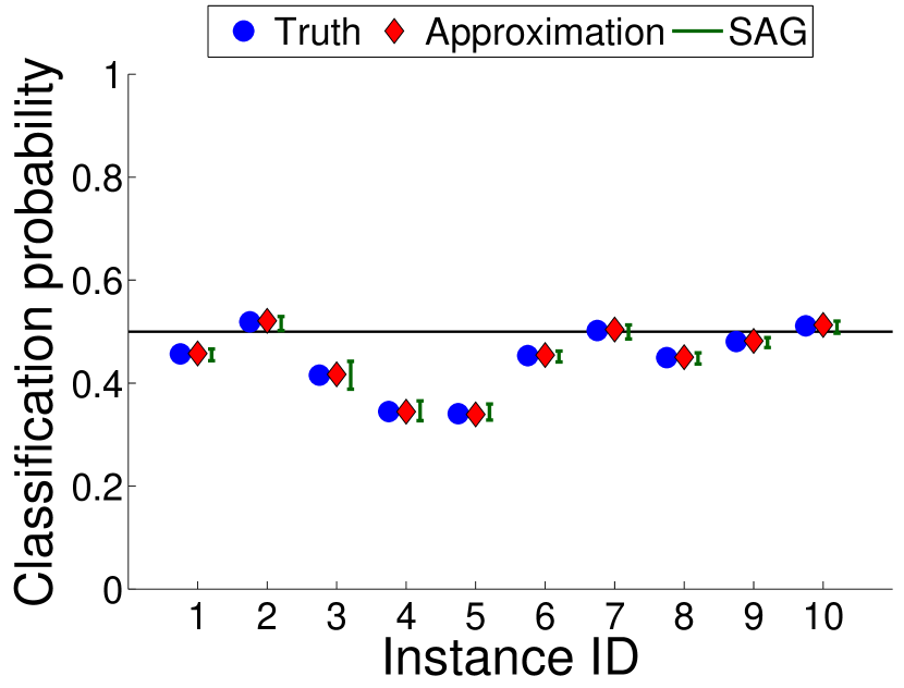
Figure 4 also shows similar plots. Here, we investigated how the tightness of the SAG bounds changes with the quality of the approximate solution $\hat{\bm{w}}$. In order to consider approximate solutions with different levels of quality, we computed three approximate solutions with $L=10,100\text{ and }1000$ in Nardi et al.’s approach, where $L$ is the sample size used for approximating the logistic function (see §2.3). The results clearly indicate that tighter bounds are obtained when the quality of the approximate solution is higher (i.e., larger $L$).

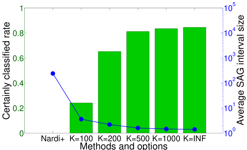
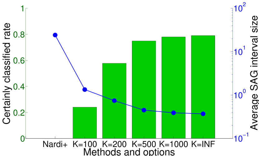
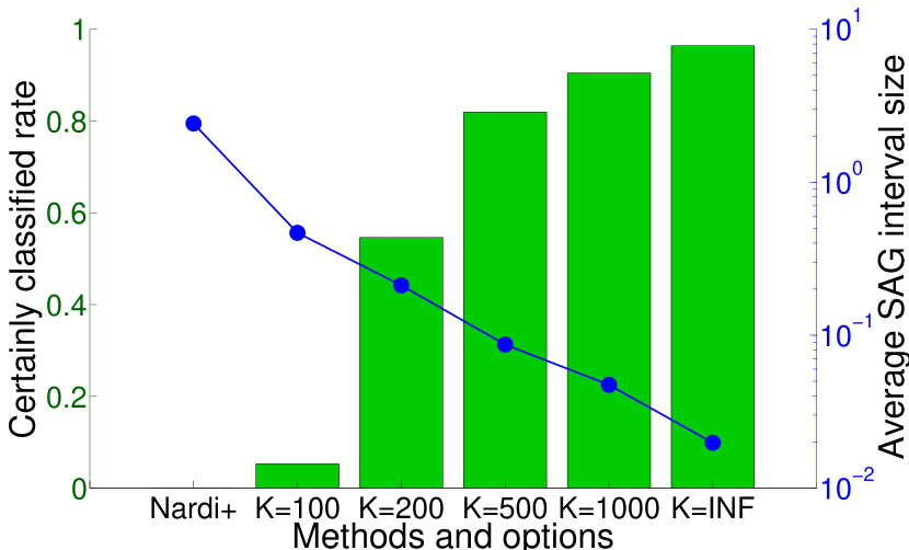
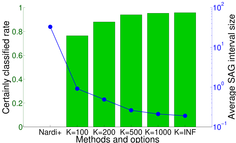
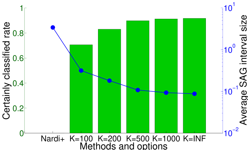
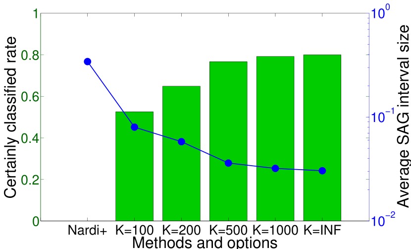
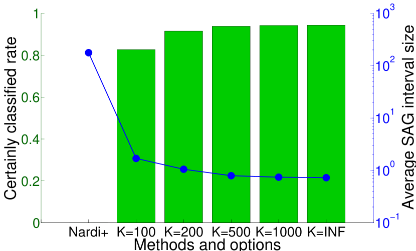
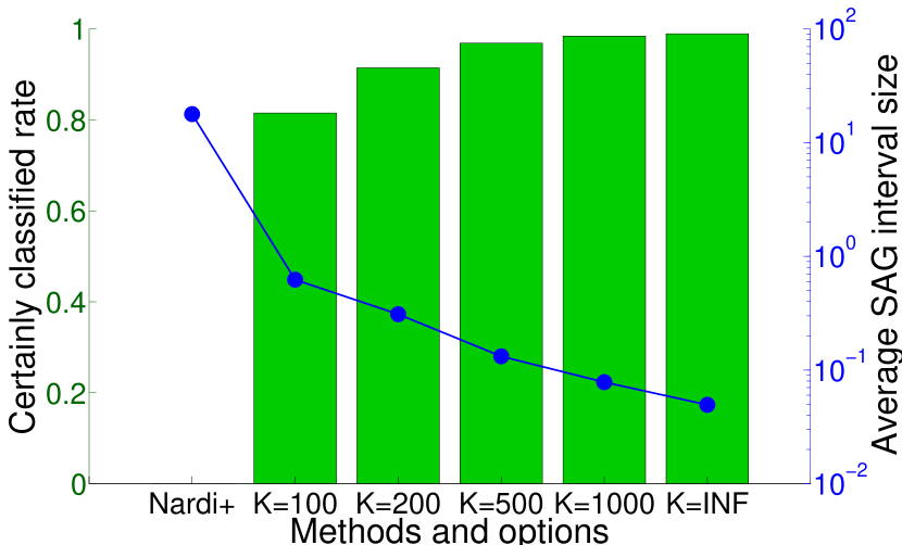
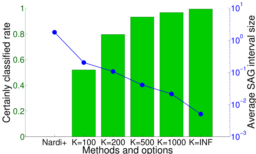
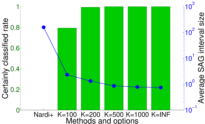
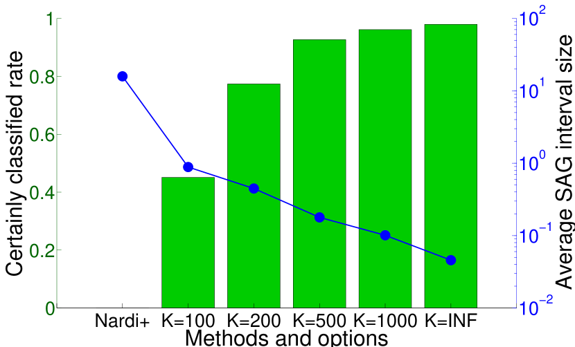
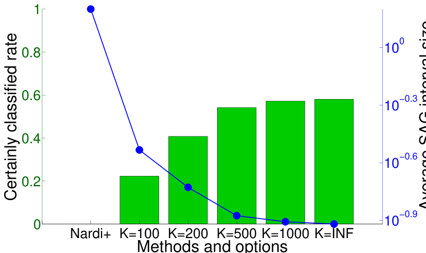
Figure 5 illustrates how the SAG bounds can be useful in binary classification problems. In binary classification problems, if a lower bound of the classification probability is greater than 0.5, the instance would be classified to positive class. Similarly, if an upper bound of the classification probability is smaller than 0.5, the instance would be classified to negative class. The green histograms in the figure indicate how many percent of the validation instances can be certainly classified as positive or negative class based on the SAG bounds. The blue lines indicate the average length of the SAG intervals, i.e., the difference between the upper and the lower bounds. The results clearly indicate that, as the number of pieces $K$ increases in the SAG method, the tighter bounds are obtained, and more validation instances can be certainly classified. On the other hand, probabilistic bounds in Nardi et al.’s approach cannot provide certain classification results because their bounds are too loose.

Table 2: Computation Time for obtaining bounds per instance

$K$	100	200	500	1000
Time(s)	381.089	790.674	1877.176	3717.569

Finally, we examined the computation time for computing the SAG bounds. Table 2 shows the computation time per instance with $K=\{100,200,500,1000\}$. The results suggest that the computational cost is almost linear in $K$, meaning that the computation of piecewise-linear functions dominates the cost. Although this task can be completely parallelized per instance, further speed-up would be desired when $K$ is larger than 1000.

5.2 Poisson and exponential regressions

(A) Poisson regression

(B) Exponential regression

Figure 6: Proposed bounds for Poisson and exponential regressions

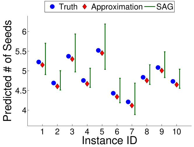
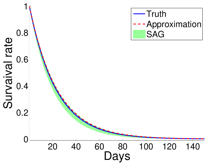
We applied the SAG method to Poisson regression (3) and exponential regression (4). Poisson regression was applied to a problem for predicting the number of produced seeds . Exponential regression was applied to a problem for predicting survival time of lung cancer patients . The results are shown in Figure 6. The left plot (A) shows the result of Poisson regression, where the SAG intervals on the predicted number of seeds are plotted for several randomly chosen instances. The right plot (B) shows the SAG bounds on the predicted survival probability curve, in which we can confirm that the true survival probability curve is included in the SAG bound.

5.3 Privacy-preserving logistic regression to genomic and clinical data analysis

Figure 7: Bounds of coefficients for disease risk evaluation

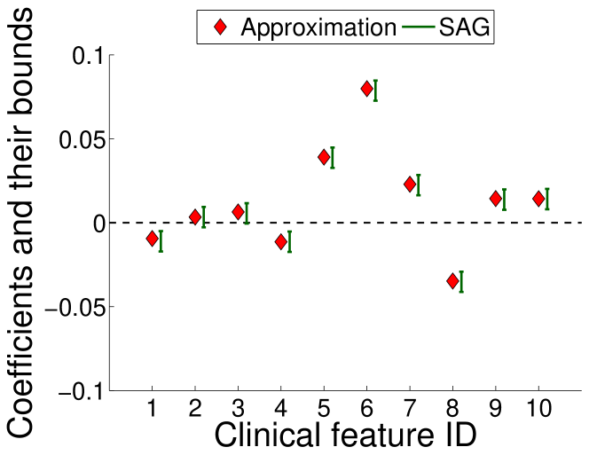
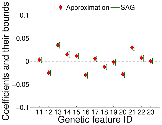
Finally, we apply the SAG method to a logistic regression on a genomic and clinical data analysis, which is the main motivation of this work (§1). In this problem, we are interested in modeling the risk of a disease based on genomic and clinical information of potential patients. The difficulty of this problem is that genomic information were collected in a research institute, while clinical information were collected in a hospital, and both institutes do not want to share their data to others. However, since the risk of the disease is dependent both on genomic and clinical features, it is quite valuable to use both types of information for the risk modeling. Our goal is to find genomic and clinical features that highly affect the risk of the disease. To this end, we use the SAG method for computing the bounds of coefficients of the logistic regression model as described in §3.

In this experiment, 13 genomic (SNP) and 10 clinical features of 134 potential patients are provided from a research institute and a hospital, respectively . The SAG bounds on each of these 23 coefficients are plotted in Figure 7. Although we do not know the true coefficient values, we can at least identify features that positively/negatively correlated with the disease risk (note that, if the lower/upper bound is greater/smaller than 0, the feature is guaranteed to have positive/negative coefficient in the logistic regression model).

6 Conclusions

We studied empirical risk minimization (ERM) problems under secure multi-party computation (MPC) frameworks. We developed a novel technique called secure approximation guarantee (SAG) method that can be used when only an approximate solution is available due to the difficulty of secure non-linear function evaluations. The key property of the SAG method is that it can securely provide the bounds on the true solution, which is practically valuable as we illustrated in benchmark data experiments and in our motivating problem on genomic and clinical data.

Appendix

Proofs of Theorem 1 and Corollary 2 (bounds of $\bm{w}^{*}$ from ${\hat{\bm{w}}}$)

First we present the following proposition which will be used for proving Theorem 1.

Proposition 6.

Consider the following general problem:

$$\min_{z}~{}g(z)~{}~{}~{}{\rm s.t.}~{}z\in{\cal Z},$$ (11)

where $g:{\cal Z}\to\mathbb{R}$ is a subdifferentiable convex function and ${\cal Z}$ is a convex set. Then a solution $z^{*}$ is the optimal solution of (11) if and only if

$$\nabla g(z^{*})^{\top}(z^{*}-z)\leq 0~{}~{}~{}\forall~{}z\in{\cal Z},$$

where $\nabla g(z^{*})$ is the subgradient vector of $g$ at $z=z^{*}$.

See, for example, Proposition B.24 in [22] for the proof of Proposition 6.

Proof of Theorem 1.

Using a slack variable $\xi\in\mathbb{R}$, let us first rewrite the minimization problem (1) as

$$\min_{\bm{w}\in\mathbb{R}^{d},\xi\in\mathbb{R}}J(\bm{w},\xi):=\xi+\frac{\lambda}{2}\|\bm{w}\|^{2}\text{\quad s.t.\quad}\xi\geq\frac{1}{n}\sum_{i\in[n]}\ell(y_{i},\bm{x}_{i}^{\top}\bm{w}).$$ (12)

Note that the optimal solution of the problem (12) is $\bm{w}=\bm{w}^{*}$ and $\xi=\xi^{*}:=\frac{1}{n}\sum_{i\in[n]}\ell(y_{i},\bm{x}_{i}^{\top}\bm{w}^{*})$. Using the definitions of $\psi$ and $\Psi$, we have $\frac{1}{n}\sum_{i\in[n]}\ell(y_{i},\bm{x}_{i}^{\top}\hat{\bm{w}})\leq\frac{1}{n}\sum_{i\in[n]}\psi(y_{i},\bm{x}_{i}^{\top}\hat{\bm{w}})=\Psi(\hat{\bm{w}})$. It means that $(\hat{\bm{w}},\Psi(\hat{\bm{w}}))$ is a feasible solution of the problem (12). Applying this fact into Proposition 6, we have

$$\nabla J(\bm{w}^{*},\xi^{*})^{\top}\left(\left[\begin{array}[]{c}\bm{w}^{*}\\ \xi^{*}\end{array}\right]-\left[\begin{array}[]{c}\hat{\bm{w}}\\ \Psi(\hat{\bm{w}})\end{array}\right]\right)\leq 0,$$ (17)

where $\nabla J(\bm{w}^{*},\xi^{*})\in\mathbb{R}^{d+1}$ is the gradient of the objective function in (12) evaluated at $(\bm{w}^{*},\xi^{*})$. Since $J(\bm{w},\xi)$ is a quadratic function of $\bm{w}$ and $\xi$, we can write $\nabla J(\bm{w}^{*},\xi^{*})$ explicitly, and (17) is written as

$$\lambda\|\bm{w}^{2}\|+\xi^{*}-\lambda\bm{w}^{*\top}\hat{\bm{w}}-\Psi(\hat{\bm{w}})\leq 0$$

$$\Leftrightarrow~{} \lambda\|\bm{w}^{*2}\|+\frac{1}{n}\sum_{i\in[n]}\ell(y_{i},\bm{x}_{i}^{\top}\bm{w}^{*})-\lambda\bm{w}^{*\top}\hat{\bm{w}}-\Psi(\hat{\bm{w}})\leq 0$$ (18)

From the definition of $\phi$ and $\Phi$, we have

$$\frac{1}{n}\sum_{i\in[n]}\ell(y_{i},\bm{x}_{i}^{\top}\bm{w}^{*})\geq\frac{1}{n}\sum_{i\in[n]}\phi(y_{i},\bm{x}_{i}^{\top}\bm{w}^{*})=\Phi(\bm{w}^{*}).$$

Plugging this into (18), we have

$$\lambda\|\bm{w}^{*2}\|+\Phi(\bm{w}^{*})-\lambda\bm{w}^{*\top}\hat{\bm{w}}-\Psi(\hat{\bm{w}})\leq 0$$ (19)

Furthermore, noting that $\phi$ and $\Phi$ are convex with respect to $\bm{w}$, by the definition of convex functions we get

$$\Phi(\bm{w}^{*})\geq\Phi(\hat{\bm{w}})+\nabla\Phi(\hat{\bm{w}})^{\top}(\bm{w}^{*}-\hat{\bm{w}}).$$ (20)

By plugging (20) into (19),

$$\lambda\|\bm{w}^{*2}\|+\Phi(\hat{\bm{w}})+\nabla\Phi(\hat{\bm{w}})^{\top}(\bm{w}^{*}-\hat{\bm{w}})-\lambda\bm{w}^{*\top}\hat{\bm{w}}-\Psi(\hat{\bm{w}})\leq 0$$ (21)

Noting that (21) is a quadratic function of $\bm{w}^{*}$, we obtain

$$\left\|\bm{w}^{*}-\frac{1}{2}\left(\hat{\bm{w}}-\frac{1}{\lambda}\nabla\Phi(\hat{\bm{w}})\right)\right\|^{2}\leq\left\|\frac{1}{2}\left(\hat{\bm{w}}+\frac{1}{\lambda}\nabla\Phi(\hat{\bm{w}})\right)\right\|^{2}+\frac{1}{\lambda}\left(\Psi(\hat{\bm{w}})-\Phi(\hat{\bm{w}})\right).$$

It means that the optimal solution $\bm{w}^{*}$ is within a ball with the center $\bm{m}(\hat{\bm{w}})$ and the radius $r(\hat{\bm{w}})$, which completes the proof. ∎

Next, we prove Corollary 2.

Proof of Corollary 2.

We show that the lower bound of the linear model output value $\bm{w}^{*\top}\bm{x}$ is $\bm{x}^{\top}\bm{m}(\hat{\bm{w}})-\|\bm{x}\|r(\hat{\bm{w}})$ under the constraint that

$$\|\bm{w}^{*}-\bm{m}(\hat{\bm{w}})\|\leq r(\hat{\bm{w}}).$$

To formulate this, let us consider the following constrained optimization problem

$$\min_{\bm{w}\in\mathbb{R}^{d}}~{}\bm{w}^{\top}\bm{x}~{}~{}~{}\text{s.t.}~{}~{}~{}\|\bm{w}-\bm{m}(\hat{\bm{w}})\|^{2}\leq r(\hat{\bm{w}})^{2}.$$ (22)

Using a Lagrange multiplier $\mu>0$, the problem (22) is rewritten as

$$\min_{\bm{w}\in\mathbb{R}^{d}}~{}\bm{w}^{\top}\bm{x}~{}~{}~{}\text{s.t.}~{}~{}~{}\|\bm{w}-\bm{m}(\hat{\bm{w}})\|^{2}\leq r(\hat{\bm{w}})^{2},$$

$$= \min_{\bm{w}\in\mathbb{R}^{d}}\max_{\mu>0}\big{(}\bm{w}^{\top}\bm{x}+\mu(\|\bm{w}-\bm{m}(\hat{\bm{w}})\|^{2}-r(\hat{\bm{w}})^{2})\big{)}$$

$$= \max_{\mu>0}\big{(}-\mu r(\hat{\bm{w}})^{2}+\min_{\bm{w}}\big{(}\mu\|\bm{w}-\bm{m}(\hat{\bm{w}})\|^{2}+\bm{w}^{\top}\bm{x}\big{)}\big{)}$$

$$= \max_{\mu>0}~{}H(\mu):=\big{(}-\mu r(\hat{\bm{w}})^{2}-\frac{\|\bm{x}\|^{2}}{4\mu}+\bm{x}^{\top}\bm{m}(\hat{\bm{w}})\big{)},$$

where $\mu$ is strictly positive because the constraint $\|\bm{w}-\bm{m}(\hat{\bm{w}})\|^{2}\leq r(\hat{\bm{w}})^{2}$ is strictly active at the optimal solution. By letting $\partial H(\mu)/\partial\mu=0$, the optimal $\mu$ is written as

$$\mu^{*}:=\frac{\|\bm{x}\|}{2r(\hat{\bm{w}})}=\arg\max_{\mu>0}~{}H(\mu).$$

Substituting $\mu^{*}$ into $H(\mu)$,

$$\bm{x}^{\top}\bm{m}(\hat{\bm{w}})-\|\bm{x}\|r(\hat{\bm{w}})=\max_{\mu>0}~{}H(\mu).$$

The upper bound part can be shown similarly. ∎

Proof of Theorem 3 (Protocol evaluating piecewise linear function and its subderivative securely)

First we explain the outline of the protocol of secure comparison by Veugen et al. [20]. The protocol returns the result of comparison $E_{pk_{B}}(I_{q>0})$ (given to party A) for the encrypted values $E_{pk_{B}}(q)$ (owned by party A) with the following two steps:

• Party A and B obtain $q_{A}:=R$ and $q_{B}:=q+R$, respectively, where $R$ is a random value, and

• Party A and B compare $q_{A}$ and $q_{B}$ with the implementation of bit-wise comparison with Paillier cryptosystem (see the original paper).

Let us denote the protocol of the latter by $SC(q_{A},q_{B})\rightarrow(E_{pk_{B}}(I_{q_{A}>q_{B}}),E_{pk_{A}}(I_{q_{A}>q_{B}}))$, that is, $SC$ is a protocol comparing two private, unencrypted values owned by two parties $q_{A}$, $q_{B}$.

The protocol for Theorem 3 is as follows:

1. Party A computes $E_{pk_{B}}(s)=E_{pk_{B}}(s_{A}+s_{B})$ from $E_{pk_{B}}(s_{A})$ and $E_{pk_{A}}(s_{B})$ as follows:

   • Party B generates a random value $R\in\mathbb{Z}_{N/2}$ ($N$ is defined in §2.2), then sends $E_{pk_{A}}(s_{B}-R)=E_{pk_{A}}(s_{B})^{-R}$ and $E_{pk_{B}}(R)$ to party A.

   • Party A decrypts $E_{pk_{A}}(s_{B}-R)$ and computes $E_{pk_{B}}(s_{A}+s_{B})$ as: $E_{pk_{B}}(s_{A}+s_{B})=E_{pk_{B}}(s_{A}+s_{B}-R+R)=E_{pk_{B}}(s_{A}+s_{B}-R)E_{pk_{B}}(R)=E_{pk_{B}}(s_{A})^{s_{B}-R}E_{pk_{B}}(R)$.

   See [23] for the security of the part.

2. With the similar protocol to Veugen et al.’s, party A and B obtains $p_{A}$ and $p_{B}$, respectively, where $p_{A}$ and $p_{B}$ are randomized and satisfy $p_{A}+p_{B}=s$.

3. Compute $t_{j}=I_{p_{A}+p_{B}>T_{j}}$ securely with $SC$:

   $$SC(p_{A},T_{j}-p_{B})\rightarrow(E_{pk_{B}}(t_{j}),E_{pk_{A}}(t_{j})),$$ (23)

4. Party A computes $E_{pk_{B}}(o_{j})$ from $E_{pk_{B}}(t_{j})$:

   $$E_{pk_{B}}(o_{j})=E_{pk_{B}}(t_{j-1}-t_{j})=E_{pk_{B}}(t_{j-1})\cdot E_{pk_{B}}(t_{j})^{-1}$$

   Party B similarly computes for $E_{pk_{A}}$. The idea is shown in Figure 8.

5. Party A computes $g_{Aj}:=\alpha_{j}p_{A}+\beta_{j}$, and party B $g_{Bj}:=\alpha_{j}p_{B}$ for all $j\in[K]$. Note that $g_{Aj}+g_{Bj}=\alpha_{j}s+\beta_{j}$.

6. Compute encrypted $g_{A}$ and $g_{B}$. Because $g_{A}+g_{B}=g(s)$ after taking $g_{A}=\sum_{j\in[K]}o_{j}g_{Aj}$ and $g_{B}=\sum_{j\in[K]}o_{j}g_{Bj}$ (see (9) in §4), party A computes $E_{pk_{B}}(g_{A})$ as

   $$E_{pk_{B}}(g_{A})=E_{pk_{B}}\left(\sum_{j\in[K]}o_{j}g_{Aj}\right)=\prod_{j\in[K]}E_{pk_{B}}(o_{j})^{g_{Aj}}.$$

   Party B similarly computes $E_{pk_{A}}(g_{B})$.

Figure 8: Computing $o_{j}$ from $t_{j}$ in the protocol $SPLC$

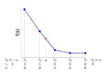
To obtain the subderivative $g^{\prime}(s)=\sum_{j\in[K]}o_{j}\alpha_{j}$, during the protocol for Theorem 3, party A computes $E_{pk_{B}}(g^{\prime}(s))$ as

$$E_{pk_{B}}(g^{\prime}(s))=E_{pk_{B}}\left(\sum_{j\in[K]}o_{j}\alpha_{j}\right)=\prod_{j\in[K]}E_{pk_{B}}(o_{j})^{\alpha_{j}}.$$

Party B similarly computes $E_{pk_{A}}(g^{\prime}(s))$.

Proof of Theorem 5 (Protocol evaluating the upper and the lower bounds)

Protocol 1 securely evaluates the upper bound $UB$ and the lower bound $LB$, where $\overline{sqrt}$ is an upper bound of the square root function implemented as a piecewise linear function. Note that taking $r$ larger does not lose the validity of the bounds (looser bounds are obtained) as

$$\tilde{\bm{x}}^{\top}\bm{m}-\overline{\|\tilde{\bm{x}}\|r}\leq\tilde{\bm{x}}^{\top}\bm{m}-\|\tilde{\bm{x}}\|r,$$

$$\tilde{\bm{x}}^{\top}\bm{m}+\overline{\|\tilde{\bm{x}}\|r}\geq\tilde{\bm{x}}^{\top}\bm{m}+\|\tilde{\bm{x}}\|r.$$

The security is proved as follows: all techniques used in the protocol are secure with the same discussions as previous. The remaining problem is that whether party A can guess $\tilde{\bm{x}}_{B}$ from $UB$ and $LB$. Party A can know $UB+LB=\bm{\tilde{x}}^{\top}\bm{m}=\bm{\tilde{x}}_{A}^{\top}\bm{m}_{A}+\bm{\tilde{x}}_{B}^{\top}\bm{m}_{B}$ and $UB-LB=\overline{\|\tilde{\bm{x}}\|r}=\overline{sqrt}((\|\tilde{\bm{x}}_{A}\|^{2}+\|\tilde{\bm{x}}_{B}\|^{2})(r_{A}^{2}+r_{B}^{2}))$. However, because party A does not know $\bm{m}_{A}$, $\bm{m}_{B}$, $r_{A}^{2}$ or $r_{B}^{2}$, party A cannot guess $\tilde{\bm{x}}_{B}$ either.

Protocol 1 Protocol for bound computation

public

$\overline{sqrt}$

Input of A

$E_{pk_{B}}(\bm{m}_{A}),E_{pk_{B}}(r_{A}^{2}),\tilde{\bm{x}}_{A}$

Input of B

$E_{pk_{B}}(\bm{m}_{B}),E_{pk_{B}}(r_{B}^{2}),\tilde{\bm{x}}_{B}$

Output of A

$UB,LB$

Output of B

$\emptyset$

1. Party A and B computes:

   party A:$E_{pk_{B}}(\tilde{\bm{x}}_{A}^{\top}\bm{m}_{A}),E_{pk_{A}}(\|\tilde{\bm{x}}_{A}\|^{2})$

   party B:$E_{pk_{A}}(\tilde{\bm{x}}_{A}^{\top}\bm{m}_{B}),\|\tilde{\bm{x}}_{B}\|^{2}$

2. Party A sends $E_{pk_{B}}(\tilde{\bm{x}}_{A}^{\top}\bm{m}_{A}),E_{pk_{A}}(\|\tilde{\bm{x}}_{A}\|^{2}),E_{pk_{B}}(r_{A}^{2})$ to B.
   Party B obtains $E_{pk_{A}}(\tilde{\bm{x}}^{\top}\bm{m}),E_{pk_{A}}(\|\tilde{\bm{x}}\|^{2}),E_{pk_{A}}(r^{2})$.
   // The similar manner to the protocol for Theorem 3, step 1

3. Compute $E_{pk_{B}}(\|\tilde{\bm{x}}\|^{2}r^{2})$ using the protocol for multiplication in [21].

4. Compute $\overline{\|\tilde{\bm{x}}\|r}$ with $SPL$:
   $SPL(E_{pk_{B}}(0),E_{pk_{B}}(\|\tilde{\bm{x}}\|^{2}r^{2}))\to(q_{A},q_{B})$ //$q_{A}+q_{B}=\overline{\|\tilde{\bm{x}}\|r}$

5. Party A sends $E_{pk_{B}}(q_{B})$ to B.
   Party B obtains $q_{B}$ and thus $E_{pk_{A}}(\overline{\|\tilde{\bm{x}}\|r})=E_{pk_{A}}(q_{A})^{q_{B}}$.
   Party B computes the followings and sends to A.
   $E_{pk_{A}}(UB)\leftarrow E_{pk_{A}}(\tilde{\bm{x}}^{\top}\bm{m}+\overline{\|\tilde{\bm{x}}\|r})$
   $E_{pk_{A}}(LB)\leftarrow E_{pk_{A}}(\tilde{\bm{x}}^{\top}\bm{m}-\overline{\|\tilde{\bm{x}}\|r})$

6. Party A obtains $UB,LB$ by decrypting them.

Example Protocol for the Logistic Regression

We show the detailed implementation of secure ball computation ($SBC$, Theorem 4) in §4 for the logistic regression, including how to use the secure computation of piecewise linear functions ($SPL$, Theorem 3).

For the logistic regression (§2.1), ${\cal Y}=\{-1,+1\}$, and we take $u(s)=\log(1+\exp(-s))$, $s=\bm{x}^{\top}\bm{w}$ and $v(y,\bm{x}^{\top}\bm{w})=-y\bm{x}^{\top}\bm{w}$ in Theorem 4.

To apply this for $SPL$, we set $E_{pk_{B}}(s_{A}):=E_{pk_{B}}(\bm{x}_{A}^{\top}{\hat{\bm{w}}}_{A})$ and $E_{pk_{A}}(s_{B}):=E_{pk_{A}}(\bm{x}_{B}^{\top}{\hat{\bm{w}}}_{B})$ since we assume party A and B knows $E_{pk_{B}}({\hat{\bm{w}}}_{A})$ and $E_{pk_{A}}({\hat{\bm{w}}}_{B})$, respectively. Note that $s_{A}+s_{B}=s$ because $\bm{x}=[\bm{x}_{A}^{\top}~{}\bm{x}_{B}^{\top}]^{\top}$ and $\bm{w}=[\bm{w}_{A}^{\top}~{}\bm{w}_{B}^{\top}]^{\top}$. Take piecewise linear functions $\underline{u}(s)$ and $\overline{u}(s)$ as lower and upper bounds of $u(s)$, respectively. With it, we can compute $\phi$, $\psi$ and $\nabla\phi$ in $SAG$ as follows:

$$\psi|_{\bm{w}={\hat{\bm{w}}}}- \phi|_{\bm{w}={\hat{\bm{w}}}}=\overline{u}(\bm{x}^{\top}{\hat{\bm{w}}})-\underline{u}(\bm{x}^{\top}{\hat{\bm{w}}}),$$

$$\nabla\phi|_{\bm{w}={\hat{\bm{w}}}} =\underline{u}^{\prime}(\bm{x}^{\top}{\hat{\bm{w}}})\left.\frac{\partial s}{\partial\bm{w}}\right|_{\bm{w}={\hat{\bm{w}}}}+\left.\frac{\partial v}{\partial\bm{w}}\right|_{\bm{w}={\hat{\bm{w}}}}$$

$$=\underline{u}^{\prime}(\bm{x}^{\top}{\hat{\bm{w}}})\left.\frac{\partial}{\partial\bm{w}}\bm{x}^{\top}\bm{w}\right|_{\bm{w}={\hat{\bm{w}}}}+\left.\frac{\partial}{\partial\bm{w}}y\bm{x}^{\top}\bm{w}\right|_{\bm{w}={\hat{\bm{w}}}}$$

$$=(\underline{u}^{\prime}(\bm{x}^{\top}{\hat{\bm{w}}})+y)\bm{x},$$

which are all computable with $SPL$.

After these preparations, we can conduct the protocol $SBC$ as Protocol 2.

Protocol 2 Secure Ball Computation protocol (SBC)

Public

$\phi:=\underline{u}(s)-y\bm{x}^{\top}\bm{w}$, $\psi:=\overline{u}(s)-y\bm{x}^{\top}\bm{w}$

Input from A

$\{\bm{x}_{iA}\}_{i\in[n]},E_{pk_{B}}({\hat{\bm{w}}}_{A})$

Input from B

$\{\bm{x}_{iB},y_{i}\}_{i\in[n]},E_{pk_{A}}({\hat{\bm{w}}}_{B})$

Output to A

$E_{pk_{B}}(\bm{m}_{A}),E_{pk_{B}}(r_{A}^{2})$

Output to B

$E_{pk_{A}}(\bm{m}_{B}),E_{pk_{A}}(r_{B}^{2})$ (where $r_{A}^{2}+r_{B}^{2}=r^{2}$)

1. Party B sends $E_{pk_{B}}(\bm{y})$ to party A.

2. Party A and B compute encrypted $\Phi$, $\Psi$ and $\nabla\Phi$ at $\bm{w}={\hat{\bm{w}}}$.

3. Party A does:

   1. for $i=1$ to $n$:
       $SPLC(E_{pk_{B}}(\bm{x}_{iA}^{\top}{\hat{\bm{w}}}_{A}),E_{pk_{A}}(\bm{x}_{iB}^{\top}{\hat{\bm{w}}}_{B}))\rightarrow\left(E_{pk_{B}}(\underline{u}^{*}_{iA}),E_{pk_{A}}(\underline{u}^{*}_{iB})\right)$,
       $SPLC(E_{pk_{B}}(\bm{x}_{iA}^{\top}{\hat{\bm{w}}}_{A}),E_{pk_{A}}(\bm{x}_{iB}^{\top}{\hat{\bm{w}}}_{B}))\rightarrow\left(E_{pk_{B}}(\overline{u}^{*}_{iA}),E_{pk_{A}}(\overline{u}^{*}_{iB})\right)$

   2. // Note: $E(a)^{1/n}$ is in reality computed as $E(a)^{M/n}$,
      //  where $M$ is the magnification constant.
      // Note: $E(a)^{\bm{\eta}}$ ($\bm{\eta}$: a vector) means $[E(a)^{\eta_{1}}~{}E(a)^{\eta_{2}}~{}\cdots]^{\top}$.

   3. $E_{pk_{B}}(\Psi_{A}-\Phi_{A})$
      $\leftarrow E_{pk_{B}}\left(\frac{1}{n}\sum_{i\in[n]}[\overline{u}^{*}_{iA}-y_{i}\bm{x}_{iA}^{\top}{\hat{\bm{w}}}_{A}]-\frac{1}{n}\sum_{i\in[n]}[\underline{u}^{*}_{iA}-y_{i}\bm{x}_{iA}^{\top}{\hat{\bm{w}}}_{A}]\right)$
      $=E_{pk_{B}}\left(\frac{1}{n}\sum_{i\in[n]}[\overline{u}^{*}_{iA}-\underline{u}^{*}_{iA}]\right)$
      $=\left[\prod_{i\in[n]}E_{pk_{B}}\left(\overline{u}^{*}_{iA}\right)\right]^{1/n}\left[\prod_{i\in[n]}E_{pk_{B}}\left(\underline{u}^{*}_{iA}\right)\right]^{-1/n}$
      // $\Phi_{A}+\Phi_{B}=\Psi$, $\Psi_{A}+\Psi_{B}=\Psi$

   4. $E_{pk_{B}}(\nabla\Phi_{A})\leftarrow E_{pk_{B}}\left(\frac{1}{n}\sum_{i\in[n]}[\underline{u}^{\prime}(\bm{x}_{i}^{\top}\bm{w})-y_{i}]\bm{x}_{iA}\right)$
       $=\left[\prod_{i\in[n]}E_{pk_{B}}(\underline{u}^{\prime}(\bm{x}_{i}^{\top}\bm{w}))E_{pk_{B}}(y_{i})^{-1}\right]^{(1/n)\bm{x}_{iA}}$
      // $[\nabla\Phi_{A}^{\top},\nabla\Phi_{B}^{\top}]^{\top}=\nabla\Phi$

   5. // Note: $\underline{\alpha}_{j}$ and $\underline{o}_{j}$ means $\alpha_{j}$ and $o_{j}$ for $\underline{u}$
      //  (see the subderivative computation in Theorem 3).

4. Party B does the similar.

5. Party A and B compute encrypted $\bm{m}$ and $r$.

6. Party A does:

   1. $E_{pk_{B}}(\bm{m}_{A})\leftarrow E_{pk_{B}}({\hat{\bm{w}}}_{A}-\frac{1}{\lambda}\nabla\Phi_{A})^{1/2}$

   2. Compute $E_{pk_{B}}(\|\frac{1}{2}({\hat{\bm{w}}}_{A}+\frac{1}{\lambda}\nabla\Phi_{A})\|^{2})$ from $E_{pk_{B}}(\frac{1}{2}({\hat{\bm{w}}}_{A}+\frac{1}{\lambda}\nabla\Phi_{A}))=[E_{pk_{B}}({\hat{\bm{w}}}_{A})E_{pk_{B}}(\nabla\Phi_{A})^{1/\lambda}]^{1/2}$ using the multiplication protocol in [21].

   3. $E_{pk_{B}}(r^{2}_{A})\leftarrow E_{pk_{B}}(\|\frac{1}{2}({\hat{\bm{w}}}_{A}+\frac{1}{\lambda}\nabla\Phi_{A})\|^{2})\cdot(E_{pk_{B}}(\Psi_{A})\cdot E_{pk_{B}}(\Phi_{A})^{-1})^{1/\lambda}$

7. Party B does the similar.

Remark 7.

In the description of the protocol, we omitted the maginification constant $M$ (§2.2) for simplicity. We have to notice that, summing two values magnified by $M^{a}$ and $M^{b}$, we get a value magnified by $M^{\max\{a,b\}}$. Similarly, multiplying two values magnified by $M^{a}$ and $M^{b}$, we get a value magnified by $M^{a+b}$. In the protocol, when the original data is magnified by $M$, then the final result is magnified by $M^{12}$. So we have to adjust $M$ so that $M^{12}$ times the final result does not exceed the domain of Paillier cryptosystem $\mathbb{Z}_{N}$.

References

- [1] R. Hall, S. E. Fienberg, and Y. Nardi. Secure multiple linear regression based on homomorphic encryption. Journal of Official Statistics, 27(4):669, 2011.
- [2] V. Nikolaenko, U. Weinsberg, S. Ioannidis, M. Joye, D. Boneh, and N. Taft. Privacy-preserving ridge regression on hundreds of millions of records. In 2013 IEEE Symposium on Security and Privacy (SP), pages 334–348. IEEE, 2013.
- [3] S. Laur, H. Lipmaa, and T. Mielikäinen. Cryptographically private support vector machines. In Proceedings of the 12th ACM SIGKDD international conference on Knowledge discovery and data mining (KDD2006), pages 618–624. ACM, 2006.
- [4] H. Yu, J. Vaidya, and X. Jiang. Privacy-preserving svm classification on vertically partitioned data. In Advances in Knowledge Discovery and Data Mining, pages 647–656. Springer, 2006.
- [5] Y. Nardi, S. E. Fienberg, and R. J. Hall. Achieving both valid and secure logistic regression analysis on aggregated data from different private sources. Journal of Privacy and Confidentiality, 4(1):9, 2012.
- [6] C. Dwork. Differential privacy. In 33rd International Colloquium Automata, Languages and Programming (ICALP 2006) Proceedings Part II, pages 1–12, 2006.
- [7] J. Vaidya and C. Clifton. Privacy-preserving k-means clustering over vertically partitioned data. In Proceedings of the 9th ACM SIGKDD international conference on Knowledge discovery and data mining (KDD 2003), pages 206–215. ACM, 2003.
- [8] O. Goldreich. Foundations of cryptography: volume 1, basic tools. Cambridge university press, 2001.
- [9] P. Paillier. Public-key cryptosystems based on composite degree residuosity classes. In Advances in cryptology – EUROCRYPT’99, pages 223–238. Springer, 1999.
- [10] O. Goldreich. Foundations of cryptography: volume 2, basic applications. Cambridge university press, 2004.
- [11] C. A. Yao. How to generate and exchange secrets. In The 27th Annual IEEE Symposium on Foundations of Computer Science (FOCS 1986), pages 162–167. IEEE, 1986.
- [12] L. El Ghaoui, V. Viallon, and T. Rabbani. Safe feature elimination for the lasso and sparse supervised learning problems. Pacific Journal of Optimization, 8(4):667–698, 2012.
- [13] Z. J Xiang, H. Xu, and P. J. Ramadge. Learning sparse representations of high dimensional data on large scale dictionaries. In Advances in Neural Information Processing Systems, pages 900–908, 2011.
- [14] K. Ogawa, Y. Suzuki, and I. Takeuchi. Safe screening of non-support vectors in pathwise svm computation. In Proceedings of the 30th International Conference on Machine Learning, pages 1382–1390, 2013.
- [15] J. Liu, Z. Zhao, J. Wang, and J. Ye. Safe Screening with Variational Inequalities and Its Application to Lasso. In Proceedings of the 31st International Conference on Machine Learning, 2014.
- [16] J. Wang, J. Zhou, J. Liu, P. Wonka, and J. Ye. A safe screening rule for sparse logistic regression. In Advances in Neural Information Processing Systems, pages 1053–1061, 2014.
- [17] Z. J. Xiang, Y. Wang, and P. J. Ramadge. Screening tests for lasso problems. arXiv preprint arXiv:1405.4897, 2014.
- [18] O. Fercoq, A. Gramfort, and J. Salmon. Mind the duality gap: safer rules for the lasso. In The 32nd International Conference on Machine Learning (ICML 2015), 2015.
- [19] S. Okumura, Y. Suzuki, and I. Takeuchi. Quick sensitivity analysis for incremental data modification and its application to leave-one-out cv in linear classification problems. In Proceedings of the 21th ACM SIGKDD International Conference on Knowledge Discovery and Data Mining, pages 885–894. ACM, 2015.
- [20] T. Veugen. Comparing encrypted data. Technical Report, Multimedia Signal Processing Group, Delft University of Technology, The Netherlands, and TNO Information and Communication Technology, Delft, The Netherlands, 2011.
- [21] K. Nissim and E. Weinreb. Communication efficient secure linear algebra. In Theory of Cryptography, pages 522–541. Springer, 2006.
- [22] D. P. Bertsekas. Nonlinear Programming. Athena Scientific, 1999.
- [23] T. Veugen. Encrypted integer division and secure comparison. International Journal of Applied Cryptography, 3(2):166–180, 2014.
Appendix
Proofs of Theorem 1 and Corollary 2 (bounds of from )