Spin transport in n-type single-layer transition metal dichalcogenides

Abstract

Valley asymmetry of the electron spectrum in transition metal dichalcogenides (TMDs) originates from the spin-orbit coupling. Presence of spin-orbit fields of opposite signs for electrons in $K$ and $K^{\prime}$ valleys in combination with possibility of intervalley scattering result in a nontrivial spin dynamics. This dynamics is reflected in the dependence of nonlocal resistance on external magnetic field (the Hanle curve). We calculate theoretically the Hanle shape in TMDs. It appears that, unlike conventional materials without valley asymmetry, the Hanle shape in TMDs is different for normal and parallel orientations of the external field. For normal orientation, it has two peaks for slow intervalley scattering, while, for fast intervalley scattering the shape is usual. For parallel orientation, the Hanle curve exhibits a cusp at zero field. This cusp is a signature of a slow-decaying valley-asymmetric mode of the spin dynamics.

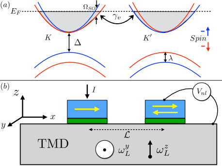
Figure 1: (Color online) (a) The energy spectrum of TMD at $K$ and $K^{\prime}$ valleys is shown schematically. In n-type material the states with energies below $E_{F}$ are occupied. The splitting between the $\uparrow$ and $\downarrow$ branches at the Fermi level is $\Omega_{\scriptscriptstyle SO}=\big{(}\frac{\lambda}{\Delta}\big{)}E_{F}$ and is much smaller than $E_{F}$. Short-range impurities are responsible for intervalley scattering with a rate $\gamma_{v}$. (b) Schematic illustration of the spin-transport experiment in TMD. The measure of the nonlocal resistance is a voltage between the channel and the right ferromagnet detector generated upon injecting the current through the left ferromagnetic electrode. Injector and detector shown in blue are separated from the channel by a tunnel barrier shown in green. While the injected polarized electrons travel either in the valley $K$ or in the valley $K^{\prime}$, their spin precesses in the effective field ${\bm{\omega}}_{L}+{\hat{z}}\Omega_{\scriptscriptstyle SO}$ or ${\bm{\omega}}_{L}-{\hat{z}}\Omega_{\scriptscriptstyle SO}$. As a result of intervalley scattering, the spin dynamics is described by a system of the coupled equations Eq. (III). We study the limit of a small, compared to the diffusion length, distance ${\cal L}$ between injector and detector. The specifics of TMDs is that for external field, ${\bm{\omega}}_{L}$, oriented along $z$ and $y$ the shapes of the Hanle curves $V_{nl}(\omega_{L})$ are completely different.

I Introduction

Transition-metal dichalcogenides (TMDs) in a 2D domain are single-layer semiconductors with lattice similar to graphene. Unlike graphene, they possess a bandgap, which makes them attractive for optoelectronic applications, such as field-effect transistorTransistor1 ; Transistor2 , see e.g. Ref. Review, for review. Unlike graphene, the electron states in $K$ and $K^{\prime}$ valleys are not equivalent. This inequivalence is owed to the spin-orbit coupling. The $K$ and $K^{\prime}$ wave functions corresponding to the same momenta and energies differ by the spin direction. Spin-orbit splitting of the conduction band is much smaller than that of the valence band.KP1 ; KP2 ; KP3 ; KP4 ; KP5 ; KP6 ; KP7 As a result of the band splitting, there are two excitons in a given valley. Correspondingly, in undoped samples, the spectra of the exciton absorption, reflection, and luminescence exhibit a two-peak structure, as was demonstrated experimentally by many groupsOpticalExperimentHeinz ; OpticalExperimentNatureNano ; OpticalExperimentNaturePhysics ; OpticalHanleNatureCobden ; ClassicalHeinz1 ; ClassicalHeinz2 ; Biexciton ; IntervalleyPump ; Glazov2 ; Glazov3

Upon photoexcitation of n-type samples, generated holes rapidly recombine with resident electrons, while generated electrons preserve spin memory for rather long times $\sim 1$ns. This was established in Refs. Crooker1, ; Crooker3, on the basis of the analysis of the Hanle-Kerr data is magnetic field parallel to the layer. The fact that the optical response is sensitive to a magnetic field of $\sim 50$mT which is much smaller than the effective spin-orbit (SO) field seems rather unusual. The explanation for that suggested in Ref. Crooker1, is based on the fact that an electron, created by light, undergoes fast inter-valley scattering, which effectively averages out the SO field. This scattering is facilitated by disorder, unlike the intervalley scattering of excitonsGlazov1 ; Wu1 which is facilitated by the exchange interaction. The latter mechanism is similar to the non-radiative Förster energy transfer. Optical response to a magnetic field perpendicular to the layer emerges only when the field is very strongCrooker2 $\sim 50$T.

Gate voltagesGate can control the type and the concentration of carriers in TMDs. However, the transport measurements reported to date are scarce compared to the optical studies. The highest mobility reported to dateHighMobilityNatureLett in n-type MoS₂ is $\sim 10^{3}$cm²/Vs. For most samples the mobility is lowerHighMobilityNature $\sim 10^{2}$cm²/Vs. The fact that it depends on temperatureHighMobilityNatureLett ; HighMobilityNature suggests that the electron states are not far from the metal-insulator transition. Hopping transport has also been reported in disordered MoS₂ samples.Hopping

Spin transport has never been studied in TMDsfootnote . On the other hand, relatively low mobility does not prevent such studies, see e.g. Ref. TiwariZnO, . Note that the spin transport and the Kerr rotation signals are both limited by the spin-memory loss of carriers. In this regard, the most interesting question is how the spin dynamics of electrons reflected in the spin transport in n-type TMDs is related to the spin dynamics of excitons inferred from the Hanle-Kerr measurementsCrooker1 ; Crooker3 . This issue is studied theoretically in the present paper. One cannot expect an observable spin transport in p-type TMDs. The separation of $\sim 150$meV between the tops of $\uparrow$ and $\downarrow$ bands in each valley suggests that “intrinsic” spin precession is too fast. Intervalley scattering is also strictly forbidden unless phonons are involvedDery1 ; Dery2 .

There are apparent differences between the spin-transport studies and polarization-of-luminescence techniques. Firstly, the optical experiments reveal the dynamics of the $z$-component of spin, $S_{z}(t)$, while conventional spin transport measures $S_{x}(t)$, $S_{y}(t)$, as illustrated in the Fig. 1. Secondly, the magnitude of the SO field in the metallic regime depends strongly on the electron density and is much smaller than for the excitons. It is also nontrivial that the electron inter-valley scattering rate, $\gamma_{v}$, depends on the concentration of the short-range impurities (defectsDefects ) allowing the large momentum transfer between the valleys. Finally, the Förster-like mechanism, which is at work for excitons, does not apply for two Fermi seas at $K$ and $K^{\prime}$ valleys. As for relation between the spin transport and the Kerr rotation techniques, the latter also studies $S_{z}(t)$. Besides, the Kerr rotation signal is pronounced for probe frequencies near the A-exciton resonanceCrooker1 ; Crooker3 not at the Fermi level.

We will demonstrate that the shapes of the transport Hanle curves in TMDs depend dramatically on the ratio of $\gamma_{v}$ to the SO splitting of the electron spectrum, $\Omega_{\scriptscriptstyle SO}$, and that these shapes are different from the conventional transport Hanle curves. In this regard, we emphasize, that the shapes of the Hanle curves reported for wide variety of materials are very robustRobust . Specifics of the Hanle curves in TMDs is due to the valley asymmetry.

We show that, unlike conventional materials, the shape of the transport Hanle curve in TMDs depends on the orientation of the external field. If the spin polarization of electrons injected from a ferromagnet is along the $x$-axis, see Fig. 1, the dynamics of the injected spin is different for the external field parallel to the layer (along $y$) or normal to the layer (along $z$). For normal orientation and $\gamma_{v}\ll\Omega_{\scriptscriptstyle SO}$ this dynamics is different for different valleys. As a result, of this the Hanle curve has a two-peak structure. A distinct Hanle shape also persists for the normal orientation when $\gamma_{v}\gg\Omega_{\scriptscriptstyle SO}$. It represents the difference of two conventional Hanle profiles with very different widths: the wider reflecting the valley-symmetric mode of the overdamped spin dynamics, while the narrower reflecting the valley-antisymmetric mode.

When the external field is parallel to the layer, the Hanle curve has a singularity at a zero field. This singularity is due to the valley-asymmetric mode describing the slow time decay of the spin density. The decay is slow as a result of fast alternation of valleys; external field is responsible for coupling of the initial spin distribution to this mode. Characteristic width of the Hanle curve for the parallel orientation of external field is much smaller than for normal orientation. This is in accord with results experimental findingsCrooker1 ; Crooker3 ; Crooker2 for magnetic-field response of photoexcited carriers, and is not surprising, since the spin dynamics for electrons and excitons are qualitatively similar.

II Density dependence of the SO splitting of the electron spectrum

The ${\bm{k}}\cdot{\bm{p}}$ Hamiltonian of a TMD, established in Ref. Hamiltonian, , see also Refs. KP1, ; KP2, ; KP3, ; KP4, ; KP5, ; KP6, ; KP7, , contains three energies, namely, the gap, $\Delta$, the hopping integral, $t$, and the SO-induced spin splitting of the valence band top, $2\lambda$. With two valleys coupled to two spin projections, it represents a $4\times 4$ matrix. In the presence of external field having $y$ and $z$ components, this matrix has the form

$$H=\begin{pmatrix}\frac{\Delta}{2}+\omega_{L}^{z}&at\tau ke^{-i\theta\tau}&-i\omega_{L}^{y}&0\\ at\tau ke^{i\theta\tau}&-\frac{\Delta}{2}+\omega_{L}^{z}+\lambda\tau&0&-i\omega_{L}^{y}\\ i\omega_{L}^{y}&0&\frac{\Delta}{2}-\omega_{L}^{z}&at\tau ke^{-i\theta\tau}\\ 0&i\omega_{L}^{y}&at\tau ke^{i\theta\tau}&-\frac{\Delta}{2}-\omega_{L}^{z}-\lambda\tau\end{pmatrix},$$ (1)

where $a$ is the lattice constant, $\omega_{L}^{y}$ and $\omega_{L}^{z}$ are the corresponding Zeeman energies, $k$ and $\theta$ are the magnitude and the orientation of the wave vector. The valley index $\tau$ takes the values $\pm 1$.

The spectrum, $\varepsilon(k)$, originating from the Hamiltonian Eq. (3) is the solution of the fourth-order equation

$$\Big{[}\big{(}\varepsilon+\frac{\Delta}{2}+\omega_{L}^{z}+\lambda\tau\big{)}\big{(}\varepsilon-\frac{\Delta}{2}+\omega_{L}^{z}\big{)}-(atk)^{2}\Big{]}$$

$$\times \Big{[}\big{(}\varepsilon+\frac{\Delta}{2}-\omega_{L}^{z}-\lambda\tau\big{)}\big{(}\varepsilon-\frac{\Delta}{2}-\omega_{L}^{z}\big{)}-(atk)^{2}\Big{]}$$

$$= \Big{[}2\varepsilon^{2}+2\big{(}\frac{\Delta}{2}\big{)}^{2}+2(atk)^{2}-(\omega_{L}^{z})^{2}-(\omega_{L}^{z}+\lambda\tau)^{2}\Big{]}(\omega_{L}^{y})^{2}.$$ (2)

In the absence of magnetic field the right-hand side is zero, and each bracket in the left-hand side determines the corresponding branch of the spectrum. With magnetic field, we can find the spectrum of the conduction band perturbatively in the small parameter $\omega_{L}^{y}/\Delta$. The result reads

$$\varepsilon(k)=\frac{\Delta}{2}+\frac{\hbar k^{2}}{2m_{c}}\pm\sqrt{\Big{[}\omega_{L}^{z}+\Big{(}\frac{\lambda\tau}{\Delta}\Big{)}\frac{\hbar k^{2}}{2m_{c}}\Big{]}^{2}+(\omega_{L}^{y})^{2}}.$$ (3)

Here $m_{c}=\Delta\hbar/2a^{2}t^{2}$ is the effective mass of the conduction-band electron. Relative splitting of $\uparrow$ and $\downarrow$ branches is always small by virtue of the parameter $\lambda/\Delta$, which is $\approx 0.1$ for MoS₂. The above result has a simple interpretation. Namely, $\Omega_{\scriptscriptstyle SO}$ acts as an effective field directed along $z$ which assumes opposite values for two the valleys.

In n-type TMDs the electron states with $k<k_{\scriptscriptstyle F}$, where $k_{\scriptscriptstyle F}$ is the Fermi momentum, are occupied. The parameter crucial for spin transport is the ratio, $\gamma_{v}/\Omega_{\scriptscriptstyle SO}$, of the intervalley scattering rate and the band splitting,footnote2 $\Omega_{\scriptscriptstyle SO}=\left(\frac{\lambda}{\Delta}\right)E_{\scriptscriptstyle F}$, at the Fermi level $E_{\scriptscriptstyle F}=\hbar k_{\scriptscriptstyle F}^{2}/2m_{c}$. We can perform a numerical estimate of this ratio assuming that the mobility is limited by the same short-range impurities that are responsible for intervalley scattering. The fact that point-like defects are the leading source of scattering in TMDs is commonly accepted, see e.g. Ref. Defects, . With mobility given by $\mu=\frac{e}{m_{c}\gamma_{v}}$ and $k_{\scriptscriptstyle F}^{2}=4\pi n$, where $n$ is the electron density, we find

$$\Gamma=\frac{\gamma_{v}}{\Omega_{\scriptscriptstyle SO}}=\left(\frac{\Delta}{\lambda}\right)\frac{e}{2\pi\hbar\mu n}.$$ (4)

For numerical estimate we choose a typical value $n=10^{13}cm^{-2}$. Then for the highest reported mobilityHighMobilityNatureLett for electrons in MoS₂, $\mu=10^{3}cm^{2}/Vs$, the ratio Eq. (4) is equal to $0.2$, while for typical mobilityHighMobilityNature $\mu=10^{2}cm^{2}/Vs$ it is $10$ times bigger. Thus, we conclude that both regimes $\Gamma\ll 1$ and $\Gamma\gg 1$ are viable for spin transport.

III Nonlocal resistance

Once the spectrum Eq. (3) in magnetic field is known and the intervalley scattering rate is introduced, the procedure of calculation of nonlocal resistance is straightforward. vanWeesPioneering First the splitting of the spectrum is incorporated into the equation of the dynamics for the spin density ${\bm{S}}(t)$ which is solved with an initial condition ${\bm{S}}(0)={\hat{x}}$. Then the solution for $S_{x}(t)$ is multiplied by the diffusion propagator

$$P_{{\cal L}}(t)=\frac{1}{\left(4\pi Dt\right)^{1/2}}\exp\left(-\frac{{\cal L}^{2}}{4Dt}\right),$$ (5)

where ${\cal L}$ is the distance between the injector and detector and $D$ is the diffusion coefficient related to mobility via the Einstein relation. Finally, the nonlocal resistance is obtained by integration over time

$$R(\omega_{L})={\cal R}_{0}\int\limits_{0}^{\infty}dtS_{x}(t)P_{{\cal L}}(t),$$ (6)

where ${\cal R}_{0}$ is the prefactor. The specifics of TMDs is that $S_{x}(t)$ is the sum $S_{x}(t)=S_{x}^{K}(t)+S_{x}^{K^{\prime}}(t)$ of contributions of the two inequivalent valleys, so that the spin dynamics is governed by the system of the coupled equationsCrooker1 ; footnote1

$$\frac{d{\bm{S}}^{K}}{dt} =\omega_{L}^{y}{\hat{y}}\times{\bm{S}}^{K}+(\Omega_{\scriptscriptstyle SO}+\omega_{L}^{z}){\hat{z}}\times{\bm{S}}^{K}-\gamma_{v}\left({\bm{S}}^{K}-{\bm{S}}^{K^{\prime}}\right),$$

$$\frac{d{\bm{S}}^{K^{\prime}}}{dt} =\omega_{L}^{y}{\hat{y}}\times{\bm{S}}^{K^{\prime}}-(\Omega_{\scriptscriptstyle SO}-\omega_{L}^{z}){\hat{z}}\times{\bm{S}}^{K^{\prime}}+\gamma_{v}\left({\bm{S}}^{K}-{\bm{S}}^{K^{\prime}}\right).$$ (7)

We will consider the cases of the normal, $\omega_{L}\parallel z$, and tangential, $\omega_{L}\parallel y$, orientations of the external field separately.

Figure 2: (Color online) Nonlocal resistance calculated from Eqs. (VI), (VI) is plotted versus the dimensionless magnetic field normal to the plane for different intervalley scattering rates (in the units of $\Omega_{\scriptscriptstyle SO}$): $\Gamma=0.2$ (a), $\Gamma=0.7$ (b), $\Gamma=1.2$ (c), and $\Gamma=1.8$ (d). Two-peak structure of the Hanle curves centered at $\omega_{L}^{z}=\pm\Omega_{\scriptscriptstyle SO}$ evolves with increasing $\Gamma$ to a conventional Hanle shape.

IV Normal orientation of the external field

For normal orientation, the $z$-component of the spin drops out from the system Eq. (III). To analyze this system, it is convenient, following Ref. Crooker1, , to introduce, in addition to the net spin projections $S_{x}(t)$ and $S_{y}(t)$, the valley imbalances

$$S_{x}^{-}=S_{x}^{K}-S_{x}^{K^{\prime}},~{}~{}~{}~{}S_{y}^{-}=S_{y}^{K}-S_{y}^{K^{\prime}}.$$ (8)

Upon the Laplace transform, the system of four equations for $S_{x}$, $S_{y}$, $S_{x}^{-}$, and $S_{y}^{-}$ assumes the form

$$p{\tilde{S}}_{x}-1 =-\Omega_{\scriptscriptstyle SO}{\tilde{S}}_{y}^{-}-\omega_{L}^{z}{\tilde{S}}_{y}$$

$$p{\tilde{S}}_{y} =\Omega_{\scriptscriptstyle SO}{\tilde{S}}_{x}^{-}+\omega_{L}^{z}{\tilde{S}}_{x}$$

$$p_{1}{\tilde{S}}_{x}^{-} =-\Omega_{\scriptscriptstyle SO}{\tilde{S}}_{y}-\omega_{L}^{z}{\tilde{S}}_{y}^{-}$$

$$p_{1}{\tilde{S}}_{y}^{-} =\Omega_{\scriptscriptstyle SO}{\tilde{S}}_{x}+\omega_{L}^{z}{\tilde{S}}_{x}^{-},$$ (9)

where ${\tilde{S}}(p)$ stands for the Laplace-transformed $S(t)$, and $p_{1}$ is defined as

$$p_{1}=p+2\gamma_{v}.$$ (10)

The solution of the system for ${\tilde{S}}_{x}$ reads

$${\tilde{S}}_{x}=\frac{pp_{1}^{2}+p(\omega_{L}^{z})^{2}+p_{1}\Omega_{\scriptscriptstyle SO}^{2}}{(pp_{1})^{2}+2pp_{1}\Omega_{\scriptscriptstyle SO}^{2}+(p^{2}+p_{1}^{2})(\omega_{L}^{z})^{2}+[\Omega_{\scriptscriptstyle SO}^{2}-(\omega_{L}^{z})^{2}]^{2}}.$$ (11)

Four frequencies of the modes describing the spin dynamics are determined by the zeros of the denominator. They are given by

$$p=\Omega_{\scriptscriptstyle SO}\Big{[}-\Gamma\pm i\Big{(}\frac{\omega_{L}^{z}}{\Omega_{\scriptscriptstyle SO}}\pm\sqrt{1-\Gamma^{2}}\Big{)}\Big{]},$$ (12)

where the parameter $\Gamma$ is the dimensionless intervalley scattering rate defined by Eq. (4).

It is seen from Eq. (12) that the spin dynamics depends dramatically on the value of $\Gamma$. For $\Gamma\ll 1$ there are two different oscillation frequencies, $\Omega_{\scriptscriptstyle SO}\pm\omega_{L}^{z}$, which decay with the same rate, $\gamma_{v}$. On the contrary, for $\Gamma\gg 1$ both frequencies are equal to $\omega_{L}^{z}$, but the decay rates are very different. For the valley-symmetric mode it is equal to $2\gamma_{v}$, while the valley-antisymmetric mode decays very slowly with the Dyakonov-Pereldyakonov-perel rate $\approx\Omega_{\scriptscriptstyle SO}^{2}/2\gamma_{v}$. The time evolution of $S_{x}(t)$ has different forms for $\Gamma<1$ and $\Gamma>1$. Namely, for $\Gamma<1$ this evolution is given by

$$S_{x}(t)= \frac{1}{2}\Bigg{\{}\frac{\Gamma}{\sqrt{1-\Gamma^{2}}}\Bigg{[}\sin\Bigg{(}\Big{(}\frac{\omega_{L}^{z}}{\Omega_{\scriptscriptstyle SO}}+\sqrt{1-\Gamma^{2}}\Big{)}\Omega_{\scriptscriptstyle SO}t\Bigg{)}$$

$$- \sin\Bigg{(}\Big{(}\frac{\omega_{L}^{z}}{\Omega_{\scriptscriptstyle SO}}-\sqrt{1-\Gamma^{2}}\Big{)}\Omega_{\scriptscriptstyle SO}t\Bigg{)}\Bigg{]}$$

$$+ \Bigg{[}\cos\Bigg{(}\Big{(}\frac{\omega_{L}^{z}}{\Omega_{\scriptscriptstyle SO}}+\sqrt{1-\Gamma^{2}}\Big{)}\Omega_{\scriptscriptstyle SO}t\Bigg{)}$$

$$+ \cos\Bigg{(}\Big{(}\frac{\omega_{L}^{z}}{\Omega_{\scriptscriptstyle SO}}-\sqrt{1-\Gamma^{2}}\Big{)}\Omega_{\scriptscriptstyle SO}t\Bigg{)}\Bigg{]}\Bigg{\}}\exp\Big{[}-\Gamma\Omega_{\scriptscriptstyle SO}t\Big{]},$$ (13)

while for $\Gamma>1$ we have

$$S_{x}(t)=\frac{1}{2}\Bigg{\{}\Big{(}1+\frac{\Gamma}{\sqrt{\Gamma^{2}-1}}\Big{)}\exp\Big{[}-\Big{(}\Gamma-\sqrt{\Gamma^{2}-1}\Big{)}\Omega_{\scriptscriptstyle SO}t\Big{]}$$

$$+ \Big{(}1-\frac{\Gamma}{\sqrt{\Gamma^{2}-1}}\Big{)}\exp\Big{[}-\Big{(}\Gamma+\sqrt{\Gamma^{2}-1}\Big{)}\Omega_{\scriptscriptstyle SO}t\Big{]}\Bigg{\}}\cos\omega_{L}^{z}t.$$ (14)

V External field along ${\hat{y}}$

For parallel magnetic field, there are, in general, six modes of the spin dynamics. Although the spin dynamics in this geometry was considered in Ref. Crooker1, , only the time evolution of $S_{z}$ was studied, while we are interested in $S_{x}(t)$, $S_{y}(t)$. It turns out that the frequencies for $S_{x}(t)$ are the same as for $S_{z}(t)$, while for $S_{y}(t)$ they are completely different. This is certainly the specifics of TMDs.

The field along ${\hat{y}}$ couples $S_{x}(t)$ and $S_{z}(t)$ via the conventional Larmor precession. In addition, the valley-asymmetric field $\pm{\hat{z}}\Omega_{\scriptscriptstyle SO}$ couples $S_{x}(t)$ to the spin imbalance, $S_{y}^{-}$. As a result, the system $6\times 6$ decouples into two systems $3\times 3$. The Laplace-transformed system involving ${\tilde{S}}_{x}$ reads

$$p{\tilde{S}}_{x}-1 =-\Omega_{\scriptscriptstyle SO}{\tilde{S}}_{y}^{-}+\omega_{L}^{y}{\tilde{S}}_{z}$$

$$p{\tilde{S}}_{z} =-\omega_{L}^{y}{\tilde{S}}_{x}$$

$$p_{1}{\tilde{S}}_{y}^{-} =\Omega_{\scriptscriptstyle SO}{\tilde{S}}_{x},$$ (15)

By contrast to the normal orientation, the solution

$${\tilde{S}}_{x}=\frac{pp_{1}}{p^{2}p_{1}+p_{1}(\omega_{L}^{y})^{2}+p\Omega_{\scriptscriptstyle SO}^{2}}$$ (16)

contains a third-order polynomial in the denominator. With regard to sensitivity of the spin dynamics to the external field, the most interesting case is $\Gamma\gg 1$, when the intervalley scattering is fast. In this limit, the expressions for the two poles have a simple form

$$p=\Omega_{\scriptscriptstyle SO}\Bigg{[}-\frac{1}{4\Gamma}\pm\sqrt{\Big{(}\frac{1}{4\Gamma}\Big{)}^{2}-\Big{(}\frac{\omega_{L}^{y}}{\Omega_{\scriptscriptstyle SO}}\Big{)}^{2}}\Bigg{]},$$ (17)

and reproduce the corresponding frequencies obtained in Ref. Crooker1, . Expression Eq. (17) defines a small characteristic magnetic field, $\omega_{L}^{y}\sim\Omega_{\scriptscriptstyle SO}/\Gamma$, which is the inverse Dyakonov-Perel relaxation time. In the same limit, $\Gamma\gg 1$, the third frequency is given by

$$p=\Omega_{\scriptscriptstyle SO}\Bigg{[}-2\Gamma+\frac{2\Gamma}{4\Gamma^{2}+\Big{(}\frac{\omega_{L}^{y}}{\Omega_{\scriptscriptstyle SO}}\Big{)}^{2}}\Bigg{]}.$$ (18)

It corresponds to the decay with the rate $2\gamma_{v}$ and is insensitive to weak magnetic fields.

As magnetic field increases, the argument of the square root in Eq. (17) changes sign. This is reflected in the spin dynamics, which is different for $\omega_{L}^{y}$ bigger and smaller than $\Omega_{\scriptscriptstyle SO}/4\Gamma$. At low fields we have

$$S_{x}(t)= \frac{1}{2}\Bigg{[}\Bigg{(}1+\frac{1}{\sqrt{1-\big{(}\frac{4\omega_{L}^{y}\Gamma}{\Omega_{\scriptscriptstyle SO}}\big{)}^{2}}}\Bigg{)}$$

$$\times \exp\Bigg{[}-\Bigg{(}\frac{1}{4\Gamma}+\sqrt{\Big{(}\frac{1}{4\Gamma}\Big{)}^{2}-\Big{(}\frac{\omega_{L}^{y}}{\Omega_{\scriptscriptstyle SO}}\Big{)}^{2}}\Bigg{)}\Omega_{\scriptscriptstyle SO}t\Bigg{]}$$

$$+ \Bigg{(}1-\frac{1}{\sqrt{1-\big{(}\frac{4\omega_{L}^{y}\Gamma}{\Omega_{\scriptscriptstyle SO}}\big{)}^{2}}}\Bigg{)}$$

$$\times \exp\Bigg{[}-\Bigg{(}\frac{1}{4\Gamma}-\sqrt{\Big{(}\frac{1}{4\Gamma}\Big{)}^{2}-\Big{(}\frac{\omega_{L}^{y}}{\Omega_{\scriptscriptstyle SO}}\Big{)}^{2}}\Bigg{)}\Omega_{\scriptscriptstyle SO}t\Bigg{]},$$ (19)

i.e. the dynamics is overdamped. It becomes oscillatory for $\omega_{L}^{y}>\Omega_{\scriptscriptstyle SO}/4\Gamma$. In this domain we find

$$S_{x}(t)= \exp\Big{[}-\frac{\Omega_{\scriptscriptstyle SO}}{4\Gamma}t\Big{]}\Bigg{[}\cos\Bigg{(}\sqrt{\Big{(}\frac{\omega_{L}^{y}}{\Omega_{\scriptscriptstyle SO}}\Big{)}^{2}-\Big{(}\frac{1}{4\Gamma}\Big{)}^{2}}\Omega_{\scriptscriptstyle SO}t\ \Bigg{)}$$

$$- \frac{1}{\sqrt{\big{(}\frac{4\omega_{L}^{y}\Gamma}{\Omega_{\scriptscriptstyle SO}}\big{)}^{2}-1}}\sin\Bigg{(}\sqrt{\Big{(}\frac{\omega_{L}^{y}}{\Omega_{\scriptscriptstyle SO}}\Big{)}^{2}-\Big{(}\frac{1}{4\Gamma}\Big{)}^{2}}\Omega_{\scriptscriptstyle SO}t\ \Bigg{)}\Bigg{]}.$$ (20)

Compared to Ref. Crooker1, , where $S_{z}(t)$ was calculated, the amplitudes of the harmonics in Eq. (V) are different.

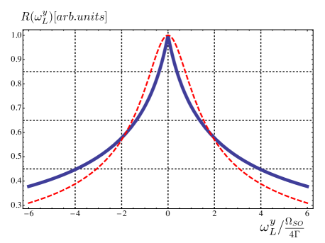
Figure 3: (Color online) Universal shape of the Hanle curve, $R(4\omega_{L}^{y}\Gamma/\Omega_{\scriptscriptstyle SO})$, for the parallel orientation of the magnetic field is plotted from Eq. (25). A cusp at zero field reflects the slow-decaying valley-asymmetric mode of the spin dynamics. For comparison, the conventional Hanle curve Eq. (22) is plotted with dashed line.

VI Shapes of the Hanle curves

To find the Hanle profiles for normal orientation of magnetic field one should substitute Eqs. (IV) and (IV) into Eq. (6) and perform the integration over time. The structure of $S_{x}(t)$, sinusoidal function times exponential decay, suggests that the integration can be carried out analyticallySilsbee1985 ; Silsbee1988 for arbitrary ${\cal L}$ . However, in samples with low mobility, the regime of small distance, ${\cal L}$, between injector and detector is most relevant. This is because the diffusion time, ${\cal L}^{2}/D$, should not exceed much the spin relaxation time. Upon setting ${\cal L}=0$ in $P_{\cal L}(t)$ Eq. (5) the integration is easily performed with the help of the relations

$$\int\limits_{0}^{\infty}\frac{dt~{}e^{-vt}}{\sqrt{t}}\sin(ut) =\text{sign}(u)\sqrt{\frac{\pi}{2v}}\mathrm{F}\Big{(}\frac{u}{v}\Big{)},$$

$$\int\limits_{0}^{\infty}\frac{dt~{}e^{-vt}}{\sqrt{t}}\cos(ut) =\sqrt{\frac{\pi}{2v}}\mathrm{G}\Big{(}\frac{u}{v}\Big{)},$$ (21)

where the functions $\mathrm{F}(z)$ and $\mathrm{G}(z)$ are defined as

$$\mathrm{F}\big{(}z\big{)}=\frac{\sqrt{\sqrt{1+z^{2}}-1}}{\sqrt{1+z^{2}}},~{}~{}~{}~{}~{}\mathrm{G}\big{(}z\big{)}=\frac{\sqrt{\sqrt{1+z^{2}}+1}}{\sqrt{1+z^{2}}}.$$ (22)

The expressions for nonlocal resistance in the $\perp$ geometry can be now expressed via the functions $\mathrm{F}$ and $\mathrm{G}$. For $\Gamma<1$ we have

$$R(\omega_{L}^{z}) =\frac{{\cal R}_{0}}{4\sqrt{2D\Omega_{\scriptscriptstyle SO}\Gamma}}$$

$$\times\Bigg{\{}\mathrm{G}\Big{(}\frac{\omega_{L}^{z}}{\Omega_{\scriptscriptstyle SO}\Gamma}+\sqrt{\frac{1}{\Gamma^{2}}-1}\Big{)}+\mathrm{G}\Big{(}\frac{\omega_{L}^{z}}{\Omega_{\scriptscriptstyle SO}\Gamma}-\sqrt{\frac{1}{\Gamma^{2}}-1}\Big{)}$$

$$+\frac{\Gamma}{\sqrt{1-\Gamma^{2}}}$$

$$\times\Bigg{[}\text{sign}\Big{[}\big{(}\frac{\omega_{L}^{z}}{\Omega_{\scriptscriptstyle SO}}+\sqrt{1-\Gamma^{2}}\big{)}\Omega_{\scriptscriptstyle SO}\Big{]}\mathrm{F}\Big{(}\frac{\omega_{L}^{z}}{\Omega_{\scriptscriptstyle SO}\Gamma}+\sqrt{\frac{1}{\Gamma^{2}}-1}\Big{)}$$

$$-\text{sign}\Big{[}\big{(}\frac{\omega_{L}^{z}}{\Omega_{\scriptscriptstyle SO}}-\sqrt{1-\Gamma^{2}}\big{)}\Omega_{\scriptscriptstyle SO}\Big{]}\mathrm{F}\Big{(}\frac{\omega_{L}^{z}}{\Omega_{\scriptscriptstyle SO}\Gamma}-\sqrt{\frac{1}{\Gamma^{2}}-1}\Big{)}\Bigg{]}\Bigg{\}}.$$ (23)

The corresponding expression for $\Gamma>1$ reads

$$R(\omega_{L}^{z}) =\frac{{\cal R}_{0}}{4\sqrt{2D\Omega_{\scriptscriptstyle SO}(\Gamma^{2}-1)}}$$

$$\times\Bigg{[}\frac{1}{\Big{(}\Gamma-\sqrt{\Gamma^{2}-1}\Big{)}^{3/2}}\mathrm{G}\Bigg{(}\frac{\omega_{L}^{z}}{\Omega_{\scriptscriptstyle SO}}\Big{(}\Gamma+\sqrt{\Gamma^{2}-1}\Big{)}\Bigg{)}$$

$$-\frac{1}{\Big{(}\Gamma+\sqrt{\Gamma^{2}-1}\Big{)}^{3/2}}\mathrm{G}\Bigg{(}\frac{\omega_{L}^{z}}{\Omega_{\scriptscriptstyle SO}}\Big{(}\Gamma-\sqrt{\Gamma^{2}-1}\Big{)}\Bigg{)}\Bigg{]}.$$ (24)

Evolution of the shape of the Hanle curves with $\Gamma$ described by Eqs. (VI), (VI) is the following. For slow intervalley scattering $R(\omega_{L}^{z})$ exhibits a two-peak structure with maxima at $\omega_{L}^{z}\approx\pm\Omega_{\scriptscriptstyle SO}$. Each peak corresponds to the “compensation” of the SO-splitting in a given valley by the external field. The widths of the peaks are $\sim\gamma_{v}$. For $\Gamma\approx 0.7$ the peaks merge, and, upon further increase of $\Gamma$, transform into the difference of the two peaks with small, $\sim\Omega_{\scriptscriptstyle SO}/\Gamma$, and big, $\sim\Omega_{\scriptscriptstyle SO}\Gamma$, widths centered at $\Omega_{L}^{z}=0$. The broad peak, however, has a much smaller magnitude. So the shape for $\Gamma\gg 1$ is, essentially, the conventional Hanle shape with width determined by the inverse Dyakonov-Perel relaxation time. The evolution of $R(\omega_{L}^{z})$ with $\Gamma$ is illustrated in Fig. 2.

Turning to the geometry with external field along ${\hat{y}}$, we first observe that $S_{x}(t)$ given by Eqs. (V), (V) contains only one scale of $\omega_{L}^{y}$, namely, $\omega_{L}^{y}=\Omega_{\scriptscriptstyle SO}/\Gamma$. Since we assumed fast intervalley scattering, this characteristic field is much smaller than the splitting $\Omega_{\scriptscriptstyle SO}$. Naturally, the Hanle curve is a function of a single parameter $\omega_{L}^{y}\Gamma/\Omega_{\scriptscriptstyle SO}$. The form of this function can be found using the identities Eq. (VI). While the integrands in Eq. (6) are different for $\omega_{L}^{y}<\Omega_{\scriptscriptstyle SO}/4\Gamma$ and $\omega_{L}^{y}>\Omega_{\scriptscriptstyle SO}/4\Gamma$, the resulting shape is given by a single concise expression

$$R(\omega_{L}^{y})=\frac{{\cal R}_{0}}{\sqrt{2D\Omega_{\scriptscriptstyle SO}}}\frac{\Gamma}{\sqrt{1+\big{|}\frac{4\omega_{L}^{z}\Gamma}{\Omega_{\scriptscriptstyle SO}}\big{|}}}.$$ (25)

The Hanle curve in the form of Eq. (25) falls off with magnetic field as $1/\sqrt{\omega_{L}^{y}}$, i.e. in the same way as a regular Hanle curve. However, it exhibits a unique feature at small field, where the slope has an abrupt cusp, see Fig. 3. The origin of the cusp can be traced to the second term in Eq. (V). Rather than spin precession, this term describes the slow decay, as $\exp(-|\omega_{L}^{y}|t)$, of the spin density. This slow decay reveals the specifics of the two-valley spin dynamics Eq. (V), for which the valley-asymmetric mode decays anomalously slow.

VII Concluding remarks

(i) In optics experiments the valleys were “addressed” separately, in the sense, that, for a given frequency, different polarizations of light generated excitons in different valleys. Conventional spin transport is valley-insensitive. On the other hand, the spin-pumping setupTserkovnyak can serve as an analog of optical selective valley excitation. Assume that the ferromagnetic resonance is excited in the ferromagnet which injects spin into a TMD layer. The pumped spin current would flow in one of the valleys depending on polarization of the microwave field exciting the resonance. The analogy between the selective valley excitation in optics and by the spin pumping is straightforward. While in optical experiments an absorbed photon generates an electron in the conduction band and a hole in the valence band, in spin pumping it is a magnon that creates an electron-hole pair in the Fermi sea of the conduction band.

(ii) For fast intervalley scattering, the slow-decaying modes of the spin dynamics are present for both orientations of the external field. These modes are valley-asymmetric and originate from almost complete compensation of the SO field, $\Omega_{\scriptscriptstyle SO}$, in the valley $K$ and $-\Omega_{\scriptscriptstyle SO}$ in the valley $K^{\prime}$. However, the decay rates of these modes are drastically different in weak external field. This is because, for $\perp$ orientation, the result of compensation is simply the external field ${\hat{z}}\omega_{L}^{z}$, while, for $\parallel$ orientation, the result of compensation of ${\hat{y}}\omega_{L}^{y}+{\hat{z}}\Omega_{\scriptscriptstyle SO}$ and ${\hat{y}}\omega_{L}^{y}-{\hat{z}}\Omega_{\scriptscriptstyle SO}$ is only quadratic in external field. Then the prime effect of the external field on the spin-dynamics is the field-dependent decay.

(iii). Measuring the Hanle curves in both $\parallel$ and $\perp$ orientations allows, in principle, to determine the values of both relevant parameters, $\Omega_{\scriptscriptstyle SO}$ and $\gamma_{v}$.

(iv). Our main results Eqs. (VI), Eq. (VI), and Eq. (25 were derived in the limit of small distance ${\cal L}$ between injector and detector. Now we can quantify the corresponding condition. Characteristic magnetic field in Eq. (25) is $\omega_{L}^{y}\sim\Omega_{\scriptscriptstyle SO}/\Gamma$. Thus, the diffusion time, ${\cal L}^{2}/D$ should be smaller than the precession time, i.e. ${\cal L}\ll\Big{(}D\Gamma/\Omega_{\scriptscriptstyle SO}\Big{)}^{1/2}$. In the opposite limit the Hanle curve exhibits sensitivity to even weaker fields. The corresponding expression for nonlocal resistance in this limit can be cast in the form

$$\frac{R(\omega_{L}^{y})-R(0)}{R(0)}=-\frac{2|\omega_{L}^{y}|\Gamma}{\Omega_{\scriptscriptstyle SO}}\exp\Big{[}-2|\omega_{L}^{y}|\Big{(}\frac{{\cal L}^{2}\Gamma}{D\Omega_{\scriptscriptstyle SO}}\Big{)}^{\frac{1}{2}}\Big{]}.$$ (26)

This result suggests that the Hanle curve has a minimum at zero field and two maxima at $\omega_{L}^{y}=\pm\Big{(}D\Omega_{\scriptscriptstyle SO}/4{\cal L}^{2}\Gamma\Big{)}^{1/2}$ much smaller than $\Omega_{\scriptscriptstyle SO}/\Gamma$.

(v) In experimental paper Ref. Crooker2, the sensitivity of the optical response to the normal magnetic field was not registered until $\omega_{L}^{z}$ was as high as $65$T. We, on the other hand, predict the sensitivity of the spin transport to much weaker fields. The reason is that $z$-projection of spin, $S_{z}(t)$, registered in optical experiments, drops out from the equations Eq. (IV) for the spin dynamics in $\perp$ orientation, whereas the dynamics, $S_{x}(t)$, relevant for spin transport, persists.

(vi) Hanle shapes with minima at zero external field, like Fig. 2 for $\perp$ orientation and Eq. (26) for $\parallel$ orientation are unique and constitute our main verifiable prediction. More experimental studies of non-local Hanle measurements with non-optical spin injection techniques (preferably electrical spin injection) are needed to fully understand the peculiar spin transport characteristics of TMD films.

VIII Acknowledgements

This work was supported by NSF through MRSEC DMR-1121252.

References

- (1) B. Radisavljevic, A. Radenovic, J. Brivio, V. Giacometti, and A. Kis, Nature Nanotechnology 6, 147 (2011).
- (2) S. Kim, A. Konar, W.-S. Hwang, J. H. Lee, J. Lee, J. Yang, C. Jung, H. Kim, J.-B. Yoo, J.-Y. Choi, Y. W. Jin, S. Y. Lee, D. Jena, W. Choi, and K. Kim, Nature Communications 3, 1011 (2012).
- (3) Y. P. V. Subbaiah, K. J. Saji, and A. Tiwari, Adv. Funct. Mater. (2016); DOI: 10.1002/adfm.201504202.
- (4) D. Mastrogiuseppe, N. Sandler, and S. E. Ulloa, Phys. Rev. B 90, 161403 (2014).
- (5) K. Kechedzhi and D. S. L. Abergel, Phys. Rev. B 89, 235420 (2014).
- (6) H. Wang, C. Zhang, W. Chan, C. Manolatou, S. Tiwari, and F. Rana, Phys. Rev. B 93, 045407 (2016).
- (7) A. Kormányos, G. Burkard, M. Gmitra, J. Fabian, V. Zólyomi, N. D. Drummond, and V. Fal’ko, 2D Mater. 2, 022001 (2015).
- (8) A. Kormányos, P. Rakyta, and G. Burkard, New J. Phys. 17, 103006 (2015).
- (9) H. Hatami, T. Kernreiter, and U. Zülicke, Phys. Rev. B 90, 045412 (2014).
- (10) A. Kormányos, V. Zólyomi, N. D. Drummond, P. Rakyta, G. Burkard, and V. I. Fal’ko, Phys. Rev. B 88, 045416 (2013).
- (11) Y. Li, J. Ludwig, T. Low, A. Chernikov, X. Cui, G. Arefe, Y. D. Kim, A. M. van der Zande, A. Rigosi, H. M. Hill, S. H. Kim, and J. Hone, Phys. Rev. Lett. 113, 266804 (2014).
- (12) A. M. Jones, H. Yu, N. J. Ghimire, S. Wu, G. Aivazian, J. S. Ross, B. Zhao, J. Yan, D. G. Mandrus, D. Xiao, W. Yao, and X. Xu, Nature Nanotechnology 8, 634 (2013).
- (13) A. M. Jones, H. Yu, J. S. Ross, P. Klement, N. J. Ghimire, J. Yan, D. G. Mandrus, W. Yao, and X. Xu, Nat. Phys. 10, 130 (2014).
- (14) G. Aivazian, Z. Gong, A. M. Jones, R. Chu, J. Yan, D. G. Mandrus, C. Zhang, D. Cobden, W. Yao, and X. Xu, Nat. Phys. 11, 148 (2015).
- (15) K. F. Mak, C. Lee, J. Hone, J. Shan, and T. F. Heinz, Phys. Rev. Lett. 105, 136805 (2010).
- (16) K. F. Mak, K. He, J. Shan, and T. F. Heinz, Nature Nanotechnology 7, 494 (2012).
- (17) E. J. Sie, A. J. Frenzel, Y.-H. Lee, J. Kong, and N. Gedik, Phys. Rev. B 92, 125417 (2015).
- (18) S. D. Conte, F. Bottegoni, E. A. A. Pogna, D. D. Fazio, S. Ambrogio, I. Bargigia, C. D’Andrea, A. Lombardo, M. Bruna, F. Ciccacci, A. C. Ferrari, G. Cerullo, and M. Finazzi, Phys. Rev. B 92, 235425 (2015).
- (19) C. R. Zhu, K. Zhang, M. Glazov, B. Urbaszek, T. Amand, Z. W. Ji, B. L. Liu, and X. Marie, Phys. Rev. B 90, 161302(R) (2014).
- (20) G. Wang, M. M. Glazov, C. Robert, T. Amand, X. Marie, and B. Urbaszek, Phys. Rev. Lett. 115, 117401 (2015).
- (21) L. Yang, N. A. Sinitsyn, W. Chen, J. Yuan, J. Zhang, J. Lou, and S. A. Crooker, Nat. Phys. 11, 830 (2015).
- (22) L. Yang, W. Chen, K. M. McCreary, B. T. Jonker, J. Lou, and S. A. Crooker, Nano. Lett. 10, 1271 (2010).
- (23) M. M. Glazov, T. Amand, X. Marie, D. Lagarde, L. Bouet, and B. Urbaszek, Phys. Rev. B 89, 201302 (2014).
- (24) T. Yu and M. W. Wu, Phys. Rev. B 89, 205303 (2014).
- (25) A. V. Stier, K. M. McCreary, B. T. Jonker, J. Kono, and S. A. Crooker, arXiv:1510.07022.
- (26) J. Wang, D. Rhodes, S. Feng, M. An T. Nguyen, K. Watanabe, T. Taniguchi, T. E. Mallouk, M. Terrones, L. Balicas, and J. Zhu, Appl. Phys. Lett. 106, 152104 (2015).
- (27) B. W. H. Baugher, H. O. H. Churchill, Y. Yang, and P. Jarillo-Herrero, Nano. Lett. 13, 4212 (2013).
- (28) K. Kang, S. Xie, L. Huang, Y. Han, P. Y. Huang, K. F. Mak, C. Kim, D. Muller, and J. Park, Nature 520, 656 (2015).
- (29) S.-T. Lo, O. Klochan, C.-H. Liu, W.-H. Wang, A. R. Hamilton, and C.-T. Liang, Nanotechnology 25, 375201 (2014).
- (30) A weak spin-valve effect in multilayer MoS2 was reported in a recent preprint S. H. Liang, Y. Lu, B. S. Tao, S. Mc-Murtry, G. Wang, X. Marie, P. Renucci, H. Jaffres, F. Montaigne, D. Lacour, J.-M. George, S. Petit-Watelot, M. Hehn, A. Djeffal, and S. Mangin, arXiv:1512.05022.
- (31) M. C. Prestgard, G. Siegel, R. Roundy, M. Raikh, and A. Tiwari, J. Appl. Phys. 117, 083905 (2015).
- (32) T. Cheiwchanchamnangij, W. R. L. Lambrecht, Y. Song, and H. Dery, Phys. Rev. B 88, 155404 (2013).
- (33) Y. Song and H. Dery, Phys. Rev. B 111, 026601 (2013).
- (34) J. Hong, Z. Hu, M. Probert, K. Li, D. Lv, X. Yang, L. Gu, N. Mao, Q. Feng, L. Xie, J. Zhang, D. Wu, Z. Zhang, C. Jin, W. Ji, X. Zhang, J. Yuan, and Z. Zhang, Nature Communications 6, 6293 (2015).
- (35) R. C. Roundy, M. C. Prestgard, A. Tiwari, and M. E. Raikh, Phys. Rev. B 90, 205203 (2014).
- (36) D. Xiao, G.-B. Liu, W. Feng, X. Xu, and W. Yao, Phys. Rev. Lett. 108, 196802 (2012).
- (37) We assume that the Fermi level is high, so that this splitting is much bigger the intrinsic splitting.KP4
- (38) F. J. Jedema, A. T. Filip, and B. J. van Wees, Nature (London) 410, 345 (2001).
- (39) We neglected the intraband spin relaxation introduced phenomenologically in Ref. Crooker1, since it does not lead to the qualitatively new effects.
- (40) M. I. Dyakonov and V. I. Perel, Sov. Phys. Solid State 13, 3023 (1971).
- (41) M. Johnson and R. H. Silsbee, Phys. Rev. Lett. 55, 1790 (1985).
- (42) M. Johnson and R. H. Silsbee, Phys. Rev. B 37, 5312 (1988).
- (43) Y. Tserkovnyak, A. Brataas, G. E. W. Bauer, and B. I. Halperin, Rev. Mod. Phys. 77, 1375 (2005).