Distributed Average Consensus with Bounded Quantizer and Unbounded Input

Shengyu Zhu and Biao Chen This work was presented in part at the IEEE International Workshop on Signal Processing Advances in Wireless Communications (SPAWC), Edinburgh, UK, July 2016 [1].The authors are with the Department of Electrical Engineering and Computer Science, Syracuse University, Syracuse, NY 13244, USA (e-mail: szhu05@syr.edu; bichen@syr.edu).
Abstract

This paper considers distributed average consensus using finite-bit bounded quantizer with possibly unbounded data. Under the framework of the alternating direction method of multipliers (ADMM), we develop distributed averaging algorithms where each node iteratively updates using only the local information and finitely quantized outputs from its neighbors. It is shown that all the agent variables either converge to the same quantization level or cycle around the data average after finite iterations. An error bound for the consensus value is established, which turns out to be the same as that of using the unbounded rounding quantizer provided that an algorithm parameter (i.e., ADMM step size) is small enough. We also analyze the effect of the algorithm parameter and propose an adaptive parameter selection strategy that only requires knowledge of the number of agents in order to accelerate the algorithm with certain consensus accuracy guarantee. Finally, simulations are performed to illustrate the effectiveness of the proposed algorithms.

Index Terms:
Quantized consensus, distributed averaging algorithm, finite-bit bounded quantizer, alternating direction method of multipliers (ADMM).

I Introduction

There have been extensive efforts devoted to applications where autonomous agents collaborate to accomplish a global objective. Of particular interest is distributed average consensus which computes the average of agents’ measurements using only local computation and communication. The problem originates from distributed computation and decision-making [2, 3], and arises in various applications including load balancing for parallel computers [4], multi-agent coordination [5], gossip algorithms [6], and distributed inference [7]. We refer the reader to [8] for an overview.

Distributed averaging algorithms are iterative algorithms that aim to achieve the average consensus for all agents. They are more energy efficient and are robust to link failures compared with fusion center based processing. Studied in [9, 10, 11] is a classical method where each agent updates itself with a weighted average of its own value and the values received from its neighbors. Another approach is a gossip based algorithm, initially introduced in [2] for consensus problems and further investigated in [12, 6], among others. In [13, 14, 15], the authors proposed a distributed averaging algorithm based on the alternating direction method of multipliers (ADMM), an iterative algorithm for solving convex problems and has received much attention recently (see [16]). The idea is to formulate the data average as the solution to a least-squares problem and then decentralize the ADMM update. While the above approaches converge to the desired average for each agent under fairly general conditions, it is important to note that agents are assumed to communicate real values of infinite precision with their neighbors. In practical applications such as those encountered in wireless sensor networks, data communications are usually subject to limited capacity and resource constraints. As such, it is commonly assumed that agents can reliably transmit only quantized data, resulting in quantized consensus [17].

Literature review on quantized consensus: A well studied approach to quantized consensus is to use dithered quantizers [18]. Utilizing the first- and second-order moments of dithered quantizer output, many researchers have developed algorithms that yield consensuses at a random variable whose mean is the desired average, along with analyses on the mean squared error and convergence rate [19, 20, 21, 22, 14, 15]. Deterministic algorithms for quantized consensus have also been studied. In [11, 22], the proposed algorithms ensure the convergence to a consensus in a neighborhood of the average within finite iterations and consensus accuracy is characterized by an error bound on the difference between the consensus result and the desired average. Recent work of [23, 24] reports a similar result for an ADMM based distributed averaging algorithm using rounding quantizer, which is referred to as deterministically quantized consensus ADMM (DQ-CADMM). An advantage of DQ-CADMM is that the error bound does not depend on the size of the network nor the agents’ data. The consensus algorithm in [25] is shown to either reach a quantized consensus close to the average in finite time or lead all agent variables to cycle in a small neighborhood around the average; in the latter case, consensus is not guaranteed. In [26], quantized consensus is formulated as a feedback control design problem for coding/decoding schemes. With an appropriate scaling function and carefully chosen control gain based on some spectral properties of the Laplacian matrix of the underlying fixed undirected graph, the proposed protocol with rounding quantizer can achieve the exact average consensus asymptotically.

We note that the quantizers in most existing works are still of infinite bits since the quantizer output has an unbounded range and infinite quantization levels. In order to achieve finite-bit communications at each iteration, these algorithms require the knowledge of a bound on agents’ data such that truncation can be employed. It is worth mentioning that there also exist algorithms that can work with predefined finite-bit quantizers; instead of directly truncating the communicated data, the bound on agents’ data is used to pick appropriate updating weights to handle the finite-bit communication constraint. With the same bounded condition, the consensus algorithms in [21] and [26] can use finite-level quantizers to asymptotically achieve the average for each agent.

Summary of contributions: We study distributed average consensus using finite-bit bounded quantized communications with possibly unbounded inputs, i.e., without knowing a bound on agents’ data. This is primarily useful to statistical inference in sensor networks where the observations are intrinsically unbounded, e.g., when observations are corrupted by additive white Gaussian noise (AWGN). Naively truncating agents’ data to meet the bounded condition may lead to loss of inference performance. For example, considered in [27, 28] is distributed detection using consensus based approach where agents’ data for averaging are the log-likelihood ratios of local observations. Without properly handling the unbounded data, existing approaches fail to establish the optimal asymptotic detection performance using finite-bit information exchange per iteration. Another example is from parameter estimation. With AWGN, it is well known that the global average of local observations is a minimum variance unbiased estimator for the parameter. Thus, the data for averaging in consensus based approaches are the local observations at each node and are again unbounded. If truncation is used to make local data bounded, consensus based approach may result in biased estimator.

In this paper, we consider uniform deterministic quantization that is finite-bit and bounded. Our quantizer is constructed by projecting the input to a compact convex set and then applying the uniform rounding quantizer to the projected value. We propose an ADMM based quantized consensus algorithm by replacing the rounding quantizer in DQ-CADMM [23, 24] with this bounded quantizer. Since the projection operation may lead to unbounded quantization error with a bounded quantizer, the convergence analysis becomes more complicated. To proceed, we show that the proposed algorithm is equivalent to applying the usual rounding quantizer to the ADMM update of a constrained least-squares problem and that the agent variables are eventually bounded. We establish that the algorithm, within finite iterations, either converges to a common quantization point or cycles with a finite period around the average; in the latter case, every agent has the same sample average of quantized variable values over one period. Furthermore, using convexity properties of the constrained least-squares problem, we derive an upper bound on the consensus error which does not depend on the size of the network nor agents’ data. We also discuss the effect of the ADMM step size on the performance of the proposed algorithm and come up with a heuristic parameter selection scheme that requires the knowledge of the number of nodes and the number of edges (indeed, it suffices to know only the number of agents or an upper bound on it).

Preliminary results were reported in [1]. Besides providing thorough simulations on the proposed algorithm, the current paper characterizes the consensus error in cyclic cases and investigates the effect of the algorithm parameter. An adaptive strategy is then proposed for parameter selection, which is shown to significantly accelerate the algorithm with consensus accuracy guarantee.

Organization of the paper: The rest of this paper is organized as follows. Section II reviews consensus ADMM for distributed optimization and its application to distributed average consensus. In Section III, we define the bounded quantizer and propose a distributed averaging algorithm that uses this quantizer. We establish its convergence result and further come up with an improved algorithm that results in the same error bound as DQ-CADMM. Section IV discusses the effect of the algorithm parameter. Simulations are provided in Section V and Section VI concludes the paper.

Notations: We use 𝟎0\bm{0} to denote the all-zero column vector with a suitably defined dimension. Notation 𝟏nsubscript1𝑛\bm{1}_{n} denotes the n𝑛n-dimensional all-one column vector; 𝟎nsubscript0𝑛\bm{0}_{n} and 𝑰nsubscript𝑰𝑛\bm{I}_{n} are the n×n𝑛𝑛n\times n all-zero and identity matrices, respectively. For x~~𝑥\tilde{x}\in\mathbb{R}, x~~𝑥\lceil\tilde{x}\rceil denotes the smallest integer that is greater than or equal to x𝑥x. Notation 𝒙2subscriptnorm𝒙2\|\bm{x}\|_{2} denotes the Euclidean norm of a vector 𝒙𝒙\bm{x}. Given a positive semidefinite matrix 𝑮𝑮\bm{G} with proper dimensions, the 𝑮𝑮\bm{G}-norm of 𝒙𝒙\bm{x} is 𝒙𝑮=𝒙T𝑮𝒙subscriptnorm𝒙𝑮superscript𝒙𝑇𝑮𝒙\|\bm{x}\|_{\bm{G}}=\sqrt{\bm{x}^{T}\bm{G}\bm{x}}. For a symmetric matrix 𝑳n×n𝑳superscript𝑛𝑛\bm{L}\in\mathbb{R}^{n\times n}, denote its eigenvalues in the ascending order as λ1(𝑳)λ2(𝑳)λn(𝑳)subscript𝜆1𝑳subscript𝜆2𝑳subscript𝜆𝑛𝑳\lambda_{1}(\bm{L})\leq\lambda_{2}(\bm{L})\leq\cdots\leq\lambda_{n}(\bm{L}). For any matrix 𝑴𝑴\bm{M}, 𝒞(𝑴)𝒞𝑴\mathcal{C}(\bm{M}) represents its column space.

II Consensus ADMM for Distributed Averaging

This section briefly reviews consensus ADMM (CADMM) and its application to distributed average consensus. We start with the network model used in this paper.

II-A Network Model

Consider a network of n𝑛n agents bi-directionally connected by m𝑚m edges (hence 2m2𝑚2m arcs), and with a fixed topology. We describe this network as a symmetric directed graph 𝒢d={𝒱,𝒜}subscript𝒢𝑑𝒱𝒜\mathcal{G}_{d}=\{\mathcal{V},\mathcal{A}\} or an undirected graph 𝒢u={𝒱,}subscript𝒢𝑢𝒱\mathcal{G}_{u}=\{\mathcal{V},\mathcal{E}\}, where 𝒱={1,2,,n}𝒱12𝑛\mathcal{V}=\{1,2,\dots,n\} is the set of vertices, 𝒜={(i,j):the arc from agentito agentj}𝒜conditional-set𝑖𝑗the arc from agent𝑖to agent𝑗\mathcal{A}=\{(i,j):~{}\text{the arc from agent}~{}i~{}\text{to agent}~{}j\} is the set of arcs, and \mathcal{E} is the set of edges with ||=m𝑚|\mathcal{E}|=m. Define the oriented incidence matrix 𝑴n×2msubscript𝑴superscript𝑛2𝑚\bm{M}_{-}\in\mathbb{R}^{n\times 2m} with respect to 𝒢dsubscript𝒢𝑑\mathcal{G}_{d} as follows: [𝑴]i,l=1subscriptdelimited-[]subscript𝑴𝑖𝑙1[\bm{M}_{-}]_{i,l}=1 if the l𝑙lth arc leaves agent i𝑖i, [𝑴]i,l=1subscriptdelimited-[]subscript𝑴𝑖𝑙1[\bm{M}_{-}]_{i,l}=-1 if the l𝑙lth enters agent i𝑖i, and [𝑴]i,l=0subscriptdelimited-[]subscript𝑴𝑖𝑙0[\bm{M}_{-}]_{i,l}=0 otherwise. The unoriented incidence matrix 𝑴+n×2msubscript𝑴superscript𝑛2𝑚\bm{M}_{+}\in\mathbb{R}^{n\times 2m} is defined by setting [𝑴+]i,l=|[𝑴]i,l|subscriptdelimited-[]subscript𝑴𝑖𝑙subscriptdelimited-[]subscript𝑴𝑖𝑙[\bm{M}_{+}]_{i,l}=\left|[\bm{M}_{-}]_{i,l}\right|. Denote 𝒩i={j:(i,j)𝒜}subscript𝒩𝑖conditional-set𝑗𝑖𝑗𝒜\mathcal{N}_{i}=\{j:(i,j)\in\mathcal{A}\} as the set of neighbors of agent i𝑖i. Further define 𝑳=12𝑴𝑴Tsubscript𝑳12subscript𝑴superscriptsubscript𝑴𝑇\bm{L}_{-}=\frac{1}{2}\bm{M}_{-}\bm{M}_{-}^{T} and 𝑳+=12𝑴+𝑴+Tsubscript𝑳12subscript𝑴superscriptsubscript𝑴𝑇\bm{L}_{+}=\frac{1}{2}\bm{M}_{+}\bm{M}_{+}^{T} which are respectively the signed and signless Laplacian matrices with respect to 𝒢usubscript𝒢𝑢\mathcal{G}_{u}. Then 𝑾=12(𝑳+𝑳+)=diag{|𝒩1|,|𝒩2|,,|𝒩n|}𝑾12subscript𝑳subscript𝑳diagsubscript𝒩1subscript𝒩2subscript𝒩𝑛\bm{W}=\frac{1}{2}(\bm{L}_{-}+\bm{L}_{+})=\text{diag}\{|\mathcal{N}_{1}|,|\mathcal{N}_{2}|,\cdots,|\mathcal{N}_{n}|\} is the degree matrix related to 𝒢usubscript𝒢𝑢\mathcal{G}_{u}, i.e., a diagonal matrix with (i,i)𝑖𝑖(i,i)th entry being |𝒩i|subscript𝒩𝑖|\mathcal{N}_{i}| and other entries being 00.

The following lemma is stated to help establish our main results in Section III.

Lemma 1 ([29, 30])

Given a connected network, we have

  1.   a)

    𝑳subscript𝑳\bm{L}_{-} is positive semidefinite and 0=λ1(𝑳)<λ2(𝑳)λ3(𝑳)λn(𝑳)0subscript𝜆1subscript𝑳subscript𝜆2subscript𝑳subscript𝜆3subscript𝑳subscript𝜆𝑛subscript𝑳0=\lambda_{1}(\bm{L}_{-})<\lambda_{2}(\bm{L}_{-})\leq\lambda_{3}(\bm{L}_{-})\leq\cdots\leq\lambda_{n}(\bm{L}_{-}). 𝑳𝒃=𝟎subscript𝑳𝒃0\bm{L}_{-}\bm{b}=\bm{0} if and only if 𝒃𝒞(𝟏n)𝒃𝒞subscript1𝑛\bm{b}\in\mathcal{C}(\bm{1}_{n}).

  2.   b)

    𝑳+subscript𝑳\bm{L}_{+} is positive semidefinite and λn(𝑳+)>0subscript𝜆𝑛subscript𝑳0\lambda_{n}(\bm{L}_{+})>0.

  3.   c)

    𝒞(𝑴)=𝒞(𝑳)𝒞subscript𝑴𝒞subscript𝑳\mathcal{C}(\bm{M}_{-})=\mathcal{C}(\bm{L}_{-}). For every 𝜶𝒞(𝑳)𝜶𝒞subscript𝑳\bm{\alpha}\in\mathcal{C}(\bm{L}_{-}), there exists a unique 𝜷𝒞(𝑴T)𝜷𝒞superscriptsubscript𝑴𝑇\bm{\beta}\in\mathcal{C}({\bm{M}_{-}^{T}}) such that 𝜶=𝑴𝜷𝜶subscript𝑴𝜷\bm{\alpha}=\bm{M}_{-}\bm{\beta}.

II-B CADMM for Distributed Average Consensus

Let risubscript𝑟𝑖r_{i}\in\mathbb{R} be the local data at node i𝑖i, i=1,2,,n𝑖12𝑛i=1,2,\ldots,n. Distributed average consensus computes the global average

r¯=1ni=1nri,¯𝑟1𝑛superscriptsubscript𝑖1𝑛subscript𝑟𝑖\bar{r}=\frac{1}{n}\sum_{i=1}^{n}r_{i},

using only local information exchange among neighboring nodes. We assume that nodes do not know the global topology of the network, which is typical in large scale networks or when nodes are autonomous. As a result, the communicated information among linked nodes at each iteration is usually a real value or its quantized version in many distributed averaging algorithms.

The original CADMM is obtained by decentralizing the ADMM update of minimizing a sum of convex functions. Let fi(𝒙~):d:subscript𝑓𝑖~𝒙superscript𝑑f_{i}(\tilde{\bm{x}}):\mathbb{R}^{d}\to\mathbb{R}, where d𝑑d is a positive integer, denote a convex local objective function that is only known to node i𝑖i. It has been shown in [13, 31] that the CADMM update for minimizing i=1nfi(𝒙~)superscriptsubscript𝑖1𝑛subscript𝑓𝑖~𝒙\sum_{i=1}^{n}f_{i}(\tilde{\bm{x}}) is

𝒙ik+1=superscriptsubscript𝒙𝑖𝑘1absent\displaystyle\bm{x}_{i}^{k+1}= argmin𝒙~fi(𝒙~)+ρ|𝒩i|𝒙~T𝒙~+𝒙~T(ρ|𝒩i|𝒙ik\displaystyle~{}\operatorname*{arg\,min}_{\tilde{\bm{x}}}f_{i}(\tilde{\bm{x}})+\rho|\mathcal{N}_{i}|\tilde{\bm{x}}^{T}\tilde{\bm{x}}+\tilde{\bm{x}}^{T}\Bigg{(}\rho|\mathcal{N}_{i}|\bm{x}_{i}^{k} (1)
+ρj𝒩i𝒙jk𝜶ik),\displaystyle~{}+\rho\sum_{j\in\mathcal{N}_{i}}\bm{x}_{j}^{k}-\bm{\alpha}_{i}^{k}\Bigg{)},
𝜶ik+1=superscriptsubscript𝜶𝑖𝑘1absent\displaystyle\bm{\alpha}_{i}^{k+1}= 𝜶ik+ρ(|𝒩i|𝒙ik+1j𝒩i𝒙jk+1),superscriptsubscript𝜶𝑖𝑘𝜌subscript𝒩𝑖superscriptsubscript𝒙𝑖𝑘1subscript𝑗subscript𝒩𝑖superscriptsubscript𝒙𝑗𝑘1\displaystyle~{}\bm{\alpha}_{i}^{k}+\rho\Bigg{(}|\mathcal{N}_{i}|\bm{x}_{i}^{k+1}-\sum_{j\in\mathcal{N}_{i}}\bm{x}_{j}^{k+1}\Bigg{)},

where ρ>0𝜌0\rho>0 is the ADMM parameter and 𝜶ikdsuperscriptsubscript𝜶𝑖𝑘superscript𝑑\bm{\alpha}_{i}^{k}\in\mathbb{R}^{d} is the local Lagrangian multiplier of node i𝑖i. The above update is fully decentralized as the update of 𝒙ik+1superscriptsubscript𝒙𝑖𝑘1{\bm{x}}_{i}^{k+1} and 𝜶ik+1superscriptsubscript𝜶𝑖𝑘1\bm{\alpha}_{i}^{k+1} only relies on local and neighboring information. We refer to (1) as the original CADMM.

The original CADMM converges under fairly mild conditions, which follows directly from global convergence of the ADMM [16, 32, 33]. To apply CADMM to distributed average consensus, it is noted the global average is the unique solution to a least-squares problem, i.e.,

r¯=argminx~12i=1n(x~ri)2.¯𝑟subscriptargmin~𝑥12superscriptsubscript𝑖1𝑛superscript~𝑥subscript𝑟𝑖2\bar{r}=\operatorname*{arg\,min}_{\tilde{x}}\frac{1}{2}\sum_{i=1}^{n}(\tilde{x}-r_{i})^{2}.

The corresponding CADMM update for distributed averaging is then given by

xik+1superscriptsubscript𝑥𝑖𝑘1\displaystyle x_{i}^{k+1} =11+2ρ|𝒩i|(ρ|𝒩i|xik+ρj𝒩ixjkαik+ri),absent112𝜌subscript𝒩𝑖𝜌subscript𝒩𝑖superscriptsubscript𝑥𝑖𝑘𝜌subscript𝑗subscript𝒩𝑖superscriptsubscript𝑥𝑗𝑘superscriptsubscript𝛼𝑖𝑘subscript𝑟𝑖\displaystyle=\frac{1}{1+2\rho|\mathcal{N}_{i}|}\Bigg{(}\rho|\mathcal{N}_{i}|x_{i}^{k}+\rho\sum_{j\in\mathcal{N}_{i}}x_{j}^{k}-\alpha_{i}^{k}+r_{i}\Bigg{)}, (2)
αik+1superscriptsubscript𝛼𝑖𝑘1\displaystyle\alpha_{i}^{k+1} =αik+ρ(|𝒩i|xikj𝒩ixjk).absentsuperscriptsubscript𝛼𝑖𝑘𝜌subscript𝒩𝑖superscriptsubscript𝑥𝑖𝑘subscript𝑗subscript𝒩𝑖superscriptsubscript𝑥𝑗𝑘\displaystyle=\alpha_{i}^{k}+\rho\Bigg{(}|\mathcal{N}_{i}|x_{i}^{k}-\sum_{j\in\mathcal{N}_{i}}x_{j}^{k}\Bigg{)}.

For ease of presentation, we further write (2) in a compact form. Define 𝒙ksuperscript𝒙𝑘\bm{x}^{k} and 𝜶ksuperscript𝜶𝑘\bm{\alpha}^{k} as the vectors concatenating all xiksuperscriptsubscript𝑥𝑖𝑘x_{i}^{k} and αiksuperscriptsubscript𝛼𝑖𝑘\alpha_{i}^{k}, respectively. Then (2) is equivalent to

𝒙k+1superscript𝒙𝑘1\displaystyle\bm{x}^{k+1} =(𝑰n+2ρ𝑾)1(ρ𝑳+𝒙k𝜶k+𝒓),absentsuperscriptsubscript𝑰𝑛2𝜌𝑾1𝜌subscript𝑳superscript𝒙𝑘superscript𝜶𝑘𝒓\displaystyle=(\bm{I}_{n}+2\rho\bm{W})^{-1}\left(\rho\bm{L}_{+}\bm{x}^{k}-\bm{\alpha}^{k}+\bm{r}\right), (3)
𝜶k+1superscript𝜶𝑘1\displaystyle\bm{\alpha}^{k+1} =𝜶k+ρ𝑳𝒙k.absentsuperscript𝜶𝑘𝜌subscript𝑳superscript𝒙𝑘\displaystyle=\bm{\alpha}^{k}+\rho\bm{L}_{-}\bm{x}^{k}. (4)

Letting 𝒔k=[𝒙k;𝜶k;𝒓]superscript𝒔𝑘superscript𝒙𝑘superscript𝜶𝑘𝒓\bm{s}^{k}=[\bm{x}^{k};\bm{\alpha}^{k};\bm{r}] and 𝑫0=(𝑰n+2ρ𝑾)1subscript𝑫0superscriptsubscript𝑰𝑛2𝜌𝑾1\bm{D}_{0}=(\bm{I}_{n}+2\rho\bm{W})^{-1}, we have

𝒔k+1=𝑫𝒔k=𝑫k+1𝒔0,superscript𝒔𝑘1𝑫superscript𝒔𝑘superscript𝑫𝑘1superscript𝒔0\displaystyle\bm{s}^{k+1}=\bm{D}\bm{s}^{k}=\bm{D}^{k+1}\bm{s}^{0}, (5)

where 𝑫k+1superscript𝑫𝑘1\bm{D}^{k+1} denotes the (k+1)𝑘1(k+1)th power of the square matrix 𝑫𝑫\bm{D} defined by

𝑫[ρ𝑫0𝑳+𝑫0𝑫0ρ2𝑳𝑫0𝑳+𝑰nρ𝑳𝑫0ρ𝑳𝑫0𝟎n𝟎n𝑰n].𝑫matrix𝜌subscript𝑫0subscript𝑳subscript𝑫0subscript𝑫0superscript𝜌2subscript𝑳subscript𝑫0subscript𝑳subscript𝑰𝑛𝜌subscript𝑳subscript𝑫0𝜌subscript𝑳subscript𝑫0subscript0𝑛subscript0𝑛subscript𝑰𝑛\displaystyle\bm{D}\triangleq\begin{bmatrix}\rho\bm{D}_{0}\bm{L}_{+}&-\bm{D}_{0}&\bm{D}_{0}\\ \rho^{2}\bm{L}_{-}\bm{D}_{0}\bm{L}_{+}&\bm{I}_{n}-\rho\bm{L}_{-}\bm{D}_{0}&\rho\bm{L}_{-}\bm{D}_{0}\\ \bm{0}_{n}&\bm{0}_{n}&\bm{I}_{n}\end{bmatrix}.

The convergence result of CADMM implies that

limk𝒔k=𝒔=[𝒙𝜶𝒓]=[𝟏nr¯𝒓𝟏nr¯𝒓],subscript𝑘superscript𝒔𝑘superscript𝒔matrixsuperscript𝒙superscript𝜶𝒓matrixsubscript1𝑛¯𝑟𝒓subscript1𝑛¯𝑟𝒓\displaystyle\lim_{k\to\infty}\bm{s}^{k}=\bm{s}^{*}=\begin{bmatrix}\bm{x}^{*}\\ \bm{\alpha}^{*}\\ \bm{r}\end{bmatrix}=\begin{bmatrix}\bm{1}_{n}\bar{r}\\ \bm{r}-\bm{1}_{n}\bar{r}\\ \bm{r}\end{bmatrix}, (6)

provided that 𝜶0superscript𝜶0\bm{\alpha}^{0} is initialized in 𝒞(𝑳)𝒞subscript𝑳\mathcal{C}(\bm{L}_{-}) (e.g., all 00). Moreover, 𝒔ksuperscript𝒔𝑘\bm{s}^{k} converges linearly to 𝒔superscript𝒔\bm{s}^{*}. Let 𝒛k=12𝑴+𝒙ksuperscript𝒛𝑘12subscript𝑴superscript𝒙𝑘\bm{z}^{k}=\frac{1}{2}\bm{M}_{+}\bm{x}^{k} and 𝜷ksuperscript𝜷𝑘\bm{\beta}^{k} be the unique vector in 𝒞(𝑴T)𝒞superscriptsubscript𝑴𝑇\mathcal{C}(\bm{M}_{-}^{T}) such that 𝜶k=𝑴𝜷ksuperscript𝜶𝑘subscript𝑴superscript𝜷𝑘\bm{\alpha}^{k}=\bm{M}_{-}\bm{\beta}^{k} (cf. Lemma 1). Define also

𝒖k=[𝒛k𝜷k]and𝑮=[ρ𝑰2m𝟎2m𝟎2m1ρ𝑰2m].superscript𝒖𝑘matrixsuperscript𝒛𝑘superscript𝜷𝑘and𝑮matrix𝜌subscript𝑰2𝑚subscript02𝑚subscript02𝑚1𝜌subscript𝑰2𝑚\displaystyle\bm{u}^{k}=\begin{bmatrix}\bm{z}^{k}\\ \bm{\beta}^{k}\end{bmatrix}~{}\text{and}~{}\bm{G}=\begin{bmatrix}\rho\bm{I}_{2m}&\bm{0}_{2m}\\ \bm{0}_{2m}&\frac{1}{\rho}\bm{I}_{2m}\end{bmatrix}.

The linear convergence of 𝒔k𝒔superscript𝒔𝑘superscript𝒔\bm{s}^{k}\to\bm{s}^{*} is formally stated below.

Theorem 1 (Linear convergence of CADMM for distributed average consensus[31])

Let 𝐱0nsuperscript𝐱0superscript𝑛\bm{x}^{0}\in\mathbb{R}^{n} and 𝛂0𝒞(𝐋)superscript𝛂0𝒞subscript𝐋\bm{\alpha}^{0}\in\mathcal{C}(\bm{L}_{-}). Then 𝐮ksuperscript𝐮𝑘\bm{u}^{k} converges Q-linearly to 𝐮=[𝐳;𝛃]superscript𝐮superscript𝐳superscript𝛃\bm{u}^{*}=[\bm{z}^{*};\bm{\beta}^{*}], with 𝐳=𝟏nr¯superscript𝐳subscript1𝑛¯𝑟\bm{z}^{*}=\bm{1}_{n}\bar{r} and 𝛃superscript𝛃\bm{\beta}^{*} being the unique vector in 𝒞(𝐌)𝒞subscript𝐌\mathcal{C}(\bm{M}_{-}) such that 𝐌T𝛃=𝐫𝟏nr¯superscriptsubscript𝐌𝑇superscript𝛃𝐫subscript1𝑛¯𝑟\bm{M}_{-}^{T}\bm{\beta}^{*}=\bm{r}-\bm{1}_{n}\bar{r}, with respect to the 𝐆𝐆\bm{G}-norm:

𝒖k+1𝒖𝑮211+δ𝒖k𝒖𝑮2,subscriptsuperscriptnormsuperscript𝒖𝑘1superscript𝒖2𝑮11𝛿subscriptsuperscriptnormsuperscript𝒖𝑘superscript𝒖2𝑮\displaystyle\|\bm{u}^{k+1}-\bm{u}^{*}\|^{2}_{\bm{G}}\leq\frac{1}{1+\delta}\|\bm{u}^{k}-\bm{u}^{*}\|^{2}_{\bm{G}},

where μ>1𝜇1\mu>1 can be any and

δ𝛿\displaystyle\delta =min{(μ1)λ2(𝑳)μλn(𝑳+),2ρλ2(𝑳)ρ2λn(𝑳+)λ2(𝑳)+μ}.absent𝜇1subscript𝜆2subscript𝑳𝜇subscript𝜆𝑛subscript𝑳2𝜌subscript𝜆2subscript𝑳superscript𝜌2subscript𝜆𝑛subscript𝑳subscript𝜆2subscript𝑳𝜇\displaystyle=\min\left\{\frac{(\mu-1)\lambda_{2}(\bm{L}_{-})}{\mu\lambda_{n}(\bm{L}_{+})},\frac{2\rho\lambda_{2}(\bm{L}_{-})}{\rho^{2}\lambda_{n}(\bm{L}_{+})\lambda_{2}(\bm{L}_{-})+\mu}\right\}.

Furthermore, 𝐬ksuperscript𝐬𝑘\bm{s}^{k} is R-linearly convergent to 𝐬superscript𝐬\bm{s}^{*} as

𝒔k+1𝒔2(1+2ρλn(𝑳)1+δ)𝒖k𝒖𝑮.subscriptnormsuperscript𝒔𝑘1superscript𝒔212𝜌subscript𝜆𝑛subscript𝑳1𝛿subscriptnormsuperscript𝒖𝑘superscript𝒖𝑮\displaystyle\|\bm{s}^{k+1}-\bm{s}^{*}\|_{2}\leq\left(1+\sqrt{\frac{2\rho\lambda_{n}(\bm{L}_{-})}{1+\delta}}\right)\bm{\|}\bm{u}^{k}-\bm{u}^{*}\|_{\bm{G}}.

III Distributed Average Consensus with Finite-Bit Bounded Quantization

This section studies distributed average consensus subject to bounded quantization constraint without a known bound on agents’ data. Our finite-bit quantizer is defined as follows.

III-A Finite-bit Bounded Quantizer

We assume that each agent can store and compute real values with infinite precision but can only send quantized data through the channel which are received by its neighbors without any error. With a predefined quantization resolution Δ>0Δ0\Delta>0, the quantization lattice in \mathbb{R} is

Λ={tΔ:t}.Λconditional-set𝑡Δ𝑡\Lambda=\{t\Delta:t\in\mathbb{Z}\}.

Consider the usual rounding quantizer 𝒬:Λ:𝒬Λ\mathcal{Q}:\mathbb{R}\to\Lambda that maps a real value to the nearest point in ΛΛ\Lambda:

𝒬(x~)=tΔ,if(t12)Δ<x~(t+12)Δ.formulae-sequence𝒬~𝑥𝑡Δif𝑡12Δ~𝑥𝑡12Δ\displaystyle\mathcal{Q}(\tilde{x})=t\Delta,~{}\text{if}~{}\left(t-\frac{1}{2}\right)\Delta<\tilde{x}\leq\left(t+\frac{1}{2}\right)\Delta.

Let e(x~)=𝒬(x~)x~𝑒~𝑥𝒬~𝑥~𝑥e(\tilde{x})=\mathcal{Q}(\tilde{x})-\tilde{x} denote the quantization error. It is clear that |e(x~)|12Δ𝑒~𝑥12Δ|e(\tilde{x})|\leq\frac{1}{2}\Delta for any x~~𝑥\tilde{x}\in\mathbb{R}. Noticing that the rounding quantizer has infinite quantization levels due to its unbounded range, we further define a bounded quantizer as follows.

Let 𝒳𝒳\mathcal{X} be a nonempty compact convex set in \mathbb{R}. We assume without loss of generality that 𝒳=[L,L]𝒳𝐿𝐿\mathcal{X}=[-L,L] for some 0<L<0𝐿0<L<\infty, since we can always translate the set. Further assume that L𝐿L is a multiple of ΔΔ\Delta and let Λ𝒳=[L,L]ΛsubscriptΛ𝒳𝐿𝐿Λ\Lambda_{\mathcal{X}}=[-L,L]\cap\Lambda. Define 𝒯𝒳()subscript𝒯𝒳\mathcal{T_{X}}(\cdot) as the projection operator that maps a real value to the nearest point in 𝒳𝒳\mathcal{X}. A bounded quantizer 𝒬b:Λ𝒳:subscript𝒬𝑏subscriptΛ𝒳{\mathcal{Q}_{b}}:\mathbb{R}\to\Lambda_{\mathcal{X}} is defined by first projecting its argument onto 𝒳𝒳\mathcal{X} and then applying the usual rounding quantizer 𝒬()𝒬\mathcal{Q}(\cdot) to the projected value, i.e.,

𝒬b()=𝒬𝒯𝒳().subscript𝒬𝑏𝒬subscript𝒯𝒳\displaystyle\mathcal{Q}_{b}(\cdot)=\mathcal{Q}\circ\mathcal{T}_{\mathcal{X}}(\cdot).

It is straightforward to see that |𝒬b(x~)|Lsubscript𝒬𝑏~𝑥𝐿|\mathcal{Q}_{b}(\tilde{x})|\leq L for any x~~𝑥\tilde{x}\in\mathbb{R}. Therefore, the bounded quantizer 𝒬b()subscript𝒬𝑏\mathcal{Q}_{b}(\cdot) has 2L/Δ+12𝐿Δ12{L}/{\Delta}+1 quantization levels and its output can be represented by log2(2L/Δ+1)subscript22𝐿Δ1\lceil\log_{2}(2{L}/{\Delta}+1)\rceil bits. Define eb(x~)=𝒬b(x~)x~subscript𝑒𝑏~𝑥subscript𝒬𝑏~𝑥~𝑥e_{b}(\tilde{x})=\mathcal{Q}_{b}(\tilde{x})-\tilde{x} to be the quantization error of 𝒬b()subscript𝒬𝑏\mathcal{Q}_{b}(\cdot), then |eb(x~)|subscript𝑒𝑏~𝑥|e_{b}(\tilde{x})| can be unbounded for an unbounded x~~𝑥\tilde{x}. As a note, the above operators operate on each entry of the argument when they have a vector input.

III-B CADMM with Finite-bit Bounded Quantization

We now modify the original CADMM update in (2) using the bounded quantizer 𝒬b()subscript𝒬𝑏\mathcal{Q}_{b}(\cdot), as presented in Algorithm 1, which we refer to as bounded quantizer based CADMM (BQ-CADMM).

Algorithm 1 BQ-CADMM for distributed average consensus
0:  Initialize xi0=0superscriptsubscript𝑥𝑖00x_{i}^{0}=0 and αi0=0superscriptsubscript𝛼𝑖00\alpha_{i}^{0}=0 for each agent i,i=1,2,,nformulae-sequence𝑖𝑖12𝑛i,i=1,2,\ldots,n. Set ρ>0𝜌0\rho>0 and k=0𝑘0k=0.
1:  repeat
2:     every agent i𝑖i do
xik+1=superscriptsubscript𝑥𝑖𝑘1absent\displaystyle x_{i}^{k+1}= 11+2ρ|𝒩i|(ρ|𝒩i|𝒬b(xik)+ρj𝒩i𝒬b(xjk)\displaystyle~{}\frac{1}{1+2\rho|\mathcal{N}_{i}|}\Bigg{(}\rho|\mathcal{N}_{i}|\mathcal{Q}_{b}(x_{i}^{k})+\rho\sum_{j\in\mathcal{N}_{i}}\mathcal{Q}_{b}(x_{j}^{k})
αik+ri),\displaystyle~{}-\alpha_{i}^{k}+r_{i}\Bigg{)},
αik+1=superscriptsubscript𝛼𝑖𝑘1absent\displaystyle\alpha_{i}^{k+1}= αik+ρ(|𝒩i|𝒬b(xik+1)j𝒩i𝒬b(xjk+1)).superscriptsubscript𝛼𝑖𝑘𝜌subscript𝒩𝑖subscript𝒬𝑏superscriptsubscript𝑥𝑖𝑘1subscript𝑗subscript𝒩𝑖subscript𝒬𝑏superscriptsubscript𝑥𝑗𝑘1\displaystyle~{}\alpha_{i}^{k}+\rho\Bigg{(}|\mathcal{N}_{i}|\mathcal{Q}_{b}(x_{i}^{k+1})-\sum_{j\in\mathcal{N}_{i}}\mathcal{Q}_{b}(x_{j}^{k+1})\Bigg{)}.
3:     set k=k+1𝑘𝑘1k=k+1.
4:  until a predefined stopping criterion (e.g., a maximum iteration number) is satisfied.

It is clear that BQ-CADMM is obtained from the CADMM update (2) by applying the bounded quantizer 𝒬b()subscript𝒬𝑏\mathcal{Q}_{b}(\cdot) to local variables xiksuperscriptsubscript𝑥𝑖𝑘x_{i}^{k}. Here we provide an alternative interpretation of this algorithm. Since 𝒬b()=𝒬𝒯𝒳()subscript𝒬𝑏𝒬subscript𝒯𝒳\mathcal{Q}_{b}(\cdot)=\mathcal{Q}\circ\mathcal{T_{X}}(\cdot), BQ-CADMM can be obtained by applying the rounding quantizer 𝒬()𝒬\mathcal{Q}(\cdot) to 𝒯𝒳(xik)subscript𝒯𝒳superscriptsubscript𝑥𝑖𝑘\mathcal{T_{X}}(x_{i}^{k}) in the following update:

xik+1=superscriptsubscript𝑥𝑖𝑘1absent\displaystyle x_{i}^{k+1}= 11+2ρ|𝒩i|(ρ|𝒩i|𝒯𝒳(xik)+ρj𝒩i𝒯𝒳(xjk)\displaystyle~{}\frac{1}{1+2\rho|\mathcal{N}_{i}|}\Bigg{(}\rho|\mathcal{N}_{i}|\mathcal{T_{X}}(x_{i}^{k})+\rho\sum_{j\in\mathcal{N}_{i}}\mathcal{T_{X}}(x_{j}^{k})
αik+ri),\displaystyle~{}-\alpha_{i}^{k}+r_{i}\Bigg{)}, (7)
αik+1=superscriptsubscript𝛼𝑖𝑘1absent\displaystyle\alpha_{i}^{k+1}= αik+ρ(|𝒩i|𝒯𝒳(xik+1)j𝒩i𝒯𝒳(xjk+1)).superscriptsubscript𝛼𝑖𝑘𝜌subscript𝒩𝑖subscript𝒯𝒳superscriptsubscript𝑥𝑖𝑘1subscript𝑗subscript𝒩𝑖subscript𝒯𝒳superscriptsubscript𝑥𝑗𝑘1\displaystyle~{}\alpha_{i}^{k}+\rho\Bigg{(}|\mathcal{N}_{i}|\mathcal{T_{X}}(x_{i}^{k+1})-\sum_{j\in\mathcal{N}_{i}}\mathcal{T_{X}}(x_{j}^{k+1})\Bigg{)}. (8)

That is, at the k𝑘kth iteration, node i𝑖i has its local variable value xiksuperscriptsubscript𝑥𝑖𝑘x_{i}^{k} and sends its projection 𝒯𝒳(xik)subscript𝒯𝒳superscriptsubscript𝑥𝑖𝑘\mathcal{T_{X}}(x_{i}^{k}) to the rounding quantizer 𝒬()𝒬\mathcal{Q}(\cdot). At the (k+1)𝑘1(k+1)th iteration, xik+1superscriptsubscript𝑥𝑖𝑘1x_{i}^{k+1} and αik+1superscriptsubscript𝛼𝑖𝑘1\alpha_{i}^{k+1} are updated using 𝒬(𝒯𝒳(xik))𝒬subscript𝒯𝒳superscriptsubscript𝑥𝑖𝑘\mathcal{Q}(\mathcal{T_{X}}(x_{i}^{k})) and 𝒬(𝒯𝒳(xjk))𝒬subscript𝒯𝒳superscriptsubscript𝑥𝑗𝑘\mathcal{Q}(\mathcal{T_{X}}(x_{j}^{k})). Since 𝒯𝒳(xik)subscript𝒯𝒳superscriptsubscript𝑥𝑖𝑘\mathcal{T_{X}}(x_{i}^{k}) is the projection of xiksuperscriptsubscript𝑥𝑖𝑘x_{i}^{k} onto 𝒳𝒳\mathcal{X}, we can write (7) equivalently as

𝒯𝒳(xik+1)subscript𝒯𝒳superscriptsubscript𝑥𝑖𝑘1\displaystyle\hskip 2.0pt\mathcal{T_{X}}(x_{i}^{k+1})
=\displaystyle= argminx~𝒳12(x~ri)2+ρ|𝒩i|x~2+x~(ρ|𝒩i|𝒯𝒳(xik)\displaystyle\hskip 2.0pt\operatorname*{arg\,min}_{\tilde{x}\in\mathcal{X}}\frac{1}{2}(\tilde{x}-r_{i})^{2}+\rho|\mathcal{N}_{i}|\tilde{x}^{2}+\tilde{x}\Bigg{(}\rho|\mathcal{N}_{i}|\mathcal{T_{X}}(x_{i}^{k})
+ρj𝒩i𝒯𝒳(xjk)αik)\displaystyle+\rho\sum_{j\in\mathcal{N}_{i}}\mathcal{T_{X}}(x_{j}^{k})-\alpha_{i}^{k}\Bigg{)}
=\displaystyle= argminx~12(x~ri)2+I𝒳(x~)+ρ|𝒩i|x~2x~(ρ|𝒩i|𝒯𝒳(xik)\displaystyle\hskip 2.0pt\operatorname*{arg\,min}_{\tilde{x}}\frac{1}{2}(\tilde{x}-r_{i})^{2}+I_{\mathcal{X}}(\tilde{x})+\rho|\mathcal{N}_{i}|\tilde{x}^{2}-\tilde{x}\Bigg{(}\rho|\mathcal{N}_{i}|\mathcal{T_{X}}(x_{i}^{k})
+ρj𝒩i𝒯𝒳(xjk)αik),\displaystyle\hskip 2.0pt+\rho\sum_{j\in\mathcal{N}_{i}}\mathcal{T_{X}}(x_{j}^{k})-\alpha_{i}^{k}\Bigg{)}, (9)

where I𝒳(x~)subscript𝐼𝒳~𝑥I_{\mathcal{X}}(\tilde{x}) denotes the indicator function

I𝒳(x~)={0,x~𝒳,+,x~𝒳.subscript𝐼𝒳~𝑥cases0~𝑥𝒳~𝑥𝒳\displaystyle I_{\mathcal{X}}(\tilde{x})=\begin{cases}0,&\tilde{x}\in\mathcal{X},\\ +\infty,&\tilde{x}\notin\mathcal{X}.\end{cases}

Comparing with the CADMM update in (1), we see that (III-B) (and hence (7)) together with (8) is the CADMM update with 𝒯𝒳(xik)subscript𝒯𝒳superscriptsubscript𝑥𝑖𝑘\mathcal{T_{X}}(x_{i}^{k}) and αiksuperscriptsubscript𝛼𝑖𝑘\alpha_{i}^{k} as local variables and 12(x~ri)2+I𝒳(x~)12superscript~𝑥subscript𝑟𝑖2subscript𝐼𝒳~𝑥\frac{1}{2}(\tilde{x}-r_{i})^{2}+I_{\mathcal{X}}(\tilde{x}) as the local objective function at node i𝑖i. As such, the convergence of the original CADMM implies that (7) and (8) yield

limk𝒯𝒳(xik)subscript𝑘subscript𝒯𝒳superscriptsubscript𝑥𝑖𝑘\displaystyle\lim_{k\to\infty}\mathcal{T_{X}}(x_{i}^{k}) =argminx~i=1n(12(x~ri)2+I𝒳(x~))absentsubscriptargmin~𝑥superscriptsubscript𝑖1𝑛12superscript~𝑥subscript𝑟𝑖2subscript𝐼𝒳~𝑥\displaystyle=\operatorname*{arg\,min}_{\tilde{x}}\sum_{i=1}^{n}\left(\frac{1}{2}(\tilde{x}-r_{i})^{2}+I_{\mathcal{X}}(\tilde{x})\right)
=𝒯𝒳(r¯).absentsubscript𝒯𝒳¯𝑟\displaystyle=\mathcal{T_{X}}(\bar{r}).

Thus, BQ-CADMM can also be viewed from applying the usual rounding quantizer to the original CADMM update of a constrained least-squares problem.

To recap, BQ-CADMM can be interpreted as applying bounded quantization to local variables of an unconstrained least-squares problem, or alternatively, applying unbounded quantization to updates of a constrained least-squares problem. If L𝐿L is chosen to be large enough such that 𝒯𝒳(xik)=xiksubscript𝒯𝒳superscriptsubscript𝑥𝑖𝑘superscriptsubscript𝑥𝑖𝑘\mathcal{T_{X}}(x_{i}^{k})=x_{i}^{k} for all k𝑘k, then 𝒬b(xik)=𝒬(xik)subscript𝒬𝑏superscriptsubscript𝑥𝑖𝑘𝒬superscriptsubscript𝑥𝑖𝑘\mathcal{Q}_{b}(x_{i}^{k})=\mathcal{Q}(x_{i}^{k}) and BQ-CADMM becomes the same as our previous algorithm DQ-CADMM in [23, 24]. In this sense, DQ-CADMM can be regarded as a special case of BQ-CADMM. The introduced projection operator or the additional indicator function, however, makes BQ-CADMM much more complicated to analyze. In [14, 23, 24] where dithered quantizer is studied, convergence comes from the linearity of the CADMM update for average consensus (cf. Eq. (5)) as well as the fact that the expectation of the output of a dithered quantizer is equal to the input. This approach fails to apply to BQ-CADMM because 𝒯𝒳()subscript𝒯𝒳\mathcal{T_{X}}(\cdot) is not a linear operator in general and one can not simply change the order of projection and expectation operations. Additionally, (7) and (8) no longer possess the linear convergence rate due to the introduced bounded constraint. Thus, the idea of using the linear convergence rate, as in [23, 24], does not work for BQ-CADMM. On the other hand, if we view BQ-CADMM as a result from the CADMM update on the unconstrained least-squares problem modified by the bounded quantizer 𝒬b()subscript𝒬𝑏\mathcal{Q}_{b}(\cdot), it is still unclear how BQ-CADMM performs since the quantization error of 𝒬b()subscript𝒬𝑏\mathcal{Q}_{b}(\cdot) can be unbounded for a real input. Fortunately, local variables αiksuperscriptsubscript𝛼𝑖𝑘\alpha_{i}^{k}’s are inherently bounded by the BQ-CADMM update, as stated in the following lemma.

Lemma 2

Given local data risubscript𝑟𝑖r_{i}\in\mathbb{R}, consider BQ-CADMM with xi0=0superscriptsubscript𝑥𝑖00x_{i}^{0}=0 and αi0=0superscriptsubscript𝛼𝑖00\alpha_{i}^{0}=0 for i=1,2,,n𝑖12𝑛i=1,2,\ldots,n. Then αiksuperscriptsubscript𝛼𝑖𝑘\alpha_{i}^{k} is finitely bounded by

|αik|(1+6ρ|𝒩i|)L+|ri|.superscriptsubscript𝛼𝑖𝑘16𝜌subscript𝒩𝑖𝐿subscript𝑟𝑖\displaystyle|\alpha_{i}^{k}|\leq(1+6\rho|\mathcal{N}_{i}|)L+|r_{i}|.
Proof:

See Appendix. ∎

To establish convergence result of BQ-CADMM, we define 𝒔Qk=[𝒬b(𝒙k);𝜶k;𝒓]superscriptsubscript𝒔𝑄𝑘subscript𝒬𝑏superscript𝒙𝑘superscript𝜶𝑘𝒓\bm{s}_{Q}^{k}=[\mathcal{Q}_{b}(\bm{x}^{k});\bm{\alpha}^{k};\bm{r}] and rewrite BQ-CADMM as the standard CADMM update on 𝒔Qksuperscriptsubscript𝒔𝑄𝑘\bm{s}_{Q}^{k} plus an error term caused by bounded quantization. We first have

𝒬b(𝒙k+1)subscript𝒬𝑏superscript𝒙𝑘1\displaystyle\mathcal{Q}_{b}(\bm{x}^{k+1}) =𝒙k+1+𝒆b(𝒙k+1),absentsuperscript𝒙𝑘1subscript𝒆𝑏superscript𝒙𝑘1\displaystyle=\bm{x}^{k+1}+\bm{e}_{b}(\bm{x}^{k+1}),
𝜶k+1superscript𝜶𝑘1\displaystyle\bm{\alpha}^{k+1} =𝜶k+ρ𝑳𝒙k+1+ρ𝑳𝒆b(𝒙k+1),absentsuperscript𝜶𝑘𝜌subscript𝑳superscript𝒙𝑘1𝜌subscript𝑳subscript𝒆𝑏superscript𝒙𝑘1\displaystyle=\bm{\alpha}^{k}+\rho\bm{L}_{-}\bm{x}^{k+1}+\rho\bm{L}_{-}\bm{e}_{b}(\bm{x}^{k+1}),

where 𝒆b(𝒙k+1)=𝒬b(𝒙k+1)𝒙k+1subscript𝒆𝑏superscript𝒙𝑘1subscript𝒬𝑏superscript𝒙𝑘1superscript𝒙𝑘1\bm{e}_{b}(\bm{x}^{k+1})=\mathcal{Q}_{b}(\bm{x}^{k+1})-\bm{x}^{k+1} denotes the quantization error. By defining 𝒔ek+1=[𝒆b(𝒙k+1);ρ𝑳𝒆b(𝒙k+1);𝟎]superscriptsubscript𝒔𝑒𝑘1subscript𝒆𝑏superscript𝒙𝑘1𝜌subscript𝑳subscript𝒆𝑏superscript𝒙𝑘10\bm{s}_{e}^{k+1}=[\bm{e}_{b}(\bm{x}^{k+1});\rho\bm{L}_{-}\bm{e}_{b}(\bm{x}^{k+1});\bm{0}], we have the BQ-CADMM update equivalent to

𝒔Qk+1=𝑫𝒔Qk+𝒔ek+1Φ(𝒔Qk).superscriptsubscript𝒔𝑄𝑘1𝑫superscriptsubscript𝒔𝑄𝑘superscriptsubscript𝒔𝑒𝑘1Φsuperscriptsubscript𝒔𝑄𝑘\displaystyle\bm{s}_{Q}^{k+1}=\bm{D}\bm{s}_{Q}^{k}+\bm{s}_{e}^{k+1}\triangleq\Phi(\bm{s}_{Q}^{k}). (10)

It is important to note that the above update Φ()Φ\Phi(\cdot) is deterministic, i.e., given 𝒔1=𝒔2subscript𝒔1subscript𝒔2\bm{s}_{1}=\bm{s}_{2}, we must have Φ(𝒔1)=Φ(𝒔2)Φsubscript𝒔1Φsubscript𝒔2\Phi(\bm{s}_{1})=\Phi(\bm{s}_{2}). We will use this fact to establish the main result given below.

Theorem 2

For BQ-CADMM in Algorithm 1, there exists a finite iteration k0>0subscript𝑘00k_{0}>0 such that for kk0𝑘subscript𝑘0k\geq k_{0} all the quantized variable values

  • either converge to the same quantization value:

    𝒬b(x1k)==𝒬b(xnk)xQ,subscript𝒬𝑏superscriptsubscript𝑥1𝑘subscript𝒬𝑏superscriptsubscript𝑥𝑛𝑘superscriptsubscript𝑥𝑄\mathcal{Q}_{b}(x_{1}^{k})=\cdots=\mathcal{Q}_{b}(x_{n}^{k})\triangleq x_{Q}^{*},

    where xQΛ𝒳superscriptsubscript𝑥𝑄subscriptΛ𝒳x_{Q}^{*}\in\Lambda_{\mathcal{X}} and

    |xQ𝒯𝒳(r¯)|(1+4ρmn)Δ2.subscriptsuperscript𝑥𝑄subscript𝒯𝒳¯𝑟14𝜌𝑚𝑛Δ2\displaystyle\left|x^{*}_{Q}-\mathcal{T_{X}}(\bar{r})\right|\leq\left(1+4\rho\frac{m}{n}\right)\frac{\Delta}{2}. (11)
  • or cycle around the average r¯¯𝑟\bar{r} with a finite period T2𝑇2T\geq 2, i.e., xik=xik+Tsuperscriptsubscript𝑥𝑖𝑘superscriptsubscript𝑥𝑖𝑘𝑇x_{i}^{k}=x_{i}^{k+T}, i=1,2,,n𝑖12𝑛i=1,2,\ldots,n. Furthermore, the sample average over one period reaches a consensus:

    1Tl=1T𝒬b(x1k+l)==1Tl=1T𝒬b(xnk+l)x¯Q,1𝑇superscriptsubscript𝑙1𝑇subscript𝒬𝑏superscriptsubscript𝑥1𝑘𝑙1𝑇superscriptsubscript𝑙1𝑇subscript𝒬𝑏superscriptsubscript𝑥𝑛𝑘𝑙superscriptsubscript¯𝑥𝑄\displaystyle\frac{1}{T}\sum_{l=1}^{T}\mathcal{Q}_{b}\left(x_{1}^{k+l}\right)=\cdots=\frac{1}{T}\sum_{l=1}^{T}\mathcal{Q}_{b}\left(x_{n}^{k+l}\right)\triangleq\bar{x}_{Q}^{*}, (12)

    and

    |x¯Qr¯|(1+4ρmn)Γ0,superscriptsubscript¯𝑥𝑄¯𝑟14𝜌𝑚𝑛subscriptΓ0\displaystyle\left|\bar{x}_{Q}^{*}-\bar{r}\right|\leq\left(1+4\rho\frac{m}{n}\right)\Gamma_{0}, (13)

    where

    Γ0max{Δ2,4ρnL1+2ρn}.subscriptΓ0Δ24𝜌𝑛𝐿12𝜌𝑛\displaystyle\Gamma_{0}\triangleq\max\left\{\frac{\Delta}{2},\frac{4\rho nL}{1+2\rho n}\right\}. (14)
Proof:

We first show that the sequence 𝒔Qksuperscriptsubscript𝒔𝑄𝑘\bm{s}_{Q}^{k} is either convergent or cyclic. Note first that 𝒬b(xik)subscript𝒬𝑏superscriptsubscript𝑥𝑖𝑘\mathcal{Q}_{b}(x_{i}^{k}) is bounded by L𝐿L and can only be a multiple of ΔΔ\Delta. Similarly, αiksuperscriptsubscript𝛼𝑖𝑘\alpha_{i}^{k} is bounded as per Lemma 2 and is a multiple of ρΔ𝜌Δ\rho\Delta as seen from the αisubscript𝛼𝑖\alpha_{i}-update of BQ-CADMM. Thus, the number of states of local variables [𝒬b(xik);αik]subscript𝒬𝑏superscriptsubscript𝑥𝑖𝑘superscriptsubscript𝛼𝑖𝑘[\mathcal{Q}_{b}(x_{i}^{k});\alpha_{i}^{k}] at node i𝑖i is bounded by

(2LΔ+1)(L+|ri|ρΔ+6|𝒩i|LΔ)2𝐿Δ1𝐿subscript𝑟𝑖𝜌Δ6subscript𝒩𝑖𝐿Δ\displaystyle\left(\frac{2L}{\Delta}+1\right)\left(\frac{L+|r_{i}|}{\rho\Delta}+\frac{6|\mathcal{N}_{i}|L}{\Delta}\right)
\displaystyle~{}~{}\leq (2LΔ+1)(L+maxi|ri|ρΔ+6nLΔ)B.2𝐿Δ1𝐿subscript𝑖subscript𝑟𝑖𝜌Δ6𝑛𝐿Δ𝐵\displaystyle\left(\frac{2L}{\Delta}+1\right)\left(\frac{L+\max_{i}|r_{i}|}{\rho\Delta}+\frac{6nL}{\Delta}\right)\triangleq B. (15)

Therefore, the number of possible states of 𝒔Qksuperscriptsubscript𝒔𝑄𝑘\bm{s}_{Q}^{k} is bounded by Bnsuperscript𝐵𝑛B^{n} which is finite for given risubscript𝑟𝑖r_{i}’s because ρ𝜌\rho and ΔΔ\Delta are both positive and fixed. From (10), the BQ-CADMM update 𝒔Qk+1=Φ(𝒔Qk)superscriptsubscript𝒔𝑄𝑘1Φsuperscriptsubscript𝒔𝑄𝑘\bm{s}_{Q}^{k+1}=\Phi(\bm{s}_{Q}^{k}) is a deterministic function of only 𝒔Qksuperscriptsubscript𝒔𝑄𝑘\bm{s}_{Q}^{k}. Therefore, 𝒔Qksuperscriptsubscript𝒔𝑄𝑘\bm{s}_{Q}^{k} must be either convergent or cyclic with a finite period T2𝑇2T\geq 2 after a finite number of iterations denoted as k0subscript𝑘0k_{0}. The rest of the proof is to establish the respective error bounds.

Convergent case: In this case we know 𝜶k+1=𝜶ksuperscript𝜶𝑘1superscript𝜶𝑘\bm{\alpha}^{k+1}=\bm{\alpha}^{k} for kk0𝑘subscript𝑘0k\geq k_{0}. Then the 𝜶𝜶\bm{\alpha}-update of BQ-CADMM together with Lemma 1 implies

𝒬b(𝒙k)𝒞(𝟏n).subscript𝒬𝑏superscript𝒙𝑘𝒞subscript1𝑛\mathcal{Q}_{b}(\bm{x}^{k})\in\mathcal{C}(\bm{1}_{n}).

Thus, 𝒬b(𝒙k)subscript𝒬𝑏superscript𝒙𝑘\mathcal{Q}_{b}(\bm{x}^{k}) reaches a consensus at a common quantization point in Λ𝒳subscriptΛ𝒳\Lambda_{\mathcal{X}}. Denote xik=xisuperscriptsubscript𝑥𝑖𝑘superscriptsubscript𝑥𝑖x_{i}^{k}=x_{i}^{*} and αik=αisuperscriptsubscript𝛼𝑖𝑘superscriptsubscript𝛼𝑖\alpha_{i}^{k}=\alpha_{i}^{*} for kk0𝑘subscript𝑘0k\geq k_{0}, i.e., when convergence is reached. Further letting ei=xQ𝒯𝒳(xi)superscriptsubscript𝑒𝑖superscriptsubscript𝑥𝑄subscript𝒯𝒳superscriptsubscript𝑥𝑖e_{i}^{*}=x_{Q}^{*}-\mathcal{T_{X}}(x_{i}^{*}), we have |ei|Δ2superscriptsubscript𝑒𝑖Δ2|e_{i}^{*}|\leq\frac{\Delta}{2} since 𝒬b()=𝒬𝒯𝒳()subscript𝒬𝑏𝒬subscript𝒯𝒳\mathcal{Q}_{b}(\cdot)=\mathcal{Q}\circ\mathcal{T_{X}}(\cdot) with 𝒬()𝒬\mathcal{Q}(\cdot) being the usual rounding quantization. Taking k𝑘k\to\infty on both sides of (III-B) and using the optimality condition for minimizing a convex function (see, e.g., [34]), we get

𝒯𝒳(xi)risubscript𝒯𝒳superscriptsubscript𝑥𝑖subscript𝑟𝑖\displaystyle\mathcal{T_{X}}(x_{i}^{*})-r_{i} +2ρ|𝒩i|𝒯𝒳(xi)+I𝒳(𝒯𝒳(xi))2𝜌subscript𝒩𝑖subscript𝒯𝒳superscriptsubscript𝑥𝑖subscript𝐼𝒳subscript𝒯𝒳superscriptsubscript𝑥𝑖\displaystyle+2\rho|\mathcal{N}_{i}|\mathcal{T_{X}}(x_{i}^{*})+\partial I_{\mathcal{X}}\left(\mathcal{T_{X}}(x_{i}^{*})\right)
(ρ|𝒩i|xQ+ρj𝒩ixQαi)=0,𝜌subscript𝒩𝑖superscriptsubscript𝑥𝑄𝜌subscript𝑗subscript𝒩𝑖superscriptsubscript𝑥𝑄superscriptsubscript𝛼𝑖0\displaystyle~{}~{}~{}~{}~{}~{}~{}~{}-\Bigg{(}\rho|\mathcal{N}_{i}|x_{Q}^{*}+\rho\sum_{j\in\mathcal{N}_{i}}x_{Q}^{*}-\alpha_{i}^{*}\Bigg{)}=0,

where I𝒳(𝒯𝒳(xi))subscript𝐼𝒳subscript𝒯𝒳superscriptsubscript𝑥𝑖\partial I_{\mathcal{X}}(\mathcal{T_{X}}(x_{i}^{*})) is a subgradient of I𝒳()subscript𝐼𝒳I_{\mathcal{X}}(\cdot) at 𝒯𝒳(xi)subscript𝒯𝒳superscriptsubscript𝑥𝑖\mathcal{T_{X}}(x_{i}^{*}). After rearranging and plugging in 𝒯𝒳(xi)=xQeisubscript𝒯𝒳superscriptsubscript𝑥𝑖superscriptsubscript𝑥𝑄superscriptsubscript𝑒𝑖\mathcal{T_{X}}(x_{i}^{*})=x_{Q}^{*}-e_{i}^{*}, we obtain

xQeiri+I𝒳(xQei)+αi=2j𝒩i|𝒩i|ej.superscriptsubscript𝑥𝑄superscriptsubscript𝑒𝑖subscript𝑟𝑖subscript𝐼𝒳superscriptsubscript𝑥𝑄superscriptsubscript𝑒𝑖superscriptsubscript𝛼𝑖2subscript𝑗subscript𝒩𝑖subscript𝒩𝑖superscriptsubscript𝑒𝑗\displaystyle x_{Q}^{*}-e_{i}^{*}-r_{i}+\partial I_{\mathcal{X}}\left(x_{Q}^{*}-e_{i}^{*}\right)+\alpha_{i}^{*}=2\sum_{j\in\mathcal{N}_{i}}|\mathcal{N}_{i}|e_{j}^{*}. (16)

Summing up both sides of (16) from i=1𝑖1i=1 to n𝑛n yields

i=1n(xQeiri+I𝒳(xQei))=2i=1n|𝒩i|ei,superscriptsubscript𝑖1𝑛superscriptsubscript𝑥𝑄superscriptsubscript𝑒𝑖subscript𝑟𝑖subscript𝐼𝒳superscriptsubscript𝑥𝑄superscriptsubscript𝑒𝑖2superscriptsubscript𝑖1𝑛subscript𝒩𝑖superscriptsubscript𝑒𝑖\displaystyle\sum_{i=1}^{n}\left(x_{Q}^{*}-e_{i}^{*}-r_{i}+\partial I_{\mathcal{X}}\left(x_{Q}^{*}-e_{i}^{*}\right)\right)=2\sum_{i=1}^{n}|\mathcal{N}_{i}|e_{i}^{*}, (17)

where i=1nαi=0superscriptsubscript𝑖1𝑛superscriptsubscript𝛼𝑖0\sum_{i=1}^{n}\alpha_{i}^{*}=0 is due to [α1;α2;;αn]𝒞(𝑳)superscriptsubscript𝛼1superscriptsubscript𝛼2subscriptsuperscript𝛼𝑛𝒞subscript𝑳[\alpha_{1}^{*};\alpha_{2}^{*};\cdots;\alpha^{*}_{n}]\in\mathcal{C}(\bm{L}_{-}) and Lemma 1. Since 𝒯𝒳(r¯)=argminx~i=1n(12(x~ri)2+I𝒳(x~))subscript𝒯𝒳¯𝑟subscriptargmin~𝑥superscriptsubscript𝑖1𝑛12superscript~𝑥subscript𝑟𝑖2subscript𝐼𝒳~𝑥\mathcal{T_{X}}(\bar{r})=\operatorname*{arg\,min}_{\tilde{x}}\sum_{i=1}^{n}\big{(}\frac{1}{2}(\tilde{x}-r_{i})^{2}+I_{\mathcal{X}}(\tilde{x})\big{)}, we also have111Here I𝒳(𝒯𝒳(r¯))subscript𝐼𝒳subscript𝒯𝒳¯𝑟\partial I_{\mathcal{X}}\left(\mathcal{T_{X}}(\bar{r})\right) denotes a subgradient, i.e., an element from the subdifferential of I𝒳()subscript𝐼𝒳I_{\mathcal{X}}(\cdot) at 𝒯𝒳(r¯)subscript𝒯𝒳¯𝑟\mathcal{T_{X}}(\bar{r}); we simply use the same notation for all the subgradients despite the fact that they might be different values.

i=1n(𝒯𝒳(r¯)ri+I𝒳(𝒯𝒳(r¯)))=0.superscriptsubscript𝑖1𝑛subscript𝒯𝒳¯𝑟subscript𝑟𝑖subscript𝐼𝒳subscript𝒯𝒳¯𝑟0\displaystyle\sum_{i=1}^{n}\left(\mathcal{T_{X}}(\bar{r})-r_{i}+\partial I_{\mathcal{X}}\left(\mathcal{T_{X}}(\bar{r})\right)\right)=0. (18)

Subtracting (18) from (17), we get that

i=1n(𝒯𝒳(r¯)xQ+I𝒳(𝒯𝒳(r¯))I𝒳(xQei))superscriptsubscript𝑖1𝑛subscript𝒯𝒳¯𝑟superscriptsubscript𝑥𝑄subscript𝐼𝒳subscript𝒯𝒳¯𝑟subscript𝐼𝒳superscriptsubscript𝑥𝑄superscriptsubscript𝑒𝑖\displaystyle~{}\sum_{i=1}^{n}\left(\mathcal{T_{X}}(\bar{r})-x_{Q}^{*}+\partial I_{\mathcal{X}}\left(\mathcal{T_{X}}(\bar{r})\right)-\partial I_{\mathcal{X}}\left(x_{Q}^{*}-e_{i}^{*}\right)\right)
=\displaystyle= i=1n(2|𝒩i|+1)ei.superscriptsubscript𝑖1𝑛2subscript𝒩𝑖1superscriptsubscript𝑒𝑖\displaystyle~{}\sum_{i=1}^{n}\left(2|\mathcal{N}_{i}|+1\right)e_{i}^{*}. (19)

We only consider the case where |𝒯𝒳(r¯)xQ|>12Δsubscript𝒯𝒳¯𝑟superscriptsubscript𝑥𝑄12Δ|\mathcal{T_{X}}(\bar{r})-x_{Q}^{*}|>\frac{1}{2}\Delta; otherwise (11) holds trivially. Recall that |ei|Δ2superscriptsubscript𝑒𝑖Δ2|e_{i}^{*}|\leq\frac{\Delta}{2}, we get

(𝒯𝒳(r¯)xQ)(𝒯𝒳(r¯)(xQei))>0.subscript𝒯𝒳¯𝑟superscriptsubscript𝑥𝑄subscript𝒯𝒳¯𝑟superscriptsubscript𝑥𝑄superscriptsubscript𝑒𝑖0(\mathcal{T_{X}}(\bar{r})-x_{Q}^{*})\left(\mathcal{T_{X}}(\bar{r})-(x_{Q}^{*}-e_{i}^{*})\right)>0.

Note that the convexity of I𝒳()subscript𝐼𝒳I_{\mathcal{X}}(\cdot) also implies

(I𝒳(𝒯𝒳(r¯))I𝒳(xQei))(𝒯𝒳(r¯)(xQei))0.subscript𝐼𝒳subscript𝒯𝒳¯𝑟subscript𝐼𝒳superscriptsubscript𝑥𝑄superscriptsubscript𝑒𝑖subscript𝒯𝒳¯𝑟superscriptsubscript𝑥𝑄superscriptsubscript𝑒𝑖0\left(\partial I_{\mathcal{X}}\left(\mathcal{T_{X}}(\bar{r})\right)-\partial I_{\mathcal{X}}\left(x_{Q}^{*}-e_{i}^{*}\right)\right)\left(\mathcal{T_{X}}(\bar{r})-(x_{Q}^{*}-e_{i}^{*})\right)\geq 0.

The above two inequalities indicate that either I𝒳(𝒯𝒳(r¯))I𝒳(xQei)=0subscript𝐼𝒳subscript𝒯𝒳¯𝑟subscript𝐼𝒳superscriptsubscript𝑥𝑄superscriptsubscript𝑒𝑖0\partial I_{\mathcal{X}}\left(\mathcal{T_{X}}(\bar{r})\right)-\partial I_{\mathcal{X}}\left(x_{Q}^{*}-e_{i}^{*}\right)=0, or I𝒳(𝒯𝒳(r¯))I𝒳(xQei)subscript𝐼𝒳subscript𝒯𝒳¯𝑟subscript𝐼𝒳superscriptsubscript𝑥𝑄superscriptsubscript𝑒𝑖\partial I_{\mathcal{X}}\left(\mathcal{T_{X}}(\bar{r})\right)-\partial I_{\mathcal{X}}(x_{Q}^{*}-e_{i}^{*}) and 𝒯𝒳(r¯)xQsubscript𝒯𝒳¯𝑟superscriptsubscript𝑥𝑄\mathcal{T_{X}}(\bar{r})-x_{Q}^{*} have the same sign. Then the following is true:

|𝒯𝒳(r¯)xQ+I𝒳(𝒯𝒳(r¯))I𝒳(xQei)|subscript𝒯𝒳¯𝑟superscriptsubscript𝑥𝑄subscript𝐼𝒳subscript𝒯𝒳¯𝑟subscript𝐼𝒳superscriptsubscript𝑥𝑄superscriptsubscript𝑒𝑖\displaystyle\left|\mathcal{T_{X}}(\bar{r})-x_{Q}^{*}+\partial I_{\mathcal{X}}\left(\mathcal{T_{X}}(\bar{r})\right)-\partial I_{\mathcal{X}}\left(x_{Q}^{*}-e_{i}^{*}\right)\right|
\displaystyle\geq |𝒯𝒳(r¯)xQ|.subscript𝒯𝒳¯𝑟superscriptsubscript𝑥𝑄\displaystyle\left|\mathcal{T_{X}}(\bar{r})-x_{Q}^{*}\right|.

Together with (III-B), we can establish the upper bound

|xQ𝒯𝒳(r¯)|superscriptsubscript𝑥𝑄subscript𝒯𝒳¯𝑟absent\displaystyle\left|x_{Q}^{*}-\mathcal{T_{X}}(\bar{r})\right|\leq 1n|i=1n(2ρ|𝒩i|+1)ei|1𝑛superscriptsubscript𝑖1𝑛2𝜌subscript𝒩𝑖1superscriptsubscript𝑒𝑖\displaystyle~{}\frac{1}{n}\left|\sum_{i=1}^{n}\left(2\rho|\mathcal{N}_{i}|+1\right)e_{i}^{*}\right|
\displaystyle\leq (1+ρ4mn)Δ2,1𝜌4𝑚𝑛Δ2\displaystyle~{}\left(1+\rho\frac{4m}{n}\right)\frac{\Delta}{2},

where we use the fact that i=1n|𝒩i|=2msuperscriptsubscript𝑖1𝑛subscript𝒩𝑖2𝑚\sum_{i=1}^{n}|\mathcal{N}_{i}|=2m for an undirected connected graph.

Cyclic case: That 𝒔Qksuperscriptsubscript𝒔𝑄𝑘\bm{s}_{Q}^{k} cycles with a period T𝑇T implies

𝜶k+T𝜶k=ρ𝑳l=1T𝒬b(𝒙k+l)=𝟎,superscript𝜶𝑘𝑇superscript𝜶𝑘𝜌subscript𝑳superscriptsubscript𝑙1𝑇subscript𝒬𝑏superscript𝒙𝑘𝑙0\bm{\alpha}^{k+T}-\bm{\alpha}^{k}=\rho\bm{L}_{-}\sum_{l=1}^{T}\mathcal{Q}_{b}(\bm{x}^{k+l})=\bm{0},

which then leads to (12) by Lemma 1. While the bound on αiksuperscriptsubscript𝛼𝑖𝑘\alpha_{i}^{k} in Lemma 2 imposes a bound on xiksuperscriptsubscript𝑥𝑖𝑘x_{i}^{k} through the xisubscript𝑥𝑖x_{i}-update, the cyclic behavior itself can be used to derive a tighter error bound.

Consider the local variable xiksuperscriptsubscript𝑥𝑖𝑘x_{i}^{k} over one period. When xik𝒳superscriptsubscript𝑥𝑖𝑘𝒳x_{i}^{k}\in\mathcal{X} for the entire period (and hence for all kk0𝑘subscript𝑘0k\geq k_{0}), we simply have |eb(xik)|Δ2subscript𝑒𝑏superscriptsubscript𝑥𝑖𝑘Δ2|e_{b}(x_{i}^{k})|\leq\frac{\Delta}{2}. If there is some xik+1>Lsuperscriptsubscript𝑥𝑖𝑘1𝐿x_{i}^{k+1}>L with kk0+T1𝑘subscript𝑘0𝑇1k\geq k_{0}+T-1, there must exist a kksuperscript𝑘𝑘k^{\prime}\leq k which is the largest index such that 𝒬b(xik)<Lsubscript𝒬𝑏superscriptsubscript𝑥𝑖superscript𝑘𝐿\mathcal{Q}_{b}(x_{i}^{k^{\prime}})<L and 𝒬b(xik+1)=Lsubscript𝒬𝑏superscriptsubscript𝑥𝑖superscript𝑘1𝐿\mathcal{Q}_{b}(x_{i}^{k^{\prime}+1})=L, for otherwise 𝒬b(xik)subscript𝒬𝑏superscriptsubscript𝑥𝑖𝑘\mathcal{Q}_{b}(x_{i}^{k}) converges and hence BQ-CADMM must converge due to (12). Then we have 𝒬b(xik+l)=Lsubscript𝒬𝑏superscriptsubscript𝑥𝑖superscript𝑘𝑙𝐿\mathcal{Q}_{b}(x_{i}^{k^{\prime}+l})=L for l=1,2,,k+1k𝑙12𝑘1superscript𝑘l=1,2,\ldots,k+1-k^{\prime}. Recall the αisubscript𝛼𝑖\alpha_{i}-update, we get αik+lαiksuperscriptsubscript𝛼𝑖superscript𝑘𝑙superscriptsubscript𝛼𝑖superscript𝑘\alpha_{i}^{k^{\prime}+l}\leq\alpha_{i}^{k^{\prime}} as L𝐿L is the largest quantization value. We further write the xik+1superscriptsubscript𝑥𝑖𝑘1x_{i}^{k+1}-update as

xik+1superscriptsubscript𝑥𝑖𝑘1\displaystyle\hskip 2.0ptx_{i}^{k+1}
=\displaystyle= 11+2ρ|𝒩i|(ρ|𝒩i|𝒬b(xik)+ρj𝒩i𝒬b(xjk)αik+ri)112𝜌subscript𝒩𝑖𝜌subscript𝒩𝑖subscript𝒬𝑏superscriptsubscript𝑥𝑖𝑘𝜌subscript𝑗subscript𝒩𝑖subscript𝒬𝑏superscriptsubscript𝑥𝑗𝑘superscriptsubscript𝛼𝑖𝑘subscript𝑟𝑖\displaystyle\hskip 2.0pt\frac{1}{1+2\rho|\mathcal{N}_{i}|}\Bigg{(}\rho|\mathcal{N}_{i}|\mathcal{Q}_{b}(x_{i}^{k})+\rho\sum_{j\in\mathcal{N}_{i}}\mathcal{Q}_{b}(x_{j}^{k})-\alpha_{i}^{k}+r_{i}\Bigg{)}
(a)superscript𝑎\displaystyle\stackrel{{\scriptstyle(a)}}{{\leq}} 11+2ρ|𝒩i|(2ρ|𝒩i|Lαik+ri)112𝜌subscript𝒩𝑖2𝜌subscript𝒩𝑖𝐿superscriptsubscript𝛼𝑖superscript𝑘subscript𝑟𝑖\displaystyle\hskip 2.0pt\frac{1}{1+2\rho|\mathcal{N}_{i}|}\left(2\rho|\mathcal{N}_{i}|L-\alpha_{i}^{k^{\prime}}+r_{i}\right)
=(b)superscript𝑏\displaystyle\stackrel{{\scriptstyle(b)}}{{=}} xik+ρ1+2ρ|𝒩i|(2|𝒩i|L+j𝒩i𝒬b(xjk)|𝒩i|𝒬b(xik)\displaystyle\hskip 2.0ptx_{i}^{k^{\prime}}+\frac{\rho}{1+2\rho|\mathcal{N}_{i}|}\Bigg{(}2|\mathcal{N}_{i}|L+\sum_{j\in\mathcal{N}_{i}}\mathcal{Q}_{b}(x_{j}^{k^{\prime}})-|\mathcal{N}_{i}|\mathcal{Q}_{b}(x_{i}^{k^{\prime}})
|𝒩i|𝒬b(xik1)j𝒩i𝒬b(xjk1))\displaystyle\hskip 2.0pt-|\mathcal{N}_{i}|\mathcal{Q}_{b}(x_{i}^{k^{\prime}-1})-\sum_{j\in\mathcal{N}_{i}}\mathcal{Q}_{b}(x_{j}^{k^{\prime}-1})\Bigg{)}
(c)superscript𝑐\displaystyle\stackrel{{\scriptstyle(c)}}{{\leq}} 5ρ|𝒩i|L1+2ρ|𝒩i|+xikρ|𝒩i|1+2ρ|𝒩i|𝒬b(xik),5𝜌subscript𝒩𝑖𝐿12𝜌subscript𝒩𝑖superscriptsubscript𝑥𝑖superscript𝑘𝜌subscript𝒩𝑖12𝜌subscript𝒩𝑖subscript𝒬𝑏superscriptsubscript𝑥𝑖superscript𝑘\displaystyle\hskip 2.0pt\frac{5\rho|\mathcal{N}_{i}|L}{1+2\rho|\mathcal{N}_{i}|}+x_{i}^{k^{\prime}}-\frac{\rho|\mathcal{N}_{i}|}{1+2\rho|\mathcal{N}_{i}|}\mathcal{Q}_{b}(x_{i}^{k^{\prime}}), (20)

where (a)𝑎(a) and (c)𝑐(c) are due to the fact that L𝒬b(x~)L𝐿subscript𝒬𝑏~𝑥𝐿-L\leq\mathcal{Q}_{b}(\tilde{x})\leq L for any x~~𝑥\tilde{x}\in\mathbb{R}, and (b)𝑏(b) is from the BQ-CADMM update at the ksuperscript𝑘k^{\prime}th iteration. Since ksuperscript𝑘k^{\prime} is the index such that 𝒬b(xik)<Lsubscript𝒬𝑏superscriptsubscript𝑥𝑖superscript𝑘𝐿\mathcal{Q}_{b}(x_{i}^{k^{\prime}})<L, it is straightforward to see that (III-B) takes the largest value at xik=LΔ2superscriptsubscript𝑥𝑖superscript𝑘𝐿Δ2x_{i}^{k^{\prime}}=L-\frac{\Delta}{2}. This implies for kk0𝑘subscript𝑘0k\geq k_{0},

xiksuperscriptsubscript𝑥𝑖𝑘\displaystyle x_{i}^{k} LΔ2+5ρ|𝒩i|L1+2ρ|𝒩i|ρ|𝒩i|(LΔ)1+2ρ|𝒩i|absent𝐿Δ25𝜌subscript𝒩𝑖𝐿12𝜌subscript𝒩𝑖𝜌subscript𝒩𝑖𝐿Δ12𝜌subscript𝒩𝑖\displaystyle\leq L-\frac{\Delta}{2}+\frac{5\rho|\mathcal{N}_{i}|L}{1+2\rho|\mathcal{N}_{i}|}-\frac{\rho|\mathcal{N}_{i}|(L-\Delta)}{1+2\rho|\mathcal{N}_{i}|}
<L+4ρ|𝒩i|L1+2ρ|𝒩i|.absent𝐿4𝜌subscript𝒩𝑖𝐿12𝜌subscript𝒩𝑖\displaystyle<L+\frac{4\rho|\mathcal{N}_{i}|L}{1+2\rho|\mathcal{N}_{i}|}.

Similarly, it can be shown that for kk0𝑘subscript𝑘0k\geq k_{0},

xik>L4ρ|𝒩i|L1+2ρ|𝒩i|.superscriptsubscript𝑥𝑖𝑘𝐿4𝜌subscript𝒩𝑖𝐿12𝜌subscript𝒩𝑖x_{i}^{k}>-L-\frac{4\rho|\mathcal{N}_{i}|L}{1+2\rho|\mathcal{N}_{i}|}.

Therefore, when BQ-CADMM reaches a cyclic state, we have

|xik|L+4ρ|𝒩i|L1+2ρ|𝒩i|,superscriptsubscript𝑥𝑖𝑘𝐿4𝜌subscript𝒩𝑖𝐿12𝜌subscript𝒩𝑖\displaystyle|x_{i}^{k}|\leq L+\frac{4\rho|\mathcal{N}_{i}|L}{1+2\rho|\mathcal{N}_{i}|}, (21)

and the quantization error satisfies

|eb(xik)|max{Δ2,4ρ|𝒩i|L1+2ρ|𝒩i|}Γ0,subscript𝑒𝑏superscriptsubscript𝑥𝑖𝑘Δ24𝜌subscript𝒩𝑖𝐿12𝜌subscript𝒩𝑖subscriptΓ0\displaystyle\left|e_{b}(x_{i}^{k})\right|\leq\max\left\{\frac{\Delta}{2},\frac{4\rho|\mathcal{N}_{i}|L}{1+2\rho|\mathcal{N}_{i}|}\right\}\leq\Gamma_{0}, (22)

where Γ0subscriptΓ0\Gamma_{0} is defined in (14) and we use the fact that 1|𝒩i|<n1subscript𝒩𝑖𝑛1\leq|\mathcal{N}_{i}|<n.

To derive the error bound, we now summarize the local variable values over one period and use (22), which leads to

|1Tl=1T𝒬b(xik+l)1Tl=1Txik+l|=|x¯Q1Tl=1Txik+l|Γ0.1𝑇superscriptsubscript𝑙1𝑇subscript𝒬𝑏superscriptsubscript𝑥𝑖𝑘𝑙1𝑇superscriptsubscript𝑙1𝑇superscriptsubscript𝑥𝑖𝑘𝑙superscriptsubscript¯𝑥𝑄1𝑇superscriptsubscript𝑙1𝑇superscriptsubscript𝑥𝑖𝑘𝑙subscriptΓ0\displaystyle\left|\frac{1}{T}\sum_{l=1}^{T}\mathcal{Q}_{b}(x_{i}^{k+l})-\frac{1}{T}\sum_{l=1}^{T}x_{i}^{k+l}\right|=\left|\bar{x}_{Q}^{*}-\frac{1}{T}\sum_{l=1}^{T}x_{i}^{k+l}\right|\leq\Gamma_{0}. (23)

By the xisubscript𝑥𝑖x_{i}-update, we can also get

(1+2ρ|𝒩i|)1Tl=1Txik+lρ|𝒩i|1Tl=1T𝒬b(xik+l)12𝜌subscript𝒩𝑖1𝑇superscriptsubscript𝑙1𝑇superscriptsubscript𝑥𝑖𝑘𝑙𝜌subscript𝒩𝑖1𝑇superscriptsubscript𝑙1𝑇subscript𝒬𝑏superscriptsubscript𝑥𝑖𝑘𝑙\displaystyle(1+2\rho|\mathcal{N}_{i}|)\frac{1}{T}\sum_{l=1}^{T}x_{i}^{k+l}-\rho|\mathcal{N}_{i}|\frac{1}{T}\sum_{l=1}^{T}\mathcal{Q}_{b}(x_{i}^{k+l})
ρj𝒩i(1Tl=1T𝒬b(xik+l))+l=1Tαik+lri=0.𝜌subscript𝑗subscript𝒩𝑖1𝑇superscriptsubscript𝑙1𝑇subscript𝒬𝑏superscriptsubscript𝑥𝑖𝑘𝑙superscriptsubscript𝑙1𝑇superscriptsubscript𝛼𝑖𝑘𝑙subscript𝑟𝑖0\displaystyle~{}~{}-\rho\sum_{j\in\mathcal{N}_{i}}\left(\frac{1}{T}\sum_{l=1}^{T}\mathcal{Q}_{b}(x_{i}^{k+l})\right)+\sum_{l=1}^{T}\alpha_{i}^{k+l}-r_{i}=0. (24)

Summing both sides of (III-B) over i𝑖i and using (12), we get

i=1nri+i=1n((1+2ρ|𝒩i|)1Tl=1Txik+l)superscriptsubscript𝑖1𝑛subscript𝑟𝑖superscriptsubscript𝑖1𝑛12𝜌subscript𝒩𝑖1𝑇superscriptsubscript𝑙1𝑇superscriptsubscript𝑥𝑖𝑘𝑙\displaystyle\sum_{i=1}^{n}r_{i}+\sum_{i=1}^{n}\left((1+2\rho|\mathcal{N}_{i}|)\frac{1}{T}\sum_{l=1}^{T}x_{i}^{k+l}\right)
i=1n(2ρ|𝒩i|1Tl=1T𝒬b(xik+l))=0.superscriptsubscript𝑖1𝑛2𝜌subscript𝒩𝑖1𝑇superscriptsubscript𝑙1𝑇subscript𝒬𝑏superscriptsubscript𝑥𝑖𝑘𝑙0\displaystyle~{}~{}~{}~{}~{}~{}~{}~{}~{}~{}~{}~{}~{}~{}~{}~{}-\sum_{i=1}^{n}\left(2\rho|\mathcal{N}_{i}|\frac{1}{T}\sum_{l=1}^{T}\mathcal{Q}_{b}(x_{i}^{k+l})\right)=0. (25)

Finally, using (23) and dividing both sides of (III-B) by n𝑛n, we can bound the consensus error by

|x¯Qr¯|(1+4ρmn)Γ0.superscriptsubscript¯𝑥𝑄¯𝑟14𝜌𝑚𝑛subscriptΓ0\displaystyle\left|\bar{x}_{Q}^{*}-\bar{r}\right|\leq\left(1+4\rho\frac{m}{n}\right)\Gamma_{0}.

This completes the proof. ∎

Remark 1

We have mentioned that BQ-CADMM uses 𝒬b(xik)subscript𝒬𝑏subscriptsuperscript𝑥𝑘𝑖\mathcal{Q}_{b}(x^{k}_{i}) for the (k+1)𝑘1({k+1})th update at agent i𝑖i even though agents can compute and store real values with infinite precision. The reason is to guarantee that 𝛂ksuperscript𝛂𝑘\bm{\alpha}^{k} is bounded and also lies in 𝒞(𝐋)𝒞subscript𝐋\mathcal{C}(\bm{L}_{-}) in order to achieve a consensus result. Theorem 2 may fail if 𝛂k𝒞(𝐋)superscript𝛂𝑘𝒞subscript𝐋\bm{\alpha}^{k}\notin\mathcal{C}(\bm{L}_{-}).

Remark 2

While BQ-CADMM in Algorithm 1 initializes 𝐱0=𝛂0=𝟎superscript𝐱0superscript𝛂00\bm{x}^{0}=\bm{\alpha}^{0}=\bm{0}, one can use similar arguments to show the same convergence result of Theorem 2 for any 𝐱0nsuperscript𝐱0superscript𝑛\bm{x}^{0}\in\mathbb{R}^{n} and 𝛂0𝒞(𝐋)superscript𝛂0𝒞subscript𝐋\bm{\alpha}^{0}\in\mathcal{C}(\bm{L}_{-}). As a result, we can pick 𝐱0superscript𝐱0\bm{x}^{0} and 𝛂0superscript𝛂0\bm{\alpha}^{0} that are respectively closer to the optima 𝟏nr¯subscript1𝑛¯𝑟\bm{1}_{n}\bar{r} and 𝐫𝟏nr¯𝐫subscript1𝑛¯𝑟\bm{r}-\bm{1}_{n}\bar{r}, which usually leads to better consensus performance. Since Theorem 2 holds for any ρ>0𝜌0\rho>0, we can also use decreasing algorithm parameter ρ𝜌\rho such that the algorithm proceeds fast in early stages and guarantees certain consensus accuracy upon convergence or cycling (cf. Section V-D).

Remark 3

With convergence or small enough ρ𝜌\rho such that Γ0Δ2subscriptΓ0Δ2\Gamma_{0}\leq\frac{\Delta}{2}, the error bounds (11) and (13) are exactly the same as those of DQ-CADMM when r¯𝒳¯𝑟𝒳\bar{r}\in\mathcal{X}. Note that even with the prior knowledge that r¯𝒳¯𝑟𝒳\bar{r}\in\mathcal{X}, the algorithms of [21, 26] fail to provide a guaranteed consensus result as agents’ data can still be unbounded. This not only saves energy for data communication but also broadens its applications; see consensus based detection in [28] where we show that BQ-CADMM with one-bit information exchange between linked nodes at each iteration suffices to achieve the optimal exponential decay of error probabilities under the maximum a posterior and the Neyman-Pearson criteria.

While the proposed algorithm is not guaranteed to converge for all cases, we can use history of the agent variable values (e.g., the running average technique) to ensure asymptotic convergence at a consensus. As such, we refer to xQsuperscriptsubscript𝑥𝑄x_{Q}^{*} in the convergent case and x¯Qsuperscriptsubscript¯𝑥𝑄\bar{x}_{Q}^{*} in the cyclic case as the resulting consensus value. As a direct result from Theorem 2, the following corollary states that BQ-CADMM must converge when the data average resides outside the bounded set 𝒳𝒳\mathcal{X}.

Corollary 1

BQ-CADMM must converge to a consensus at a quantization level in Λ𝒳subscriptΛ𝒳\Lambda_{\mathcal{X}} when

|r¯|L>(1+4ρmn)Γ0.¯𝑟𝐿14𝜌𝑚𝑛subscriptΓ0|\bar{r}|-L>\left(1+4\rho\frac{m}{n}\right)\Gamma_{0}.

If we further pick ρ<n4m𝜌𝑛4𝑚\rho<\frac{n}{4m}, then 𝒬b(xik)subscript𝒬𝑏superscriptsubscript𝑥𝑖𝑘\mathcal{Q}_{b}(x_{i}^{k}) must converge to sgn(r¯)Lsgn¯𝑟𝐿\text{sgn}(\bar{r})L where sgn(r¯)=1sgn¯𝑟1\text{sgn}(\bar{r})=1 if r¯>0¯𝑟0\bar{r}>0 and sgn(r¯)=1sgn¯𝑟1\text{sgn}(\bar{r})=-1 if r¯<0¯𝑟0\bar{r}<0.

III-C Extended BQ-CADMM

The error bounds in Theorem 2 indicate that BQ-CADMM eventually reaches a neighborhood of r¯¯𝑟\bar{r}. When r¯¯𝑟\bar{r} is far from the bounded set 𝒳𝒳\mathcal{X}, however, we may suffer from a large consensus error. Pick ρ𝜌\rho small enough such that Γ0Δ2subscriptΓ0Δ2\Gamma_{0}\leq\frac{\Delta}{2} and assume that L(1+4ρmn)Δ2much-greater-than𝐿14𝜌𝑚𝑛Δ2L\gg\left({1}+4\rho\frac{m}{n}\right)\frac{\Delta}{2} (e.g, L5(1+4ρmn)Δ2𝐿514𝜌𝑚𝑛Δ2L\geq 5\left({1}+4\rho\frac{m}{n}\right)\frac{\Delta}{2}). Then Corollary 1 implies that r¯¯𝑟\bar{r} is either outside 𝒳𝒳\mathcal{X} or around its boundary when BQ-CADMM converges at |xQ|=Lsuperscriptsubscript𝑥𝑄𝐿|x_{Q}^{*}|=L. If each agent subtracts sgn(xQ)Lsgnsuperscriptsubscript𝑥𝑄𝐿\text{sgn}(x_{Q}^{*})L from risubscript𝑟𝑖r_{i}, the new data average becomes |r¯sgn(xQ)L|=||r¯|L|<|r¯|¯𝑟sgnsuperscriptsubscript𝑥𝑄𝐿¯𝑟𝐿¯𝑟|\bar{r}-\text{sgn}(x_{Q}^{*})L|=\left||\bar{r}|-L\right|<|\bar{r}|. Thus, we can run BQ-CADMM with updated data risgn(xQ)Lsubscript𝑟𝑖sgnsuperscriptsubscript𝑥𝑄𝐿r_{i}-\text{sgn}(x_{Q}^{*})L. This process is repeated until BQ-CADMM either converges to |xQ|Lsuperscriptsubscript𝑥𝑄𝐿|x_{Q}^{*}|\neq L or reaches a cyclic result. The consensus value at each agent is simply the sum of the final consensus value and the offset from each BQ-CAMM call. The above procedure is referred to as extended BQ-CADMM (EBQ-CADMM) presented in Algorithm 2.

Algorithm 2 EBQ-CADMM for distributed average consensus
0:  Initialize ti=0subscript𝑡𝑖0t_{i}=0 for each agent i,i=1,2,,nformulae-sequence𝑖𝑖12𝑛i,i=1,2,\ldots,n. Pick ρ>0𝜌0\rho>0 such that Γ0Δ2subscriptΓ0Δ2\Gamma_{0}\leq\frac{\Delta}{2}.
1:  while true do
2:     Run BQ-CADMM with data risubscript𝑟𝑖r_{i} at agent i𝑖i such that either convergence or cycling is achieved. Denote the consensus value as xBQsubscript𝑥𝐵𝑄x_{BQ}.
3:     if |xBQ|=Lsubscript𝑥𝐵𝑄𝐿|x_{BQ}|=L then
4:        set ti=ti+sgn(xBQ)Lsubscript𝑡𝑖subscript𝑡𝑖sgnsubscript𝑥𝐵𝑄𝐿t_{i}=t_{i}+\text{sgn}(x_{BQ})L and ri=risgn(xBQ)Lsubscript𝑟𝑖subscript𝑟𝑖sgnsubscript𝑥𝐵𝑄𝐿r_{i}=r_{i}-\text{sgn}(x_{BQ})L
5:     else
6:        break
7:     end if
8:  end while
9:  return  tisubscript𝑡𝑖t_{i} and xBQsubscript𝑥𝐵𝑄x_{BQ}

We remark that an additional BQ-CADMM is run only when a convergence is reached at either L𝐿-L or L𝐿L. Notice that consensus is always guaranteed by Theorem 2; that is, if a node converges at L𝐿-L (or L𝐿L), then every other node converges at L𝐿-L (or L𝐿L). Hence, global synchronization is not needed at each BQ-CADMM call. Since EBQ-CADMM calls the BQ-CADMM at most |r¯|/L+1¯𝑟𝐿1\left\lceil{\left|\bar{r}\right|}/{L}\right\rceil+1 times, we have the following theorem directly from Theorem 2 and Corollary 1.

Theorem 3

Assume that L(1+4ρmn)Δ2much-greater-than𝐿14𝜌𝑚𝑛Δ2L\gg\left(1+4\rho\frac{m}{n}\right)\frac{\Delta}{2}. For any agents’ data risubscript𝑟𝑖r_{i}’s, EBQ-CADMM in Algorithm 2 yields that

t1==tnt,subscript𝑡1subscript𝑡𝑛superscript𝑡t_{1}=\cdots=t_{n}\triangleq t^{*},

and

|t+xBQr¯|(1+4ρmn)Δ2.superscript𝑡subscript𝑥𝐵𝑄¯𝑟14𝜌𝑚𝑛Δ2\displaystyle\left|t^{*}+x_{BQ}-\bar{r}\right|\leq\left({1}+4\rho\frac{m}{n}\right)\frac{\Delta}{2}.

It is noted that the above error bound in Theorem 3 has a non-vanishing term Δ2Δ2\frac{\Delta}{2}, which implies that the consensus result can not be made arbitrarily close to the true average in general. Nevertheless, by employing deterministic uniform quantization and a fixed step size, EBQ-CADMM possesses local variables which can be used to recover the original data average. Denote the final iteration index by ksuperscript𝑘k^{\prime}. At the end of EBQ-CADMM, the last BQ-CADMM run either converges at some quantization point in (L,L)𝐿𝐿(-L,L), which indicates |xik|<Lsuperscriptsubscript𝑥𝑖𝑘𝐿|x_{i}^{k}|<L, or cycles with |xik|L+4ρ|𝒩i|L1+2ρ|𝒩i|superscriptsubscript𝑥𝑖𝑘𝐿4𝜌subscript𝒩𝑖𝐿12𝜌subscript𝒩𝑖|x_{i}^{k}|\leq L+\frac{4\rho|\mathcal{N}_{i}|L}{1+2\rho|\mathcal{N}_{i}|} (cf. Eq. (21)) for any kk𝑘superscript𝑘k\geq k^{\prime}. Thus, at each node i𝑖i, we have

|αik+rit|superscriptsubscript𝛼𝑖superscript𝑘subscript𝑟𝑖superscript𝑡\displaystyle\hskip 2.0pt\left|-\alpha_{i}^{k^{\prime}}+r_{i}-t^{*}\right|
=\displaystyle= |(1+2ρ|𝒩i|)xik+1+ρ|𝒩i|𝒬δ(xik)+ρj𝒩i𝒬δ(xik)|12𝜌subscript𝒩𝑖superscriptsubscript𝑥𝑖superscript𝑘1𝜌subscript𝒩𝑖subscript𝒬𝛿superscriptsubscript𝑥𝑖superscript𝑘𝜌subscript𝑗subscript𝒩𝑖subscript𝒬𝛿superscriptsubscript𝑥𝑖superscript𝑘\displaystyle\hskip 2.0pt\left|(1+2\rho|\mathcal{N}_{i}|)x_{i}^{{k^{\prime}}+1}+\rho|\mathcal{N}_{i}|\mathcal{Q}_{\delta}(x_{i}^{k^{\prime}})+\rho\sum_{j\in\mathcal{N}_{i}}\mathcal{Q}_{\delta}(x_{i}^{k^{\prime}})\right|
\displaystyle\leq L+8ρ|𝒩i|L.𝐿8𝜌subscript𝒩𝑖𝐿\displaystyle\hskip 2.0ptL+8\rho|\mathcal{N}_{i}|L.

Further picking ρ=18n𝜌18𝑛\rho=\frac{1}{8n}, we can get |αik+rit|2Lsuperscriptsubscript𝛼𝑖superscript𝑘subscript𝑟𝑖superscript𝑡2𝐿|-\alpha_{i}^{k^{\prime}}+r_{i}-t^{*}|\leq 2L. Also note that i=1nαik=0superscriptsubscript𝑖1𝑛superscriptsubscript𝛼𝑖superscript𝑘0\sum_{i=1}^{n}\alpha_{i}^{k^{\prime}}=0 according to Lemma 1 and that tsuperscript𝑡t^{*} is locally known to each node. Thus, setting local data to αik+ritsuperscriptsubscript𝛼𝑖superscript𝑘subscript𝑟𝑖superscript𝑡-\alpha_{i}^{k^{\prime}}+r_{i}-t^{*}, existing quantized consensus algorithms can use finite-bit quantization to asymptotically achieve the exact average consensus; more precisely, the variable value at each node is close to

1ni=1n(αik+rit)=r¯t,1𝑛superscriptsubscript𝑖1𝑛superscriptsubscript𝛼𝑖superscript𝑘subscript𝑟𝑖superscript𝑡¯𝑟superscript𝑡\frac{1}{n}\sum_{i=1}^{n}\left(-\alpha_{i}^{k^{\prime}}+r_{i}-t^{*}\right)=\bar{r}-t^{*},

and the true average r¯¯𝑟\bar{r} is asymptotically achieved by adding tsuperscript𝑡t^{*}.

IV Algorithm Parameter and Stopping Criterion

In this section, we discuss the effect of the algorithm parameter ρ𝜌\rho on BQ-CADMM and EBQ-CADMM. Since L𝐿L can be large enough such that 𝒬b(xik)=𝒬(xik)subscript𝒬𝑏superscriptsubscript𝑥𝑖𝑘𝒬superscriptsubscript𝑥𝑖𝑘\mathcal{Q}_{b}(x_{i}^{k})=\mathcal{Q}(x_{i}^{k}), the discussion also covers DQ-CADMM using the usual rounding quantizer in [23, 24] where the effect of ρ𝜌\rho is not explored.

IV-A Consensus Error

As seen from the consensus error bounds in (11) and (13), it is clear that they increase in the algorithm parameter ρ𝜌\rho. With the knowledge of the number of nodes or its upper bound, one can pick ρ𝜌\rho small enough to achieve desired consensus accuracy. For example, if ρmin{n4m,Δ8nL}=Δ8nL𝜌𝑛4𝑚Δ8𝑛𝐿Δ8𝑛𝐿\rho\leq\min\left\{\frac{n}{4m},\frac{\Delta}{8nL}\right\}=\frac{\Delta}{8nL} as 2mn(n1)2𝑚𝑛𝑛12m\leq{n(n-1)} and LΔ𝐿ΔL\geq\Delta, the resulting consensus value of EBQ-CADMM is within one quantization resolution of the desired average. We also remark that practical consensus error is usually much smaller than the error bound (see simulations).

IV-B Cyclic Period

In the proof of Theorem 2, we show that the number of possible states of 𝒔Qksuperscriptsubscript𝒔𝑄𝑘\bm{s}_{Q}^{k} is bounded by Bnsuperscript𝐵𝑛B^{n} where B𝐵B is given in (III-B). This bound works for both convergence time and cyclic period but is generally too loose to use in practice. Our simulations in Section IV-B show that BQ-CADMM converges in most cases, particularly with small enough ρ𝜌\rho. When the algorithm indeed cycles, the period depends on the network structure, agents’ data as well as the algorithm parameter, with a range between 222 and 151515 for all simulated cases. We also observe that the cyclic period in all simulations consists of two consecutive quantization levels for each node. Indeed, we can derive tighter consensus error bounds if the cyclic period only has two consecutive quantization levels, e.g., we can replace L𝐿L with ΔΔ\Delta in Γ0subscriptΓ0\Gamma_{0} that is defined by (14).

IV-C Convergence Time

We refer to the smallest k0subscript𝑘0k_{0} in convergent cases or smallest k0+Tsubscript𝑘0𝑇k_{0}+T in cyclic cases as the convergence time for BQ-CADMM. First notice that it is meaningless to consider the convergence time without any constraint on the consensus error. To see this, recall that BQ-CADMM has initial variable values xi0=αi0=0superscriptsubscript𝑥𝑖0superscriptsubscript𝛼𝑖00x_{i}^{0}=\alpha_{i}^{0}=0 at each node i𝑖i and xi1=11+2ρ|𝒩i|risuperscriptsubscript𝑥𝑖1112𝜌subscript𝒩𝑖subscript𝑟𝑖x_{i}^{1}=\frac{1}{1+2\rho|\mathcal{N}_{i}|}r_{i} at the first iteration. If ρ𝜌\rho is chosen large enough, e.g., ρ>maxi|ri|Δ𝜌subscript𝑖subscript𝑟𝑖Δ\rho>\max_{i}\frac{|r_{i}|}{\Delta}, such that |xi1|<Δ2superscriptsubscript𝑥𝑖1Δ2|x_{i}^{1}|<\frac{\Delta}{2}, then we have 𝒬b(xik)=αik=0,k=0,1,,formulae-sequencesubscript𝒬𝑏superscriptsubscript𝑥𝑖𝑘superscriptsubscript𝛼𝑖𝑘0𝑘01\mathcal{Q}_{b}(x_{i}^{k})=\alpha_{i}^{k}=0,k=0,1,\ldots, for all i𝑖i and the convergence time is k0=1subscript𝑘01k_{0}=1. Thus, we consider accelerating BQ-CADMM under some consensus accuracy constraint.

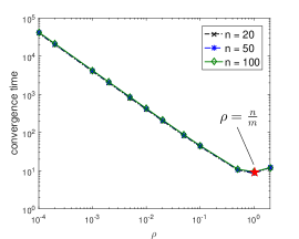
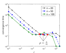
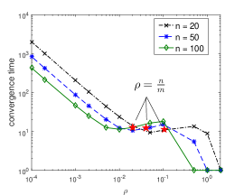
A direct approach is to apply similar techniques that accelerate the original ADMM. For example, reference [31] studies the optimal parameter selection of ρ𝜌\rho that maximizes the convergence rate δ𝛿\delta given in Theorem 1 and reference [35] uses preconditioning to improve the convergence rate. However, these approaches require the knowledge of the network structure, which might be unrealistic for large scale networks. Furthermore, the resulting parameter selection may not meet the consensus accuracy requirement and indeed does not provide the best practical performance. Here we propose a heuristic selection ρ=nm𝜌𝑛𝑚\rho=\frac{n}{m} which only requires (an estimate of) the number of nodes and the number of edges. Our intuition is based on the fact that a larger mn𝑚𝑛\frac{m}{n} indicates that an agent on the average has more neighboring information for its update. Therefore, a smaller ρ𝜌\rho provides adequate updates towards the consensus. Conversely, when agents have less information available, a larger ρ𝜌\rho can help accelerate the speed. The good performance of this selection is validated by simulations. When ρ=nm𝜌𝑛𝑚\rho=\frac{n}{m} fails to satisfy a given consensus accuracy constraint, a decreasing strategy can be used where the initial value of ρ𝜌\rho is set at nm𝑛𝑚\frac{n}{m} and decreases as the number of iterations increases. In the case where only n𝑛n is known but m𝑚m is not, the decreasing strategy may simply start with ρ=1𝜌1\rho=1.

IV-D Stopping Criterion

A natural approach for stopping BQ-CADMM is to set the maximum number of iterations at each node, which then requires characterization of the convergence time. While our current analysis does not have a closed-form result, we alternatively provide a rough upper bound based on our observations. At the beginning of the algorithm when local agent variables are far from the optima, i.e., when 𝒖k𝒖𝑮2superscriptsubscriptnormsuperscript𝒖𝑘superscript𝒖𝑮2\|\bm{u}^{k}-\bm{u}^{*}\|_{\bm{G}}^{2} is large, the CADMM update in (7) and (8) will make much progress towards the optima and the effect of the quantization operation 𝒬()𝒬\mathcal{Q}(\cdot) is negligible. Thus, BQ-CADMM and the original CADMM for the constrained least-squares problem have similar trajectories at early stages. When local variables becomes close to the optima, the original CADMM still has monotone decreasing 𝒖k𝒖𝑮2superscriptsubscriptnormsuperscript𝒖𝑘superscript𝒖𝑮2\|\bm{u}^{k}-\bm{u}^{*}\|_{\bm{G}}^{2} while BQ-CADMM either converges or cycles due to the quantization operation. This behavior is observed in all our simulations and an example is provided in Fig. 2. As such, a rough estimate can be obtained based on the convergence rate result of the original CADMM when applied to the constrained least-squares problem. Here we use the result from [36] where 𝒖k+1𝒖k𝑮2superscriptsubscriptnormsuperscript𝒖𝑘1superscript𝒖𝑘𝑮2\|\bm{u}^{k+1}-\bm{u}^{k}\|_{\bm{G}}^{2} is viewed as a metric of how close local variables are to the optima. The convergence rate of the original CADMM is

𝒖k+1𝒖k𝑮21k+1𝒖0𝒖𝑮2.superscriptsubscriptnormsuperscript𝒖𝑘1superscript𝒖𝑘𝑮21𝑘1superscriptsubscriptnormsuperscript𝒖0superscript𝒖𝑮2\displaystyle\hskip 2.0pt\|\bm{u}^{k+1}-\bm{u}^{k}\|_{\bm{G}}^{2}\leq\hskip 2.0pt\frac{1}{k+1}\|\bm{u}^{0}-\bm{u}^{*}\|_{\bm{G}}^{2}. (26)

We can bound the right-hand side of (26) by a small value and our simulations show that 4ρΔ24𝜌superscriptΔ24\rho\Delta^{2} is a good choice. Thus, a rough bound on convergence time, with xi0=αi0=0superscriptsubscript𝑥𝑖0superscriptsubscript𝛼𝑖00x_{i}^{0}=\alpha_{i}^{0}=0 for i=1,2,,n𝑖12𝑛i=1,2,\ldots,n, is given by

1Δ2(n𝒯𝒳(r¯)2+12ρ2λ2(𝑳)𝒓𝟏n𝒯𝒳(r¯)22).1superscriptΔ2𝑛subscript𝒯𝒳superscript¯𝑟212superscript𝜌2subscript𝜆2subscript𝑳superscriptsubscriptnorm𝒓subscript1𝑛subscript𝒯𝒳¯𝑟22\frac{1}{\Delta^{2}}\left(n\mathcal{T_{X}}(\bar{r})^{2}+\frac{1}{2\rho^{2}{\lambda_{2}(\bm{L}_{-})}}\|\bm{r}-\bm{1}_{n}\mathcal{T_{X}}(\bar{r})\|_{2}^{2}\right).

We remark that this rough bound is quite loose in most of our simulations; see Fig. 4. An upper bound on the convergence time, which depends on the network topology and agents’ data, may still be insufficient as these quantities are locally unknown. In fully distributed settings, we can run additional algorithms to determine if a consensus has been reached; see, e.g., [37, 38]. These additional algorithms may take a long running time in large networks and will require extra data communications. In general, finding a practically meaningful and efficient stopping criterion in a fully distributed manner remains open.

As to determining the cyclic behavior, nodes may record a certain number of consecutive variable values and check if any cycle exists. Though no bound on cyclic period is provided in this paper, our simulations show that the cyclic period is between 222 and 151515. In summary, we can set the maximum number of iterations or run the algorithm as long as permitted. If there is no convergence which can be determined by additional algorithms, we can then run other algorithms with agents’ data αik+risuperscriptsubscript𝛼𝑖𝑘subscript𝑟𝑖-\alpha_{i}^{k}+r_{i} which are bounded with a known bound at each node.

V Simulations

This section investigates the proposed algorithms via numerical examples. We construct a connected network with n𝑛n nodes and m𝑚m edges by first generating a complete graph of n𝑛n nodes and then randomly removing n(n1)2m𝑛𝑛12𝑚\frac{n(n-1)}{2}-m edges while ensuring the graph stays connected. Let Δ=1Δ1\Delta=1 throughout this section.

V-A Consensus Error

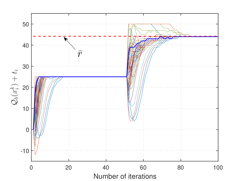
We first illustrate how BQ-CADMM and EBQ-CADMM proceed by showing the trajectories of agents’ variables. We simulate a connected network with n=50𝑛50n=50 nodes and m=100𝑚100m=100 edges. Let L=n2=25𝐿𝑛225L=\frac{n}{2}=25, ρ=nm=0.5𝜌𝑛𝑚0.5\rho=\frac{n}{m}=0.5, and ri𝒩(n,n2)similar-tosubscript𝑟𝑖𝒩𝑛superscript𝑛2r_{i}\sim\mathcal{N}(n,n^{2}). Set also the maximum iteration number of each BQ-CADMM to 505050. By this setting, it is very likely to have |r¯|>L¯𝑟𝐿|\bar{r}|>L and we thus apply EBQ-CADMM for data averaging. The trajectories of 𝒬b(xik)+ti,i=1,2,,nformulae-sequencesubscript𝒬𝑏superscriptsubscript𝑥𝑖𝑘subscript𝑡𝑖𝑖12𝑛\mathcal{Q}_{b}(x_{i}^{k})+t_{i},i=1,2,\ldots,n are plotted in Fig. 1. In this example, the desired average is 44.2044.2044.20 and the resulting consensus value of EBQ-CADMM is 444444. The consensus error is 0.200.200.20, which is much smaller than the error bound (1+4ρmn)Δ2=2.514𝜌𝑚𝑛Δ22.5(1+4\rho\frac{m}{n})\frac{\Delta}{2}=2.5. The figure also indicates that EBQ-CADMM calls BQ-CADMM twice with the first and second calls converging at iterations 171717 and 333333, respectively. As a note, we run this setup for 10,0001000010,000 times and no cyclic result is observed.
Refer to caption
Figure 1: Trajectories of EBQ-CADMM; n=50𝑛50n=50, m=100𝑚100m=100, L=n2𝐿𝑛2L=\frac{n}{2}, Δ=1Δ1\Delta=1, ρ=0.5𝜌0.5\rho=0.5, and ri(n,n2)similar-tosubscript𝑟𝑖𝑛superscript𝑛2r_{i}\sim\mathcal{(}n,n^{2}).

We next compare the proposed algorithms with DQ-CADMM that uses rounding quantizer 𝒬()𝒬\mathcal{Q}(\cdot) to investigate the effect of the bounded constraint. Denote 𝒕=[t1;t2;;tn]𝒕subscript𝑡1subscript𝑡2subscript𝑡𝑛\bm{t}=[t_{1};t_{2};\cdots;t_{n}] for EBQ-CADMM and define the iterative error as

{𝒬b(𝒙k)𝟏nr¯2/n,BQ-CADMM,𝒬b(𝒙k)+𝒕𝟏nr¯2/n,EBQ-CADMM,𝒬(𝒙k)𝟏nr¯2/n,DQ-CADMM,𝒙k𝟏nr¯/n,CADMM,casessubscriptnormsubscript𝒬𝑏superscript𝒙𝑘subscript1𝑛¯𝑟2𝑛BQ-CADMMsubscriptnormsubscript𝒬𝑏superscript𝒙𝑘𝒕subscript1𝑛¯𝑟2𝑛EBQ-CADMMsubscriptnorm𝒬superscript𝒙𝑘subscript1𝑛¯𝑟2𝑛DQ-CADMMnormsuperscript𝒙𝑘subscript1𝑛¯𝑟𝑛CADMM\displaystyle\begin{cases}{\left\|\mathcal{Q}_{b}({\bm{x}}^{k})-\bm{1}_{n}\bar{r}\right\|_{2}}/{\sqrt{n}},&~{}\text{BQ-CADMM},\\ {\left\|\mathcal{Q}_{b}({\bm{x}}^{k})+\bm{t}-\bm{1}_{n}\bar{r}\right\|_{2}}/{\sqrt{n}},&~{}\text{EBQ-CADMM},\\ {\left\|\mathcal{Q}({\bm{x}}^{k})-\bm{1}_{n}\bar{r}\right\|_{2}}/{\sqrt{n}},&~{}\text{DQ-CADMM},\\ {\left\|\bm{x}^{k}-\bm{1}_{n}\bar{r}\right\|/\sqrt{n}},&~{}\text{CADMM},\end{cases}

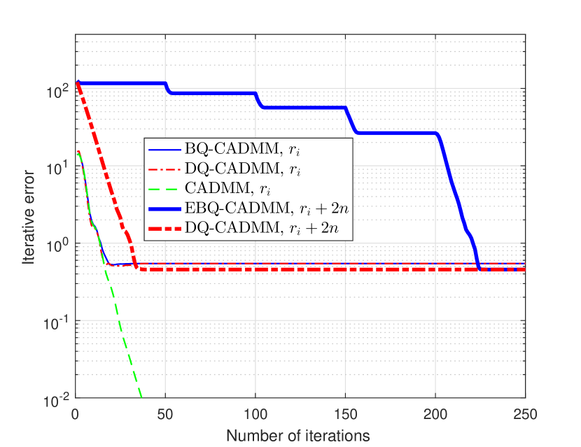
which is equal to the consensus error when a consensus is reached. Set n=75𝑛75n=75, m=200𝑚200m=200 and L=30𝐿30L=30. Pick ρ=0.5𝜌0.5\rho=0.5 and set the maximum iteration number of each BQ-CADMM call in EBQ-CADMM to 505050. We consider two cases: one with the average in the bounded set and the other with the average outside the set. Specifically, we generate ri𝒩(0,n2)similar-tosubscript𝑟𝑖𝒩0superscript𝑛2r_{i}\sim\mathcal{N}(0,n^{2}) and run the distributed averaging algorithms twice with data risubscript𝑟𝑖r_{i} and ri+2nsubscript𝑟𝑖2𝑛r_{i}+2n, respectively. We use BQ-CADMM for the former case since the average lies in the bounded set with high probability. Simulation result is presented in Fig. 2.
Refer to caption
Figure 2: Iterative errors of BQ-CADMM, EBQ-CADMM, DQ-CADMM, and CADMM; n=75𝑛75n=75, m=200𝑚200m=200, L=30𝐿30L=30, Δ=1Δ1\Delta=1, ρ=0.5𝜌0.5\rho=0.5, and ri𝒩(0,n2)similar-tosubscript𝑟𝑖𝒩0superscript𝑛2r_{i}\sim\mathcal{N}(0,n^{2}).

From Fig. 2, all quantized consensus algorithms converge to a consensus after certain iterations with consensus errors much smaller than the upper bound, computed to be 1.831.831.83. When r¯𝒳¯𝑟𝒳\bar{r}\in\mathcal{X}, BQ-CADMM and DQ-CADMM perform similarly and their iterative errors decrease exponentially until consensus is reached, while the original CADMM makes the iterative error decrease to 00. When |r¯|>L¯𝑟𝐿|\bar{r}|>L, DQ-CADMM converges much faster than EBQ-CADMM. This is because each BQ-CADMM call has iterations running even when a consensus is reached.

V-B Cyclic Period

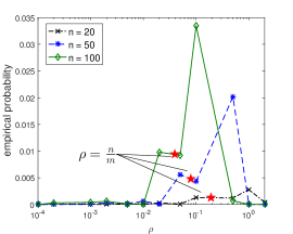
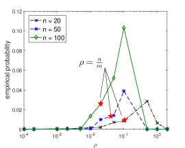
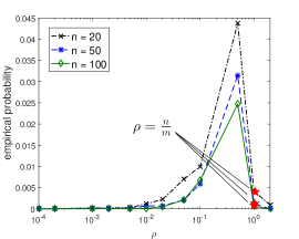
Since the convergent case can be viewed as the cyclic case with period T=1𝑇1T=1, we first investigate whether BQ-CADMM converges or cycles in various settings. Notice that the quantized consensus algorithm converges in all the above examples and indeed, BQ-CADMM and hence EBQ-CADMM tend to converge, particularly with small enough ρ𝜌\rho. To illustrate this, we simulate star graphs which have the smallest number of edges for a connected network, randomly generated connected graphs with intermediate numbers of edges, and complete graphs which have the highest number of edges. As Corollary 1 indicates that BQ-CADMM must converge when r¯¯𝑟\bar{r} is far from the bounded set 𝒳𝒳\mathcal{X}, we set L=30𝐿30L=30 and generate ri𝒩(0,100)+r0similar-tosubscript𝑟𝑖𝒩0100subscript𝑟0r_{i}\sim\mathcal{N}(0,100)+r_{0} where r0𝒩(0,25)similar-tosubscript𝑟0𝒩025r_{0}\sim\mathcal{N}(0,25) such that most simulated cases have r¯𝒳¯𝑟𝒳\bar{r}\in\mathcal{X}. We then run BQ-CADMM with different ρ𝜌\rho for the same data. The simulation result is plotted in Fig. 3, where each plotted value denotes the empirical probability of cyclic result in 10,0001000010,000 runs and both data and graph are randomly generated at each run.
Refer to caption
Refer to caption
Refer to caption
Figure 3: Empirical probability of cyclic case of BQ-CADMM in 10,0001000010,000 runs; ri𝒩(0,100)+r0similar-tosubscript𝑟𝑖𝒩0100subscript𝑟0r_{i}\sim\mathcal{N}(0,100)+r_{0} with r0𝒩(0,25)similar-tosubscript𝑟0𝒩025r_{0}\sim\mathcal{N}(0,25), L=30𝐿30L=30 and Δ=1Δ1\Delta=1. (a) star graph, (b) randomly generated graph with m=(n+2)(n1)4𝑚𝑛2𝑛14m=\left\lceil\frac{(n+2)(n-1)}{4}\right\rceil, (c) complete graph.

Fig. 3 indicates that BQ-CADMM always converges for large enough ρ𝜌\rho with which the consensus result has a large error bound, as discussed in Section IV-C. When ρ𝜌\rho decreases, the number of cyclic cases first increases and then decreases to 00. In particular, BQ-CADMM converges in all simulated examples with small enough ρ𝜌\rho. Another interesting observation is that peak occurrence of the cyclic case differs for different network structures. The star network has highest cyclic cases around ρ=0.5nm𝜌0.5𝑛𝑚\rho=0.5\frac{n}{m} and a larger network indicates less cyclic cases, while the intermediate and complete networks have cyclic cases centered around ρ=5nm𝜌5𝑛𝑚\rho=5\frac{n}{m} with larger networks having more cyclic cases.

In the same example, we also record the cyclic period when BQ-CADMM indeed cycles. We observe that the period of star networks is always 222 for all n𝑛n and ρ𝜌\rho, and the intermediate and complete networks have periods between 888 and 151515. While we cannot draw firm conclusions on cyclic period from the simulation result, we do find that the period in all cyclic cases consists of two consecutive quantization levels for each node, which can help derive better error bounds as discussed in Section IV-B.

V-C Convergence Time

To study how ρ𝜌\rho affects the convergence time of BQ-CADMM, we plot in Fig. 4 the average convergence time of the same example in the above section. We observe that BQ-CADMM converges immediately for large enough ρ𝜌\rho but again a large consensus error may exist. The convergence time is about 101010 when running BQ-CADMM with ρ=nm𝜌𝑛𝑚\rho=\frac{n}{m} for all network sizes and network structures. For small ρ𝜌\rho, the convergence time decreases polynomially as ρ𝜌\rho increases. The network structure also plays an important role here. For the star network, the convergence time is almost the same for all n𝑛n and a larger n𝑛n results in a slightly longer convergence time. On the other hand, the intermediate and complete networks have longer convergence time with smaller n𝑛n. Comparing the convergence time of the same network size, we also find that a denser network tends to converge faster for the same ρ𝜌\rho.

Refer to caption
Refer to caption
Refer to caption
Figure 4: Convergence time of BQ-CADMM where each plotted value is the average of 10,0001000010,000 runs; ri𝒩(0,100)+r0similar-tosubscript𝑟𝑖𝒩0100subscript𝑟0r_{i}\sim\mathcal{N}(0,100)+r_{0} with r0𝒩(0,25)similar-tosubscript𝑟0𝒩025r_{0}\sim\mathcal{N}(0,25), L=30𝐿30L=30 and Δ=1Δ1\Delta=1. (a) star graph, (b) randomly generated graph with m=(n+2)(n1)4𝑚𝑛2𝑛14m=\left\lceil\frac{(n+2)(n-1)}{4}\right\rceil, (c) complete graph.

V-D Parameter Selection

To achieve high consensus accuracy (e.g., the consensus error is within one quantization resolution), the consensus error bound of the cyclic case in Theorem 2 implies that one may need to pick a very small ρ𝜌\rho which can make BQ-CADMM slow to reach convergence or cycling. Fortunately, simulations indicate that BQ-CADMM converges in most cases and ρ𝜌\rho can be larger to meet the consensus error requirement in convergent cases. As such, we can start BQ-CADMM with a large ρ𝜌\rho for a number of iterations. Even though the local variables may not converge, they become close to the optima. We then pick a small ρ𝜌\rho and run BQ-CADMM with the current local variable values. We continue this process until either a convergence is reached and ρ𝜌\rho is such that the consensus error bound (11) meets the required consensus accuracy, or ρ𝜌\rho is small enough such that the cyclic error bound (13) satisfies the accuracy requirement. We suggest starting with ρ=nm𝜌𝑛𝑚\rho=\frac{n}{m} as it performs reasonably well in terms of both consensus accuracy and convergence time, as seen from Fig. 3 and Fig. 4. If only n𝑛n is known, we may simply start with ρ=1𝜌1\rho=1 as n1mn(n1)2𝑛1𝑚𝑛𝑛12n-1\leq m\leq\frac{n(n-1)}{2} for connected networks.

To further illustrate the strategy with decreasing step size, we next apply it to the same example in Section IV-B. Starting with ρ=nm𝜌𝑛𝑚\rho=\frac{n}{m}, we run BQ-CADMM for 505050 iterations if ρ>104𝜌superscript104\rho>10^{-4} and then reduce it by a factor of 101010. We repeat this process until ρ<104𝜌superscript104\rho<10^{-4} with which we run BQ-CADMM long enough such that either convergence or cycling is reached. The average convergence time of this strategy is presented in Table I. As one can see, this strategy reduces dramatically the convergence time. In addition, most iterations occur when ρ>104𝜌superscript104\rho>10^{-4} and BQ-CADMM only takes a few more iterations to reach the convergence result in all simulated cases when ρ104𝜌superscript104\rho\leq 10^{-4}.

TABLE I: Average convergence time of BQ-CADMM with and without using the decreasing strategy for parameter selection.
  Structure   Nodes Decreasing Parameter Fixed Parameter
Star 202020 251.2251.2251.2 3.97×1043.97superscript1043.97\times 10^{4}
505050 253.9253.9253.9 4.14×1044.14superscript1044.14\times 10^{4}
100100100 257.1257.1257.1 4.24×1044.24superscript1044.24\times 10^{4}
Intermediate 202020 203.9203.9203.9 5.13×1035.13superscript1035.13\times 10^{3}
5550 159.2159.2159.2 1.94×1031.94superscript1031.94\times 10^{3}
100100100 160.6160.6160.6 0.94×1030.94superscript1030.94\times 10^{3}
Complete 202020 203.3203.3203.3 2.00×1032.00superscript1032.00\times 10^{3}
505050 158.7158.7158.7 0.84×1030.84superscript1030.84\times 10^{3}
100100100 160.4160.4160.4 0.43×1030.43superscript1030.43\times 10^{3}

VI Conclusion and Discussion

This paper proposes BQ-CADMM and EBQ-CADMM for distributed average consensus using finite-bit bounded quantization. It is shown that BQ-CADMM is equivalent to applying rounding quantizer to the CADMM update of a constrained least-squares problem. Based on this fact, we establish that BQ-CADMM either converges or cycles within finite iterations and further derive the consensus error bounds by utilizing convexity properties. An advantage of our algorithm is that the agents’ data can be arbitrary; in contrast, existing quantized consensus algorithms that adopt finite-bit quantizers require the data to be bounded and a bound to be known. Noticing that the consensus error is large when the data average is much beyond the quantizer range, we proceed to develop EBQ-CADMM which is equivalent to repeated runs of BQ-CADMM. The resulting consensus error bound can be the same as that of using the unbounded rounding quantizer by picking a small enough algorithm parameter. Balancing fast convergence and small consensus error, an adaptive parameter selection scheme is devised that requires only the knowledge of the number of nodes.

While simulations show that BQ-CADMM converges fast in most cases, the current work lacks theoretical analysis (e.g., upper bound) on cyclic period and convergence time. A possible approach is to find a Lyapunov function with which one can characterize these two quantities under suitable assumptions. In addition, asynchronous protocols, link failures, and noisy communication channels can be studied under the BQ-CADMM framework.

Proof:

The proof is mainly based on the fact that |𝒬b(x~)|Lsubscript𝒬𝑏~𝑥𝐿|\mathcal{Q}_{b}(\tilde{x})|\leq L for any x~~𝑥\tilde{x}\in\mathbb{R}. We first prove the following:

𝒯𝒳(xik+1)={L,ifαik>(1+4ρ|𝒩i|)L+|ri|,L,ifαik<(1+4ρ|𝒩i|)L|ri|.subscript𝒯𝒳superscriptsubscript𝑥𝑖𝑘1cases𝐿ifsuperscriptsubscript𝛼𝑖𝑘14𝜌subscript𝒩𝑖𝐿subscript𝑟𝑖𝐿ifsuperscriptsubscript𝛼𝑖𝑘14𝜌subscript𝒩𝑖𝐿subscript𝑟𝑖\displaystyle\mathcal{T_{X}}(x_{i}^{k+1})=\begin{cases}-L,&{\text{if}}~{}\alpha_{i}^{k}>\left(1+4\rho|\mathcal{N}_{i}|\right)L+\left|r_{i}\right|,\\ L,&{\text{if}}~{}\alpha_{i}^{k}<-\left(1+4\rho|\mathcal{N}_{i}|\right)L-\left|r_{i}\right|.\\ \end{cases}

Assume that 𝒯𝒳(xik+1)>Lsubscript𝒯𝒳superscriptsubscript𝑥𝑖𝑘1𝐿\mathcal{T_{X}}(x_{i}^{k+1})>-L if αik>(1+4ρ|𝒩i|)L+|ri|superscriptsubscript𝛼𝑖𝑘14𝜌subscript𝒩𝑖𝐿subscript𝑟𝑖\alpha_{i}^{k}>\left(1+4\rho|\mathcal{N}_{i}|\right)L+\left|r_{i}\right|. Similar to (III-B), the xisubscript𝑥𝑖x_{i}-update of BQ-CADMM implies that 𝒯𝒳(xik+1)subscript𝒯𝒳superscriptsubscript𝑥𝑖𝑘1\mathcal{T_{X}}(x_{i}^{k+1}) minimizes a constrained least-squares function:

𝒯𝒳(xik+1)=subscript𝒯𝒳superscriptsubscript𝑥𝑖𝑘1absent\displaystyle\mathcal{T_{X}}(x_{i}^{k+1})= argminx~𝒳12(x~ri)2+ρ|𝒩i|x~2x~(ρ|𝒩i|𝒬b(xik)\displaystyle\hskip 2.0pt\operatorname*{arg\,min}_{\tilde{x}\in\mathcal{X}}\frac{1}{2}(\tilde{x}-r_{i})^{2}+\rho|\mathcal{N}_{i}|\tilde{x}^{2}-\tilde{x}\Bigg{(}\rho|\mathcal{N}_{i}|\mathcal{Q}_{b}({x_{i}^{k}})
+ρj𝒩i𝒬b(xjk)αik+ri)\displaystyle+\rho\sum_{j\in\mathcal{N}_{i}}\mathcal{Q}_{b}(x_{j}^{k})-\alpha_{i}^{k}+r_{i}\Bigg{)}
\displaystyle\triangleq argminx~𝒳Gik(x~)+αikx~,subscriptargmin~𝑥𝒳superscriptsubscript𝐺𝑖𝑘~𝑥superscriptsubscript𝛼𝑖𝑘~𝑥\displaystyle\hskip 2.0pt\operatorname*{arg\,min}_{\tilde{x}\in\mathcal{X}}G_{i}^{k}(\tilde{x})+\alpha_{i}^{k}\tilde{x},

where, for ease of presentation, we define

Gik(x~)superscriptsubscript𝐺𝑖𝑘~𝑥absent\displaystyle G_{i}^{k}(\tilde{x})\triangleq 12(x~ri)2+ρ|𝒩i|x~2x~(ρ|𝒩i|𝒬b(xik)\displaystyle\hskip 2.0pt\frac{1}{2}(\tilde{x}-r_{i})^{2}+\rho|\mathcal{N}_{i}|\tilde{x}^{2}-\tilde{x}\Bigg{(}\rho|\mathcal{N}_{i}|\mathcal{Q}_{b}({x_{i}^{k}})
+ρj𝒩i𝒬b(xjk)+ri).\displaystyle\hskip 2.0pt+\rho\sum_{j\in\mathcal{N}_{i}}\mathcal{Q}_{b}(x_{j}^{k})+r_{i}\Bigg{)}.

Since |𝒬b(x~)|Lsubscript𝒬𝑏~𝑥𝐿\left|\mathcal{Q}_{b}(\tilde{x})\right|\leq L for any x~~𝑥\tilde{x}\in\mathbb{R}, it is straightforward to verify that Gik(x~)superscriptsubscript𝐺𝑖𝑘~𝑥G_{i}^{k}(\tilde{x}) is Lipschitz continuous over 𝒳𝒳\mathcal{X}: for any x~,y~𝒳~𝑥~𝑦𝒳\tilde{x},\tilde{y}\in\mathcal{X},

|Gik(x~)Gik(y~)|<((1+4ρ|𝒩i|)L+|ri|)|x~y~|.superscriptsubscript𝐺𝑖𝑘~𝑥superscriptsubscript𝐺𝑖𝑘~𝑦14𝜌subscript𝒩𝑖𝐿subscript𝑟𝑖~𝑥~𝑦\displaystyle\left|G_{i}^{k}(\tilde{x})-G_{i}^{k}(\tilde{y})\right|<\left(\left(1+4\rho|\mathcal{N}_{i}|\right)L+\left|r_{i}\right|\right)\left|\tilde{x}-\tilde{y}\right|.

Now letting x~=L𝒳~𝑥𝐿𝒳\tilde{x}=-L\in\mathcal{X}, we have

Gik(x~)+αikx~(Gik(𝒯𝒳(xik+1))+αik𝒯𝒳(xik+1))superscriptsubscript𝐺𝑖𝑘~𝑥superscriptsubscript𝛼𝑖𝑘~𝑥superscriptsubscript𝐺𝑖𝑘subscript𝒯𝒳superscriptsubscript𝑥𝑖𝑘1superscriptsubscript𝛼𝑖𝑘subscript𝒯𝒳superscriptsubscript𝑥𝑖𝑘1\displaystyle\hskip 2.0ptG_{i}^{k}(\tilde{x})+\alpha_{i}^{k}\tilde{x}-\left(G_{i}^{k}\left(\mathcal{T_{X}}(x_{i}^{k+1})\right)+\alpha_{i}^{k}\mathcal{T_{X}}(x_{i}^{k+1})\right)
=\displaystyle= Gik(L)Gik(𝒯𝒳(xik+1))αikLαik𝒯𝒳(xik+1)superscriptsubscript𝐺𝑖𝑘𝐿superscriptsubscript𝐺𝑖𝑘subscript𝒯𝒳superscriptsubscript𝑥𝑖𝑘1superscriptsubscript𝛼𝑖𝑘𝐿superscriptsubscript𝛼𝑖𝑘subscript𝒯𝒳superscriptsubscript𝑥𝑖𝑘1\displaystyle\hskip 2.0ptG_{i}^{k}(-L)-G_{i}^{k}\left(\mathcal{T_{X}}(x_{i}^{k+1})\right)-\alpha_{i}^{k}L-\alpha_{i}^{k}\mathcal{T_{X}}(x_{i}^{k+1})
<\displaystyle< ((1+4ρ|𝒩i|)L+|ri|αik)(𝒯𝒳(xik+1)+L),14𝜌subscript𝒩𝑖𝐿subscript𝑟𝑖superscriptsubscript𝛼𝑖𝑘subscript𝒯𝒳superscriptsubscript𝑥𝑖𝑘1𝐿\displaystyle\hskip 2.0pt\left(\left(1+4\rho|\mathcal{N}_{i}|\right)L+\left|r_{i}\right|-\alpha_{i}^{k}\right)\left(\mathcal{T_{X}}(x_{i}^{k+1})+L\right),
<\displaystyle< 0,0\displaystyle\hskip 2.0pt0,

where the last inequality is because αik>(1+4ρ|𝒩i|)L+|ri|superscriptsubscript𝛼𝑖𝑘14𝜌subscript𝒩𝑖𝐿subscript𝑟𝑖\alpha_{i}^{k}>\left(1+4\rho|\mathcal{N}_{i}|\right)L+\left|r_{i}\right| and 𝒯𝒳(xik+1)>Lsubscript𝒯𝒳superscriptsubscript𝑥𝑖𝑘1𝐿\mathcal{T_{X}}(x_{i}^{k+1})>-L. This contradicts the fact that 𝒯𝒳(xik+1)subscript𝒯𝒳superscriptsubscript𝑥𝑖𝑘1\mathcal{T_{X}}(x_{i}^{k+1}) minimizes Gik(x~)+αikx~superscriptsubscript𝐺𝑖𝑘~𝑥superscriptsubscript𝛼𝑖𝑘~𝑥G_{i}^{k}(\tilde{x})+\alpha_{i}^{k}\tilde{x} over 𝒳𝒳\mathcal{X}. That 𝒯𝒳(xik+1)=Lsubscript𝒯𝒳superscriptsubscript𝑥𝑖𝑘1𝐿\mathcal{T_{X}}(x_{i}^{k+1})=L for αik<(1+4ρ|𝒩i|)L|ri|superscriptsubscript𝛼𝑖𝑘14𝜌subscript𝒩𝑖𝐿subscript𝑟𝑖\alpha_{i}^{k}<-\left(1+4\rho|\mathcal{N}_{i}|\right)L-\left|r_{i}\right| can be shown analogously.

If 𝒯𝒳(xik+1)=Lsubscript𝒯𝒳superscriptsubscript𝑥𝑖𝑘1𝐿\mathcal{T_{X}}(x_{i}^{k+1})=-L, the bounded quantization scheme implies 𝒬b(xik+1)=L𝒬b(xjk+1)subscript𝒬𝑏superscriptsubscript𝑥𝑖𝑘1𝐿subscript𝒬𝑏superscriptsubscript𝑥𝑗𝑘1\mathcal{Q}_{b}(x_{i}^{k+1})=-L\leq\mathcal{Q}_{b}(x_{j}^{k+1}) for any j𝒩i𝑗subscript𝒩𝑖j\in\mathcal{N}_{i}. Therefore, if αik>(1+4ρ|𝒩i|)L+|ri|superscriptsubscript𝛼𝑖𝑘14𝜌subscript𝒩𝑖𝐿subscript𝑟𝑖\alpha_{i}^{k}>(1+4\rho|\mathcal{N}_{i}|)L+|r_{i}|, we get

αik+1=αik+ρ|𝒩i|𝒬b(xik+1)ρj𝒩i𝒬b(xjk+1)αik.superscriptsubscript𝛼𝑖𝑘1superscriptsubscript𝛼𝑖𝑘𝜌subscript𝒩𝑖subscript𝒬𝑏superscriptsubscript𝑥𝑖𝑘1𝜌subscript𝑗subscript𝒩𝑖subscript𝒬𝑏superscriptsubscript𝑥𝑗𝑘1superscriptsubscript𝛼𝑖𝑘\displaystyle\alpha_{i}^{k+1}=\alpha_{i}^{k}+\rho|\mathcal{N}_{i}|\mathcal{Q}_{b}(x_{i}^{k+1})-\rho\sum_{j\in\mathcal{N}_{i}}\mathcal{Q}_{b}(x_{j}^{k+1})\leq\alpha_{i}^{k}.

Similarly, αik+1αiksuperscriptsubscript𝛼𝑖𝑘1superscriptsubscript𝛼𝑖𝑘\alpha_{i}^{k+1}\geq\alpha_{i}^{k} if αik<(1+4ρ|𝒩i|)L|ri|superscriptsubscript𝛼𝑖𝑘14𝜌subscript𝒩𝑖𝐿subscript𝑟𝑖\alpha_{i}^{k}<-(1+4\rho|\mathcal{N}_{i}|)L-|r_{i}|.

Next consider |αik|(1+4ρ|𝒩i|)L+|ri|superscriptsubscript𝛼𝑖𝑘14𝜌subscript𝒩𝑖𝐿subscript𝑟𝑖|\alpha_{i}^{k}|\leq(1+4\rho|\mathcal{N}_{i}|)L+|r_{i}|. In this case, we can simply use the triangle inequality to conclude that

|αik+1|superscriptsubscript𝛼𝑖𝑘1\displaystyle|\alpha_{i}^{k+1}| |αik|+ρ|𝒩i||𝒬b(xik+1)|+ρj𝒩i|𝒬b(xik+1)|absentsuperscriptsubscript𝛼𝑖𝑘𝜌subscript𝒩𝑖subscript𝒬𝑏superscriptsubscript𝑥𝑖𝑘1𝜌subscript𝑗subscript𝒩𝑖subscript𝒬𝑏superscriptsubscript𝑥𝑖𝑘1\displaystyle\leq|\alpha_{i}^{k}|+\rho|\mathcal{N}_{i}|\left|\mathcal{Q}_{b}(x_{i}^{k+1})\right|+\rho\sum_{j\in\mathcal{N}_{i}}\left|\mathcal{Q}_{b}(x_{i}^{k+1})\right|
(1+6ρ|𝒩i|)L+|ri|.absent16𝜌subscript𝒩𝑖𝐿subscript𝑟𝑖\displaystyle\leq(1+6\rho|\mathcal{N}_{i}|)L+|r_{i}|.

Since αi0=0superscriptsubscript𝛼𝑖00\alpha_{i}^{0}=0, we finally have |αik|(1+6ρ|𝒩i|)L+|ri|superscriptsubscript𝛼𝑖𝑘16𝜌subscript𝒩𝑖𝐿subscript𝑟𝑖|\alpha_{i}^{k}|\leq(1+6\rho|\mathcal{N}_{i}|)L+|r_{i}| for all k𝑘k. ∎

References

  • [1] S. Zhu and B. Chen, “Distributed average consensus with bounded quantization,” in Proc. IEEE Int. Workshop on Signal Process. Advances in Wireless Commun., Edinburgh, UK, Jul. 2016.
  • [2] J. N. Tsitsiklis, “Problems in decentralized decision making and computation,” DTIC Document, Tech. Rep., 1984.
  • [3] J. Tsitsiklis, D. Bertsekas, and M. Athans, “Distributed asynchronous deterministic and stochastic gradient optimization algorithms,” IEEE Trans. Autom. Control, vol. 31, no. 9, pp. 803–812, Sep. 1986.
  • [4] C. Xu and F. C. Lau, Load Balancing in Parallel Computers: Theory and Practice.   Dordrecht, Germany: Kluwer, 1997.
  • [5] W. Ren and R. W. Beard, “Consensus seeking in multiagent systems under dynamically changing interaction topologies,” IEEE Trans. Autom. Control, vol. 50, no. 5, pp. 655–661, May 2005.
  • [6] S. Boyd, A. Ghosh, B. Prabhakar, and D. Shah, “Randomized gossip algorithms,” IEEE Trans. Inf. Theory, vol. 52, no. 6, pp. 2508–2530, Jun. 2006.
  • [7] S. Kar, S. Aldosari, and J. M. F. Moura, “Topology for distributed inference on graphs,” IEEE Trans. Signal Process., vol. 56, no. 6, pp. 2609–2613, Jun. 2008.
  • [8] Y. Cao, W. Yu, W. Ren, and G. Chen, “An overview of recent progress in the study of distributed multi-agent coordination,” IEEE Trans. Ind. Inf., vol. 9, no. 1, pp. 427–438, Feb. 2013.
  • [9] L. Elsner, I. Koltracht, and M. Neumann, “On the convergence of asynchronous paracontractions with application to tomographic reconstruction from incomplete data,” Linear Algebra Appl., vol. 130, pp. 65–82, 1990.
  • [10] L. Xiao and S. Boyd, “Fast linear iterations for distributed averaging,” Syst. Contr. Lett., vol. 53, no. 1, pp. 65–78, 2004.
  • [11] A. Nedic, A. Olshevsky, A. Ozdaglar, and J. N. Tsitsiklis, “On distributed averaging algorithms and quantization effects,” IEEE Trans. Autom. Control, vol. 54, no. 11, pp. 2506–2517, Nov. 2009.
  • [12] T. C. Aysal, M. E. Yildiz, A. D. Sarwate, and A. Scaglione, “Broadcast gossip algorithms for consensus,” IEEE Trans. Signal Process., vol. 57, no. 7, pp. 2748–2761, Jul. 2009.
  • [13] I. D. Schizas, A. Ribeiro, and G. B. Giannakis, “Consensus in ad hoc WSNs with noisy links—Part I: Distributed estimation of deterministic signals,” IEEE Trans. Signal Process., vol. 56, no. 1, pp. 350–364, Jan. 2008.
  • [14] H. Zhu, G. B. Giannakis, and A. Cano, “Distributed in-network channel decoding,” IEEE Trans Signal Process, vol. 57, no. 10, pp. 3970–3983, Oct. 2009.
  • [15] T. Erseghe, D. Zennaro, E. Dall’Anese, and L. Vangelista, “Fast consensus by the alternating direction multipliers method,” IEEE Trans. Signal Process., vol. 59, no. 11, pp. 5523–5537, Nov. 2011.
  • [16] S. Boyd, N. Parikh, E. Chu, B. Peleato, and J. Eckstein, “Distributed optimization and statistical learning via the alternating direction method of multipliers,” Foundations and Trends in Machine Learning, vol. 3, no. 1, pp. 1–122, 2011.
  • [17] A. Kashyap, T. Başar, and R. Srikant, “Quantized consensus,” Automatica, vol. 43, no. 7, pp. 1192–1203, 2007.
  • [18] L. Schuchman, “Dither signals and their effect on quantization noise,” IEEE T. Commun. Techn., vol. 12, no. 4, pp. 162–165, Dec. 1964.
  • [19] T. C. Aysal, M. J. Coates, and M. G. Rabbat, “Distributed average consensus with dithered quantization,” IEEE Trans. Signal Process., vol. 56, no. 10, pp. 4905–4918, Oct. 2008.
  • [20] S. Zhu, Y. C. Soh, and L. Xie, “Distributed parameter estimation with quantized communication via running average,” IEEE Trans. Signal Process., vol. 63, no. 17, pp. 4634–4646, Sep. 2015.
  • [21] S. Kar and J. M. Moura, “Distributed consensus algorithms in sensor networks: quantized data and random link failures,” IEEE Trans. Signal Process., vol. 58, no. 3, pp. 1383–1400, 2010.
  • [22] R. Carli, F. Fagnani, P. Frasca, and S. Zampieri, “Gossip consensus algorithms via quantized communication,” Automatica, vol. 46, no. 1, pp. 70–80, 2010.
  • [23] S. Zhu and B. Chen, “Quantized cosensus by the ADMM: probabilistic versus deterministic quantizers,” IEEE Trans. Signal Process., vol. 64, no. 7, pp. 1700–1713, Apr. 2016.
  • [24] ——, “Corrections to ”quantized consensus by the ADMM: probabilistic versus deterministic quantizers”,” IEEE Trans. Signal Processing, vol. 65, no. 6, pp. 1638–1639, 2017.
  • [25] M. E. Chamie, J. Liu, and T. Başar, “Design and analysis of distributed averaging with quantized communication,” in Proc. 53rd IEEE Conf. Decision and Control, Los Angeles, CA, Dec. 2014.
  • [26] T. Li, M. Fu, L. Xie, and J. F. Zhang, “Distributed consensus with limited communication data rate,” IEEE Trans. Autom. Control, vol. 56, no. 2, pp. 279–292, Feb. 2011.
  • [27] S. Zhu and B. Chen, “Distributed detection over connected networks via one-bit quantizer,” in Proc. IEEE Int. Symp. Inf. Theory, Barcelona, Spain, Jul. 2016.
  • [28] ——, “Distributed detection in ad hoc networks through quantized consensus,” arXiv preprint arXiv 1612.01904, 2016.
  • [29] F. R. Chung, Spectral Graph Theory.   American Mathematical Soc., 1997, vol. 92.
  • [30] M. Fiedler, “Algebraic connectivity of graphs,” Czechoslovak Mathematical Journal, vol. 23, no. 2, pp. 298–305, 1973.
  • [31] W. Shi, Q. Ling, K. Yuan, G. Wu, and W. Yin, “On the linear convergence of the ADMM in decentralized consensus optimization,” IEEE Trans. Signal Process., vol. 62, no. 7, pp. 1750–1761, Apr. 2014.
  • [32] B. He and X. Yuan, “On the O(1/n)𝑂1𝑛O(1/n) convergence rate of the Douglas-Rachford alternating direction method,” SIAM J. Numer. Anal., vol. 50, no. 2, pp. 700–709, 2012.
  • [33] W. Deng and W. Yin, “On the global and linear convergence of the generalized alternating direction method of multipliers,” J. Sci. Comput., vol. 66, no. 3, pp. 889–916, 2016.
  • [34] S. Boyd and L. Vandenberghe, Convex Optimization.   Cambridge Univ. Press, 2004.
  • [35] P. Giselsson and S. Boyd, “Linear convergence and metric delection in Douglas-Rachford splitting and ADMM,” IEEE Trans. Autom. Control, to be published. doi:10.1109/TAC.2016.2564160.
  • [36] B. He and X. Yuan, “On non-ergodic convergence rate of douglas–rachford alternating direction method of multipliers,” Numerische Mathematik, vol. 130, no. 3, pp. 567–577, 2015.
  • [37] N. E. Manitara and C. N. Hadjicostis, “Distributed stopping for average consensus in undirected graphs via event-triggered strategies,” Automatica, vol. 70, pp. 121–127, 2016.
  • [38] V. Yadav and M. V. Salapaka, “Distributed protocol for determining when averaging consensus is reached,” in 45th Annual Allerton Conference on Communication, Control, and Computing, Monticello, IL, 2007.