An exploratory study of heavy domain wall fermions on the lattice

Abstract

We report on an exploratory study of domain wall fermions (DWF) as a lattice regularisation for heavy quarks. Within the framework of quenched QCD with the tree-level improved Symanzik gauge action we identify the DWF parameters which minimise discretisation effects. We find the corresponding effective 4$d$ overlap operator to be exponentially local, independent of the quark mass. We determine a maximum bare heavy quark mass of $am_{h}\approx 0.4$, below which the approximate chiral symmetry and O(a)-improvement of DWF are sustained. This threshold appears to be largely independent of the lattice spacing. Based on these findings, we carried out a detailed scaling study for the heavy-strange meson dispersion relation and decay constant on four ensembles with lattice spacings in the range $2.0-5.7\,\mathrm{GeV}$. We observe very mild $a^{2}$ scaling towards the continuum limit. Our findings establish a sound basis for heavy DWF in dynamical simulations of lattice QCD with relevance to Standard Model phenomenology.

1 Introduction

With LHCb and BESIII generating data, and Belle-II soon to start production, increasingly accurate Standard Model (SM) predictions for heavy flavour physics are dearly needed to constrain or hopefully identify new physics. These predictions typically involve matrix elements of the operators of the Weak Effective Hamiltonian among hadronic states. As a result they require a non-perturbative approach, making lattice QCD simulations crucial. This is why in the last few years several approaches to implement heavy quarks in simulations of lattice QCD have been proposed. Some of these are based on an effective description of the heavy degrees of freedom, such as the Non Relativistic treatment of the heavy quark (NRQCD) Lepage:1987gg ; Thacker:1990bm or Heavy Quark Effective Theory (HQET) Eichten:1989zv ; Heitger:2003nj , or on a non relativistic re-interpretation of relativistic discretisation ElKhadra:1996mp ; Christ:2006us ; Lin:2006ur ; Aoki:2001ra . More recently collaborations have started treating the charm and bottom quarks in the same relativistic framework used to discretise the light quarks, e.g. Follana:2006rc ; Blossier:2009hg . However, simulations of full lattice QCD where both the physical light quarks ($u$, $d$ and $s$) and the charm or heavier quarks are represented by the same discretisation are still rather scarce. The main reason is certainly that the relevant energy scales, associated with the pion and the heavy quark masses respectively, are computationally costly to reconcile. This is particularly true in a fully relativistic and dynamical setup with controlled finite volume and discretisation errors. Simulations in which all quarks are discretised in the same way have a number of advantages, though. For instance, continuum flavour symmetries at finite lattice spacing simplify many calculations. Moreover, only such a setup seems suitable for the study of GIM-cancellation, which is an important ingredient in a number of phenomenological applications Sachrajda:2015rea . This paper is the second Cho:2015ffa in a series towards a lattice phenomenology program with domain wall fermions (DWF) Kaplan:1992bt ; Shamir:1993zy , in particular Möbius DWF (MDWF) Brower:2004xi ; Brower:2005qw ; Brower:2012vk , as the discretisation for light as well as heavy quarks. Compared to Twisted Mass Frezzotti:2000nk , DWF offer the attractive properties of conserving both chiral and parity symmetries at finite lattice spacing. Compared to HISQ fermions Follana:2006rc , a single quark can be simulated without the need of taking the root of the determinant to eliminate the different tastes, thus providing a theoretically clean regularisation. Since we enter mostly uncharted territory with simulations of heavy DWF (see also Chen:2014hva ; Cho:2015ffa ; Lin:2006vc ), we dedicate this paper to the investigation of its basic properties. We are particularly interested in studying the approach of heavy-light meson observables to the continuum limit. Our simulations have been carried out within quenched QCD. This is computationally much cheaper than dynamical QCD and therefore allows us to access a much wider range of lattice spacings ($a^{-1}\approx 2.0-5.7$ GeV). While the quenched approximation is certainly not suited for making phenomenologically relevant predictions, we expect it to share a number of properties with the unquenched case. Most importantly, we expect that the continuum limit scaling observed in the quenched theory over a large range of lattice spacings will be qualitatively the same as in the dynamical theory. Such information is particularly valuable given that for phenomenologically relevant simulations only dynamical ensembles at coarser lattice spacings are currently available. The rest of the paper is organised as follows: in section 2 we outline the overall computational strategy followed in this paper, report on the properties of the generated quenched gauge field ensembles, define the quantities that we compute and discuss several more technical aspects of our computation. In section 3 we describe the tuning of the MDWF parameters. This is followed in section 4 by a study of the continuum limit scaling of the dispersion relation and decay constants. In section 5 we draw our conclusions. In the appendix we provide supplementary material, in particular the numerical values for all data underlying the analysis.

2 Computational strategy and setup

2.1 Strategy

The main purpose of this work is to gain a qualitative understanding of discretisation effects of heavy MDWF. To this end, we study the MDWF parameter space and the heavy quark mass dependence of basic heavy-heavy and heavy-strange meson matrix elements and the energy as the cutoff is varied. Simulations of the quenched theory allow us to adopt algorithms (over-relaxed Creutz:1987xi ; Kennedy:1985nu heat-bath Cabibbo:1982zn ) that are, compared to the algorithms used with dynamical quarks (Hybrid Monte Carlo Duane:1987de ), computationally much cheaper. To some extent the problem of critical slowing down DelDebbio:2004xh ; Schaefer:2010hu ; Flynn:2015uma can therefore be circumvented by brute force. This enables us to probe finer lattice spacings than those affordable in dynamical simulations and check the scaling of the theory towards the continuum limit in more detail. In order to reduce simulation costs further, a relatively small physical lattice volume of $L\approx 1.6$ fm was considered. The volume was kept approximately constant while decreasing the lattice spacing. Since the finite size effects in physical quantities are then constant across all simulated lattice spacings, cut-off effects can be studied in detail. An important point addressed in this study concerns the residual chiral symmetry breaking of MDWF. The restoration of chiral symmetry in the massless limit is crucial to the simulation of QCD on the lattice, and is also responsible for automatic $\mathcal{O}(a)$-improvement, which is especially important when studying heavy quark physics. In our notation, the five dimensional MDWF action is $S^{5}=\bar{\psi}D^{5}_{MDWF}\psi$, where

$$D^{5}_{MDWF} = \left(\begin{array}[]{cccccc}\tilde{D}&-P_{-}&0&\ldots&0&amP_{+}\\ -P_{+}&\ddots&\ddots&0&\ldots&0\\ 0&\ddots&\ddots&\ddots&0&\vdots\\ \vdots&0&\ddots&\ddots&\ddots&0\\ 0&\ldots&0&\ddots&\ddots&-P_{-}\\ amP_{-}&0&\ldots&0&-P_{+}&\tilde{D}\end{array}\right)\,,$$ (7)

and we define

$$D_{+}=(bD_{W}+1)\,,\;\;D_{-}=(1-cD_{W})\;\;{\rm and}\;\;\tilde{D}=(D_{-})^{-1}D_{+}\,,$$ (8)

with the usual chiral projectors $P_{\pm}=\frac{1}{2}(1\pm\gamma_{5})$ and the Wilson matrix $D_{W}(M)=M+4-\frac{1}{2}D_{\rm hop},$ where $D_{\rm hop}=(1-\gamma_{\mu})U_{\mu}(x)\delta_{x+\mu,y}+(1+\gamma_{\mu})U_{\mu}^{\dagger}(y)\delta_{x-\mu,y}$ acting in 4$d$. Besides the bare quark mass $am$, MDWF have two further input parameters that need to be specified in each simulation: the extent of the fifth dimension $L_{s}$ and the domain wall height parameter $M=-M_{5}$, respectively. More specifically, $M_{5}$ is the negative mass parameter in the 4-dimensional Wilson Dirac operator that resides in the 5-dimensional MDWF Dirac operator. Since both $L_{s}$ and $M_{5}$ are parameters of the discretisation rather than of QCD we have some freedom in varying them. In the limit $L_{s}\to\infty$ and with the Wilson kernel this formalism coincides with the overlap formulation Neuberger:1997bg ; Neuberger:1997fp and allows for the simulation of a four-dimensional chirally symmetric theory (in the limit of massless quarks) that is free of doublers. When $L_{s}$ is finite however, chiral symmetry remains broken by a small amount. This can be quantified by measuring the amount of additive quark mass renormalisation, also known as residual mass $m_{\mathrm{res}}$ (defined later in 2.3). For a given extent of the fifth dimension, the parameter $M_{5}$ sets the scale for the exponential localisation of the chiral modes of the fermionic fields at the boundaries of the 5th dimension. The decay rate of the physical mode away from the boundary is however also modified by the presence of an explicit quark mass term, and care must be taken in order to maintain the localisation of the physical modes on the boundary Kaplan:1992bt ; Jansen:1992tw ; Kaplan:2009yg ; Christ:2004gc ; Lin:2006vc ; Liu:2003kp . As we will see, this becomes particularly crucial for heavy input quark masses. We will study how the choice of a heavy quark mass $am=am_{h}$ and $M_{5}$ changes the ultra-violet properties of the discretisation. In the following we chose an extent $L_{s}=12$ of the fifth dimension, which guarantees a small value of $m_{\rm res}$ for light quarks Blum:2014tka . The particular choice of MDWF is the same implementation as the one used in Blum:2014tka with a Möbius scale of $\alpha=b+c=2$.

2.2 Ensemble generation

We generated ensembles based on the tree-level Symanzik improved Curci1983a ; Luscher:1984xn gauge action with lattice spacings in the range of 0.034–0.1 fm. The gauge configurations have been produced with the heat-bath algorithm Cabibbo:1982zn ; Creutz:1987xi ; Kennedy:1985nu . The coarser three ensembles were generated using CHROMA Edwards:2004sx , whereas for the finest lattice spacing (which involved the highest computational cost) we recurred to a faster implementation, especially optimised for IBM BG/Q Sanfilippo_code . In tables 1, 2 and 3 we summarise the simulation parameters used and basic ensemble properties.

$\beta$	$L/a$	$N_{\mathrm{sweeps}}$
4.41	16	10 k
4.66	24	20 k
4.89	32	600 k
5.20	48	1.4 M

Table 1: Coupling constant $\beta$, volume in lattice units ($N_{x}=N_{y}=N_{z}=L/a$, $N_{t}=2L/a$), and number of update sweeps ($N_{\mathrm{sweeps}}$) after thermalisation. Each sweep consists of 1 heat-bath combined with 8 over-relaxation steps.

Lattice spacings have been determined at each simulated $\beta$ by enforcing the Wilson-flow scale $w_{0}$ Luscher:2010iy ; Borsanyi:2012zs to take its “physical” value, which we assumed to be $w_{0}^{\mathrm{phys}}=0.17245(99)\,\mathrm{fm}$ as recently determined in Blum:2014tka . We kept the physical volume fixed such that the spatial extent remained at about $1.6\,{\rm fm}$ (cf. table 2).

$\beta$	Plaquette	$w_{0}/a$	$a^{-1}[\mathrm{GeV}]$	$L[\mathrm{fm}]$
4.41	0.62637(3)	1.767(3)	2.037(08)	1.550(6)
4.66	0.651421(12)	2.499(8)	2.861(09)	1.655(5)
4.89	0.671257(5)	3.374(11)	3.864(12)	1.634(5)
5.20	0.694149(4)	5.007(28)	5.740(22)	1.650(6)

Table 2: Plaquette value, lattice spacing ($a^{-1}$) and spatial extent ($L$) resulting from the comparison of $w_{0}/a$ with the physical value quoted in the text. Errors on dimensional quantities include the systematic uncertainties arising from the physical value of $w_{0}$.

The evolution of the topological charge $Q$ (measured with the GLU package Hudspith_code ) is illustrated in figure 8 in appendix A. These quantities are expected to couple strongly to the slowest evolving mode in the evolution of the algorithm Schaefer:2010hu . We obtain sets of decorrelated measurements by choosing only configurations for further processing that are separated by $N_{\mathrm{sep}}$ intermittent update steps with $N_{\mathrm{sep}}$ larger than twice its autocorrelation time $\tau_{int}\left(Q^{2}\right)$ Wolff:2003sm , as detailed in table 3.

$\beta$	$\tau_{int}\left(Q_{\textrm{top}}\right)$	$\tau_{int}\left(Q_{\textrm{top}}^{2}\right)$	$N_{\textrm{sep}}$	$N_{{\rm cnfg}}$
$4.41$	$15(3)$	$10.5(1.6)$	$100$	$100$
$4.66$	$160(60)$	$74(22)$	$200$	$100$
$4.89$	$200(100)$	$170\left(80\right)$	$500$	$111$
$5.20$	$28000\left(13000\right)$	$12000\left(4000\right)$	$40000$	$36$

Table 3: Autocorrelation time of topological charge ($\tau_{int}\left(Q_{\textrm{top}}\right)$) and of charge squared ($\tau_{int}\left(Q_{\textrm{top}}^{2}\right)$) in units of sweep steps; number of sweeps separating each configuration included in the measured ensemble ($N_{\mathrm{sep}}$), and total number of gauge configurations considered.

2.3 Observables

The pseudoscalar decay constant $f_{X}$ is defined as the matrix element of the conserved MDWF axial vector current Boyle:2014hxa between a pseudoscalar meson state $X$ and the vacuum,

$$\left\langle 0\right|\mathcal{A}_{0}\left|X\left(\mathbf{p}\right)\right\rangle=E_{X}(\mathbf{p})f_{X}\,.$$ (9)

We determine the decay constant $f_{X}$ and the energy $E_{X}(\mathbf{p})$ of the pseudoscalar state $X$ from fits to the time dependence of Euclidean QCD two-point correlation functions projected onto momentum $\mathbf{p}$,

$$C_{MN}^{s_{1},s_{2}}(t)\equiv\sum_{\mathbf{x},\mathbf{y}}e^{i\mathbf{p}(\mathbf{x}-\mathbf{y})}\langle\,O^{s_{1}}_{M}(t,\mathbf{y})\,\left(O^{s_{1}}_{N}(0,\mathbf{x})\right)^{\dagger}\,\rangle\stackrel{{\scriptstyle{\rm large}\,t}}{{=}}\frac{Z^{s_{2}}_{M}(\mathbf{p})\left(Z^{s_{1}}_{N}(\mathbf{p})\right)^{\ast}}{2E(\mathbf{p})}\left(e^{-E(\mathbf{p})t}\pm e^{-E(\mathbf{p})(T-t)}\right)\,.$$ (10)

The operator $O^{s_{i}}_{M}$ is an interpolating operator with the quantum numbers of the meson, i.e. $O^{s}_{M}=\bar{q}_{2}\,\omega_{s}\,\Gamma_{M}q_{1}$ , where we consider the pseudoscalar case $\Gamma_{P}=\gamma_{5}$ and the axial vector case $\Gamma_{A}=\gamma_{0}\gamma_{5}$, respectively. The superscript $s$ indicates the smearing type induced via the spacial smearing kernel $\omega$, which in the simulations presented here is either local ($s=L$, $\omega(\mathbf{x},\mathbf{y})=\delta_{\mathbf{x},\mathbf{y}}$) or Gaussian via Jacobi iteration Gusken:1989ad ; Alexandrou:1990dq ; Allton:1993wc (see table 4 for our choice of smearing radii). The constants $Z^{s_{i}}_{M}$ are defined by $Z^{s_{i}}_{M}=\langle X(\mathbf{p})\,|\,\left(O^{s_{i}}_{M}\right)^{\dagger}\,|\,0\,\rangle$ where $X$ is the corresponding meson state. The fits leading to the extraction of masses and decay constants are multi-channel fits to combinations of the two-point correlation functions $C_{AA}$, $C_{AP}$, $C_{PA}$ and $C_{PP}$. We note the relation between the conserved MDWF axial current Boyle:2014hxa ; Blum:2014tka and the renormalised local axial current $\mathcal{A}_{0}=\mathcal{Z_{A}}A_{0}$, where $\mathcal{Z_{A}}$ is the axial vector current renormalisation constant. A further quantity that we wish to monitor during our simulations is the residual quark mass $am_{\rm res}$ Boyle:2014hxa , which provides an estimate of residual chiral symmetry breaking in the MDWF formalism. It is defined in terms of the axial Ward identity (AWI)

$$a\Delta^{-}_{\mu}\langle(\bar{\psi}\gamma_{5}\psi)(x)|{\cal A}_{\mu}(y)\rangle=\langle(\bar{\psi}\gamma_{5}\psi)(x)|2amP(y)+2J_{5q}(y)\rangle\,,$$ (11)

where $\Delta_{\mu}^{-}$ is the lattice backward derivative and $am$ is the bare quark mass in lattice units in the Lagrangian. It motivates the definition

$$am_{\rm res}=\frac{\sum\limits_{\mathbf{x}}\langle J_{5q}(x)P(0)\rangle}{\sum\limits_{\mathbf{x}}\langle P(x)P(0)\rangle}\,.$$ (12)

Here, $J_{5q}$ is the pseudoscalar density in the centre of the 5th dimension. We compute the correlation functions in eq. (10) with two types of quark sources. The analysis of the decay constant and the residual mass is based on $\mathbb{Z}_{2}$ noise sources and the one-end-trick Foster:1998vw ; McNeile:2006bz ; Boyle:2008rh (in this case we only consider $\mathbf{p}=\mathbf{0}$) while the analysis of the dispersion relation is based on point source data. The computation of heavy quark propagators by means of conjugate gradient type algorithms can be affected by round-off errors Juttner:2005ks . We monitor proper convergence during the computation of the quark propagators by checking that the desired solver residual is fulfilled on all time slices using the time slice residual Juttner:2005ks defined as

$$r_{t}={\rm Max}_{t}\frac{\left|D\psi-\eta\right|_{t}}{\left|\psi\right|_{t}}\,,$$ (13)

where $\left|x\right|_{t}$ is the norm of the vector $x$ restricted to time slice $t$. We determined statistical errors using the bootstrap method with 500 samples.

$\beta$	$L/a$	$r_{sm}^{\mathrm{P}}$	$r_{sm}^{\mathbb{Z}_{2}}$	$am_{s}^{\mathrm{phys}}$	$am_{h}$
					start	step	stop
4.41	16	2.8	4.5	0.03455(63)	0.1	0.05	0.4
4.66	24	4.0	6.0	0.02416(36)	0.066	0.033	0.396
4.89	32	8.8	7.5	0.01805(33)	0.07	0.04	0.39
5.20	48	11.7	11.7	0.01145(31)	0.04	0.04	0.28

Table 4: Simulated strange and heavy input quark masses $am_{h}$ and the choices of smearing radii for heavy quark masses. The simulated bare quark masses are quoted in lattice units for the MDWF action. The heavy quark masses starting from “start” with a step of “step” and ending at “end” are simulated. $r_{sm}^{\mathrm{P}}$ and $r_{sm}^{\mathbb{Z}_{2}}$ refer to the choice of the smearing parameter for the Gaussian smearing of the source/sink of the propagators for the point and $\mathbb{Z}_{2}$ noise sources, respectively. For the Gaussian smearing we employed 400 Jacobi iterations. All measurements are carried out with MDWF with parameters $L_{s}=12$.

3 Tuning MDWF for charm

In this section we present results for the $am_{h}$ and $M_{5}$ dependence of the heavy-heavy meson decay constant $f_{hh}$ and the residual mass $am_{\rm res}$.

3.1 $M_{5}$ dependence

The left hand panel of figure 1 shows the dependence of the heavy-heavy decay constant on the heavy-heavy inverse pseudoscalar mass $m_{hh}$ observed on the coarsest ($\beta=4.41$) ensemble. We normalise the results for a given $M_{5}$ by the value of the decay constant at $m_{hh}=1.5$ GeV as obtained from a polynomial interpolation. For small values of $m_{hh}$ the decay constant shows little dependence on the value of $M_{5}$, but as $m_{hh}$ is increased a strong dependence is observed. The right hand panel of figure 1 shows the same data for $M_{5}=1.4,\,1.6$ and 1.8 together with the corresponding results on the finer $\beta=4.66$ ensemble. For $M_{5}=1.6$ the results from the $\beta=4.41$ and $\beta=4.66$ align almost perfectly. This provides a first indication that for this choice of $M_{5}$ cutoff effects are small. Other choices of $M_{5}$ would offer viable alternatives but with more pronounced cutoff effects.

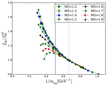
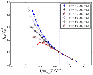
Figure 1: Left: decay constant $f_{hh}$ for heavy-heavy pseudoscalar mesons as a function of the inverse pseudoscalar mass $m_{hh}$, for different values of $M_{5}$ on the coarsest ensemble. The data is normalised at $m_{hh}^{\mathrm{norm}}=1.5\mathrm{\,GeV}$ to remove the multiplicative renormalisation constant. The vertical lines correspond to $m_{\eta_{c}}$ and to $m_{hh}^{norm}$. Right: overlay of the results obtained at two different lattice spacings for three values of $M_{5}$.

3.2 Residual mass

Next we quantify how the residual chiral symmetry breaking is affected by $M_{5}$ by observing the response of the size of the residual mass to variations in $am_{h}$ and $M_{5}$. In the left panel of figure 2 we show the ratio of correlation functions eq. (12) from which we determine $am_{\rm res}$ as a function of time for several values of the quark mass at $M_{5}=1.6$. Note that for large $t$ the time dependence in ratio eq. (12) is expected to cancel between the numerator and denominator. While the expected (constant) behaviour in time is observed for small quark masses, this is strikingly not the case for values of $am_{h}^{bare}\gtrsim 0.4$. In these cases it is difficult to interpret the operator $J_{5q}$’s matrix element as a constant, residual additive mass correction in the chiral Ward identity. The effect is of course rather small compared to the explicit chiral symmetry breaking, but there is a risk that the physical modes no longer remain bound to the walls of the fifth dimension in this large mass limit. To be more quantitative, we define $am_{\mathrm{res}}(t=T/2)$ as the value of this correlator ratio in the (temporal) middle of the lattice. Note, however, that above $am_{h}\approx 0.4$ the meaning of $am_{\rm res}$ as a unique measure of residual chiral symmetry breaking is no longer clear, only indicative. The right hand panel in figure 2 shows $am_{\rm res}(t=T/2)$ as a function of the quark mass. We observe the same qualitative behaviour for all values of $M_{5}$: as the input quark mass is increased beyond $am_{h}\approx 0.4$ the residual mass $am_{\rm res}(t=T/2)$ starts to increase drastically. Although this quantity is $L_{s}$ dependent, it is likely unsafe to use domain wall fermions at masses where the physical modes become unbound from the walls and the matrix elements of $J_{5q}$ have such non-trivial behaviour. The impact on 4$d$ observables will be studied later in this paper.

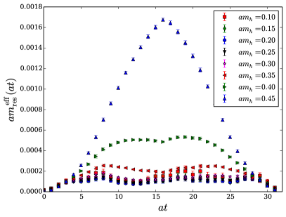
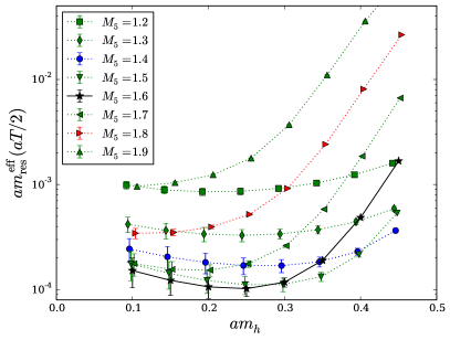
Figure 2: Left: behaviour of the effective residual mass $am_{\mathrm{res}}^{\mathrm{eff}}$ as a function of time on our coarsest ensemble, for $M_{5}=1.6$. Right: residual mass determined at $t=T/2$ as a function of the bare quark mass for several values of $M_{5}$.

3.3 Locality of the effective 4$d$ Dirac operator

Given the above observation indicating the reduced binding of surface states of MDWF above $am_{h}\approx 0.4$, a further concern one might have is that we should check the locality property of the corresponding effective 4$d$ MDWF Dirac operator. The connection of the 5$d$ MDWF operator $D^{5}_{MDWF}$ defined in eq. (7) to a four dimensional effective theory is well established in the literature, Borici:1999zw ; Borici:1999da ; Brower:2004xi ; Brower:2005qw ; Brower:2012vk ; Kennedy:2006ax ; Blum:2014tka . We identify $D_{ov}$ as an approximation to the overlap operator with approximate sign function

$$\epsilon(H_{M})=\frac{(1+H_{M})^{L_{s}}-(1-H_{M})^{L_{s}}}{(1+H_{M})^{L_{s}}+(1-H_{M})^{L_{s}}}\,,$$ (14)

where the Möbius kernel is

$$H_{M}=\gamma_{5}\frac{(b+c)D_{W}}{2+(b-c)D_{W}}\,.$$ (15)

The transfer matrix in the fifth dimension can be identified as

$$\begin{array}[]{ccc}T^{-1}=-[H_{M}-1]^{-1}[H_{M}+1].\end{array}$$ (16)

The effective overlap operator may be simply found as

$$D_{ov} = \left[{\cal P}^{-1}D^{5}_{MDWF}(am=1)^{-1}D^{5}_{MDWF}(am){\cal P}\right]_{11}\,$$ (17)

$$= \left[\frac{1+am}{2}+\frac{1-am}{2}\gamma_{5}\frac{T^{-L_{s}}-1}{T^{-L_{s}}+1}\right],$$ (18)

where this is known to reduce to the standard overlap formalism in the limit $L_{s}\to\infty$ and when $b=c$, and the projection matrix ${\cal P}$ is

$${\cal P} = \left(\begin{array}[]{ccccc}P_{-}&P_{+}&0&\ldots&0\\ 0&\ddots&\ddots&0&\vdots\\ \vdots&0&\ddots&\ddots&0\\ 0&\ldots&0&\ddots&P_{+}\\ P_{+}&0&\ldots&0&P_{-}\end{array}\right).$$ (24)

Following eq. (18), we may place the mass dependence of $D_{ov}(am)$ at non zero mass in the following form:

$$D_{ov}(am) = \left[\frac{1+am}{2}+\frac{1-am}{2}\gamma_{5}\frac{T^{-L_{s}}-1}{T^{-L_{s}}+1}\right]$$ (25)

$$= am+(1-am)D_{ov}(0)$$ (26)

$$= (1-am)\left[\frac{am}{1-am}+D_{ov}(0)\right].$$ (27)

We see that the kinetic term in the four dimensional effective action should remain unaltered as the mass is changed up to a trivial rescaling factor $(1-am)$ affecting the surface field renormalisation. The induced overlap bare mass is therefore better interpreted as the combination $\frac{am}{1-am}$, which of course varies non-linearly and diverges as we take the domain wall mass towards the Pauli-Villars mass of unity. The exponential locality Hernandez:1998et is fully encoded in the massless operator, and is independent of the quark mass. So, from this perspective there should be no locality issues as we take the mass large, since the kinetic term is trivially rescaled compared to the light mass case. We demonstrate this with a second use of eq. (18). The effective operator may be constructed by the simple application of the inverse of the Pauli Villars operator. Following the methodology of ref. Hernandez:1998et we now study the locality properties of this operator. We start by defining a point source $\xi$,

$$\xi_{\alpha,a}\left(x\right)=\begin{cases}1&x=y,\ \alpha=a=0\,({\rm spin,colour})\\ 0&{\rm otherwise},\end{cases}$$ (28)

where $y$ is the source location, and $\psi$ is the result of the multiplication of the effective 4$d$ Dirac operator with $\xi$,

$$\psi=D_{ov}\xi\,.$$ (29)

We say $D_{ov}$ is strictly local (or “ultralocal”) if the only non-zero contributions to $\left(D_{ov}\xi\right)\left(x\right)$ come from a finite set of terms $D_{ov}\left(x,y\right)\xi\left(y\right)$ with $y$ in the vicinity of $x$ Hernandez:1998et . We collect all lattice points $\left\{x\right\}_{r}$ separated by $r$ hoppings from the origin, such that $x\in\left\{x\right\}_{r}$ if $\left|x\right|_{1}=r$. Here $\left|x\right|_{1}$ is the “taxi driver” (or “Manhattan”) norm of $x$, defined by

$$\left|x\right|_{1}=\sum_{\mu}\min\left\{\left|x_{\mu}\right|,\,\left|N_{\mu}-x_{\mu}\right|\right\}\,,$$ (30)

where $N_{\mu}$ is the number of lattice sites along the $\mu$ axis. This definition accounts for the periodicity of the lattice. Finally, for each value of $r$ we define the maximum of the norm of $\psi$ at the set of points $\left\{x\right\}_{r}$:

$$f\left(r\right)=\max\left\{\left|\psi\left(x\right)\right|\forall\,x\in\left\{x\right\}_{r}\right\}\,.$$ (31)

In the following we will study $f\left(r\right)$ for values of the bare heavy quark mass in lattice units of $am_{h}=0.1$ and $am_{h}=0.5$ with $M_{5}=1.6$ on our $\beta=4.41$, $\beta=4.66$ and $\beta=4.89$ ensembles. In figure 3 we show the function $f\left(r\right)$ for two bare quark masses on all three ensembles. As expected, we observe that the slope of $f\left(r\right)$ is independent of the bare quark mass as well as of the lattice spacing, indicating that locality is recovered in the continuum limit. We can make a more quantitative statement for the mass independence of the locality of $D_{ov}(am)$: motivated by eq. (26) we define the function $\tilde{f}$:

$$\tilde{f}_{m}\left(r\right)=\max\left\{\left|\psi\left(x\right)-am\,\xi(x)\right|\forall\,x\in\left\{x\right\}_{r}\right\}\,,$$ (32)

where we have introduced a term to subtract the additive mass term in eq. (26). We can then define the ratio

$$R(r)=\frac{\tilde{f}_{m_{1}}(r)(1-am_{2})}{\tilde{f}_{m_{2}}(r)(1-am_{1})}\,,$$ (33)

where the subscripts indicate the bare quark masses at which the function $f$ was evaluated ($am_{1}=0.1$ and $am_{2}=0.5$). According to eq. (26), we expect $R(r)=1$, which is confirmed by our data to the level of arithmetic precision used in the computation. This provides a strong consistency check of our setup and our understanding of the locality of the MDWF operator.

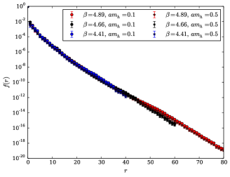
Figure 3: Localisation function (with logarithmic y-scale) for the effective MDWF operator at two bare quark masses on the three coarser quenched ensembles.

4 Continuum limit of the decay constant and the dispersion relation

The results in the previous section provide the first evidence for a region in parameter space where MDWF can be used as a suitable discretisation for heavy quarks. To further substantiate this picture we now fix $M_{5}=1.6$ and study the continuum scaling of a basic heavy-strange pseudoscalar meson matrix element, the decay constant, and the corresponding dispersion relation, as a function of the mass of the heavy quark.

4.1 Choice of strange and heavy quark masses

We study the continuum limit along lines of constant strange and heavy quark mass. We fix the $s$-quark by considering a fictitious meson $\eta_{s}$ composed of two different quarks, $s$ and $s^{\prime}$, of degenerate mass $m_{s}$. This meson differs from the physical $\eta-\eta^{\prime}$ mesons by quark-disconnected Wick contractions. We tuned the strange quark mass to its “physical value”, by imposing at each lattice spacing the mass of the simulated $\eta_{s}$ meson to reproduce $m_{\eta_{s}}=0.6858(40)\,\mathrm{GeV}$ Davies:2010ip . This sets a common renormalised strange quark mass on all the ensembles. In table 4 we report on the values of the corresponding bare strange quark mass and on our choices for the simulated heavy quark masses.

4.2 Decay constants for heavy-strange mesons

We consider the renormalised ratio

$$R_{sh}=\frac{f_{sh}\sqrt{m_{sh}}}{f_{sh}^{norm}\sqrt{m_{sh}^{norm}}}\,,$$ (34)

where we introduce $f_{sh}^{norm}\sqrt{m_{sh}^{norm}}$, interpolated to $m_{sh}=1$ GeV, to cancel the axial current renormalisation constant. We also include in both the numerator and denominator a factor of $\sqrt{m_{sh}}$ to make both of these quantities individually finite in the limit $am_{h}\to\infty$. We interpolate $R_{sh}$ to the reference pseudoscalar masses 1.3, 1.6, $m_{D_{s}}=1.9685$ Agashe:2014kda and 2.4 GeV on all ensembles. To fulfil the constraint $am_{h}\leq 0.4$ we are forced to drop the coarsest lattice spacing for the heaviest mass considered. A first visual inspection (see figure 4) suggests the absence of cutoff effects beyond $O(a^{2})$. Moreover, cutoff effects are observed to be very mild for the choice $M_{5}=1.6$, in agreement with the observation made in section 3. To obtain a more quantitative understanding we perform continuum limit extrapolations by considering two different fit ansätze, namely

$$R_{1}\left(a\right) \equiv R_{a=0}+D_{2}a^{2}\,,$$

$$R_{2}\left(a\right) \equiv R_{a=0}+E_{2}a^{2}+E_{4}a^{4}\,.$$ (35)

The results are illustrated in figure 4 as solid and dashed lines with error bands, respectively, and the resulting fit coefficients are listed in table 5.

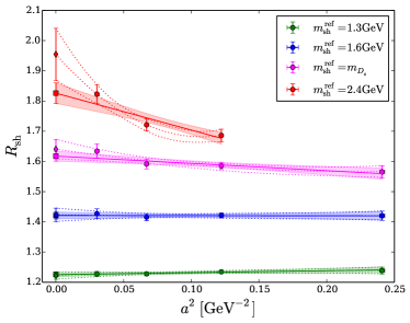
Figure 4: Continuum limit of the ratio of heavy-strange decay constants at different reference pseudoscalar masses with linear (dashed shaded error band, square-symbols) and quadratic (dotted lines, diamond symbols) polynomials in $a^{2}$.

For the two lightest reference masses, 1.3 and 1.6 GeV, the slope of the continuum limit is compatible with zero. For higher masses the continuum limit starts exhibiting a significant slope. In fact, the dimensionless term $D_{2}a^{2}/R\left(a=0\right)$, which indicates the fractional amount of discretisation errors, is around 2% for the physical $D_{s}$ meson on the coarsest ensemble ($a^{-1}\approx 2$ GeV), and of $\mathcal{O}\left(1\%\right)$ on the next finest one ($a^{-1}\approx 2.9$ GeV). At the level of statistical precision achieved here the fits reveal only a very mild sensitivity to higher order ($O(a^{4})$) coefficients: $E_{4}$ is compatible with zero within one standard deviation.

$m_{sh}^{\mathrm{ref}}[\mathrm{GeV}]$	$R_{a=0}$	$D_{2}[\mathrm{GeV}^{2}]$	$\chi^{2}/\mathrm{dof}$	$p$	$R_{a=0}$	$E_{2}[\mathrm{GeV}^{2}]$	$E_{4}[\mathrm{GeV}^{4}]$	$\chi^{2}/\mathrm{dof}$	$p$
1.3	1.225(06)	0.06(06)	0.10	0.95	1.222(12)	0.12(19)	-0.21(71)	0.12	0.73
1.6	1.421(11)	0.00(09)	0.18	0.91	1.423(21)	-0.05(34)	0.2(1.2)	0.34	0.56
$m_{D_{s}}$	1.618(16)	-0.24(12)	0.75	0.69	1.641(32)	-0.67(51)	1.5(1.7)	0.84	0.36
2.4	1.826(33)	-1.22(37)	2.64	0.10	1.955(86)	-5.0(2.4)	23(15)	-	-

Table 5: Results of the continuum limit extrapolation for the heavy-strange decay constants. The first block summarises the results for the linear extrapolation in $a^{2}$, the second block the quadratic extrapolation in $a^{2}$. We also show corresponding results for the $\chi^{2}/{\rm dof}$ and $p$-values.

4.3 Dispersion relation

On the lattice, the continuum dispersion relation for pseudoscalar mesons

$$E\left(m,\mathbf{p}\right)=\sqrt{m^{2}+\mathbf{p}^{2}}\,,$$ (36)

is modified: all even powers of the lattice spacing with $p$-dependent coefficients, invariant under hypercubic group transformations (e.g. $p^{2}$, $\sum_{\mu}p_{\mu}^{2n}$…), are allowed. Here we investigate whether the continuum expression is correctly reproduced after taking the continuum limit of the lattice data for the heavy-strange meson energy at various momenta $\mathbf{p}=\frac{2\pi}{L}\mathbf{n}$. In particular, we consider the cases $\mathbf{n}\in\left\{\left(0,0,0\right),\,\left(1,0,0\right),\,\left(1,1,0\right),\,\left(1,1,1\right)\right\}$. The measured meson energies are sufficiently precise to be sensitive to the slight mistunings in the physical volume of our ensembles (cf. table 2). In particular, for any given $\mathbf{n}$ the simulated lattice momenta $\mathbf{p}^{\mathrm{sim}}$ in physical units only agree approximately amongst the different ensembles. We correct for this by defining a reference volume with spatial extent $L^{\mathrm{ref}}=1.648$ fm and therefore reference momenta $\mathbf{p}^{\mathrm{ref}}=\frac{2\pi}{L^{\mathrm{ref}}}\mathbf{n}$. The meson energies $E^{\mathrm{sim}}$ are interpolated to this by taking advantage of the lattice dispersion relation

$$\sinh^{2}\left(\frac{aE}{2}\right)=\sinh^{2}\left(\frac{am}{2}\right)+\sum_{i=1}^{3}\sin^{2}\left(\frac{ap_{i}}{2}\right)\,.$$ (37)

Considering eq. (37) for a meson of momentum $\mathbf{p}^{\mathrm{ref}}$ on two different volumes we obtain the interpolated energy:

$$E^{\mathrm{ref}}=2a^{-1}\sinh^{-1}\sqrt{\sinh^{2}\left(\frac{aE^{\mathrm{sim}}}{2}\right)-\sum_{i=1}^{3}\sin^{2}\left(\frac{ap_{i}^{\mathrm{sim}}}{2}\right)+\sum_{i=1}^{3}\sin^{2}\left(\frac{ap_{i}^{\mathrm{ref}}}{2}\right)}\,.$$ (38)

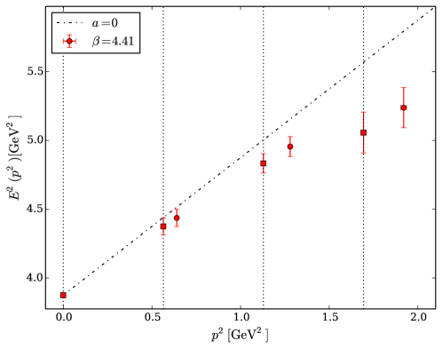
Figure 5: Interpolation to reference momenta (marked by vertical dotted lines) for the coarsest ensemble at the physical $D_{s}$ mass. The black dash-dotted line depicts the continuum dispersion relation, displayed only for reference. The closed circles show the simulated data on the coarsest ensemble ($\beta=4.41$) whilst the closed squares which lie on the vertical lines correspond to the values after the correction of eq. (38) was applied.

In figure 5 we show an example of the interpolation to the chosen reference momenta for the ensemble requiring the largest corrections (cf. table 2) for the case of the physical-mass $D_{s}$ meson. We now proceed to perform the continuum limit extrapolation of the meson energy. In figure 6 we illustrate the extrapolation of the physical $D_{s}$ meson energies for two different momenta. In both cases the extrapolated result is compatible with the energy predicted by the continuum dispersion relation (36). This procedure was repeated for all momenta and reference masses. In figure 7 we show the results for the energies after the continuum limit extrapolation for the different momenta and choices of reference rest masses. The expected continuum dispersion relation eq. (36) is recovered, indicating a good control over the continuum limit.

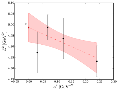
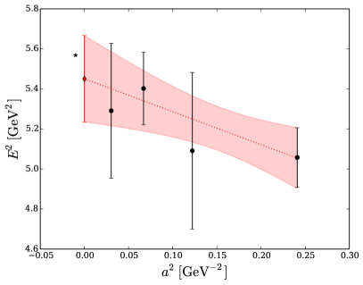
Figure 6: Continuum limit for momenta $(1,1,0)$ (left panel) and $\left(1,1,1\right)$ (right panel) for the physical-mass $D_{s}$ meson. Black circles correspond to finite lattice spacings, red diamonds to the continuum limit extrapolation; the band shows the fit ansatz, whereas the star is the energy of the meson computed using eq. (36) and the meson rest mass.

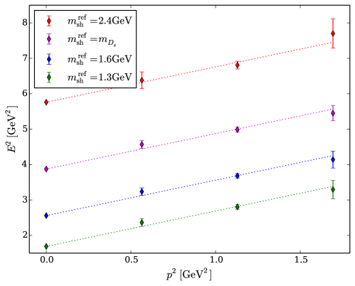
Figure 7: Continuum extrapolated results for the meson energy as a function of the momentum for the different reference masses. Each dotted line depicts the continuum dispersion relation eq. (36) for the associated reference mass. For the heaviest reference mass ($m_{sh}=2.4\mathrm{\,GeV}$), only the three finer ensembles enter the continuum limit since the heavy mass reach of the coarsest ensemble is not sufficient. This results in the larger errorbars.

5 Conclusion

This study is motivated by the need to explore new and alternative ways for discretising heavy flavours in simulations of lattice QCD: more independent predictions for heavy flavour hadronic quantities with a solid control of systematic uncertainties are urgently needed Aoki:2013ldr to make reliable predictions for SM phenomenology. To this end we explored the feasibility of Möbius domain wall fermions (MDWF) as a lattice regularisation for heavy quarks. DWF have so far been widely used as a discretisation for the light $u$, $d$ and $s$ quarks. Its desirable features are chiral symmetry to a good approximation and automatic ${\cal O}(a)$-improvement. From our simulations within quenched QCD with the tree-level improved Symanzik gauge action we have identified a point in MDWF parameter space, the domain wall height $M_{5}=1.6$, for which discretisation effects turn out to be particularly small. We demonstrated that the salient features of MDWF persist for heavy quarks as long as the bare input quark mass obeys the bound $am_{h}\lesssim 0.4$. Based on these findings we carried out a detailed scaling study of the heavy-strange dispersion relation and decay constant. Over the range of lattice cutoffs 2.0–5.7 GeV the observables were compatible with a linear scaling in $a^{2}$. At the level of precision achieved in this work, coefficients of $a^{4}$ terms were found to be almost always compatible with zero, remaining remarkably small even for the heaviest quark mass (heavier than charm) simulated. The results accumulated in this paper constitute a proof of concept for MDWF as a powerful discretisation to study charm and heavier quarks on current dynamical gauge field ensembles. This work constitutes a solid basis for RBC/UKQCD’s heavy MDWF phenomenology program Boyle:2015kyy . Nevertheless, we are considering ideas for how to improve the current setup, for example by link-smearing the MDWF kernel Cho:2015ffa ; Boyle:2015kyy .

Acknowledgements

The authors are thankful for many fruitful discussions with Y.Cho, S.Hashimoto, T. Kaneko and J. Noaki from K.E.K. and with our colleagues in the RBC and UKQCD collaborations. The research leading to these results has received funding from the European Research Council under the European Union’s Seventh Framework Programme (FP7/2007-2013) / ERC Grant agreement 279757. P.A.B. is supported in part by UK STFC Grants No. ST/M006530/1, ST/L000458/1, ST/K005790/1, and ST/K005804/1. M.S. is supported by UK EPSRC Doctoral Training Centre Grant EP/G03690X/1. The authors gratefully acknowledge computing time granted through the STFC funded DiRAC facility (grants ST/K005790/1, ST/K005804/1, ST/K000411/1, ST/H008845/1). The authors acknowledge the use of the IRIDIS High Performance Computing Facility, and associated support services at the University of Southampton, in the completion of this work.

Appendix A Topological charge evolution

In figure 8 we show the Monte Carlo histories and histograms of the topological charge restricted to the configurations on which we also determined the decay constant and the meson energies.

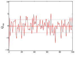
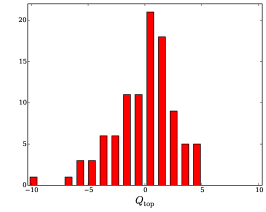
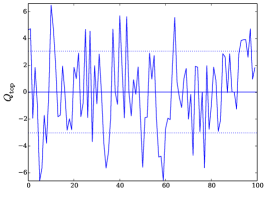
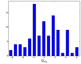
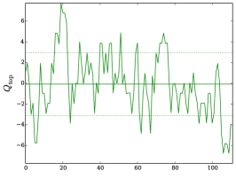
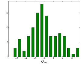
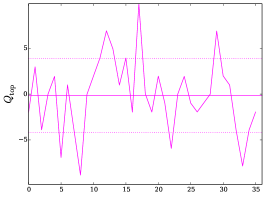
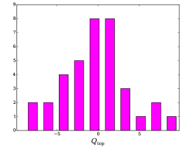
Figure 8: Topological charge evolution (left) and histograms (right) for the ensembles listed in table 1, 2 and 3. This plot only includes configurations that are decorrelated. The lattice spacing decreases from top to bottom.

Appendix B Correlator fit results

B.1 Decay constant data

tag	$am$	$af$	$\chi^{2}/\mathrm{d.o.f.}$	$am$	$af$	$\chi^{2}/\mathrm{d.o.f.}$
	$am_{s}=0.036$			$am_{s}=0.037$
ss	0.3433(16)	0.11309(57)	0.6033	0.3479(16)	0.11360(57)	0.5384
sh0	0.4738(15)	0.12710(81)	0.3443	0.4764(12)	0.12775(73)	0.4052
sh1	0.5628(14)	0.13452(83)	0.3609	0.5654(12)	0.13519(80)	0.4885
sh2	0.6448(14)	0.13960(85)	0.3471	0.6463(13)	0.13991(85)	0.3455
sh3	0.7215(13)	0.14292(88)	0.3456	0.7227(14)	0.14314(90)	0.3522
sh4	0.7938(14)	0.14480(92)	0.3825	0.7953(13)	0.14501(91)	0.2996
sh5	0.8614(15)	0.1447(10)	0.2965	0.8628(15)	0.1451(10)	0.2925
sh6	0.9254(16)	0.1439(11)	0.3610	0.9266(15)	0.1443(10)	0.3577

Table 6: Fit results for strange-strange and strange-heavy pseudoscalar masses and decay constants in lattice units for the ensembles $\beta=4.41$.

tag	$am$	$af$	$\chi^{2}/\mathrm{d.o.f.}$	$am$	$af$	$\chi^{2}/\mathrm{d.o.f.}$
	$am_{s}=0.024$			$am_{s}=0.026$
ss	0.23894(93)	0.07812(48)	0.7714	0.24883(90)	0.07926(47)	0.8466
sh0	0.3294(11)	0.08816(86)	0.8914	0.3333(11)	0.08871(85)	0.9314
sh1	0.3919(11)	0.09311(83)	0.9179	0.3955(11)	0.09381(84)	0.9530
sh2	0.4494(10)	0.09678(84)	0.9083	0.4528(11)	0.09766(90)	0.9559
sh3	0.5033(10)	0.09930(84)	0.9123	0.5063(11)	0.09997(86)	0.9319
sh4	0.5545(10)	0.10099(84)	0.8906	0.5573(10)	0.10167(82)	0.8719
sh5	0.6033(10)	0.10200(84)	0.8382	0.6059(10)	0.10269(82)	0.8245
sh6	0.6491(13)	0.1019(10)	0.8190	0.6518(12)	0.10272(97)	0.8216
sh7	0.6931(13)	0.10114(92)	0.8668	0.6962(13)	0.10248(98)	0.7454
sh8	0.7357(13)	0.10037(93)	0.7866	0.7387(13)	0.1016(10)	0.6989
sh9	0.7768(15)	0.0996(11)	0.6151	0.7793(14)	0.1004(10)	0.6358
sh10	0.8151(15)	0.0973(10)	0.6496	0.8181(15)	0.0984(11)	0.5990

Table 7: Fit results for strange-strange and strange-heavy pseudoscalar masses and decay constants in lattice units for the ensembles $\beta=4.66$.

tag	$am$	$af$	$\chi^{2}/\mathrm{d.o.f.}$	$am$	$af$	$\chi^{2}/\mathrm{d.o.f.}$
	$am_{s}=0.018$			$am_{s}=0.020$
ss	0.1773(10)	0.05630(37)	0.9652	0.1872(10)	0.05739(36)	0.8819
sh0	0.28568(95)	0.06578(66)	0.7877	0.28925(85)	0.06647(60)	0.6169
sh1	0.35566(88)	0.06991(68)	0.5133	0.35889(79)	0.07058(60)	0.4933
sh2	0.41960(90)	0.07189(70)	0.4931	0.42283(84)	0.07277(66)	0.4966
sh3	0.47922(98)	0.07256(76)	0.4981	0.48239(90)	0.07352(70)	0.5273
sh4	0.53492(93)	0.07213(78)	0.7555	0.53775(89)	0.07311(74)	0.7476
sh5	0.58831(97)	0.07138(80)	0.7290	0.59103(92)	0.07241(76)	0.7275
sh6	0.6391(10)	0.07023(81)	0.7054	0.6419(10)	0.07130(80)	0.7394
sh7	0.6872(10)	0.06876(83)	0.6944	0.6899(10)	0.06962(82)	0.7975
sh8	0.73280(96)	0.06700(65)	0.7404	0.7352(10)	0.06809(85)	0.6866

Table 8: Fit results for strange-strange and strange-heavy pseudoscalar masses and decay constants in lattice units for the ensembles $\beta=4.89$.

tag	$am$	$af$	$\chi^{2}/\mathrm{d.o.f.}$	$am$	$af$	$\chi^{2}/\mathrm{d.o.f.}$
	$am_{s}=0.0118$			$am_{s}=0.0133$
ss	0.1212(12)	0.03723(73)	0.0189	0.1288(12)	0.0382(14)	0.0080
sh0	0.1815(13)	0.04233(96)	0.0120	0.1841(13)	0.04265(98)	0.0005
sh1	0.2528(12)	0.04615(91)	0.0033	0.2552(11)	0.04659(87)	0.0042
sh2	0.3167(12)	0.04795(88)	0.0051	0.3189(12)	0.04843(84)	0.0061
sh3	0.3758(15)	0.0485(10)	0.0028	0.3778(14)	0.04891(99)	0.0027
sh4	0.4315(16)	0.0484(10)	0.0034	0.4335(14)	0.0488(10)	0.0032
sh5	0.4843(17)	0.0478(10)	0.0041	0.4862(15)	0.0483(10)	0.0038
sh6	0.5344(18)	0.0470(10)	0.0052	0.5362(16)	0.0474(10)	0.0051

Table 9: Fit results for strange-strange and strange-heavy pseudoscalar masses and decay constants in lattice units for the ensembles $\beta=5.20$.

B.2 Dispersion relation data

$\mathbf{n}$	$(0,0,0)$	$(1,0,0)$	$(1,1,0)$	$(1,1,1)$	$(0,0,0)$	$(1,0,0)$	$(1,1,0)$	$(1,1,1)$
	$am_{s}=0.034$				$am_{s}=0.036$
ss	0.3321(19)	-	-	-	0.3415(18)	-	-	-
sh0	0.4699(15)	0.619(12)	0.755(16)	0.725(68)	0.4735(14)	0.621(12)	0.757(15)	0.729(65)
sh1	0.5591(14)	0.686(10)	0.800(14)	0.793(39)	0.5624(14)	0.689(10)	0.801(13)	0.796(38)
sh2	0.6410(14)	0.750(10)	0.852(12)	0.853(32)	0.6440(14)	0.7528(98)	0.854(11)	0.856(31)
sh3	0.7174(14)	0.8143(89)	0.904(10)	0.917(25)	0.7203(14)	0.8166(87)	0.906(10)	0.920(24)
sh4	0.7894(14)	0.8763(82)	0.9566(94)	0.977(21)	0.7922(13)	0.8787(80)	0.9588(92)	0.980(20)
sh5	0.8572(14)	0.9367(78)	1.0049(90)	1.033(18)	0.8599(14)	0.9389(77)	1.0072(87)	1.035(18)
sh6	0.9209(14)	0.9935(76)	1.0561(84)	1.086(17)	0.9235(14)	0.9957(75)	1.0584(81)	1.088(16)

Table 10: Fit results for the energy of strange-strange and strange-heavy pseudoscalar mesons in lattice units as a function of the momentum for the ensemble $\beta=4.41$.

$\mathbf{n}$	$(0,0,0)$	$(1,0,0)$	$(1,1,0)$	$(1,1,1)$	$(0,0,0)$	$(1,0,0)$	$(1,1,0)$	$(1,1,1)$
	$am_{s}=0.024$				$am_{s}=0.026$
ss	0.23749(89)	-	-	-	0.24723(86)	-	-	-
sh0	0.32942(73)	0.419(16)	0.477(19)	0.583(26)	0.33328(71)	0.422(15)	0.480(19)	0.585(25)
sh1	0.39143(72)	0.473(12)	0.529(14)	0.615(32)	0.39492(71)	0.476(12)	0.532(13)	0.617(31)
sh2	0.44837(73)	0.524(11)	0.577(13)	0.650(42)	0.45163(72)	0.527(10)	0.579(12)	0.652(40)
sh3	0.50185(74)	0.572(10)	0.620(10)	0.668(48)	0.50496(72)	0.5744(98)	0.621(10)	0.672(46)
sh4	0.55252(76)	0.6178(96)	0.6603(94)	0.699(40)	0.55552(74)	0.6206(93)	0.6629(89)	0.702(38)
sh5	0.60091(78)	0.6623(91)	0.7010(85)	0.724(39)	0.60382(76)	0.6651(88)	0.7036(81)	0.727(37)
sh6	0.64723(81)	0.7054(87)	0.7407(78)	0.757(33)	0.65007(78)	0.7081(84)	0.7433(74)	0.761(32)
sh7	0.69161(83)	0.7468(84)	0.7792(73)	0.790(29)	0.69440(80)	0.7495(82)	0.7819(69)	0.794(28)
sh8	0.73410(87)	0.7868(82)	0.8166(69)	0.823(26)	0.73685(84)	0.7895(80)	0.8192(65)	0.827(25)
sh9	0.77473(90)	0.8264(84)	0.8526(66)	0.856(24)	0.77744(86)	0.8291(81)	0.8553(62)	0.859(23)
sh10	0.81346(93)	0.8632(83)	0.8873(63)	0.881(24)	0.81614(89)	0.8659(80)	0.8899(60)	0.885(23)

Table 11: Fit results for the energy of strange-strange and strange-heavy pseudoscalar mesons in lattice units as a function of the momentum for the ensemble $\beta=4.66$.

$\mathbf{n}$	$(0,0,0)$	$(1,0,0)$	$(1,1,0)$	$(1,1,1)$	$(0,0,0)$	$(1,0,0)$	$(1,1,0)$	$(1,1,1)$
	$am_{s}=0.018$				$am_{s}=0.020$
ss	0.17758(75)	-	-	-	0.18735(73)	-	-	-
sh0	0.28700(56)	0.350(10)	0.4032(50)	0.430(23)	0.29061(54)	0.3529(97)	0.4058(48)	0.432(22)
sh1	0.35690(58)	0.4085(78)	0.4562(36)	0.480(16)	0.36016(56)	0.4110(74)	0.4588(34)	0.483(15)
sh2	0.42074(60)	0.4653(66)	0.5063(35)	0.530(13)	0.42380(58)	0.4678(63)	0.5089(33)	0.533(12)
sh3	0.48047(61)	0.5186(63)	0.5542(36)	0.579(11)	0.48339(58)	0.5211(60)	0.5567(34)	0.582(11)
sh4	0.53680(65)	0.5717(59)	0.6029(32)	0.6257(90)	0.53964(62)	0.5742(56)	0.6054(31)	0.6285(87)
sh5	0.59020(67)	0.6222(57)	0.6502(30)	0.6727(84)	0.59298(64)	0.6247(54)	0.6527(28)	0.6755(81)
sh6	0.64086(69)	0.6697(58)	0.6958(28)	0.7180(80)	0.64359(66)	0.6722(55)	0.6983(26)	0.7208(77)
sh7	0.68882(72)	0.7161(55)	0.7398(26)	0.7620(84)	0.69150(68)	0.7186(53)	0.7423(24)	0.7648(80)
sh8	0.73401(74)	0.7598(56)	0.7814(25)	0.8031(83)	0.73667(70)	0.7623(53)	0.7840(23)	0.8059(79)

Table 12: Fit results for the energy of strange-strange and strange-heavy pseudoscalar mesons in lattice units as a function of the momentum for the ensemble $\beta=4.89$.

$\mathbf{n}$	$(0,0,0)$	$(1,0,0)$	$(1,1,0)$	$(1,1,1)$	$(0,0,0)$	$(1,0,0)$	$(1,1,0)$	$(1,1,1)$
	$am_{s}=0.011$				$am_{s}=0.013$
ss	0.1143(13)	-	-	-	0.1246(11)	-	-	-
sh0	0.17940(63)	0.246(13)	0.2454(78)	0.269(16)	0.18322(60)	0.248(12)	0.2495(74)	0.272(15)
sh1	0.25110(52)	0.302(12)	0.3035(51)	0.327(14)	0.25441(49)	0.304(11)	0.3074(47)	0.330(13)
sh2	0.31470(52)	0.358(11)	0.3590(43)	0.374(13)	0.31778(49)	0.360(10)	0.3625(40)	0.377(12)
sh3	0.37356(56)	0.412(11)	0.4116(38)	0.430(13)	0.37651(52)	0.414(10)	0.4148(34)	0.433(12)
sh4	0.42894(61)	0.465(11)	0.4625(36)	0.477(11)	0.43180(58)	0.466(10)	0.4656(32)	0.481(11)
sh5	0.48138(67)	0.516(10)	0.5114(35)	0.524(10)	0.48419(62)	0.517(10)	0.5143(31)	0.527(10)
sh6	0.53114(72)	0.564(11)	0.5582(34)	0.5689(99)	0.53390(67)	0.566(10)	0.5611(30)	0.5723(95)

Table 13: Fit results for the energy of strange-strange and strange-heavy pseudoscalar mesons in lattice units as a function of the momentum for the ensemble $\beta=5.20$.

References

- (1) G. P. Lepage and B. A. Thacker, Effective Lagrangians for Simulating Heavy Quark Systems, Nucl. Phys. Proc. Suppl. 4 (1988) 199.
- (2) B. A. Thacker and G. P. Lepage, Heavy quark bound states in lattice QCD, Phys. Rev. D43 (1991) 196–208.
- (3) E. Eichten and B. R. Hill, An Effective Field Theory for the Calculation of Matrix Elements Involving Heavy Quarks, Phys. Lett. B234 (1990) 511.
- (4) ALPHA collaboration, J. Heitger and R. Sommer, Nonperturbative heavy quark effective theory, JHEP 02 (2004) 022, [hep-lat/0310035].
- (5) A. X. El-Khadra, A. S. Kronfeld and P. B. Mackenzie, Massive fermions in lattice gauge theory, Phys. Rev. D55 (1997) 3933–3957, [hep-lat/9604004].
- (6) N. H. Christ, M. Li and H.-W. Lin, Relativistic Heavy Quark Effective Action, Phys. Rev. D76 (2007) 074505, [hep-lat/0608006].
- (7) H.-W. Lin and N. Christ, Non-perturbatively Determined Relativistic Heavy Quark Action, Phys. Rev. D76 (2007) 074506, [hep-lat/0608005].
- (8) S. Aoki, Y. Kuramashi and S.-i. Tominaga, Relativistic heavy quarks on the lattice, Prog. Theor. Phys. 109 (2003) 383–413, [hep-lat/0107009].
- (9) HPQCD, UKQCD collaboration, E. Follana, Q. Mason, C. Davies, K. Hornbostel, G. P. Lepage, J. Shigemitsu et al., Highly improved staggered quarks on the lattice, with applications to charm physics, Phys. Rev. D75 (2007) 054502, [hep-lat/0610092].
- (10) ETM collaboration, B. Blossier et al., A Proposal for B-physics on current lattices, JHEP 04 (2010) 049, [0909.3187].
- (11) C. T. Sachrajda, Long-distance contributions to flavour-changing processes, PoS LATTICE2014 (2015) 023, [1503.01691].
- (12) Y.-G. Cho, S. Hashimoto, A. Jüttner, T. Kaneko, M. Marinkovic, J.-I. Noaki et al., Improved lattice fermion action for heavy quarks, JHEP 05 (2015) 072, [1504.01630].
- (13) D. B. Kaplan, A Method for simulating chiral fermions on the lattice, Phys. Lett. B288 (1992) 342–347, [hep-lat/9206013].
- (14) Y. Shamir, Chiral fermions from lattice boundaries, Nucl. Phys. B406 (1993) 90–106, [hep-lat/9303005].
- (15) R. C. Brower, H. Neff and K. Orginos, Möbius fermions: Improved domain wall chiral fermions, Nucl.Phys.Proc.Suppl. 140 (2005) 686–688, [hep-lat/0409118].
- (16) R. Brower, H. Neff and K. Orginos, Möbius fermions, Nucl.Phys.Proc.Suppl. 153 (2006) 191–198, [hep-lat/0511031].
- (17) R. C. Brower, H. Neff and K. Orginos, The Móbius Domain Wall Fermion Algorithm, 1206.5214.
- (18) Alpha collaboration, R. Frezzotti, P. A. Grassi, S. Sint and P. Weisz, Lattice QCD with a chirally twisted mass term, JHEP 08 (2001) 058, [hep-lat/0101001].
- (19) TWQCD collaboration, W.-P. Chen, Y.-C. Chen, T.-W. Chiu, H.-Y. Chou, T.-S. Guu and T.-H. Hsieh, Decay Constants of Pseudoscalar -mesons in Lattice QCD with Domain-Wall Fermion, Phys. Lett. B736 (2014) 231–236, [1404.3648].
- (20) H.-W. Lin, S. Ohta, A. Soni and N. Yamada, Charm as a domain wall fermion in quenched lattice QCD, Phys. Rev. D74 (2006) 114506, [hep-lat/0607035].
- (21) M. Creutz, Overrelaxation and Monte Carlo Simulation, Phys. Rev. D36 (1987) 515.
- (22) A. D. Kennedy and B. J. Pendleton, Improved Heat Bath Method for Monte Carlo Calculations in Lattice Gauge Theories, Phys. Lett. B156 (1985) 393–399.
- (23) N. Cabibbo and E. Marinari, A New Method for Updating SU(N) Matrices in Computer Simulations of Gauge Theories, Phys. Lett. B119 (1982) 387–390.
- (24) S. Duane, A. D. Kennedy, B. J. Pendleton and D. Roweth, Hybrid Monte Carlo, Phys. Lett. B195 (1987) 216–222.
- (25) L. Del Debbio, G. M. Manca and E. Vicari, Critical slowing down of topological modes, Phys. Lett. B594 (2004) 315–323, [hep-lat/0403001].
- (26) ALPHA collaboration, S. Schaefer, R. Sommer and F. Virotta, Critical slowing down and error analysis in lattice QCD simulations, Nucl. Phys. B845 (2011) 93–119, [1009.5228].
- (27) J. Flynn, A. Jüttner, A. Lawson and F. Sanfilippo, Precision study of critical slowing down in lattice simulations of the model, 1504.06292.
- (28) H. Neuberger, Vector - like gauge theories with almost massless fermions on the lattice, Phys. Rev. D57 (1998) 5417–5433, [hep-lat/9710089].
- (29) H. Neuberger, Exactly massless quarks on the lattice, Phys. Lett. B417 (1998) 141–144, [hep-lat/9707022].
- (30) RBC, UKQCD collaboration, D. J. Antonio et al., Localization and chiral symmetry in three flavor domain wall QCD, Phys. Rev. D77 (2008) 014509, [0705.2340].
- (31) K. Jansen and M. Schmaltz, Critical momenta of lattice chiral fermions, Phys. Lett. B296 (1992) 374–378, [hep-lat/9209002].
- (32) D. B. Kaplan, Chiral Symmetry and Lattice Fermions, in Modern perspectives in lattice QCD: Quantum field theory and high performance computing. Proceedings, International School, 93rd Session, Les Houches, France, August 3-28, 2009, pp. 223–272, 2009. 0912.2560.
- (33) N. H. Christ and G. Liu, Massive domain wall fermions, Nucl. Phys. Proc. Suppl. 129 (2004) 272–274.
- (34) G.-f. Liu, Quark eigenmodes and lattice QCD. PhD thesis, Columbia U., 2003.
- (35) RBC, UKQCD collaboration, T. Blum et al., Domain wall QCD with physical quark masses, 1411.7017.
- (36) G. Curci, P. Menotti and G. Paffuti, Symanzik’s Improved Lagrangian for Lattice Gauge Theory, Phys.Lett. B130 (1983) 205.
- (37) M. Lüscher and P. Weisz, On-Shell Improved Lattice Gauge Theories, Commun. Math. Phys. 97 (1985) 59.
- (38) SciDAC, LHPC, UKQCD collaboration, R. G. Edwards and B. Joo, The Chroma software system for lattice QCD, Nucl. Phys. Proc. Suppl. 140 (2005) 832, [hep-lat/0409003].
- (39) F. Sanfilippo. https://github.com/sunpho84/nissa.
- (40) M. Lüscher, Properties and uses of the Wilson flow in lattice QCD, JHEP 08 (2010) 071, [1006.4518].
- (41) S. Borsanyi et al., High-precision scale setting in lattice QCD, JHEP 09 (2012) 010, [1203.4469].
- (42) R. Hudspith. https://github.com/RJhudspith/GLU.
- (43) ALPHA collaboration, U. Wolff, Monte Carlo errors with less errors, Comput. Phys. Commun. 156 (2004) 143–153, [hep-lat/0306017].
- (44) P. A. Boyle, Conserved currents for Möbius Domain Wall Fermions, 1411.5728.
- (45) S. Gusken, U. Low, K. H. Mutter, R. Sommer, A. Patel and K. Schilling, Nonsinglet Axial Vector Couplings of the Baryon Octet in Lattice QCD, Phys. Lett. B227 (1989) 266.
- (46) C. Alexandrou, F. Jegerlehner, S. Gusken, K. Schilling and R. Sommer, B meson properties from lattice QCD, Phys. Lett. B256 (1991) 60–67.
- (47) UKQCD collaboration, C. R. Allton et al., Gauge invariant smearing and matrix correlators using Wilson fermions at Beta = 6.2, Phys. Rev. D47 (1993) 5128–5137, [hep-lat/9303009].
- (48) UKQCD collaboration, M. Foster and C. Michael, Quark mass dependence of hadron masses from lattice QCD, Phys. Rev. D59 (1999) 074503, [hep-lat/9810021].
- (49) UKQCD collaboration, C. McNeile and C. Michael, Decay width of light quark hybrid meson from the lattice, Phys. Rev. D73 (2006) 074506, [hep-lat/0603007].
- (50) P. A. Boyle, A. Jüttner, C. Kelly and R. D. Kenway, Use of stochastic sources for the lattice determination of light quark physics, JHEP 08 (2008) 086, [0804.1501].
- (51) A. Jüttner and M. Della Morte, Heavy quark propagators with improved precision using domain decomposition, PoS LAT2005 (2006) 204, [hep-lat/0508023].
- (52) A. Borici, Truncated overlap fermions, Nucl. Phys. Proc. Suppl. 83 (2000) 771–773, [hep-lat/9909057].
- (53) A. Borici, Truncated overlap fermions: The Link between overlap and domain wall fermions, in Lattice fermions and structure of the vacuum. Proceedings, NATO Advanced Research Workshop, Dubna, Russia, October 5-9, 1999, pp. 41–52, 1999. hep-lat/9912040.
- (54) A. Kennedy, Algorithms for dynamical fermions, hep-lat/0607038.
- (55) P. Hernandez, K. Jansen and M. Lüscher, Locality properties of Neuberger’s lattice Dirac operator, Nucl. Phys. B552 (1999) 363–378, [hep-lat/9808010].
- (56) C. T. H. Davies, C. McNeile, E. Follana, G. P. Lepage, H. Na and J. Shigemitsu, Update: Precision decay constant from full lattice QCD using very fine lattices, Phys. Rev. D82 (2010) 114504, [1008.4018].
- (57) Particle Data Group collaboration, K. A. Olive et al., Review of Particle Physics, Chin. Phys. C38 (2014) 090001.
- (58) S. Aoki et al., Review of lattice results concerning low-energy particle physics, Eur. Phys. J. C74 (2014) 2890, [1310.8555].
- (59) P. Boyle, L. Del Debbio, A. Khamseh, A. Jüttner, F. Sanfilippo and J. T. Tsang, Domain Wall Charm Physics with Physical Pion Masses: Decay constants, bag and parameters, in Proceedings, 33rd International Symposium on Lattice Field Theory (Lattice 2015), 2015. 1511.09328.