Topographical pathways guide chemical microswimmers

Abstract

Achieving control over the directionality of active colloids is essential for their use in practical applications such as cargo carriers in microfluidic devices. So far, guidance of spherical Janus colloids was mainly realized using specially engineered magnetic multilayer coatings combined with external magnetic fields. Here, we demonstrate that step-like sub-micron topographical features can be used as reliable docking and guiding devices for chemically active spherical Janus colloids. For various topographic features (stripes, squares or circular posts) docking of the colloid at the feature edge is robust and reliable. Furthermore, the colloids move along the edges for significantly long times, which systematically increase with fuel concentration. The observed phenomenology is qualitatively captured by a simple continuum model of self-diffusiophoresis near confining boundaries, indicating that the chemical activity and associated hydrodynamic interactions with the nearby topography are the main physical ingredients behind the observed behaviour.

I Introduction

Catalytically active micron-sized objects can self-propel by various mechanisms, including bubble ejection, diffusio-, and electro-phoresis, when parts of their surface catalyze a chemical reaction in a surrounding liquid. In future, such chemically active micromotors may serve as autonomous carriers working within microfluidic devices to fulfill complex tasks Wang et al. (2013); Sánchez et al. (2015); Wang (2013). However, in order to achieve this goal, it is essential to gain robust control over the directionality of particle motion. Although it has been more than a decade since motile chemically active colloids were first reported Paxton et al. (2004); Kline et al. (2005); Fournier-Bidoz et al. (2005); Baraban et al. (2012) this remains a challenging issue, in particular for the case of spherical particles.

Two main methods of guidance have been so far employed with varying degrees of success. The first one uses controlled spatial gradients of “fuel” concentration. This approach suffers, however, from severe difficulties in creating and maintaining chemical gradients, and the spatial precision of guidance remains rather poor Hong et al. (2007); Baraban et al. (2013); Dey et al. (2013); Saha et al. (2014); Peng et al. (2015). The second approach relies upon the use of external magnetic fields in combination with particles with suitably designed magnetic coatings or inclusions Kline et al. (2005); Solovev et al. (2010). This proved to be a very precise guidance mechanism which could be employed straightforwardly for the case of rod-like particles Khalil et al. (2013) but difficult to extend to the case of spherical colloids, where it requires sophisticated engineering of multilayer magnetic coatings Baraban et al. (2012); Ulbrich et al. (2010); Albrecht et al. (2005); Gunther et al. (2010). Additionally, individualized guidance of specific particles is difficult to achieve without complicated external apparatus and feedback loops Khalil et al. (2015). The advantages of autonomous operation are thereby significantly hindered.

While these methods are quite general in their applicability, we note here that the synthetic micromotors are, in general, density mismatched with the suspending medium and therefore tend to sediment and move near surfaces. Furthermore, even in situations in which sedimentation can be neglected (e.g., in the case of neutrally buoyant swimmers) the presence of confining surfaces has profound consequences on swimming trajectories, as discussed below. Theoretical studies have shown that long range hydrodynamic interactions between microswimmers and nearby surfaces Evans and Lauga (2010); Spagnolie and Lauga (2012) can give rise to trapping at the walls or circular motion. Moreover, a theoretical study of a model active Janus colloid moving near a planar inert wall has revealed complex behaviour, including novel sliding and hovering steady states Uspal et al. (2015). Experimentally, wall-bounded motion of active Janus particles was evidenced in the study by Bechinger et al. Volpe et al. (2011), while capture into orbital trajectories of active bi-metallic rods by large spherical beads or of Janus colloids in colloidal crystals has recently been reported Brown et al. (2016); Takagi et al. (2016). Capture of microswimmers by spherical obstacles via hydrodynamic interactions has been modeled theoretically by Lauga et al. Spagnolie et al. (2015).

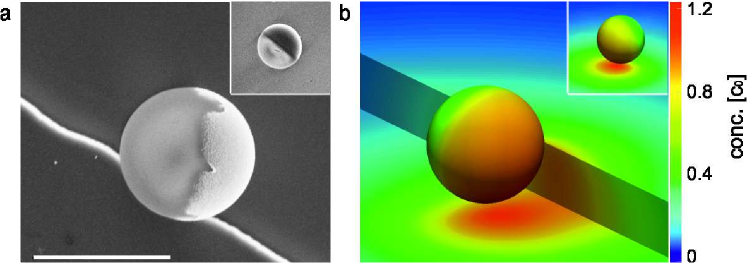
Figure 1: Janus microswimmers near sub-micron steps. (a) Top view SEM image of a spherical Janus motor on a Silicon substrate with a Silicon step. The lighter part of the Janus particle corresponds to Pt, while the gray part is the SiO₂; scale bar corresponds to 2 $\mathrm{\mu m}$. (b) Color-coded steady-state distribution $c(\mathbf{r})$ of reaction products around a half covered Janus particle at an inert wall and a step with height $h_{step}=R$, where $R$ is the particle radius. The color map shows $c(\mathbf{r})$ at the surfaces of the particle and substrate, and is represented in units of $c_{0}$ defined in Methods. The insets show the particles on a flat surface.

This intrinsic tendency of the active swimmers to operate near bounding surfaces motivated us to examine whether it can be further exploited to achieve directional guidance of chemically active microswimmers by endowing the wall with small height step-like topographical features, as shown in Fig. 1, which the particles can eventually exploit as pathways. Recently, Palacci et al. have shown that shallow rectangular grooves can efficiently guide photocatalytic hematite swimmers that have size comparable with the width of the groove Palacci et al. (2013). Because of the strong lateral confinement, it is hard to discriminate between the different physical contributions which lead to particle guidance. Here we use a much less restrictive geometry – a shallow topographical step – and it is a priori not clear whether a self-phoretic swimmer can follow such features. We report experimental evidence that Janus microswimmers can follow step-like topographical features that are only a fraction of the particle radius in height. This is, in some sense, similar to the strategy employed in natural systems well below the microscale: within cells, protein motors such as myosin, kinesin and dynein use binding to microtubules to switch to directional motion Howard et al. (1989); Howard (2002). The guidance of microswimmers through patterned device topography that we propose and demonstrate in this study may pave the way for new methods of self-propeller motion control based upon patterned walls.

II Results

II.1 Dynamics of Janus microswimmers at a planar wall

Janus particles are fabricated by vapor deposition of a thin layer of Pt (7 nm) on SiO₂ particles (diameters of approximately 2 and 5 $\mathrm{\mu m}$). For details on the fabrication see Methods section. Scanning electron microscopy (SEM) images of a Janus particle at the step edge are shown in Fig. 1a, while Fig. 1b illustrates numerically calculated steady-state distributions of the reaction products around a model half Pt-covered Janus sphere near a step.

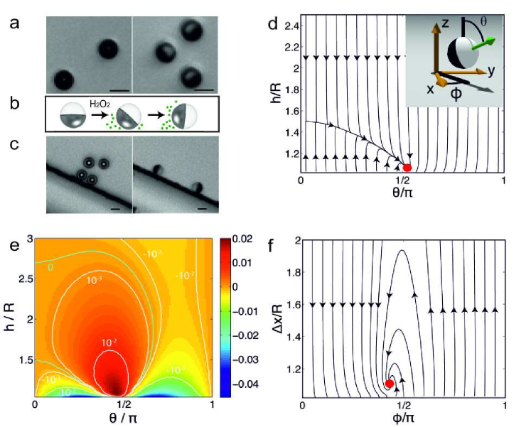
Figure 2: Behavior of Janus particles near planar surfaces. (a) Particles which sedimented to the bottom surface in a water suspension (inactive system) tend to align with their Pt caps facing downwards, which is more pronounced for larger particles. The Pt caps ($\rho$ = 21.45 g/cm³), which are much denser than the silica parts of the particles, render them bottom-heavy (in the image one sees transparent SiO₂ on top of heavily absorbing Pt). However, on addition of H₂O₂ (active system), the particles reorient their symmetry axis parallel to the bottom surface and can be seen as half covered circles in the right micrograph in (a), where dark semi-spheres correspond to the Pt cap, and the SiO₂ parts which do not absorb the light appear lighter. (b) Schematic of a particle rotating from bottom-down configuration upon peroxide addition. (c) Micrograph of Janus colloids ($R=2.5~{}\mathrm{\mu m}$) in the vicinity of the step with height $h_{step}=800~{}\mathrm{nm}$. In the absence of H₂O₂ (left image), the step (seen as a black line) has no influence on the orientation of the particles, (their caps are facing downwards, same as far from the step). Upon addition of fuel (right image), the particles orient with their symmetry axis parallel to both the bottom surface and the step. Scale bars in (a) and (c) correspond to 5 $\mathrm{\mu m}$. (d) The phase portrait for a bottom-heavy (see Supplementary Note 1) particle with $R=2.5~{}\mathrm{\mu m}$ at an infinite planar wall oriented with its normal parallel to the direction of gravity. The phase portrait is calculated at $b_{inert}/b_{cap}=0.3$, $b_{w}/b_{cap}=-0.2$, where $b_{inert}$ and $b_{cap}$ are the surface mobilities (see Methods for details) at the inert and catalytic faces of the particle respectively, and $b_{w}$ is the surface mobility at the wall. (The phase portrait for $R=1.0~{}\mathrm{\mu m}$ is shown in Supplementary Fig. 2) The phase portrait indicates that a particle will rotate to its steady state orientation $\theta=\theta_{eq}\approx 90^{\circ}$ for all initial conditions. The inset represents a schematic diagram of the system: a Janus sphere of radius $R$ is placed at distance $h$ above an inert wall; $\theta$ describes the orientation of the particle’s cap with respect to the wall normal. $\Delta x$ is the distance from the step to the particle center and $\phi$ is the cap orientation with respect to the step normal. (e) The rate of rotation $\dot{\theta}=−\Omega_{x}/\Omega_{0}$ of a particle with $R=2.5~{}\mathrm{\mu m}$ above a planar substrate, including contributions from activity, gravity, and chemi-osmotic flows on the substrate. This function is the sum of panels (a), (e), and (f) in Fig. 3. (f) Phase portrait similar to the one in (d) but in absence of gravity; all other parameters are as in (d). This portrait is supposed to capture qualitatively the effect of the vertical step wall.

Initially, the particles are introduced to the system with no H₂O₂ present, and due to their weight they sediment near the bottom surface. After sedimentation, we find the particles uniformly distributed over the substrate, and most of the 5 $\mathrm{\mu m}$ particles have their much denser (compared with the SiO₂ cores) Pt-caps oriented downwards (Fig. 2a, left), while smaller particles have a wider distribution of orientations. The particles are seen in the same focal plane of the microscope, which indicates that they are at similar vertical distances from the substrate. Upon addition of H₂O₂ to the system, we observe that the Pt-caps of the microswimmers are oriented parallel to the substrate plane (see Fig. 2a, right and b; and for the definition of the geometrical parameters see Supplementary Figure 1). Following this re-orientation, the microswimmers start moving parallel to the substrate in the direction away from the catalytic caps. In Fig. 2c we show snapshots from an optical microscopy video recording of Janus microswimmers in the vicinity of a step with $h_{step}=800~{}\mathrm{nm}$. Similarly to the case depicted in Fig. 2a (left), in the absence of H₂O₂ the particles are oriented cap-down. After addition of hydrogen peroxide, the particle caps turn away from the substrate and the particles start moving in random directions until some of them encounter a step; if the step is sufficiently tall (depending on the particle size) the particles stop, reorient, and continue self-propelling along it. These observations confirm our hypothesis that the presence of a side step near the active microswimmers, even if small compared to the particle radius, has an influence on their orientation.

We show that this behavior (alignment with both the wall and the step) is captured by a simple model of neutral self-diffusiophoresis (see Methods section for details of the model), in which we assume that the activity of the Janus particle is captured by the release of a neutral solute (O₂ molecules) at a constant rate from its catalytic cap Golestanian et al. (2005). The resulting anisotropic solute distribution around the particle drives a surface flow in a thin layer surrounding the particle, leading to its directed motion Golestanian et al. (2005); Golestanian (2009). The catalytically active particle has several types of interaction with a nearby impermeable wall. The particle drives long range flows in the suspending solution. These flows are reflected from the wall, coupling back to the particle (“hydrodynamic interaction”). Secondly, the particle’s self-generated solute gradient is modified by the presence of the wall. The wall-induced modification of the solute concentration field can contribute to translation and rotation of the particle (“phoretic interaction”). In particular, when the solute interacts more weakly with the inert region of the particle than with the catalytic cap and both interactions are repulsive (see Methods for details), the confinement and accumulation of solute near the substrate tends to drive rotation of the cap away from the substrate. On the other hand, the bottom-heaviness of the particle, along with the hydrodynamic interaction of the particle with the substrate, tends to drive the rotation of the cap toward the substrate. Finally, the inhomogeneous solute distribution along the wall induces a solute gradient driven “chemi-osmotic” flow along the substrate. For repulsive solute-substrate interactions, this surface slip velocity is directed quasi-radially inward toward the particle, driving a particle-uplifting flow in the suspending solution, as well as causing the particle cap to rotate away from the substrate. For attractive solute-substrate interactions the opposite directions of flows apply. Numerical analysis of this model system shows that, depending on the relative strengths of these interactions (i.e. the parameters characterizing the surface chemistry of the particle and the wall), the various contributions to rotation discussed above may balance at a steady height $h_{eq}$ and orientation $\theta_{eq}\approx 90^{\circ}$, and that this steady state is robust and stable against perturbations in height and orientation. The particle cap orientation would therefore evolve to $\theta_{eq}\approx 90^{\circ}$ (i.e., the symmetry axis almost parallel to the substrate) from nearly all initial orientations, including a cap-down one. In Fig. 2d, a phase portrait shows the dynamical evolution of particle height and orientation, and the color-coded rate of rotation $\dot{\theta}=−\Omega_{x}$ is depicted in Fig. 2e. The steady state (red dot) clearly has a large basin of attraction. We note that our numerical calculations were carried out for $h/R\geq 1.02$. Therefore, some trajectories in the region of the cap up ($\theta=180^{\circ}$) orientation encounter a numerical cutoff. However, based on the structure of the phase portrait, we expect such trajectories to roll toward $\theta\approx 90^{\circ}$ after close encounter with the wall.

Figure 3: Various contributions to particle angular velocity. (a) Contribution from self-diffusiophoresis $-\Omega_{x}^{a}/\Omega_{0}$ (see Supplementary Note 2 and Eq. (2) therein) as a function of height $h/R$ and orientation $\theta$ for half covered Janus microswimmer and unequal surface mobilities $b_{inert}/b_{cap}=0.3$. Throughout, white curves correspond to constant values of $\Omega_{x}^{a}$. Note that, by definition, panel (a) is the sum of panels (b), (c), and (d). (b) Contribution $-\Omega_{x}^{a,hi}/\Omega_{0}$ obtained by using the free space number density of solute distribution $c^{fs}(\mathbf{r})$ around the particle, i.e., neglecting the influence of the wall on the number density of solute, but including the influence of the wall on the hydrodynamic flow. (c) Contribution $-\Omega_{x}^{a,sol}/\Omega_{0}$ obtained by using the free space hydrodynamics stress tensor $\boldsymbol{\sigma^{\prime}}^{fs}$ in the dual Stokes problems employed in the reciprocal theorem, i.e., neglecting the effect of the wall on the hydrodynamics, but including the chemical effect. (d) Contribution $-\Omega_{x}^{\delta\delta}/\Omega_{0}$ due to higher order coupling between the two effects. (e) Contribution $-\Omega_{x}^{a,g}/\Omega_{0}$ to rate of rotation from the bottom-heaviness of the particle. (f) Chemio-osmotic contribution $-\Omega_{x}^{a,ws}/\Omega_{0}$ due to the activity-induced phoretic slip at the wall calculated at $b_{w}/b_{cap}=-0.2$.

If a particle as above would encounter now a second vertical side wall, numerical simulations for the same interaction parameters show (see Fig. 2f) that for this wall, for which gravity now plays no role, a similar sliding along the wall attractor emerges with $\phi_{eq}\approx 90^{\circ}$, i.e. with the particle oriented with its axis almost parallel to the vertical wall. The combination of the two sliding states thus aligns the axis of the particle along the edge formed by the two walls. Note that although this second fixed point appears to have a smaller basin of attraction, it should capture the whole $\phi\leq 90^{\circ}$ range. A particle on a trajectory that “crashes” into the vertical wall would diffuse along the wall until it reaches the basin of attraction in the vicinity of $\phi_{eq}\approx 90^{\circ}$. While the argument is developed for the superposition of two infinite planar walls, we expect that similar features may occur for a vertical step with finite height.

Within our model, we can isolate and quantify the various wall-induced contributions to particle motion discussed above. The mathematical details of the decomposition are given in Supplementary Note 2. In Fig. 3b we show the contribution to the rate of rotation $\dot{\theta}$ of the particle from hydrodynamic interaction (HI) with the wall as a function of particle height and orientation. Hydrodynamic interactions always rotate the particle cap towards the wall. Therefore, for the particular combination of parameters used in this work, hydrodynamic interactions cannot by themselves produce a steady orientation $\theta_{eq}\approx 90^{\circ}$. On the other hand, phoretic interactions always rotate the cap away from the wall, as described above (Fig. 3c). Therefore, the interplay of hydrodynamic and phoretic interactions can produce a curve with $\dot{\theta}=0$ in the region of $\theta_{eq}\approx 90^{\circ}$ (Fig. 3a). Moreover, the contributions of bottom-heaviness (Fig. 3e) and chemi-osmotic flow on the wall (Fig. 3f) to the angular velocity are comparable in magnitude to the contributions from hydrodynamic and phoretic interactions. Therefore, for the parameters used in this work, all of these effects are important in determining the emergence and location of a “sliding state” attractor. The surface chemistry parameters were chosen as providing the best fit to the experimental observations of the two sliding states (above a substrate and along a side wall).

Model	Best fit parameters	$h_{eq}/R$, no gravity	$\theta_{eq}$, no gravity	$h_{eq}/R$, with gravity	$\theta_{eq}$, with gravity
	$b_{inert}/b_{cap}=0.3$
Full Model	$b_{wall}/b_{cap}=-0.2$	1.11	$77.9^{\circ}$	1.06	$94.8^{\circ}$
	$b_{cap}<0$
Squirmer, first
two squirming	$B_{2}/B_{1}=0.3$	1.64	$102^{\circ}$	$<1.02$	$\approx 45^{\circ}$
modes only
Effective	$b_{inert}/b_{cap}=-0.8$
squirmer	$b_{cap}<0$	1.063	$69.7^{\circ}$	1.09	$65.3^{\circ}$

Table 1: Comparison of full model with two hydrodynamics-only models. For each model, we list the parameters that give the best fit to the experimental observations. For each model and set of best fit parameters, we give the height and orientation of the particle when it is in a “sliding state” above a planar wall in both the presence of gravity (corresponding to motion above a substrate) and the absence of gravity (corresponding to motion near a side wall). Experimentally, it is observed that $\theta_{eq}\approx 90^{\circ}$ in both cases. Of the three models, the full model shows the best fit with these experimental observations. For the squirmer with only the first two squirming modes, there are clear signs of an attractor with $h_{eq}/R$ below the numerical cut-off of $h/R=1.02$ in the presence of gravity, but this attractor has $\theta_{eq}$ far from $90^{\circ}$ (see also Supplementary Note 3 and Supplementary Table 1). The best fit effective squirmer agrees moderately well with the experimental observations. However, the orientation of the sliding seems significantly different from the experiment, and, as discussed in Supplementary Note 3 and Supplementary Table 2, the best fit parameters correspond to an unrealistically large force dipole.

As noted above our model includes several types of interaction of the particle with the wall. However, many theoretical Spagnolie et al. (2015) and experimental Volpe et al. (2011); Brown et al. (2016) studies have sought to characterize the interaction of active particles and solid boundaries strictly in terms of effective hydrodynamic interactions (HI). It is therefore interesting to compare our full model against the best fit results from effective HI models. We consider two such approaches, the details of which are given in Supplementary Note 3. Briefly, in the first approach, we use the classical “squirmer” model, and specify a priori the amplitude of the first two squirming modes. Higher order modes are taken to have zero amplitude. In the second approach, we consider the “effective squirmer” obtained within our model by neglecting phoretic and chemi-osmotic effects. The “effective squirmer” approach intrinsically covers a broad range of squirming mode amplitudes. In Table 1, we show that the results of the full model match the experimental observations significantly better than the best results of the two HI-only approaches.

II.2 Dynamics of Janus microswimmers at a rectangular step

We designed a system with microfabricated 3D structures by patterning of photoresist through a circular or square mask, followed by e-beam deposition of the required material (Si or SiO₂ in our case), and then removal of the developed photoresist resulting in desired structures (for detailed information see Methods). Depending on the use of positive or negative photoresist we obtain patterns with posts or wells of different shapes (see Supplementary Figure 5). The height of the features patterned on a substrate is tunable in a wide range; in this study, we have tested step heights $h_{step}$ between 100 and 1000 nm.

II.2.1 Characterization of particle trajectories approaching a step

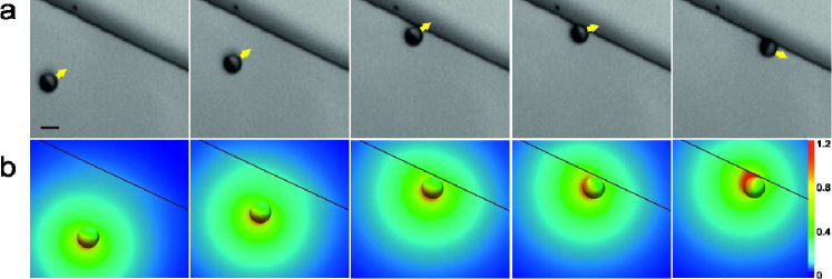
Figure 4: Effect of 800 nm height step on the dynamics of a Janus microswimmer. (a) An active Janus particle approaching a step; after direct contact with the step, it reorients until its propulsion axis is parallel to the step. $R=2.5~{}\mathrm{\mu m}$, $h_{step}=800~{}\mathrm{nm}$, 2.5 % vol. H₂O₂. (b) Numerically calculated steady-state distribution $c(\mathbf{r})$ of reaction products around half catalyst-covered Janus sphere as a function of the step distance and the cap orientation with respect to the step. The color map shows $c(\mathbf{r})$ at the surfaces of the particle and substrate; $c(\mathbf{r})$ is in units of $c_{0}$ (see Methods). Scale bar correspond to 5 $\mathrm{\mu m}$.

Fig. 4a shows snapshots of a typical trajectory of a microswimmer moving toward a step at almost perpendicular direction. Once the particle hits the step (Fig. 4a, third panel) it starts reorienting its axis (Fig. 4a, forth panel) toward the direction along the step (Fig. 4a, fifth panel). We observe that in most cases the complete process of reorientation takes less than ten seconds, independent of the initial angle at which the particle approaches the step. Within the resolution of our experimental equipment, we do not observe any systematic deflection in the trajectory of the particle in the vicinity of the steps. Therefore we conclude that if any long range effective interaction exists between the particles and the steps, it must be very weak. This observation is reproduced by our numerical model: we calculate that the effects of a wall on the velocity of a particle are negligible when the particle is more than three radii away from the wall (Supplementary Fig. 4 and Supplementary Note 4). We thus attribute the suppression, upon collision with the step, of the motion of the particles normal to the step solely to steric interactions.

In Fig. 4b we present the distribution of the reaction products around a microswimmer calculated numerically for particle positions and orientations approximately corresponding to those shown in the experimental micrographs in Fig. 4a. When the particle is far away from the step (Fig. 4b, first and second panels), approaching it in a head-on direction, the generated concentration field confirms the expected mirror symmetry with respect to the plane defined by the motion axis and the normal to the substrate. As the result of this symmetry there are no activity induced rotations and the particle stays on its head-on track (up to Brownian rotational diffusion) toward the step. However, closer to the step a head-on collision becomes unstable to small fluctuations of the propulsion axis as any such fluctuation gets amplified by the buildup of asymmetric product distribution in the region between one side of the particle and the step (Fig. 4b, forth panel). This eventually leads to the reorientation of the motion axis parallel to the step (Fig. 4b, fifth panel).

II.2.2 Effects of the step height on the capture efficiency

We observe that submicron steps are able to capture and guide particles as shown in Fig. 5 (insets). To evaluate the minimum height $h_{step}^{*}$ that can still influence the trajectory of the particles, we fabricated a set of patterns with $h_{step}$ varying in a range from 100 nm to 1000 nm. The results for the two different particle sizes show that $h_{step}^{*}$ decreases as the particle size increases. In Fig. 5 we summarize the responses of $R=1.0~{}\mathrm{\mu m}$ and $R=2.5~{}\mathrm{\mu m}$ active particles to steps of different heights. Both types of particles could swim over the step of 100 nm height. For $R=2.5~{}\mathrm{\mu m}$ particles steps of height 200 nm already ensure about 90% docking of particles upon collision with the step, while a significant fraction of the $R=1.0~{}\mathrm{\mu m}$ particles managed to pass over the 200 nm high step, and 400 nm high steps were required for efficient docking. From Fig. 5 we infer that $h_{step}^{*}/R$ is smaller for larger particles.

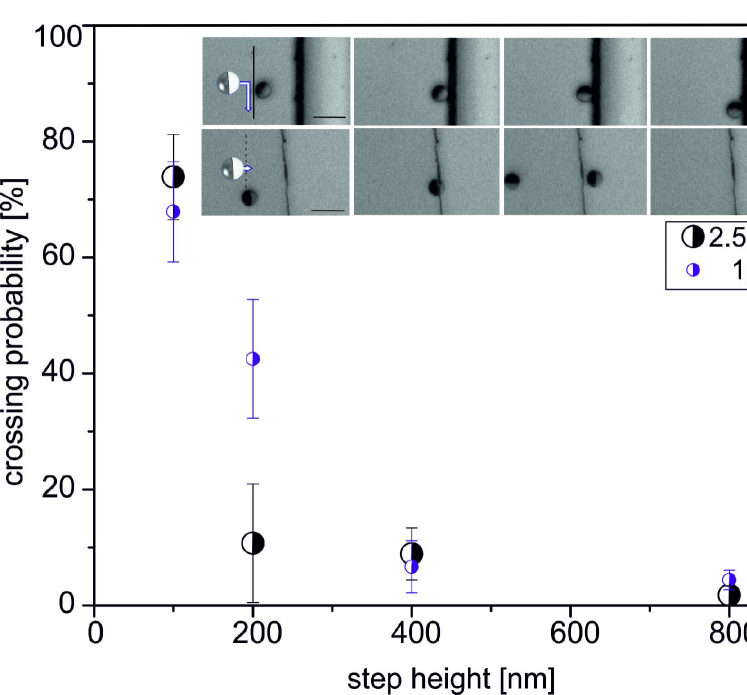
Figure 5: Sub-micron steps as rectifiers of active particles’ trajectories. A summary of the crossing behavior of Janus SiO₂ microswimmers of different sizes at several values of $h_{step}$; the error bars are standard errors of the mean. Inset: A sequence of micrographs showing a Janus particle with $R=2.5~{}\mathrm{\mu m}$ approaching a step with $h_{step}=800$ nm, reorienting and then moving parallel to it. Micrograph sequence of a Janus particle, $R=2.5~{}\mathrm{\mu m}$, passing over a step, $h_{step}=100$ nm. All scale bars correspond to 10 $\mathrm{\mu m}$.

Having estimated the threshold values $h_{step}^{*}$ for particle trapping, we now select steps of sufficient height to ensure full trapping upon collisions. Therefore, all the following experiments were carried out on 800 nm features, for which both 2.5 and 1.0 $\mathrm{\mu m}$ particles follow the step upon collision.

II.3 Guidance of microswimmers by low height topographic steps

The step-like topography and particle alignment along step edges can be used to guide microswimmers, as it is shown in Fig. 6a.

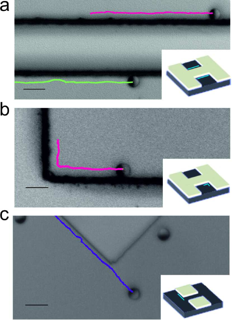
Figure 6: Guidance of Janus microswimmers by step features. (a) A micrograph showing trajectories of two $R=2.5~{}\mathrm{\mu m}$ Janus particles following a straight step (b) A Janus particle tracked while maneuvering around a $90^{\circ}$ corner. (c) A Janus particle unable to follow a reflex angle of $270^{\circ}$. The insets show schematically the structures of wells (a), (b), and posts (c). The blue lines on the insets schematically indicate the position of Janus particles in actual experiments. Scale bars correspond to 10 $\mathrm{\mu m}$.

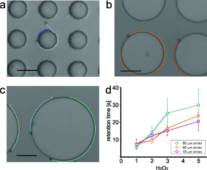
Figure 7: Trapping and guiding active particles by circular posts. (a–c) Optical snapshots of $R=1.0~{}\mathrm{\mu m}$ active particles moving for 12 s around circular posts of 15, 40 and 60 $\mathrm{\mu m}$ diameter $d$, respectively. Scale bar, 20 $\mathrm{\mu m}$. (d) Average retention time as a function of peroxide concentration for $R=1.0~{}\mathrm{\mu m}$. The average is determined for 15 – 20 trajectories per data point; the error bars are standard error of the mean.

This corresponds to particles in a well structure with straight steps. Upon collisions, the particles align along the steps and follow them (Fig. 6a and Supplementary Movie 1). In the same well-like structure, particles eventually encounter a corner and after spending some time adjusting their orientation can maneuver around the corner (Fig. 6b, Supplementary Movie 2). In the case of a post-like structure as displayed in Fig. 6c, particles also follow straight features, but fail to reorient and maneuver around the $270^{\circ}$ corner (see also Supplementary Movie 3). These findings suggest that certain critical value must exist for reflex angles between features above which guidance along the edge of the post is lost.

Active Janus microswimmers also follow circular trajectories around circular posts as shown in Fig. 7, which requires constant reorientation of the axis. In Fig. 7a-c paths are shown where particles with $R=1.0~{}\mathrm{\mu m}$ circle around posts with the diameter of 15, 40 and 60 $\mathrm{\mu m}$, respectively, for more than twelve seconds (see Supplementary Movies 4-6). Supplementary Fig. 3 and Movie 7 show an additional example of cycling motion with long retention times. We find that the retention time of microswimmers at the circular posts increases with increasing peroxide concentration, as displayed in Fig. 7d. At 1% H₂O₂, few particles completely circle around a whole post and in most cases the microswimmers detach from the post before a complete revolution (at lower peroxide concentrations the particles hardly move and get easily stuck at the steps, so measurements were not considered). At 2% H₂O₂ the path length along the posts is increased, and likewise in 3% and 5% H₂O₂, where many particles circle around posts multiple times. At even higher concentrations of H₂O₂, we observe vigorous formation of oxygen bubbles and occurrence of convective flows; thus no reliable measurements could be performed above 5% H₂O₂.

Since the retention time increases with the concentration of H₂O₂, we conclude that it is the activity of the microswimmers which is directly responsible for the effective particle attraction to the posts as well as for the occurrence of the sliding attractor: it is the net result of the particle-step hydrodynamic interaction and confinement induced modification of the distribution of the solute concentration. The strength of both effects depends on the fuel concentration: increased fuel concentration leads to a higher production rate of solute (i.e. stronger phoretic and chemi-osmotic interactions) and a higher self-propulsion velocity (i.e. stronger hydrodynamic interactions). The finite retention time is set by the competition between activity-induced effective attraction to the post side walls and the rotational diffusion. Increased fuel concentration increases the strength of the first factor without affecting the second one, and therefore increases the retention time. The robustness of the sliding state attractor is further discussed in Supplementary Note 5.

III Discussion

We report experimental results showing the dynamics of chemically active Janus microswimmers at geometrically patterned substrates and a qualitative interpretation in terms of a minimal continuum model of self-diffusiophoresis of chemically active colloids. Employing a lithography-based method to fabricate submicron topographic features in the form of rectangular stripes, square posts, cylindrical posts or square wells on glass surface or silicon wafer, we demonstrate that the motion of chemically active Janus microswimmers can be restricted to proceed along these small height patterns for significant time intervals. Furthermore, the motion along the circumference of cylindrical posts reveals that the retention time increases with increasing H₂O₂ concentration. This allows us to unequivocally identify the particle’s chemical activity, which modulates the distribution of the phoretic slip at the particle surface and thus the hydrodynamic interaction with the nearby topography, as playing a dominant role in the observed phenomenology.

We also show that a minimalist, continuum model of self-diffusiophoresis captures the qualitative features of the experimental observations if one accounts for the difference in material properties of the two parts of the colloid, as well as for chemi-osmotic flows induced at the wall. This latter aspect highlights the need for models that explicitly include chemical activity, without which a no-slip boundary condition would apply at the wall. The model employed here allows us to understand the emergence of states of motion along the edges as a simultaneous attraction to two fixed-point attractors corresponding to steady sliding states along the bottom wall and along the vertical wall of the step.

The micro-structuring method presented here avoids the use of any external fields and relies solely on the intrinsic properties of the system to control particle motion. The phenomenology reported here is, in some sense, a mesoscale analogue of the binding of motor-proteins to microtubules to switch to directional motion. However, in distinction to biological nanomotors, the Janus microswimmers bypass the binding and rather elegantly exploit an effective attraction that stems from the feedback between geometric confinement and chemical and hydrodynamic activity. The results presented here open the possibility of robust guidance of particles along complex paths via minimal surface modifications, i.e., by sculpting a pattern with the edge in the desired shape. This may have significant implications in designing new applications based on artificial swimmers. Finally, we consider that these findings will allow further developments by employing smart, chemically patterned walls, where features of the nearby surfaces (and thus the guiding of the microswimmers) can be turned on and off.

IV Methods

IV.1 Sample preparation

Janus particles were obtained by drop casting of a suspension of spherical silica colloids (diameter of 2 or 5 $\mathrm{\mu m}$, Sigma Aldrich) on an oxygen-plasma cleaned glass slide followed by slow evaporation of the solvent and subsequent placement in an e-beam system. High vacuum was applied and subsequently a monolayer of 7 nm Pt was evaporated to guarantee catalytic properties. To release particles from the glass slides into deionized water, short ultrasound pulses were sufficient.

Photoresist patterns were prepared on 24 mm square glass slides or with the same method on silicon wafers. In case of positive photoresist AR-P 3510 was spin-coated onto the cleaned substrate at 3500 rpm for 35 s, followed by a soft bake using a hotplate at 90 ^∘C for 3 min and exposure to UV light with a Mask Aligner (400 nm) for 2 s. Patterns were developed in a 1:1 AR300-35:H₂O solution. In case of negative photoresist a layer of TI prime was spin-coated on the substrate during 20 s at 3500 rpm. After 2 min of drying at 120 ^∘C the negative photoresist was coated employing a program of 35 s spinning at 4500 rpm, followed by 5 min baking at 90 ^∘C. The exposure was carried out with a Mask aligner for 2 s followed by 2 min on the hotplate at 120 ^∘C. Finally an additional exposure to 2 s UV light is applied and the patterns were developed in pure AZ726MIF. The steps were obtained by e-beam deposition the desired material (SiO₂, Si) in the desired thickness. By dissolving the photoresist layer in Acetone the pattern structures of the substrate are exposed, the whole process is illustrated in Supplementary Figure 5.

Prior to experiment the patterned substrates were cleaned by oxygen plasma. Experiments were performed directly on the substrates by adding equal volumes of particles in DI water and diluted peroxide solutions. Videos were recorded with a Leica DFC 300G camera mounted to a Leica upright microscope at approx. 30 fps. Evaluation and tracking was performed using Fiji analysis software.

IV.2 Tracking

Accurate tracking of Janus particles was performed automatically by a specially developed script in Python 2.7 using the OpenCV library. The position of the Janus swimmers at every frame is found by extracting the background, which erases the static posts from the image, leaving only the moving particles.

IV.3 Theoretical Modeling

We model particle motion within a continuum, neutral self-diffusiophoretic framework. A particle emits solute at a constant rate from its catalytic cap. The number density $c(\mathbf{r})$ of solute, where $\mathbf{r}$ is a position in the fluid, is quasi-static. The solute field is governed by the Laplace equation $\nabla^{2}c=0$, and obeys the boundary conditions $-D\nabla c\cdot\mathbf{n}=\kappa$ on the catalytic cap and $-D\nabla c\cdot\mathbf{n}=0$ on the inert face of the particle and the substrate, where $\kappa$ is the rate of emission (uniform over the cap), $D$ is the diffusion coefficient of oxygen, and $\mathbf{n}$ is the local surface normal. Our model neglects the details of the catalytic reaction, which might involve the transport of charged intermediates Golestanian et al. (2005); Golestanian (2009). Nevertheless, we expect this model to capture the gross effects of both near-wall confinement of the solute field and hydrodynamic interaction with nearby walls. The surface gradient of solute drives a surface flow (“slip velocity”) in a thin fluid layer surrounding the particle surface $\mathbf{v}_{s}(\mathbf{r})=-b_{s}(\mathbf{r})\nabla_{||}c$, where $\nabla_{||}$ denotes the projection of the gradient operator along the surface of the particle.

The coefficient $b(\mathbf{r})$ of the slip velocity, the so-called “surface mobility”, is determined by the molecular interaction potential between the solute and the particle surface Anderson (1989). We allow $b(\mathbf{r})$ to differ between the inert and catalytic regions, but assume it is uniform in each region, i.e. take $b_{s}=b_{inert}$ or $b_{s}=b_{cap}$. Additionally, when we consider the effect of chemi-osmotic flow on the substrate, we calculate a wall slip velocity $\mathbf{v}_{w}(\mathbf{r})=-b_{w}\nabla_{||}c$, where $b_{w}$ is a constant. We always take the interaction between the solute and particle surface to be repulsive, i.e. $b_{s}<0$, so that the model is consistent with the observed motion of particles away from their caps.

The velocity $\mathbf{u}(\mathbf{r})$ in the fluid is governed by the Stokes equation $-\nabla p+\nabla^{2}\mathbf{u}=0$ and the incompressibility condition $\nabla\cdot\mathbf{u}=0$, where $p(\mathbf{r})$ is the fluid pressure and $\eta$ is the dynamic viscosity of the solution. The velocity obeys the boundary conditions $\mathbf{u}=\mathbf{v}_{w}(\mathbf{r})$ on the substrate and $\mathbf{u}(\mathbf{r})=\mathbf{U}^{a}+\mathbf{\Omega}^{a}\times(\mathbf{r}-\mathbf{r}_{0})+\mathbf{v}_{s}(\mathbf{r})$ on the particle surface, where $\mathbf{r}_{0}$ is the position of the particle center, and $\mathbf{U}^{a}$ and $\mathbf{\Omega}^{a}$ are the contributions of activity to the translational and rotational velocities of the particle. To obtain $\mathbf{U}^{a}$ and $\mathbf{\Omega}^{a}$ for a given position and orientation of the particle, we first solve for $c(\mathbf{r})$ numerically, using the boundary element method (BEM) Pozrikidis (2002). The slip velocities $\mathbf{v}_{s}$ and $\mathbf{v}_{w}$ are then calculated from $c(\mathbf{r})$. Inserting the slip velocities in the boundary conditions, and requiring that the particle is force and torque free, we solve the Stokes equation numerically via the BEM in order to obtain $\mathbf{U}^{a}$ and $\mathbf{\Omega}^{a}$ in terms of characteristic velocity scales $U_{0}:=|b_{cap}|\kappa/D$ and $\Omega_{0}:=U_{0}/R$. Additionally, $c(\mathbf{r})$ is calculated in terms of a characteristic concentration $c_{0}:=\kappa R/D$.

When we include the effects of gravity, we adopt the geometrical model of Campbell and Ebbens, taking the Janus particle as having a platinum cap that smoothly varies in thickness between a maximum of 7 nm at the pole and zero thickness at the particle equator Campbell and Ebbens (2013). The gravitational contributions to particle velocity, $\mathbf{U}^{g}$ and $\mathbf{\Omega}^{g}$, are calculated using standard methods (see Supplementary Note 1).

We obtain complete particle trajectories by numerically integrating $\mathbf{U}=\mathbf{U}^{a}+\mathbf{U}^{g}$ and $\mathbf{\Omega}=\mathbf{\Omega}^{a}+\mathbf{\Omega}^{g}$. Further details of the numerical method are given in Ref. Uspal et al. (2015). We note that the assumption that the solute field is quasi-static is valid in the limit of small Péclet number $\mathrm{Pe}=U_{0}R/D$. We have neglected the inertia of the fluid, which is valid for small Reynolds number $\mathrm{Re}=\rho U_{0}R/\eta$, where $\rho$ is the mass density of the solution. These dimensionless numbers are $\mathrm{Pe}\approx 4\times 10^{-3}$ and $\mathrm{Re}\approx 10^{-5}$ for a 5 $\mathrm{\mu m}$ catalytic Janus particle that swims at 6 $\mathrm{\mu m~{}s^{-1}}$ Popescu et al. (2010).

Author contributions
S.S. and J.S designed the experiments. J.S. and J.K. performed the experiments and analyzed the data. M.T. and W.E.U. performed numerical calculations. M.N.P. contributed to the theoretical analysis of the numerical results. J.S., W.E.U., and M.T. wrote the manuscript. All the authors discussed the results and commented on the manuscript.

Acknowledgements
The authors thank Albert Miguel Lopez for help with the automated tracking program. W.E.U., M.T., and M.N.P. acknowledge financial support from the DFG, grant no. TA 959/1-1. S.S, J.S and J.K acknowledge the DFG grant no. S.A 2525/1-1. The research also has received funding from the European Research Council under the European Union’s Seventh Framework Programme (FP7/2007-2013)/ERC grant agreement 311529.

Supplementary Information

Supplementary Figures

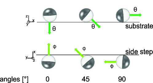
Figure Supplementary Figure 1: Definition of the angles of the microswimmer symmetry axis relative to the substrate and the side step.

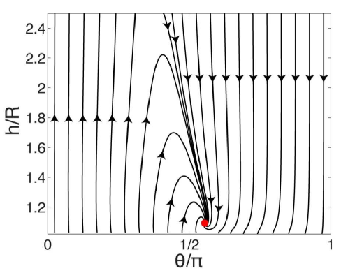
Figure Supplementary Figure 2: Phase portrait for orientation parallel to the substrate of a microswimmer with $R=1.0~{}\mathrm{\mu m}$, including the effect of gravity. Except for the size of the particle, all parameters are the same as in Fig. 2d in the main text.

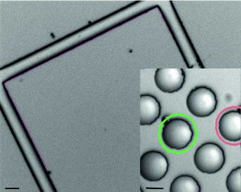
Figure Supplementary Figure 3: $R=2.5~{}\mathrm{\mu m}$ Janus microswimmer trajectories following well features for 227 s; scale bar corresponds to 20 $\mathrm{\mu m}$. Inset: $R=2.5~{}\mathrm{\mu m}$ Janus microswimmer circling around a step for more than 89 s; both tracks were recorded in 5 vol% H₂O₂, scale bar corresponds to 10 $\mathrm{\mu m}$.

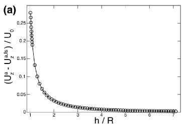
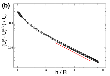
Figure Supplementary Figure 4: Wall-induced change of the particle velocity (a), for a particle with its cap oriented towards the wall ($\theta=0^{\circ}$). Chemi-osmotic and gravitational effects are not included. (b), Same plot as in (a), but with a log-log scale. The red line shows a $(h/R)^{-1}$ scaling.

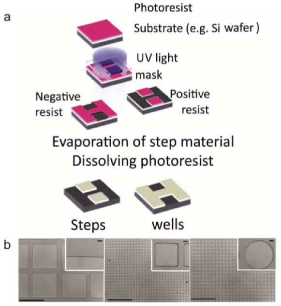
Figure Supplementary Figure 5: Lithography based creation of patterns. (a) Schematic representing the lithography based method to create submicron step and well structures for particle guidance. (b) Optical images of the resulting patterns; the scale bars in the insets correspond to 10 $\mathrm{\mu m}$, while the scale bars in the main images correspond to 500 $\mathrm{\mu m}$.

Supplementary Tables

$B_{2}/B_{1}$	$h_{eq}/R$, no gravity	$\theta_{eq}$, no gravity	$h_{eq}/R$, with gravity	$\theta_{eq}$, with gravity
-7	unstable	unstable	1.16 and 1.04 (backwards)	51.5∘ and 138∘ (backwards)
-5	unstable	unstable	1.19 and 1.03 (backwards)	49.4∘ and 142∘ (backwards)
-3	unstable	unstable	1.26	42.2∘
-1	none	none	1.39	0∘
0	none	none	1.24	0∘
1	none	none	Below 1.02	0∘
3	1.64	102∘	Below 1.02	Around 45∘
5	1.22	114∘	Below 1.02	Around 52∘
7	1.17	117∘	1.032 (backwards)	53.5∘ (backwards)

Table Supplementary Table 1: Attractor states for a squirmer with $R=2.5\;\mathrm{\mu m}$ and $B_{l}=0$ for $l>2$. “Unstable” indicates that there is an unstable fixed point. “None” indicates that there is no fixed point. “Backwards” indicates that the squirmer (which in the bulk swims “away” from the cap) swims towards its cap when in the steady state near the wall, which is not observed experimentally. In some cases (indicated in the table as “Below 1.02”), there are clear signs of an attractor with $h_{eq}/R$ below the numerical cut-off of $h/R=1.02$; however, the corresponding orientations are significantly different from the values $\approx 90^{\circ}$ observed in experiments.

$\beta$	$B_{1}$	$B_{2}$	$B_{3}$	$B_{2}/B_{1}$	$h_{eq}/R$, no gravity	$\theta_{eq}$, no gravity	$h_{eq}/R$, with gravity	$\theta_{eq}$, with gravity
-0.9	0.019	0.413	0.033	22.04	1.05, 1.03 (bwds)	68.9∘, 109∘ (bwds)	1.056, 1.03 (bwds)	66.8∘, 111∘ (bwds)
-0.8	0.038	0.392	0.066	10.44	1.063	69.7∘	1.09	65.3∘
-0.7	0.056	0.370	0.098	6.573	1.075	70.2∘	1.16	59.9∘
-0.6	0.075	0.348	0.131	4.64	1.094	71∘	1.3	48.5∘
-0.5	0.094	0.326	0.164	3.48	$\sim 1.15$ (limit cycle)	$\sim 72^{\circ}$ (limit cycle)	1.56	0∘
-0.4	0.113	0.305	0.197	2.707	unstable	unstable	1.48	0∘
-0.3	0.131	0.283	0.230	2.154	unstable	unstable	1.42	0∘
-0.1	0.169	0.239	0.295	1.418	none	none	1.32	0∘
0	0.188	0.218	0.328	1.16	none	none	1.29	0∘
0.1	0.206	0.196	0.361	0.949	none	none	1.26	0∘
0.3	0.244	0.152	0.427	0.625	none	none	1.21	0∘
0.7	0.319	0.065	0.558	0.205	none	none	1.14	0∘
1.3	0.431	-0.065	0.755	-0.151	none	none	1.09	0∘
2.0	0.563	-0.218	0.984	-0.387	none	none	Below 1.02	0∘

Table Supplementary Table 2: Hydrodynamic properties and attractor locations for the effective squirmer with $R=2.5\;\mathrm{\mu m}$. “Bwds” indicates steady motion towards the cap, which is not observed experimentally. “Limit cycle” indicates one case with a sustained oscillation of small amplitude in $h/R$ and $\theta$. “Unstable” indicates the presence of an unstable fixed point. In one case, there are clear signs of a “hovering” attractor with $h_{eq}/R$ below the numerical cut-off. Although we listed the amplitudes of the first three squirming modes, we note that the effective squirmer can also have $B_{l}\neq 0$ for $l>3$.

Supplementary Note 1: Calculation of Gravitational Contribution to Particle Motion

The particle experiences a gravitational force from the weight of the spherical silica core and platinum cap, as well as a gravitational torque from the bottom-heaviness imparted by the platinum cap. For a given height and orientation of the particle, we use the BEM to calculate the hydrodynamic resistance tensor of the particle. We then obtain the gravitational contributions $\mathbf{U}^{g}$ and $\mathbf{\Omega}^{g}$ to the particle velocity as the product of the inverse of this tensor (i.e. the hydrodynamic mobility tensor) and the vector containing the six components of gravitational force and torque. (Our calculation of the gravitational contribution to velocity therefore includes the effect of hydrodynamic interaction with the planar wall.)

The linearity of the Stokes equation allows one to sum the separate contributions of activity and gravity to determine the complete translational and angular velocities as $\mathbf{U}=\mathbf{U}^{a}+\mathbf{U}^{g}$ and $\mathbf{\Omega}=\mathbf{\Omega}^{a}+\mathbf{\Omega}^{g}$. However, the two sets of velocities must be expressed in the same units. The contributions from particle activity are obtained in terms of $U_{0}:=|b_{cap}|\kappa/D$ and $\Omega_{0}:=U_{0}/R$, i.e., as $\mathbf{U}^{a}/U_{0}$ and $\mathbf{\Omega}/\Omega_{0}$. We estimate $U_{0}$ and $\Omega_{0}$ by taking $U_{p}=6~{}\mathrm{\mu m/s}$ as a typical particle velocity. Within the neutral self-diffusiophoresis framework, $U_{p}/U_{0}$ can be calculated analytically or numerically as a function of the material parameters of the particle, i.e. the extent of catalyst coverage and the spatial variation of surface mobility $b(\mathbf{r})$ [SI1,SI2]. For instance, $U_{p}/U_{0}=1/4$ for half coverage and uniform surface mobility [SI3]. For a given set of material parameters, we can therefore calculate the characteristic velocity $U_{0}$ in dimensional units from $U_{p}/U_{0}$ and $U_{p}=6~{}\mathrm{\mu m/s}$.

Supplementary Note 2: Isolation of contribution to particle motion

We seek to isolate and quantify the various physical contributions to the motion of a particle. We focus on the $x$-component of the angular velocity $\mathbf{\Omega}$. We recall that the linearity of the Stokes equations permits us to solve for active, gravitational, and wall slip (chemi-osmotic) contributions separately and superpose them to obtain the full angular velocity: $\Omega_{x}=\Omega_{x}^{g}+\Omega_{x}^{a}+\Omega_{x}^{ws}$. To obtain the active contribution, we use the Lorentz reciprocal theorem. This theorem allows the problem of determination of $(\mathbf{U}^{a},\mathbf{\Omega}^{a})^{T}$ to be related to six “primed” problems with the same geometry but different boundary conditions. We obtain six coupled equations:

$$\mathbf{U}^{a}\cdot\mathbf{F}^{\prime}_{j}+\mathbf{\Omega}^{a}\cdot\boldsymbol{\tau}^{\prime}_{j}=-\int\limits_{particle}\mathbf{v}_{s}\cdot\boldsymbol{\sigma}^{\prime}_{j}\cdot\mathbf{n}\;dS\;,~{}j=1,\dots,6\;,$$ (1)

where $\mathbf{F}^{\prime}_{j}$ and $\boldsymbol{\tau}^{\prime}_{j}$ are the force and torque, respectively, exerted by quiescent fluid on a particle in steady translation (or rotation) with a no-slip boundary condition on its surface. The index $j$ denotes steady translation in the $\hat{x}$, $\hat{y}$, or $\hat{z}$ direction for $j=1,2,3$, respectively, or steady rotation in $\hat{x}$, $\hat{y}$, or $\hat{z}$ for $j=4,5,6$. Likewise, $\boldsymbol{\sigma}^{\prime}_{j}$ is the fluid stress tensor for the steadily translating or rotating particle. Further details concerning the derivation of Eq. (1) are provided in our previous work [SI4]. We recall that $\mathbf{v}_{s}=-b(\mathbf{r})\nabla_{||}c(\mathbf{r})$. From Eq. (1), we find the component

$$\Omega_{x}^{a}=\sum_{j=1}^{6}(\mathbf{R}^{-1})_{4,j}\int\limits_{particle}b(\mathbf{r})\nabla_{||}c(\mathbf{r})\cdot\boldsymbol{\sigma}^{\prime}_{j}\cdot\mathbf{n}\;dS.$$ (2)

Here, the forces and torques $\mathbf{F}^{\prime}_{j}$ and $\boldsymbol{\tau}^{\prime}_{j}$ have been compactly organized into a matrix $\mathbf{R}$, which has the $k$-th row $\mathbf{R}_{k}$ given by

$$\mathbf{R}_{k}:=\left(\mathbf{F}^{\prime}_{kx},\mathbf{F}^{\prime}_{ky},\mathbf{F}^{\prime}_{kz},\boldsymbol{\tau}^{\prime}_{kx},\boldsymbol{\tau}^{\prime}_{ky},\boldsymbol{\tau}^{\prime}_{kz}\right)\,.$$ (3)

The contribution in Eq. (2) to the angular velocity of the particle is shown in Fig. 3 of the main text.

We now write the activity-induced solute concentration $c(\mathbf{r})=c^{fs}(\mathbf{r})+\delta c(\mathbf{r})$ with a free space component $c^{fs}(\mathbf{r})$ and the wall correction $\delta c(\mathbf{r})$. Similarly, we write $\boldsymbol{\sigma}^{\prime}_{j}=\boldsymbol{\sigma}^{\prime fs}_{j}+\delta\boldsymbol{\sigma}^{\prime}_{j}$ and $\mathbf{R}=\mathbf{R}_{fs}+\delta\mathbf{R}$. Using these representations in the integral in Eq. (2), we may estimate various contributions to the particle rotation.

The free space angular velocity $\Omega_{x}^{a,fs}:=\sum_{j=1}^{6}(\mathbf{R}_{fs}^{-1})_{4,j}\int\limits_{particle}b(\mathbf{r})\nabla_{||}c^{fs}(\mathbf{r})\cdot\boldsymbol{\sigma}_{j}^{\prime fs}\cdot\mathbf{n}\;dS$ is zero, due to the axial symmetry of the particle.

$\Omega_{x}^{a,hi}:=\sum_{j=1}^{6}(\mathbf{R}^{-1})_{4,j}\int\limits_{particle}b(\mathbf{r})\nabla_{||}c^{fs}(\mathbf{r})\cdot\delta\boldsymbol{\sigma}^{\prime}_{j}\cdot\mathbf{n}\;dS$ gives the contribution to $\Omega_{x}^{a}$ strictly from hydrodynamic interactions with the wall. It is plotted in Fig. 3(b) of the main text.

$\Omega_{x}^{a,sol}:=\sum_{j=1}^{6}(\mathbf{R}^{-1}_{fs})_{4,j}\int\limits_{particle}b(\mathbf{r})\nabla_{||}\delta c(\mathbf{r})\cdot\boldsymbol{\sigma}^{\prime fs}_{j}\cdot\mathbf{n}\;dS$ gives the contribution to $\Omega_{x}^{a}$, shown in Fig. 3(c) of the main text, strictly from wall-induced solute modifications. In other words, $\Omega_{x}^{a,sol}$ represents phoretic rotation of the particle from wall-induced concentration gradients. Note that this term is non-zero only when $b_{cap}\neq b_{inert}$; in the case considered here, $b_{inert}/b_{cap}=0.3$.

Finally, the term $\Omega_{x}^{a,\delta\delta}:=\sum_{j=1}^{6}(\mathbf{R}^{-1})_{4,j}\int\limits_{particle}b(\mathbf{r})\nabla_{||}\delta c(\mathbf{r})\cdot\delta\boldsymbol{\sigma}^{\prime}_{j}\cdot\mathbf{n}\;dS$ is due to higher order coupling between the chemical and hydrodynamic effects of the wall. It is depicted in Fig. 3(d) of the main text. Interestingly, it is not necessarily small when the particle is close to the wall.

Now we turn to the other contributions to $\Omega_{x}$. We show the contribution from gravitational torque in Fig. 3(e) of the main text: $\Omega_{x}^{g}\equiv\mathbf{R}^{-1}\mathbf{\mathfrak{F}}^{g}$, where we define a generalized gravitational force $\mathbf{\mathfrak{F}}^{g}\equiv(0,0,F_{z}^{g},\tau_{x}^{g},0,0)^{T}$. This term depends on the size $R$ of the particle; here, it is calculated for $R=2.5\;{\mu m}$.

Likewise, in Fig. 3(f) of the main text, we show the contribution from wall slip, i.e., activity-induced chemio-osmotic flow along the wall: $\Omega_{x}^{ws}\equiv\sum_{j=1}^{6}(\mathbf{R}^{-1})_{4,j}\int\limits_{wall}b_{w}(\mathbf{r})\nabla_{||}c\cdot\boldsymbol{\sigma}^{\prime}_{j}\cdot\mathbf{n}\;dS$. This component is absent in the squirmer model, but it is significant in our case, where $b_{w}/b_{cap}=-0.2$.

Supplementary Note 3: Hydrodynamics-only models

We turn to the wider question of whether the “squirmer” model, in which the interaction with the wall is purely hydrodynamic, can reproduce the experimentally observation for some set of parameters. We recall that the slip velocity of an axisymmetric squirmer can be written as:

$$\mathbf{v}_{s}(\theta_{p})=\sum_{l=1}^{\infty}B_{l}V_{l}(cos(\theta_{p}))\hat{\theta}_{p},$$ (4)

where $\theta_{p}$ is an angle defined with respect to the axis of symmetry, $V_{l}(x)=\frac{2\sqrt{1-x^{2}}}{n(n+1)}\frac{d}{dx}P_{l}(x)$, $P_{l}$ is the Legendre polynomial of order $l$, and $B_{l}$ is the amplitude of squirming mode $l$ [SI5].

An exhaustive search through the squirming mode amplitudes $B_{l}$ is beyond the scope of this work. Nevertheless, we can gain some insight by restricting our consideration to the first two squirming modes. The amplitude of the first mode is set by the free space swimming velocity $v_{f.s.}\approx 6\;\mathrm{\mu m/s}$, since $v_{f.s.}=(2/3)\;B_{1}$. We vary the ratio $B_{2}/B_{1}$, taking $B_{l}=0$ for $l>2$, and determine whether a sliding state emerges (i) in the absence of gravity and (ii) in the presence of gravity, which respectively represent (i) swimming near a side wall, and (ii) swimming above a substrate. The results are shown in Table Supplementary Table 1 for $R=2.5\,\mathrm{\mu m}$. For situation (i), our results show good agreement with Gaffney and Ishimoto [SI5], including the finding that sliding states emerge only for $B_{2}/B_{1}\geq 3$.

We find that, for the parameters considered, the squirmer model cannot reproduce the experimental observation that a particle swims at $\theta\approx 90^{\circ}$ in both situation (i) and situation (ii). Gravity shifts the sliding states that occur for $B_{2}/B_{1}\geq 3$ to $\theta_{eq}\approx 45^{\circ}$. This steady angle would be detectable experimentally as a large apparent coverage of the particles by catalyst. We conclude that, for the parameters considered in Table Supplementary Table 1, the effect of the force dipole (the strength of which is proportional to the amplitude $B_{2}$ of the second squirming mode) is too weak to balance the effect of gravity at $\theta\approx 90^{\circ}$.

In constructing Table Supplementary Table 1, we made two simplifying and physically plausible assumptions: 1.) The contributions of the higher order modes ($l>2$) to the disturbance velocity decay rapidly with distance from the swimmer, and hence contribute negligibly to interaction with the wall; and 2.) the ratio $B_{2}/B_{1}\sim\mathcal{O}(1)$. We can relax both assumptions by considering an “effective squirmer” obtained within our model for a self-diffusiophoretic swimmer. The effective squirmer is obtained for a given $\beta=b_{inert}/b_{cap}$ by neglecting the effect of the wall on the concentration field of a self-diffusiophoretic particle, i.e., by using $c_{f.s.}$ as described in Supplementary Note 2. Additionally, chemi-osmotic effects are neglected. An effective squirmer could have, in principle, non-zero amplitude for all $B_{l}$. Secondly, as shown in Table Supplementary Table 2, the ratio $B_{2}/B_{1}\rightarrow\infty$ as $\beta\rightarrow-1$ from above. This is because, for $\beta\approx-1$, one face of the particle is attracted by solute, and the other repelled by solute; furthermore, the strengths of attraction and repulsion are approximately equal. $B_{1}$ is therefore nearly zero, since it is proportional to the velocity of the particle.

Our results are in Table Supplementary Table 2. We find that, for the parameters studied, the effective squirmer cannot reproduce the experimental observations in both situation (i) and situation (ii). The closest match is for $\beta=-0.8$, with $\theta_{eq}\approx 70^{\circ}$ in situation (i) and $\theta_{eq}\approx 65^{\circ}$ in situation (ii). Achieving this particular sliding state requires a very strong force dipole interaction with the wall: $B_{2}/B_{1}\approx 10$. Is this physically plausible? A recent estimate of the force dipole strength for a catalytic Janus particle was provided by Brown et al. [SI6]. For a $R\approx 1\;\mathrm{\mu m}$ colloid that moves at $U\approx 15\;\mathrm{\mu m/s}$, they estimate $\alpha=30\;\mathrm{\mu m^{3}/s}$. Non-dimensionalizing, and then using the expression from Gaffney and Ishimoto that connects $B_{2}/B_{1}$ with dimensionless $\alpha$ [SI5], we find $B_{2}/B_{1}\approx 2.5$. Hence, the $\beta=-0.8$ effective squirmer is both physically unlikely (having a very large $B_{2}/B_{1}$, i.e., a very large force dipole) and a poorer fit to experimental observations than the full model presented in our work. For more realistic values of the force dipole, hydrodynamics is too weak to, by itself, balance gravitational effects at $\theta\approx 90^{\circ}$.

Supplementary Note 4: Range of interaction with the wall

The interaction of a chemically active particle with a planar wall has a long-ranged character. However, we show that the amplitude (strength) of this interaction is very small except when the particle is close to the wall. This makes it difficult to detect its effects experimentally (at least with the equipment and techniques currently available to us).

In Fig. Supplementary Figure 4(a), we plot the wall-induced change of the wall normal component of the self-diffusiophoretic velocity of a particle that has its cap oriented towards the wall ($\theta=0^{\circ}$). The subtraction of the free space self-diffusiophoretic velocity $U_{z}^{a,fs}=0.1625\,U_{0}$ from $U_{z}^{a}$ isolates the effect of the wall. (Note that chemi-osmotic and gravitational contributions are not included in Fig. Supplementary Figure 4(a).) At $h/R=5$, the contribution to $U_{z}^{a}$ from the wall has already decayed to approximately three percent of the free space self-diffusiophoretic velocity. This change in speed is too small to be apparent when viewing an optical microscopy video of a particle near a step or a side wall. The effect of the wall is even weaker for orientations $\theta>0^{\circ}$.

Our numerical calculations recover the long-ranged character of the interaction. In Fig. Supplementary Figure 4(b), we show the same plot as in (a), but with a log-log scale. Far away from the wall, $\Delta U_{z}^{a}$ follows a $(h/R)^{-2}$ power law, which is shown as a red line. The effect of the wall on the solute field decays as $1/r$, i.e., the leading order term representing the wall is an image point source. Since $\Delta U_{z}^{a}$ is proportional to the wall-induced concentration gradient, it decays as $1/r^{2}$.

Supplementary Note 5: Robustness of the sliding state

Finally, we comment on the robustness of the sliding states against thermal fluctuations, which were not included in our model. To this end we perform a standard linear stability analysis of our dynamical system, which may be written as $\{\dot{h}=f_{1}(h,\theta),\dot{\theta}=f_{2}(h,\theta)\}$, at a fixed point $(h_{eq},\theta_{eq})$ at which $\{f_{1}(h_{eq},\theta_{eq})=0,f_{2}(h_{eq},\theta_{eq})=0\}$. This amounts to determination of the eigenvalues $\lambda_{1,2}$ of the Jacobian matrix $\partial[f_{1},f_{2}]/\partial[h,\theta]$ evaluated at $(h_{eq},\theta_{eq})$.

For the fixed point at Fig. 2d of the main text, we obtain that the Jacobian has eigenvalues $\lambda_{1,2}\simeq(−0.40\pm 0.17\,i)~{}U_{0}/R$. Since the real part of the eigenvalues is negative, the fixed point is a stable attractor: a small perturbation away from the fixed point will exponentially decay with a characteristic timescale $\tau=1/\mathrm{Re}(\lambda_{1})$. To convert this timescale into dimensional units, we use $R=2.5\;\mathrm{\mu m}$ and $U_{0}\approx 6.2~{}U_{f.s.}=6.2\times 6~{}\mathrm{\mu m/s}$, where $U_{f.s.}$ is the self-propulsion velocity of a half-covered Janus swimmer with $b_{inert}/b_{cap}=0.3$ in free space [SI2]. We obtain the timescale $\tau\approx 0.37$ s for the self-trapping of a particle into this sliding state. For comparison, the characteristic timescales of rotational and translational diffusion are $\tau_{r}\approx 97$ s and $\tau_{t}\approx 70$ s, respectively. This separation of timescales indicates that the sliding state in Fig. 2d of the main text is robust against thermal noise. Similarly, for the fixed points in Fig. 2f of the main text and Supplementary Figure 2, we obtain characteristic self-trapping timescales $\tau\approx 1.7$ s $\tau\approx 0.4$ s, respectively (in the latter case we use $R=1.0\;\mathrm{\mu m}$ for the dimensionalization).

SI References

[SI1] Golestanian, R., Phys. Rev. Lett. 102, 188305 (2009).
[SI2] Golestanian, R., Liverpool, T. B., and Ajdari, A., New Journal of Physics 9, 126 (2007).
[SI3] Popescu, M. N., Dietrich, S., and Oshanin, G., J. Chem. Phys. 130, 194702 (2009).
[SI4] Uspal, W. E., Popescu, M. N., Dietrich, S., and Tasinkevych, M., Soft Matter 11, 434 (2015).
[SI5] Ishimoto, K., and Gaffney, E. A., Phys.Rev. E 88, 062702 (2013).
[SI6] Brown, A. T. et al., Soft Matter 12, 131 (2016).

References

- Wang et al. (2013) W. Wang, W. T. Duan, S. Ahmed, T. E. Mallouk, and A. Sen, Nano Today 8, 531 (2013).
- Sánchez et al. (2015) S. Sánchez, L. Soler, and J. Katuri, Angew. Chem., Int.Ed. 54, 1414 (2015).
- Wang (2013) J. Wang, Nanomachines: Fundamentals and Applications (Wiley-VCH, 2013).
- Paxton et al. (2004) W. F. Paxton, K. Kistler, C. Olmeda, A. Sen, S. Angelo, Y. Cao, T. Mallouk, P. Lammert, and V. Crespi, J. Am. Chem. Soc. 126, 13424 (2004).
- Kline et al. (2005) T. R. Kline, W. F. Paxton, T. E. Mallouk, and A. Sen, Angew. Chem., Int. Ed. 44, 744 (2005).
- Fournier-Bidoz et al. (2005) S. Fournier-Bidoz, A. C. Arsenault, I. Manners, and G. A. Ozin, Chem. Commun. , 441 (2005).
- Baraban et al. (2012) L. Baraban, D. Marakov, R. Streubel, I. Moench, D. Grimm, S. Sanchez, and S. O.G, ACS Nano 6, 3383 (2012).
- Hong et al. (2007) Y. Hong, N. M. K. Blackman, N. D. Kopp, A. Sen, and D. Velegol, Phys. Rev. Lett. 99, 178103 (2007).
- Baraban et al. (2013) L. Baraban, H. S. M., S. Sanchez, and O. G. Schmidt, Angew. Chem., Int. Ed. 52, 5552 (2013).
- Dey et al. (2013) K. K. Dey, S. Bhandari, D. Bandyopadhyay, S. Basu, and A. Chattopadhyay, Small 9, 1916 (2013).
- Saha et al. (2014) S. Saha, R. Golestanian, and S. Ramaswamy, Phys. Rev. E 89, 062316 (2014).
- Peng et al. (2015) F. Peng, Y. Tu, J. C. M. van Hest, and D. A. Wilson, Angew. Chem., Int. Ed. 127, 11828 (2015).
- Solovev et al. (2010) A. A. Solovev, S. Sanchez, M. Pumera, Y. F. Mei, and O. G. Schmidt, Adv. Funct. Mater. 20, 2430 (2010).
- Khalil et al. (2013) I. S. M. Khalil, V. Magdanz, S. Sanchez, O. G. Schmidt, and S. Misra, App. Phys. Lett. 103, 172404 (2013).
- Ulbrich et al. (2010) T. C. Ulbrich, C. Bran, D. Marakov, O. Hellwig, J. Risner-Jamtgaart, and D. Yaney, Phys. Rev. B 81, 054421 (2010).
- Albrecht et al. (2005) M. Albrecht, F. Hu, I. Guhl, T. Ulbrich, J. Boneberg, P. Leiderer, and G. Schatz, Nat. Mater. 4, 203 (2005).
- Gunther et al. (2010) C. M. Gunther, O. Hellwig, A. Menzel, B. Pfau, F. Radu, D. Makarov, M. Albrecht, A. Goncharov, T. Schrefl, W. Schlotter, R. Rick, J. Lüning, and S. Eisebitt, Phys. Rev. B 81, 064411 (2010).
- Khalil et al. (2015) I. Khalil, V. Magdanz, S. Sanchez, O. Schmidt, and S. Misra, Int. J. Adv. Robot. Syst. 12, 2 (2015).
- Evans and Lauga (2010) A. A. Evans and E. Lauga, Phys.Rev. E 82, 041915 (2010).
- Spagnolie and Lauga (2012) S. E. Spagnolie and E. Lauga, J. Fluid Mech. 700, 105 (2012).
- Uspal et al. (2015) W. E. Uspal, M. N. Popescu, S. Dietrich, and M. Tasinkevych, Soft Matter 11, 434 (2015).
- Volpe et al. (2011) G. Volpe, I. Buttinoni, D. Vogt, H. J. Kummerer, and C. Bechinger, Soft Matter 7, 8810 (2011).
- Brown et al. (2016) A. T. Brown, I. Vladescu, A. Dawson, T. Vissers, J. Schwarz-Linek, J. Lintuvuori, and W. Poon, Soft Matter 12, 131 (2016).
- Takagi et al. (2016) D. Takagi, J. Palacci, A. Braunschweig, M. Shelley, and J. Zhang, Soft Matter 10, 1784 (2016).
- Spagnolie et al. (2015) S. E. Spagnolie, G. Moreno-Flores, D. Bartolo, and E. Lauga, Soft Matter 11, 396 (2015).
- Palacci et al. (2013) J. Palacci, S. Sacanna, A. Vatchinsky, P. M. Chaikin, and D. J. Pine, J. Am. Chem. Soc. 135, 15978 (2013).
- Howard et al. (1989) J. Howard, A. J. Hudspeth, and R. D. Vale, Nature 342, 154 (1989).
- Howard (2002) J. Howard, Physique des biomolécules et des cellules, edited by F. Flyvbjerg, F. Jülicher, P. Ormos, and F. David, Les Houches - Ecole d’Ete de Physique Theorique, Vol. 75 (Springer Berlin Heidelberg, 2002) pp. 69–94.
- Golestanian et al. (2005) R. Golestanian, T. B. Liverpool, and A. Ajdari, Phys. Rev. Lett. 94, 220801 (2005).
- Golestanian (2009) R. Golestanian, Phys. Rev. Lett. 102, 188305 (2009).
- Anderson (1989) J. L. Anderson, Ann. Rev. Fluid Mech. 21, 61 (1989).
- Pozrikidis (2002) C. Pozrikidis, A Practical Guide to Boundary Element Methods with the Software Library BEMLIB (CRC Press, 2002).
- Campbell and Ebbens (2013) A. I. Campbell and S. J. Ebbens, Langmuir 29, 14066 (2013).
- Popescu et al. (2010) M. N. Popescu, S. Dietrich, M. Tasinkevych, and J. Ralston, Eur. Phys. J. E 31, 351 (2010).