Plasmon-enhanced second harmonic generation in the laser-irradiated cubic metal nanoparticles

Abstract

The plasmon-enhanced second harmonic generation in the subwavelength neutral metal cubic nanoparticles is calculated for the first time in the hydrodynamic and cold plasma approximations. The theory is developed that takes into account all singularities of the electromagnetic field at the cubic nanoparticle surface. The results are compared to the linear case for the nanocube and to those for a spherical nanoparticle. In the latter case, they demonstrate very strong enhancement of the local field strength and the second harmonic signal.

Introduction. – The nonlinear optical properties of subwavelength metal nanoparticles and, in particular, the second harmonic generation are attracting a rapidly growing interest. A lot of effort was directed to the case of spherical and spheroidal nanoparticles, both theoretically Gersten ; Liebsch ; Hayata ; Ostling ; Dewitz ; Dadap1 ; Dadap2 ; Markel ; Huo ; Tomchuk ; Butet2 and experimentally Antoine ; Brevet1 ; ZR ; Viarbitskaya ; Butet1 ; Brevet2 ; Capretti , while much less attention was paid so far to the case of non-spherical nanoparticles, perhaps because of complexity of the problem Neacsu ; Chan ; Zeng ; Scarola ; Gusakov15 . For example, a lot of papers (see FBr and references therein) are devoted to studying linear plasmons in cubic metal nanoparticles, but there is no corresponding investigations of the nonlinear optical properties of cubic nanoparticles and, in particular, the laser induced plasmon-assisted second harmonic generation (SHG). It is worth mentioning a thrust in using high-Z (Sn) plasma EUV and the charged metal particles Krainov02 ; Gusakov15 for high-harmonic generation that may be used in EUV lithography and other applications by way of stripping electrons by laser with their subsequent recapture by the charged ion or the metal particle. Here, we are not interested in multiple ionization regime and will assume that the particles remain neutral at all times. In practice, this corresponds to laser power below some 10 GW/cm² Gusakov15 . The purpose of this work is to investigate the SHG in ideal cubic nanoparticles with free electrons both in far-field and in the near-field and to compare it with the spherical case.

Model. – The basic method for calculating the low order harmonic generation in the subwavelength metal nanoparticles of arbitrary shape was published in Refs. FBr ; FB1 ; FB2 . Using the perturbation theory with respect to the incident laser field FBr ; FB1 ; FB2 , we start from the dimensionless equations for the first-order corrections to the respective quantities defining the alternating electromagnetic field inside the subwavelength neutral metal nanoparticle within the charge compensation approximation (CCA) where the static (zeroth-order) component of the electric field inside the nanoparticle including its narrow boundary vanishes identically ($\mbox{\boldmath$\mathcal{E}$}_{0}\equiv 0$). Introducing the dimensionless coordinates as $\bm{\rho}=\mbox{\boldmath$r$}/a$ with $a$ the cube edge length, and reducing the electron density by dividing it by $z_{i}n_{\mathrm{ion}}$, where $z_{i}$ is the mean ionic charge and $n_{\mathrm{ion}}$ is the reference bulk ion density of the nanoparticle substance, these equations read as

$$\frac{i(\mathscr{N}_{0}-\widetilde{\omega}^{2}-i\gamma\widetilde{\omega})\mbox{\boldmath$\mathcal{E}$}_{1}+i\mathscr{N}_{0}\mbox{\boldmath$\mathcal{E}$}_{L}}{\widetilde{\omega}^{2}+i\gamma\widetilde{\omega}}=\mathrm{curl}\,\mbox{\boldmath$h$}_{1}\,,$$ (1a)

$$\mbox{\boldmath$\mathcal{E}$}_{1}=-\nabla\varphi_{1}\,,\quad\mathrm{div}\,\mbox{\boldmath$h$}_{1}=0\,.$$ (1b)

The expression $\mathscr{N}_{1}=\nabla^{2}\varphi_{1}$ determines the linear correction to the electron density, while $\mathscr{N}_{0}$ defines the static (equilibrium) electron density distribution in the nanoparticle when the laser field is off. Equations (1a)–(1b) are the four first-order differential equations for four quantities, that is for three components of the magnetic vector function $\mbox{\boldmath$h$}_{1}$ and the scalar potential $\varphi_{1}$. In these equations, $\widetilde{\omega}=\omega/\omega_{p}$ is the reduced laser frequency with respect to the bulk plasma frequency $\omega_{p}=\sqrt{4\pi e^{2}z_{i}n_{\mathrm{ion}}/m_{e}}$ with $m_{e}$ and $e$ the electron mass and charge, respectively, $\gamma$ the dimensionless phenomenological damping constant and $\mbox{\boldmath$\mathcal{E}$}_{L}=\mbox{\boldmath$E$}_{L}/E_{0}$ the reduced laser electric field amplitude, with $E_{0}=4\pi ez_{i}n_{\mathrm{ion}}a$. Note that $E_{0}\sim 10^{10}$ V/cm at typical values $z_{i}\sim 1$, $n_{\mathrm{ion}}\sim 10^{22}$ cm^-3 and $a\sim 10$ nm, so in our conditions $\mathcal{E}_{L}$ is always extremely small with respect to unity. All components of the induced electromagnetic field inside the nanoparticle, the harmonic amplitudes $\bm{\mathcal{E}}_{n}$ and $\bm{\mathcal{H}}_{n}$ with $n=1,2\dots$ are normalized by the same way. Besides, magnetic vector function $\mbox{\boldmath$h$}_{n}$ is defined as $\mbox{\boldmath$h$}_{n}=\bm{\mathcal{H}}_{n}/(\omega a/c)$, with $c$ the speed of light and $\omega a/c$ the dipole approximation applicability parameter that should be much less than unity for the subwavelength nanoparticles. In the above equations, the induced magnetic field inside the nanoparticle that enters through the magnetic vector function neither can be eliminated nor neglected, so even in the dipole approximation for subwavelength nanoparticles this can not be reduced to the standard case of the electrostatic approximation.

The case of linear scattering and absorption of the laser field by cubic and parallelepiped-like nanoparticles in the framework of the developed model was considered in detail in Ref. FBr . The solution of the first-order equations should be used as the source term in the second-order equations, which are written as

$$\frac{i(\mathscr{N}_{0}-4\widetilde{\omega}^{2}-2i\gamma\widetilde{\omega})\mbox{\boldmath$\mathcal{E}$}_{2}}{\left(2\widetilde{\omega}^{2}+i\gamma\widetilde{\omega}\right)}=\frac{i\widetilde{\omega}^{2}\mbox{\boldmath$V$}_{2}}{\mathscr{N}_{0}^{{\kern 1.0pt}2}\left(2\widetilde{\omega}^{2}+i\gamma\widetilde{\omega}\right)}+\mathrm{curl}\,\mbox{\boldmath$h$}_{2}\,,$$ (2a)

$$\mbox{\boldmath$\mathcal{E}$}_{2}=-\mbox{\boldmath{$\nabla$}}\varphi_{2}\,,\quad\mathrm{div}\,\mbox{\boldmath$h$}_{2}=0\,,$$ (2b)

with

$$V_{2\alpha}=-\left(-i+\frac{\gamma}{\widetilde{\omega}}\right)2q_{1\alpha}\mathscr{N}_{0}\mathscr{N}_{1}-\mathscr{N}_{0}\frac{\partial(q_{1\alpha}q_{1\beta})}{\partial\rho_{\beta}}$$

$$+q_{1\alpha}q_{1\beta}\frac{\partial\mathscr{N}_{0}}{\partial\rho_{\beta}}-3\frac{\mathcal{E}_{0\alpha}}{\widetilde{\omega}^{2}}\mathscr{N}_{0}\mathscr{N}_{1}^{{\kern 1.0pt}2}-3\frac{\mathcal{E}_{1\alpha}+\mathcal{E}_{{L}{\alpha}}}{\widetilde{\omega}^{2}}\mathscr{N}_{0}^{{\kern 1.0pt}2}\mathscr{N}_{1}$$ (3)

and

$$\mbox{\boldmath$q$}_{1}=\frac{\mathscr{N}_{0}\left(\mbox{\boldmath$\mathcal{E}$}_{1}+\mbox{\boldmath$\mathcal{E}$}_{L}\right)}{i\left(\widetilde{\omega}^{2}+i\gamma\widetilde{\omega}\right)}\,.$$ (4)

Here, the equation $\nabla^{2}\varphi_{2}=\mathscr{N}_{2}$ holds for the second-order correction to the electron density.

Generally, the boundary conditions to these equations read as

$$\frac{1}{4\pi\epsilon_{n}}\oint d\bm{S}^{\prime}\left\{\!\left[\varphi_{n}(\bm{\rho}^{\prime})-\varphi_{n}(\bm{\rho})\right]\frac{\bm{\rho}-\bm{\rho}^{\prime}}{|\bm{\rho}-\bm{\rho}^{\prime}|^{3}}-\frac{\nabla\varphi_{n}(\mbox{\boldmath$\rho$}^{\prime})}{|\bm{\rho}-\bm{\rho}^{\prime}|}\right\}$$

$$=\varphi_{n}(\bm{\rho})-\delta_{1n}\frac{\epsilon_{1}-1}{\epsilon_{1}+2}(\mbox{\boldmath$\mathcal{E}$}_{L}\cdot\bm{\rho})$$ (5)

and

$$\mbox{\boldmath$h$}_{n}(\bm{\rho})+\frac{1}{4\pi}\oint\frac{\left[(\bm{\rho}-\bm{\rho}^{\prime})\times\left[d\bm{S}^{\prime}\times\left(\mbox{\boldmath$h$}_{n}(\bm{\rho}^{\prime})-\mbox{\boldmath$h$}_{n}(\bm{\rho})\right)\right]\right]}{|\bm{\rho}-\bm{\rho}^{\prime}|^{3}}$$

$$-\oint\frac{\left[d\mbox{\boldmath$S$}^{\prime}\times\mathrm{curl}\,\mbox{\boldmath$h$}_{n}(\mbox{\boldmath$\rho$}^{\prime})\right]}{4\pi|\bm{\rho}-\bm{\rho}^{\prime}|}-\frac{1}{4\pi}\!\int\!d^{{\kern 1.0pt}3}\!\rho^{\prime}\left[h_{n\beta}(\bm{\rho}^{\prime})-h_{n\beta}(\bm{\rho})\right]$$

$$\times\frac{3(\rho-\rho^{\prime})_{\alpha}(\rho-\rho^{\prime})_{\beta}-\delta_{\alpha\beta}|\bm{\rho}-\bm{\rho}^{\prime}|^{2}}{|\bm{\rho}-\bm{\rho}^{\prime}|^{5}}=0\,,$$ (6)

where $n$ is the order of nonlinearity and $\epsilon_{n}=\epsilon(n\omega)$ is the dielectric permittivity of the surrounding medium on the $n$th-order laser harmonic frequency. However, in this specific form these boundary conditions are applicable only to the nanoparticles with diffuse surface, when all the quantities including the ion density vary smoothly at the narrow nanoparticle surface. This program was realized for the calculation of the nonlinear properties of metallic spherical nanoparticles in Refs. FB1, ; FB2, . But in the opposite limiting case of the sharp nanoparticle boundary, which we consider here for the cubic nanoparticles, the step-like static electron density $\mathscr{N}_{0}(\mbox{\boldmath$\rho$})$ is equal to one or zero inside or outside the nanoparticle, respectively. In this case, additional boundary conditions following immediately from Eqs. (1a) and (1b) or Eqs. (2a) and (2b), respectively, for $n=1$ or $n=2$ in our case should be taken into consideration to allow for the step-like and higher singularities in the quantities $\nabla\varphi_{n}$ and $\mathrm{curl}\,\mbox{\boldmath$h$}_{n}$ at the sharp nanoparticle surface. In the linear case, it follows from Eqs. (1a) and (1b) that due to steplike discontinuity of the static electron density $\mathscr{N}_{0}$ at the sharp nanoparticle surface, the steplike discontinuities should be also present for some components of $\mbox{\boldmath$\mathcal{E}$}_{1}$ and $\mathrm{curl}\,\mbox{\boldmath$h$}_{1}$, while $\varphi_{1}$ and $\mbox{\boldmath$h$}_{1}$ are themselves continuous. Here, the first-order electron density correction $\mathscr{N}_{1}$ has the $\delta$-function type singularity at the nanoparticle surface. On the other hand, the steplike discontinuities for some components of $\mbox{\boldmath$\mathcal{E}$}_{1}$ and the singularity of $\mathscr{N}_{1}$ generate the $\delta$-function type singularity in function $\mbox{\boldmath$V$}_{\!2}$, which plays the role of the source term in the second-order equations (2a) and (2b). In turn, it generates the $\delta$-function type singularities in some components of $\mbox{\boldmath$\mathcal{E}$}_{2}$ and $\mathrm{curl}\,\mbox{\boldmath$h$}_{2}$, and, as a consequence, the steplike discontinuities in $\varphi_{2}$ and some components of $\mbox{\boldmath$h$}_{2}$. All this should be taken into account in the calculations with the details to be described elsewhere.

The second-order near electric field can be calculated through the second-order electric potential outside the nanoparticle,

$$\varphi_{n}(\bm{\rho})=-\frac{1}{4\pi\epsilon_{n}}\!\int\!d^{{\kern 1.0pt}3}\!\rho^{\prime}\frac{\mathscr{N}_{n}(\bm{\rho}^{\prime})}{|\bm{\rho}-\bm{\rho}^{\prime}|}=-\frac{1}{4\pi\epsilon_{n}}\!\int\!d^{{\kern 1.0pt}3}\!\rho^{\prime}\frac{\nabla^{2}\varphi_{n}(\bm{\rho}^{\prime})}{|\bm{\rho}-\bm{\rho}^{\prime}|}$$

$$=\frac{1}{4\pi\epsilon_{n}}\oint d\bm{S}^{\prime}\left(\varphi_{n}\frac{\bm{\rho}-\bm{\rho}^{\prime}}{|\bm{\rho}-\bm{\rho}^{\prime}|^{3}}-\frac{1}{|\bm{\rho}-\bm{\rho}^{\prime}|}\bm{\nabla}\varphi_{n}\right),$$ (7)

as $\mbox{\boldmath$\mathcal{E}$}_{2}=-\mbox{\boldmath{$\nabla$}}\varphi_{2}$.

For the far-field calculations, the nanoparticle dipole moment for the $n$th-order harmonic can be calculated as

$$d_{n\alpha}=-\int\rho_{\alpha}\,\mathscr{N}_{n}\frac{d^{{\kern 1.0pt}3}\!\rho}{4\pi}=-\int\rho_{\alpha}\,\nabla^{2}\varphi_{n}\frac{d^{{\kern 1.0pt}3}\!\rho}{4\pi}$$

$$=\frac{1}{4\pi}\oint\left\{\varphi_{n}\,dS_{\alpha}-\rho_{\alpha}(d\bm{S}\cdot\bm{\nabla})\varphi_{n}\right\},$$ (8)

where the integration is taken over the outer nanoparticle boundary. The intensity $I_{n}$ of the radiation scattered due to the induced dipole at the $n$th-order harmonic frequency $n\omega$ is defined by the corresponding dipole moment and is given as

$$I_{n}\sim(n\omega)^{4}|\mbox{\boldmath$d$}_{n}|^{2}.$$ (9)

However, it defines both the scattering and the absorbing properties of the cubic nanoparticles only for odd harmonics including the linear case at $n=1$, due to the symmetry properties. For the second harmonic, the dipole scattering intensity vanishes, and it can be used only for testing the calculation code. Thus, for the second-harmonic the scattered intensity is defined by the induced quadrupole moment of the nanoparticle. The dimensionless second-order quadrupole tensor $Q_{2\alpha\beta}$, which is defined in direct analogy with Eq. (8) for the $n$th-order dipole moment, is given by

$$Q_{2\alpha\beta} =-\int(3\rho_{\alpha}\rho_{\beta}-\rho^{2}\delta_{\alpha\beta})\mathscr{N}_{2}\,\frac{d^{{\kern 1.0pt}3}\!\rho}{4\pi}$$

$$=-\int(3\rho_{\alpha}\rho_{\beta}-\rho^{2}\delta_{\alpha\beta})\nabla^{2}\varphi_{2}\,\frac{d^{{\kern 1.0pt}3}\!\rho}{4\pi}$$

$$=\frac{1}{4\pi}\oint\{\varphi_{2}[3\rho_{\alpha}dS_{\beta}+3\rho_{\beta}dS_{\alpha}-2(\bm{\rho}\cdot d\bm{S})\delta_{\alpha\beta}]$$

$$-(3\rho_{\alpha}\rho_{\beta}-\rho^{2}\delta_{\alpha\beta})(d\bm{S}\cdot\bm{\nabla})\varphi_{2}\}\,.$$ (10)

The mean power $P_{2}^{(Q)}$ of quadrupole second-harmonic generation is defined by the dimensionless quadrupole tensor $Q_{2\alpha\beta}$ and is given as

$$P_{2}^{(Q)}\sim(2\omega)^{6}|Q_{2\alpha\beta}|^{2}\,,$$ (11)

with the quadratic dependence on the incident laser wave intensity. The right-hand side of Eq. (11) completely determines the frequency dependence of SHG. The results for these dependencies will be presented next.

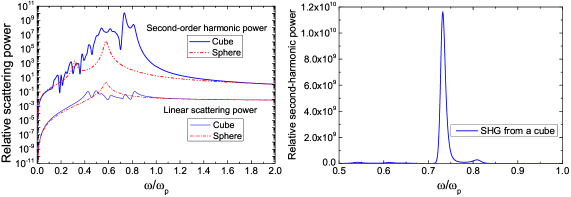
Figure 1: (Color online) The left panel: the laser frequency dependence in the log-scale of the normalized linear scattering power and the second harmonic power for ideal cubic nanoparticle in vacuum (thick and thin solid curves, respectively) as compared with a spherical one of the same volume (dash-double-dotted and dash-dotted curves). The right panel: the frequency dependence of the second harmonic power for the cube in vacuum in the normal scale. For the cube, the electric field amplitude of the incident linear-polarized laser wave is directed along the cube axis perpendicularly to its facets. The damping constant is $\gamma=0.03$.

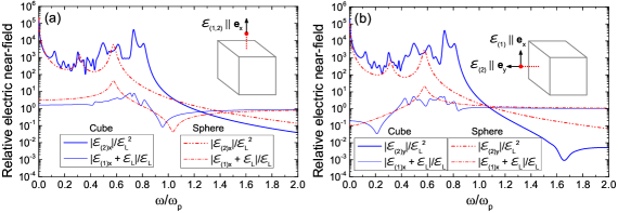
Figure 2: (Color online) The left panel: the laser frequency dependence of the normalized amplitudes of the total electric near-field components corresponding to the linear response and the second harmonic generation for ideal cubic nanoparticle in vacuum (thick and thin solid curves, respectively) just above the center of the top cube face (at $\rho_{x}=0.6$, $\rho_{y}=\rho_{z}=0$) oriented perpendicularly to the laser electric field directed vertically along the $x$-axis, as compared with the same for a spherical nanoparticle of the same volume (dash-double-dotted and dash-dotted curves). The right panel: the same just to the left of the center of the left cube side (at $\rho_{y}=-0.6$, $\rho_{x}=\rho_{z}=0$) oriented in parallel to the laser electric field directed vertically along the $x$-axis. The damping constant is $\gamma=0.03$.

Numerical results. – The calculations for the cubic nanoparticles have been performed on the three-dimensional uniform grid with up to $42\times 42\times 42$ nodal points to get a fair convergence for the second harmonic case, and a good convergence for the linear case, with the whole cube located at $-0.5\leq\rho_{x},\rho_{y},\rho_{z}\leq 0.5$ in the reduced coordinate variables. In this case, the first-order electric potential and three magnetic field components in the cube bulk were given on the cubic grid points themselves, on the vertices of the cubic grid unit cells, while three outside surface electric field components were given on the centers of the cubic grid cell faces on the whole cube surface. All these quantities constitute the complete set of first-order variables, which satisfy a closed set of field equations together with the boundary conditions for a cube. The second-order variables are defined similarly, but in this case the number of variables somewhat increases due to necessity to introduce two sets of the surface variables for the second-order electric potential and some magnetic field components due to their discontinuity on the steplike surface of the nanoparticle.

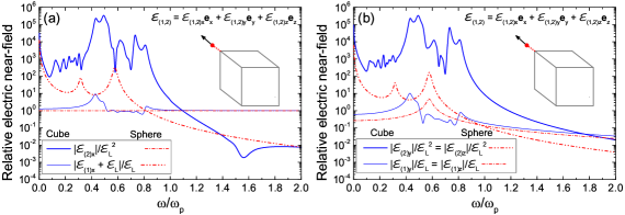
Figure 3: (Color online) The left panel: the laser frequency dependence of the normalized amplitudes of the $x$-component of the total electric near-field corresponding to the linear response and the second harmonic generation for ideal cubic nanoparticle in vacuum (thick and thin solid curves, respectively) just near the vertex of the cube along the cube diagonal (at $\rho_{x}=\rho_{z}=0.558$, $\rho_{y}=-0.558$), with the laser electric field directed vertically along the $x$-axis, as compared with the same for a spherical nanoparticle of the same volume (dash-double-dotted and dash-dotted curves). The right panel: the same for the normalized amplitudes of the $y$- and $z$-components of the total electric near-field corresponding to the linear response and the second harmonic generation, with the laser electric field directed vertically along the $x$-axis. The damping constant is $\gamma=0.03$.

The calculations were performed for both the far-field and the near-field output quantities for the second harmonic. We present the results for the far-field in the vacuum in Fig. 1, while the results for the electric near-field are given in Fig. 2 and Fig. 3. The power of the second harmonic scattered by the nanoparticles versus the laser frequency is presented in the normal scale in the right panel of Fig. 1, with the dominant resonance peak located at $\omega\approx 0.73\omega_{p}$. In the left panel of Fig. 1, we present the detailed structure of the frequency dependence of the scattered second-harmonic power, together with the corresponding results for the linear light scattering by the cubic nanoparticles obtained in the same calculations. Also, the results for both the linear scattering and the second harmonic generation in the spherical nanoparticle of the same volume are shown in this figure for comparison.

First of all, let us note that the asymptotic behavior of the second harmonic power for an ideal cube and for a sphere of the same volume coincide both at low and at high laser frequencies (with respect to the Mie plasmon frequency in a sphere at $\omega/\omega_{p}\approx 0.577$ that corresponds to the strongest peak on the dash-dotted curves). Then, the SHG power in an ideal cube is generally much larger than in a sphere for the mid-range frequencies, especially in the range of the spherical Mie plasmon resonance with a broad maximum on a logarithmic scale shifted to the higher frequencies, where we observe the dominant narrow resonance peak at $\omega\approx 0.73\omega_{p}$. It is in variance with a linear case, where the linear Mie plasmon resonance in a sphere dominates over scattering power in a cube. Note also that the dominant resonance peak in the SHG power in a cube corresponds to some resonance peak in the linear light scattering, which is a relatively weak and does not belong to three largest peaks in the linear light scattering in a cube FBr . On the other hand, the SHG powers in a sphere and in a cube are comparable in the range of the quadrupole resonance in SHG in a sphere that corresponds to the left peak on the dash-double-dotted curve in the left panel of Fig. 1, while it exhibits more complex resonance structure.

We present the results on laser frequency dependence of the normalized (not dependent on the incident laser field) amplitudes of the total electric near-field components corresponding to both the linear response [for $(\bm{\mathcal{E}}_{1}+\bm{\mathcal{E}}_{L})/\mathcal{E}_{L}$] and the second harmonic generation [for $\bm{\mathcal{E}}_{2}/\mathcal{E}_{L}^{2}$] for ideal cubic nanoparticles in vacuum (thick and thin solid curves, respectively, in Figure 2) at the point just above the center of the top cube face (at $\rho_{x}=0.6$, $\rho_{y}=\rho_{z}=0$, the left panel), and just to the left of the center of the left cube side (at $\rho_{y}=-0.6$, $\rho_{x}=\rho_{z}=0$, the right panel). The laser electric field is assumed to be directed vertically, along the $x$-axis. For comparison, similar results for spherical nanoparticles of the same volume (dash-double-dotted and dash-dotted curves) are also presented in both panels of Fig. 2. Note first of all that if in the first case (the left panel of Fig. 2) both the linear response field and the second-harmonic field are directed along the $x$-axis (the direction of the laser electric field), in the second case (the right panel of Fig. 2) the electric field of the second harmonic is directed perpendicular to it and the corresponding cube face, while the linear response field is still parallel to the laser electric field. This fact validates the dipole character of the linear response field and the quadrupole character of the field of the second harmonic. Secondly, note that the laser frequency dependencies of the second harmonic electric field in both cases (the left and the right panels of Fig. 2) are quite similar, with the dominant resonance peak at $\omega\approx 0.73\omega_{p}$, as was the case for the far-field second harmonic power in Fig. 1. Generally, the second harmonic field near the cube is higher than near the sphere although it is not the case for high frequency asymptotic range.

In Figure 3, the laser frequency dependencies of the normalized amplitudes of total electric near-field components corresponding to the linear response and the SHG are presented for ideal cubic nanoparticles in vacuum (thick and thin solid curves, respectively) just near the vertex of the cube along the cube diagonal (at $\rho_{x}=\rho_{z}=0.558$, $\rho_{y}=-0.558$). The laser electric field is directed vertically along the $x$-axis, and the comparison with the same for spherical nanoparticles of the same volume (dash-double-dotted and dash-dotted curves) is given again. The results for the $x$-components are given in the left panel of Fig. 3, while the right panel exhibits the results for $y$- and $z$-components of the total electric near-field corresponding to the linear response and the second harmonic generation. The main difference of this case from the previous one in Fig. 2 is the near-field resonance with two dominant peaks (originating from double-split broad maxima) located at $\omega/\omega_{p}\approx 0.43$ and $\omega/\omega_{p}\approx 0.49$. Note that those peaks are also present in the far-field in Fig. 1 and in the near-field cases, Fig. 2, but they are not dominant. On the other hand, the resonance at $\omega\approx 0.73\omega_{p}$ is also present in the case of Fig. 3, but not as the dominant one. Besides, it should be noted that in this case there is much more noticeable difference between the cube and the sphere with strong increase of the second harmonic field near the cube with respect to that near the sphere of the same volume. It can be connected with the point position near the cube vertex chosen for the results presented in Fig. 3 that can result in the field increasing with respect to the case of sphere with a smooth surface.

Conclusions. – The theory of the laser-assisted second harmonic generation in non-spherical nanoparticles with free electrons was developed and used to calculate the second harmonic both in the far-field and in the near-field versus the laser frequency in subwavelength cubic metal nanoparticles with steplike surface. The results have been compared with the linear response field as well as with the same results for a spherical nanoparticle. They show that the second harmonic in cubic nanoparticles is generally much more intense as compared with the SHG in spherical nanoparticles of the same volume. The dominant resonance frequencies were determined, which for the second harmonic correlate well with those for the linear response case. It is also shown that for the near field the dominant resonance frequencies can be different depending on the position near the nanoparticle.

References

- (1) X. M. Hua and J. I. Gersten, Phys. Rev. B 33, 3756 (1986).
- (2) A. Liebsch, Phys. Rev. Lett. 61, 1233 (1988).
- (3) K. Hayata and M. Koshiba, Phys. Rev. A 46, 6104 (1992).
- (4) D. Östling, P. Stampfli, and K. H. Bennemann, Z. Phys. D 28, 169 (1993).
- (5) J. P. Dewitz, W. Hübner, and K. H. Bennemann, Z. Phys. D 37, 75 (1996).
- (6) J. I. Dadap, J. Shan, K. B. Eisenthal, and T. F. Heinz, Phys. Rev. Lett. 83, 4045 (1999).
- (7) J. I. Dadap, J. Shan, and T. F. Heinz, J. Opt. Soc. Am. B 21, 1328 (2004).
- (8) G. Y. Panasyuk, J. C. Schotland, and V. A. Markel, Phys. Rev. Lett. 100, 047402 (2008).
- (9) B. Huo, X. Wang, S. Chang, M. Zeng, and G. Zhao, J. Opt. Soc. Am. B 28, 2702 (2011).
- (10) P. M. Tomchuk and D. V. Butenko, Ukr. J. Phys. 56, 1110 (2011).
- (11) J. Butet, I. Russier-Antoine, Ch. Jonin, N. Lascoux, E. Benichou, and P.-F. Brevet, J. Opt. Soc. Am. B 29, 2213 (2012).
- (12) R. Antoine, P. F. Brevet, H. H. Girault, D. Bethell, and D. J. Schiffrin, Chem. Commun., 1997, 1901 (1997).
- (13) M. Zavelani-Rossi, M. Celebrano, P. Biagioni, D. Polli, M. Finazzi, L. Duò, G. Cerullo, M. Labardi, M. Allegrini, J. Grand, and P.-M. Adam, Appl. Phys. Lett. 92, 093119 (2008).
- (14) S. Viarbitskaya, V. Kapshai, P. van der Meulen, and T. Hansson, Phys. Rev. A 81, 053850 (2010).
- (15) J. Butet, G. Bachelier, I. Russier-Antoine, C. Jonin, E. Benichou, and P.-F. Brevet, Phys. Rev. Lett. 105, 077401 (2010).
- (16) G. Bachelier, J. Butet, I. Russier-Antoine, C. Jonin, E. Benichou, and P.-F. Brevet, Phys. Rev. B 82, 235403 (2010).
- (17) A. Capretti, E. F. Pecora, C. Forestiere, L. Dal Negro, and G. Miano, Phys. Rev. B 89, 125414 (2014).
- (18) I. Russier-Antoine, E. Benichou, G. Bachelier, C. Jonin, and P.-F. Brevet, J. Phys. Chem. C 111, 9044 (2007).
- (19) C. C. Neacsu, G. A. Reider, and M. B. Raschke, Phys. Rev. B 71, 201402(R) (2005).
- (20) S. W. Chan, R. Barille, J. M. Nunzi, K. H. Tam, Y. H. Leung, W. K. Chan, and A. B. Djurišić, Appl. Phys. B 84, 351 (2006).
- (21) Y. Zeng, W. Hoyer, J. Liu, S. W. Koch, and J. V. Moloney, Phys. Rev. B 79, 235109 (2009).
- (22) M. Scalora, M. A. Vincenti, D. de Ceglia, V. Roppo, M. Centini, N. Akozbek, and M. J. Bloemer, Phys. Rev. A 82, 043828 (2010).
- (23) A. Husakou, S.-J. Im, K.-H. Kim, and J. Herrmann, in Progress in Nonlinear Nano-Optics, edited by S. Sakabe et al., Nano-Optics and Nanophotonics (Springer Intl. Publ. Switzerland, 2015), pp. 251–268.
- (24) S. V. Fomichev and A. M. Bratkovsky, Phys. Rev. B 88, 045433 (2013).
- (25) P. A. C. Jansson, B. A. M. Hansson, O. Hemberg, M. Otendal, A. Holmberg, J. de Groot, and H. M. Hertz, Appl. Phys. Lett. 84, 2256 (2004).
- (26) V. P. Krainov and M. B. Smirnov, Phys. Rep. 370, 237 (2002).
- (27) S. V. Fomichev and W. Becker, Phys. Rev. A 81, 063201 (2010).
- (28) S. V. Fomichev and W. Becker, Contrib. Plasma Phys. 53, 662 (2013).