Advective and diffusive cosmic ray transport in galactic haloes

Abstract

We present 1D cosmic ray transport models, numerically solving equations of pure advection and diffusion for the electrons and calculating synchrotron emission spectra. We find that for exponential halo magnetic field distributions advection leads to approximately exponential radio continuum intensity profiles, whereas diffusion leads to profiles that can be better approximated by a Gaussian function. Accordingly, the vertical radio spectral profiles for advection are approximately linear, whereas for diffusion they are of ‘parabolic’ shape. We compare our models with deep ATCA observations of two edge-on galaxies, NGC 7090 and 7462, at $\lambda\lambda$ 22 and 6 cm. Our result is that the cosmic ray transport in NGC 7090 is advection dominated with $V=150^{+80}_{-30}~{}\rm km\,s^{-1}$, and that the one in NGC 7462 is diffusion dominated with $D=3.0\pm 1.0\times 10^{28}E_{\rm GeV}^{0.5}~{}\rm cm^{2}\,s^{-1}$. NGC 7090 has both a thin and thick radio disc with respective magnetic field scale heights of $h_{\rm B1}=0.8\pm 0.1$ kpc and $h_{\rm B2}=4.7\pm 1.0$ kpc. NGC 7462 has only a thick radio disc with $h_{\rm B2}=3.8\pm 1.0$ kpc. In both galaxies, the magnetic field scale heights are significantly smaller than what estimates from energy equipartition would suggest. A non-negligible fraction of cosmic ray electrons can escape from NGC 7090, so that this galaxy is not an electron calorimeter.

1 Introduction

Following the first detection of a radio halo in an external galaxy by Ekers & Sancisi (1977), it has become clear that radio haloes are ubiquitous among late-type, star forming spiral galaxies (e.g. Hummel et al., 1988; Dahlem et al., 1997; Irwin et al., 1999; Dahlem et al., 2001; Krause et al., 2006; Oosterloo et al., 2007; Heesen et al., 2009a; Soida et al., 2011; Wiegert et al., 2015) and starburst irregular dwarf galaxies (Kepley et al., 2010; Adebahr et al., 2013). Such radio haloes indicate the presence of extra-planar cosmic rays and magnetic fields, because the radio continuum emission in galactic haloes originates predominantly from synchrotron emission of cosmic ray electrons (CRe) spiraling along magnetic field lines. The CRe cooling time-scales are a few $10^{7}$ yr, so that we can infer that they come from the star forming (SF) disc, accelerated and injected by supernovae (SNe). Notably, the radio continuum emission extends in the vertical direction, visible as haloes, but only above star formation sites in the disc plane (Dahlem, Lisenfeld & Rossa, 2006), whereas they hardly extend radially beyond the optical disc (Mulcahy et al., 2014). This has reinforced the view that radio haloes are connected with galactic outflows such as predicted by the ‘Galactic fountain’ model (Shapiro & Field, 1976; Bregman, 1980), where the hot, X-ray emitting gas in superbubbles, heated by multiple SNe, is vented into the halo.

This so-called ‘disc–halo connection’ was first established by the finding that many star-forming galaxies possess a layer of extra-planar diffuse ionized gas (eDIG; Dettmar, 1992; Rossa & Dettmar, 2003a, b). The picture was soon extended to include also the thermal X-ray emission (Tüllmann et al., 2006), a tracer for supernova heated gas. It now has become clear that galaxies also possess extra-planar dust, first seen as sub-mm emission (Neininger & Dumke, 1999) and as absorbing filaments in the optical light (Rossa et al., 2004), meanwhile observed as thermal (far)-infrared emission (Hughes et al., 2014) or as reflected UV-emission (Hodges-Kluck & Bregman, 2014). The thick dusty discs of spiral galaxies are in part produced by the expulsion of dust grains from the thin disc, again showing the existence of a disc–halo connection. It has been noted early on that there is a spatial correlation between the eDIG and the radio continuum emission (Dettmar, 1992). The magnetic field is to very good approximation an ideal MHD plasma and ‘frozen-in’ the ionized gas, although a small amount of resistivity remains, which is in fact essential to facilitate magnetic field amplification by the galactic dynamo. Hence, to first order, in an outflow of ionized gas the magnetic field and cosmic rays are advectively transported together. Vertical gas motions in the disc–halo interface may also open up magnetic field lines, allowing cosmic rays to diffuse along these field lines into the halo. Indeed, magnetic fields in radio haloes have in many cases a significant vertical component. Often, the field lines assume a distinct ‘X’-shaped pattern (e.g. Dahlem et al., 1997; Tüllmann et al., 2000; Krause et al., 2006; Heesen et al., 2009b; Krause, 2009; Soida et al., 2011; Mora & Krause, 2013), which may be caused by a superposition of a plane-parallel and vertical component. Alternatively, the field lines may deviate from the flow lines as expected for a galactic dynamo; although flow lines in hydrodynamical simulations also have a radial component, so that they are neither purely vertical (e.g. Dalla Vecchia & Schaye, 2008).

Table 1: Summary of galaxy parameters.

Parameter	NGC 7090	NGC 7462	Ref.
$D$ (Mpc)	$10.6$	$13.6$	1
Redshift	$0.002825$	$0.003549$	1
Scale (pc $\rm arcsec^{-1})$	51	65	1
Morphological type	Scd	Scd	2
$M_{\rm tot}$ $(10^{10}~{}\rm M_{\sun})$	$0.6$	$0.3$	3
$i$ (from face-on)	$89\degr$	$90\degr$	2
$M_{\rm atom}$ ($10^{9}~{}\rm M_{\sun}$)	$1.73$	$2.37$	2
$V_{\rm rot}$ ($\rm km\,s^{-1}$)	124	112	3
PA	$128\degr$	$73\degr$	4
$S_{\rm 1.4\,GHz}$ (mJy)	$55\pm 3$	$25.6\pm 1.3$	This paper
$S_{\rm th,1.4\,GHz}$ (mJy)	$4.5\pm 0.9$	$1.8\pm 0.9$	$\cdots$
$\rm SFR_{\rm hyb}$ $(\rm M_{\sun}\,yr^{-1})^{*}$	$0.34\pm 0.02$	$0.26\pm 0.05$	$\cdots$
$\rm SFR_{\rm rad}$ $(\rm M_{\sun}\,yr^{-1})$	$0.58\pm 0.03$	$0.43\pm 0.02$	$\cdots$
$\Sigma_{\rm SFR}$ $({\rm M_{\sun}yr^{-1}kpc^{-2}})^{*}$	$1.0\times 10^{-3}$	$7.7\times 10^{-4}$	$\cdots$
$B$ ($\mu\rm G$)	$8.7\pm 1.1$	$8.4\pm 1.1$	$\cdots$
$\alpha$	$-1.06\pm 0.09$	$-1.12\pm 0.09$	$\cdots$
$\alpha_{\rm nt}$	$-1.24\pm 0.11$	$-1.29\pm 0.18$	$\cdots$
$U_{\rm IRF}/U_{\rm B}$	$0.31$	$0.18$	This paper

References – 1: NED Virgo Infall only ($H_{0}=73~{}\rm km\,s^{-1}\,Mpc^{-1}$), 2: Karachentsev et al. (2013), 3: Dahlem et al. (2006), 4: for NGC 7090 determined from $R$-band image, for NGC 7462 from Dahlem, Ehle & Ryder (2001). ^∗ based on hybrid (24 $\mu$m $+$ FUV) SFR

Cosmic rays do not only have the potential to trace outflows, it has been theorized early on that they can be pivotal in driving them, being not subjected to strong radiative losses as the hot, X-ray emitting gas (Ipavich, 1975). A series of papers by D. Breitschwerdt and co-workers (e.g. Breitschwerdt, McKenzie & Völk, 1991, 1993; Dorfi & Breitschwerdt, 2012) have since then laid the theoretical foundation. They found that a cosmic ray driven galactic wind is likely to form. Furthermore, the cosmic rays are able to transfer part of their momentum and energy to the gas thus leading to mass-loaded winds thanks to the coupling between the cosmic rays and the ionized gas, which is usually referred to as the ‘streaming instability’ (Kulsrud & Pearce, 1969). Cosmic ray driven winds remove significant amounts of mass, energy and angular momentum during the evolution of a galaxy. Application to soft X-ray observations of the Milky Way by Everett et al. (2008) has underlined the importance of cosmic rays in launching galactic winds. In their ‘best-fit’ model, the initial wind speed is below the sound speed of the combined thermal and cosmic ray gas (Mach number $M<1)$, accelerates in the halo, where it goes through the critical point ($M$=1) at a distance of 2–3 kpc away from the disc and accelerates further to reach an asymptotic velocity. A consequence of the buoyancy of the relativistic cosmic ray gas is the cosmic ray driven galactic dynamo (Hanasz et al., 2009), where magnetic field lines are stretched and twisted by a combination of cosmic ray buoyancy force, Coriolis force and differential rotation. A galactic wind has profound consequences for the directional symmetry of the magnetic field structure in disc and halo. Moss et al. (2010) could show that mixed parity solutions, e.g. even disc and odd halo parity, can be obtained only if a galactic wind is included in the modelling.

In this paper, we present a radio continuum polarimetry study of two edge-on spiral galaxies, NGC 7090 and NGC 7462, at $\lambda\lambda$ 22 and 6 cm, observed at sub-kpc spatial resolution. We combine our radio observations with Balmer H$\alpha$ emission maps to correct for the contribution of thermal radio continuum emission and use a combination of GALEX FUV and Spitzer and WISE mid-infrared emission to measure spatially resolved star formation rate surface densities ($\Sigma_{\rm SFR}$). Both NGC 7090 and 7462 have been scrutinized in earlier studies. Dahlem, Ehle & Ryder (2001) presented an ATCA radio continuum study at $\lambda\lambda$ 22 and 13 cm, showing that both of them possess radio haloes. In a follow-up study, extending this research to H I observations, Dahlem et al. (2005) showed that both galaxies have thick discs of atomic hydrogen, with irregularities detected both in the H I distribution and velocity field. Furthermore, Rossa & Dettmar (2003a, b) found extra-planar Balmer H$\alpha$ emission, revealing the existence of ionized $H^{+}$ gas in their haloes. Here, we present the re-reduced combined data at $\lambda 22$ cm of Dahlem et al. (2001); Dahlem et al. (2005) with 230 h on-source time and newly acquired observations at $\lambda 6$ cm with 160 h on-source time; we note that we omitted a re-analysis of the $\lambda$13 cm data of Dahlem, Ehle & Ryder (2001), because the observations are less sensitive than either at $\lambda\lambda$ 22 or 6 cm and no further data were acquired. We present also for the first time maps of the linearly polarized radio continuum emission of both galaxies. Some fundamental galaxy parameters are summarized in Table 1.

This paper is organized as follows. In Section 2 we describe our observations and data reduction, followed by Sect. 3, where we describe our analysis of the vertical distribution of the non-thermal radio continuum emission. Our work probes the application of the diffusion–loss equation to describe the transport of cosmic rays as explained in Sect. 4, results of which are presented in Sect. 5. In Sect. 6 we make use of the linear polarization to study the halo magnetic field structure. We discuss implications in Sect. 7 and finish off with a summary of our conclusions in Sect. 8. Throughout the paper, the radio spectral index $\alpha$ is defined in the sense $S_{\nu}\propto\nu^{\alpha}$.

Table 2: ATCA observing journal.

Array	Project ID	Obs Dates	Freq	BWidth	Time
			(MHz)	(MHz)	(h)
—NGC 7090—
750B	C655	1997 Aug 6	$1384.0$	$128.0$	$16.6$
750C	C655	1997 Oct 18	$1384.0$	$128.0$	$15.8$
750A	C655	1998 May 1	$1384.0$	$128.0$	$14.2$
$1.5$D	C655	1998 Oct 16	$1384.0$	$128.0$	$14.0$
$1.5$D	C655	1998 Oct 19	$1384.0$	$128.0$	$6.0$
$1.5$B	C655	1999 Apr 2	$1384.0$	$128.0$	$14.1$
EW352	C1005	2001 Oct 14	$1384.0$	$128.0$	$8.3$
$1.5$D	C1005	2001 Nov 16	$1384.0$	$128.0$	$8.0$
750D	C1005	2003 Feb 23	$1384.0$	$128.0$	$1.4$
750D	C1005	2003 Feb 24	$1384.0$	$128.0$	$8.0$
$1.5$B	C1005	2003 Jan 13	$1384.0$	$128.0$	$8.5$
6D	C1005	2003 Jul 15	$1384.0$	$128.0$	$5.6$
6A	C1005	2003 Dec 13	$1384.0$	$128.0$	$8.6$
$1.5$C	C1487	2005 Nov 29	$4672.0$	$256.0$	$15.8$
6A	C1487	2005 Dec 8	$4672.0$	$256.0$	$15.5$
6A	C1487	2005 Dec 9	$4672.0$	$256.0$	$15.7$
EW352	C1487	2006 Jan 17	$4672.0$	$256.0$	$14.2$
750A	C1487	2006 Jan 22	$4672.0$	$256.0$	$16.4$
—NGC 7462—
750B	C655	1997 Aug 8	$1384.0$	$128.0$	$13.9$
750C	C655	1997 Oct 19	$1384.0$	$128.0$	$13.8$
750A	C655	1998 May 3	$1384.0$	$128.0$	$14.6$
$1.5$D	C655	1998 Oct 18	$1384.0$	$128.0$	$14.8$
$1.5$D	C655	1998 Oct 20	$1384.0$	$128.0$	$1.6$
750D	C1005	2001 Sep 27	$1384.0$	$128.0$	$7.4$
EW352	C1005	2001 Oct 16	$1384.0$	$128.0$	$8.3$
$1.5$D	C1005	2001 Nov 20	$1384.0$	$128.0$	$6.6$
$1.5$B	C1005	2003 Jan 14	$1384.0$	$128.0$	$8.2$
6D	C1005	2003 Jul 16	$1384.0$	$128.0$	$4.8$
6A	C1005	2003 Dec 13	$1384.0$	$128.0$	$8.7$
$1.5$C	C1487	2005 Nov 28	$4672.0$	$256.0$	$15.2$
6A	C1487	2005 Dec 10	$4672.0$	$256.0$	$15.1$
6A	C1487	2005 Dec 11	$4672.0$	$256.0$	$17.7$
EW352	C1487	2005 Jan 15	$4672.0$	$256.0$	$14.2$
750A	C1487	2006 Jan 23	$4672.0$	$256.0$	$16.4$

2 Observations and data reduction

2.1 Radio continuum polarimetry

2.1.1 Observational setup, calibration and imaging

Observations were taken with the Australia Telescope Compact Array (ATCA), prior to the correlator upgrade with its then radio continuum mode. We observed at $\lambda 6$ cm with 2 $\times$ 128 MHz bandwidth distributed in two ‘IFs’ (intermediate frequencies) centered at $4.800$ and $4.544$ GHz, respectively. At $\lambda$22 cm we used a single IF with a bandwidth of $128$ MHz centered at $1.384$ GHz, where the other IF was used either for a simultaneous observing of continuum emission at $\lambda$13 cm (project code C655) or for observing of the H I line of atomic hydrogen (C1005). Observing runs lasted typically 10 h, or longer, to ensure good (u,v)-coverage, and started with a 10–15 min long scan of J1938$-$634 as flux (primary) calibrator, which is also used to measure the absolute polarization angle. Observations of our source were interleaved every 30 min with a 5 min observation of a phase (secondary) calibrator, which were J2106$-$413 and J2117$-$642 for NGC 7090 and 7462, respectively. Each observing run had enough parallactic angle coverage ($\goa 60\degr$), so that we were able to calibrate for the instrumental polarization of all antennae. The ATCA is an East–West interferometer, consisting of six 22-m antennae, five of which (CA01–CA05) are movable along a railway track. We used a variety of configurations ranging from the compact EW352 (350-m maximum baseline) to the extended 6A ($2.9$-km maximum baseline) configuration in order to fill in the (u,v)-plane with visibilities, so that we are sensitive to extended emission. A journal of the observations is presented in Table 2.

We followed standard data reduction procedures using MIRIAD (Sault, Teuben & Wright, 1995), setting our flux densities according to the Baars et al. (1977) flux scale. For imaging, we used the Multi-Scale Multi-Frequency Synthesis (MS–MFS) cleaning algorithm (Rau & Cornwell, 2011) of the Common Astronomy Software Applications (CASA; McMullin et al., 2007). MS–MFS cleaning removes any residual flux densities very efficiently (Hunter et al., 2012), which is particularly important for extended sources that are large in comparison to the synthesized beam. We inverted the (u,v)-data where we used a ‘Briggs’ robust weighting of $0.5$ in total power radio continuum (Stokes $I$) and an outer (u,v)-taper of $12\times 24~{}\rm k\lambda$ ($\rm PA=90\degr$) in order to boost the signal-to-noise ratio (S/N). Antenna CA06 is at a fixed location, approximately 3 km away from the nearest of the other antennae. Including it results in having baselines up to 6 km length, whereas without it the baseline lengths are smaller than 3 km. Hence, we included antenna CA06 for the $\lambda 22$ cm maps, but not in the $\lambda 6$ cm maps, resulting in a similar (u,v)-coverage and angular resolution. We used cleaning scales of up to 300 arcsec angular size, similar to the angular extent of our galaxies, and we cleaned all maps until we reached components with amplitudes of 2 $\times$ the rms noise level. For the maps in polarization (Stokes $Q$ and $U$) we used natural weighting and left out antenna CA06 both at $\lambda\lambda$ 22 and 6 cm, in order to boost the sensitivity of weak extended emission. Because our synthesized beam in polarization was relatively large (27–34 arcsec) and the emission in Stokes $Q$ and $U$ is relatively compact, we chose to clean the maps with the MFS implementation of clean in MIRIAD, without the use of multiple angular cleaning scales.

2.1.2 Specific data reduction issues

We encountered several specific issues with our data, which required a special treatment, which we outline in the following. Firstly, the wide field-of-view (FoV) of the $\lambda 22$ cm maps meant that a number of bright sources, mostly unresolved, were in the outskirts of the map close to the half-power point or beyond. Because of the uncertainty of the primary beam model in this region, and the fact that small positional changes (phase errors) will result in large changes of the antenna amplitude gains, sources can have significant residual sidelobes after cleaning, increasing the rms noise level of the maps. Hence, we attempted to ‘peel’ the sources away, by tailoring antenna gain solutions to them and subsequently subtracting them from the (u,v)-data. We applied the following procedure: firstly, we subtracted all sources in the field except the source to be peeled from the (u,v)-data using clean components. Then a self-calibration in amplitude and phase (GAINCAL in CASA with a 600 s solution interval) was performed using a model of the to be peeled source only, resulting in amplitude and gain corrections to the antennas. The model of the source was inserted into the model column of the measurement set with FT in CASA and the gain corrections were applied to this model column using the CASA toolkit function CB.CORRUPT. The source was subtracted with UVSUB. The map was cleaned again in order to create an updated model of the field and the procedure was repeated with the next source to be peeled. We subtracted eight sources from each map in this way, where we grouped several unresolved sources together if they were nearby to each other. As the last step, we performed two rounds of ordinary self-calibration in phase only on the entire field, using a solution interval of 200 s. In this way we were able to remove the sidelobes of the bright sources in a sufficient way, leading to an improved rms noise level, 25 per cent lower than in the un-peeled maps. We checked that the flux densities of our galaxies changed by only 3 per cent at most.

Table 3: Total power (TP) and polarized intensity (PI) maps.

Galaxy	$\lambda$	Resolution (arcsec)		Noise ($\rm\mu Jy\,beam^{-1}$)
	(cm)	TP	PI	$\sigma_{\rm TP}$	$\sigma_{\rm PI}$
NGC 7090	22	$13.8$	$30.4$	28	27
NGC 7090	6	$13.8$	$27.5$	13	12
NGC 7462	22	$13.9$	$37.4$	25	26
NGC 7462	6	$13.9$	$27.0$	9	12

Another issue we encountered was that we were not able to use the first five channels (of the 13 channels in total) at $\lambda$22 cm in polarization, because ring-like structures appeared in the maps that could not be identified and flagged in the (u,v)-data. It should be noted that channel number three was flagged by the online flagging system, and the adjacent channels (two and four) showed the strongest ring-like structures, so that the problem was obviously in the data recording and not some transient radio frequency interference (RFI) affecting the data, which we could have flagged. Lastly, we note that the largest angular structure the ATCA can image well at $\lambda$6 cm in the EW352 array is 460 arcsec, assuming an observing time of 1 d. Both our galaxies fall comfortably within this limit, with the largest angular scale of 300 arcsec, as estimated from the star formation rate surface density maps (Figs 1(b) and 2(b)).

All maps were primary beam corrected using LINMOS (part of MIRIAD), before we exported them into FITS format and took them for further analysis into AIPS. Details of the maps presented in this paper can be found in Table 3, where angular resolutions are referred to as the full-width at half-mean (FWHM).

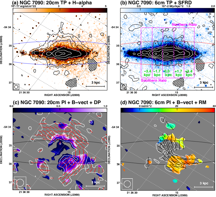
Figure 1: ATCA observations of NGC 7090. Top left: $\lambda$22 cm total power (TP) radio continuum emission at $13.8$ arcsec resolution overlaid on a Balmer H$\alpha$ emission map, convolved with a 3 arcsec Gaussian kernel to highlight weak, diffuse emission. Contours are at 3, 6, 10, 20, 40 and 80 $\times$ 28 $\rm\mu Jy\,beam^{-1}$. Hatched areas show masked map regions. Top right: $\lambda$6 cm total power (TP) radio continuum emission at $13.8$ arcsec resolution, overlaid on a $\Sigma_{\rm SFR}$ map ($\rm FWHM=6.7~{}arcsec$) from a linear combination of GALEX FUV and Spitzer 24 $\mu$m emission. Contours are at $-3$, 3, 6, 10, 20, 40, and 80 $\times$ 13 $\rm\mu Jy\,beam^{-1}$. Hatched areas show masked map regions. The stripes used for measuring the non-thermal radio continuum scale heights are shown as well. Bottom left: $\lambda$22 cm linearly polarized intensity (PI) and $B$-vectors at $30.4$ arcsec resolution, overlaid on the degree of depolarization (DP) between $\lambda\lambda$ 22 and 6 cm (0: entirely depolarized, 1: no depolarization, $\sigma_{\rm DP}=0.3$), where a constant non-thermal radio spectral index of $-1.26$ was assumed. Contours are at 2, 4, and 6 $\times$ 27 $\rm\mu Jy\,beam^{-1}$. Bottom right: $\lambda$6 cm linearly polarized intensity (PI) and $B$-vectors at $27.0$ arcsec resolution, overlaid on the rotation measure (RM) between $\lambda\lambda$ 22 and 6 cm ($\sigma_{\rm RM}=10~{}\rm rad\,m^{-2})$. Contours are at 2, 4, and 6 $\times$ 12 $\rm\mu Jy\,beam^{-1}$. $B$-vectors are of polarized emission: the position angle of the polarized electric field rotated by $90\degr$, not corrected for Faraday rotation, with the length proportional to the polarized intensity and only plotted where $\rm PI\geq 2\sigma_{PI}$. Ellipses show the optical extent of the disc ($7.4\times 1.3$ arcmin, source: NED). The maps were rotated, so that the major axis is aligned in East–West orientation.

Figure 2: ATCA observations of NGC 7462. Top left: $\lambda$22 cm total power (TP) radio continuum emission at $13.9$ arcsec resolution overlaid on a Balmer H$\alpha$ emission map, convolved with a 3 arcsec Gaussian kernel to highlight weak, diffuse H$\alpha$ emission. Contours are at $-3$, 3, 6, 10, 20, 40 and 80 $\times$ 25 $\rm\mu Jy\,beam^{-1}$. Hatched areas show masked map regions. Top right: $\lambda$6 cm total power (TP) radio continuum emission at $13.9$ arcsec resolution, overlaid on a $\Sigma_{\rm SFR}$ map ($\rm FWHM=12~{}arcsec$) from a linear combination of GALEX FUV and WISE 22 $\mu$m emission. Contours are at $-2$, 2, 4, 8, 16, 32, and 64 $\times$ 9 $\rm\mu Jy\,beam^{-1}$. Hatched areas show masked map regions. The stripes used for measuring the non-thermal radio continuum scale heights are shown as well. Bottom left: $\lambda$22 cm linearly polarized intensity (PI) and $B$-vectors at $37.4$ arcsec resolution, overlaid on the degree of depolarization (DP) between $\lambda\lambda$ 22 and 6 cm (0: entirely depolarized, 1: no depolarization, $\sigma_{\rm DP}=0.3$), where a constant non-thermal radio spectral index of $-1.26$ was assumed. Contours are at 2, 4, and 6 $\times$ 26 $\rm\mu Jy\,beam^{-1}$. Bottom right: $\lambda$6 cm linearly polarized intensity (PI) and $B$-vectors at $27.0$ arcsec resolution, overlaid on the rotation measure (RM) between $\lambda\lambda$ 22 and 6 cm ($\sigma_{\rm RM}=10~{}\rm rad\,m^{-2})$. Contours are at 2 and 4 $\times$ 12 $\rm\mu Jy\,beam^{-1}$. $B$-vectors are of polarized emission: the position angle of the polarized electric field rotated by $90\degr$, not corrected for Faraday rotation, with the length proportional to the polarized intensity and only plotted where $\rm PI\geq 2\sigma_{PI}$. Ellipses show the optical extent of the disc ($4.6\times 1.2$ arcmin, source: DSS blue). The maps were rotated, so that the major axis is aligned in East–West orientation.

2.2 Thermal radio continuum emission

We created maps of the thermal (free–free) radio continuum emission using Balmer H$\alpha$ emission line maps following standard conversion (e.g. Deeg, Duric & Brinks, 1997, equation 3, electron temperature $T=10^{4}$ K). NGC 7090 is part of the Local Volume Legacy (LVL) survey (Kennicutt et al., 2008), where calibrated H$\alpha$ and continuum subtracted H$\alpha$ maps are readily available. NGC 7090 and 7462 are part of the H$\alpha$ survey by Rossa & Dettmar (2003a, b), who supplied us with un-calibrated, but continuum subtracted H$\alpha$ and an $R$-band optical maps. In order to bootstrap the H$\alpha$ flux of NGC 7462, we assumed that the ratio of the H$\alpha$ to the $R$-band flux is identical for both NGC 7090 and 7462 in instrumental units. We obtained $R$-band fluxes from Doyle et al. (2005) and scaled the H$\alpha$ map of NGC 7462 accordingly. We estimate the accuracy of this method to be accurate within 50 per cent. This is, however, for the purpose of this work accurate enough. At a reference height of 2 kpc, the thermal radio continuum fraction is only 5 per cent at $\lambda 6$ cm in NGC 7462. Hence, even a 50 per cent uncertainty will hardly change the results of our scale height analysis.

Foreground stars in the H$\alpha$ maps were masked, and pixels replaced with values of surrounding pixels. NGC 7462 was surrounded by a bowl of negative emission, probably due to a too conservative continuum subtraction. We corrected this using a constant offset, where all emission outside of the bowl was blanked. All data were corrected for foreground absorption, using $A_{V}=2.5\times E(B-V)~{}\rm mag$, where we used the $E(B-V)$ magnitudes from Schlafly & Finkbeiner (2011). We did not correct for internal absorption due to dust in the galaxies, which means that we may underestimate the amount of thermal radio continuum emission, particularly in the disc plane. We will come to this limitation in the following analysis and discuss its implications there (Sects 5.2 and 5.3).

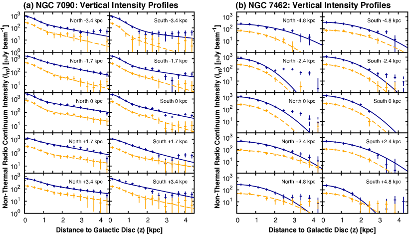
Figure 3: Vertical profiles of the non-thermal radio continuum intensity as function of the distance to the galactic midplane. The offset of each stripe centre is indicated in each panel where ‘$+$’ indicates an offset to the East and ‘$-$’ to the West (see Figs 1(b) and 2(b)). Data points denote the average radio continuum intensity at $\lambda\lambda$ 22 and 6 cm. Lines indicate least-squares fits to the data points, where solid, dark-blue lines are fits to the $\lambda$22 cm data points and dashed, orange lines to those at $\lambda$6 cm. Left: NGC 7090, where the fits are two-component exponential functions. Right: NGC 7462, where the fits are one-component Gaussian functions. Three stripes at $\lambda$22 cm ($-2.4$ kpc North and South, 0 kpc North) show halo emission as a second, more extended, component (see text).

3 Analysis

We present the radio continuum maps of NGC 7090 and 7462 in Figs 1 and 2, respectively. Both galaxies clearly display extra-planar radio continuum emission, extending beyond the optical disc, which we will analyse in this section. Before we proceed, we subtract the thermal radio continuum (free–free) emission using Balmer H$\alpha$ as a tracer, so that we are left over with the non-thermal radio continuum emission only. Furthermore, we have masked unrelated background sources, which are mostly point-like, i.e. unresolved. The exception is an area in the southern halo of NGC 7462, centred on $\rm J2000.0$ RA $23^{\rm h}02^{\rm m}48\aas@@fstack{s}3$ Dec. $-40\degr 51\arcmin 12\arcsec$, which contains diffuse emission. It also harbours one double-peaked ($65~{}\rm\mu Jy$ each) background source at RA $23^{\rm h}02^{\rm m}48\aas@@fstack{s}7$ Dec. $-40\degr 50\arcmin 48\arcsec$, with 3 arcsec separation ($\rm PA\approx 240\degr$), which we could split with the full resolution (6-km baseline) $\lambda$6 cm observations. Because the emission in this area is morphologically very different from the remaining radio continuum emission, and clearly separated, we masked it as unrelated background emission. It may be speculated that the masked spurious emission is related to an active galactic nucleus (AGN); but we did not find any prominent unresolved source ($>$$70~{}\rm\mu Jy$) in the centre of NGC 7462, which would hint at any past or current AGN activity.

3.1 Non-thermal radio continuum emission

3.1.1 Scale heights

Following Dumke et al. (1995), we used analytical functions that allow the fitting of vertical radio continuum emission profiles with one or two component Gaussian or exponential functions, where the instrumental point spread function (PSF) is assumed to be of Gaussian shape. In addition to the PSF, a correction for projected disc emission can be added, for instance by fitting a Gaussian and adding the FWHM in quadrature. Assuming that both of our galaxies are in an almost exact edge-on position ($i\geq 89\degr$), no such correction is required. Hence, we use an effective beam size $\sigma=0.5\cdot{\rm FWHM}/\sqrt{2\ln(2)}\approx 0.425\cdot{\rm FWHM}$, where FWHM is the angular (spatial) resolution of our maps, resulting in $\sigma=0.30$ and $0.38$ kpc for NGC 7090 and 7462, respectively. As we shall see, in our case a one-component Gaussian function is appropriate for one of our galaxies, for which the analytical function is:

$$W_{\rm Gauss}(z)=\frac{w_{o}z_{0}}{\sqrt{2\sigma^{2}+z_{0}^{2}}}\exp\left(-\frac{z^{2}}{2\sigma^{2}+z_{0}^{2}}\right),$$ (1)

with $\sigma$ being the effective beam size, $w_{0}$ the maximum of the distribution and $z_{0}$ the (Gaussian) scale height. For the second galaxy in our study, a two-component function is appropriate, of which one component takes the following form:

$$W_{\rm exp}(z) = \frac{w_{0}}{2}\exp\left(-\frac{z^{2}}{2\sigma^{2}}\right)$$ (2)

$$\times\left[\exp\left(\frac{\sigma^{2}-zz_{0}}{\sqrt{2}\sigma z_{0}}\right)^{2}{\rm erfc}\left(\frac{\sigma^{2}-zz_{0}}{\sqrt{2}\sigma z_{0}}\right)\right.$$

$$\left.+\exp\left(\frac{\sigma^{2}+zz_{0}}{\sqrt{2}\sigma z_{0}}\right)^{2}{\rm erfc}\left(\frac{\sigma^{2}+zz_{0}}{\sqrt{2}\sigma z_{0}}\right)\right],$$

with the complementary error function:

$${\rm erfc}(x)=1-{\rm erf}(x)=\frac{2}{\sqrt{\pi}}\int_{0}^{\infty}\exp(-r^{2}){\rm d}r.$$ (3)

Again, $\sigma$ is the effective beam size, $w_{0}$ the maximum of the distribution and $z_{0}$ the (exponential) scale height. We averaged the maps in stripes in order to raise the S/N of the weak emission in the halo. A stripe width around 2 kpc is ideal to do this, because this is the maximum typical diffusion length of cosmic rays in the disc (Murphy et al., 2008; Tabatabaei et al., 2013b), so that we do not smear out a change of the local scale height. Hence, we used widths of $1.7$ kpc (NGC 7090) and $2.4$ kpc (NGC 7462), sampled with a vertical spacing of 7 arcsec, which is half of our angular resolution, equivalent to 350 and 460 pc in NGC 7090 and 7462, respectively. The stripes for the extraction of the vertical profiles are shown in Figs 1(b) and 2(b); these were fitted using a least-squares routine, which provides a formal error of the fit parameters. The profiles along with the fits are presented in Fig. 3 and averaged scale heights are tabulated in Table 4 (see Appendix B for the scale heights in the individual stripes).

We find that in NGC 7090 the vertical profiles can be equally well described by a two-component exponential ($\chi^{2}=1.3$) or a two-component Gaussian fit ($\chi^{2}=1.2$). Presented in Fig. 3(a) are the exponential fits, because, as we shall see in Sect. 5, the advective transport of cosmic rays in NGC 7090 favours them over Gaussian profiles. The thin disc in NGC 7090 has non-thermal scale heights of $0.35\pm 0.06$ and $0.37\pm 0.08$ kpc ($\lambda\lambda$ 22 and 6 cm) in the northern and $0.40\pm 0.06$ and $0.29\pm 0.10$ kpc in the southern thin disc. In NGC 7462, the profiles shown in Fig. 3(b) can be better fitted with a one-component Gaussian fit ($\chi^{2}=0.6$) than by a one-component exponential fit ($\chi^{2}=1.5$), except at $\lambda$22 cm in the northern halo, where the one-component exponential fit is better ($\chi^{2}=1.2$) than a one-component Gaussian fit ($\chi^{2}=2.7$). This is largely because of a second, more extended component, which can be traced in the northern stripes at offsets of $-2.4$ and 0 kpc; a similar, albeit less prominent, component can be found in the southern stripe at an offset of $-2.4$ kpc. Because we do not detect this emission in any of the other stripes, nor at $\lambda$6 cm, we omit it in the following analysis.

Notably, NGC 7462 does not have a thin disc. The only other galaxy known to have a Gaussian vertical profile is NGC 4594 (M104, the Sombrero Galaxy), an Sa galaxy, which is dominated by its large central bulge (Krause, Wielebinski & Dumke, 2006). However, we have to caution that this result can be changed when also fitting for the baselevel. A baselevel of $\approx$$-1\sigma_{\rm TP}$ allows us to fit the profiles with an exponential function with a similar reduced $\chi^{2}$ as for the Gaussian fit. We will come back to the significance of this finding in the further analysis of NGC 7462 (Sect. 5.3). If we were to fit the profiles with a one-component exponential function, the scale height would be only $0.9\pm 0.1$ kpc, both at $\lambda\lambda$ 22 and 6 cm, significantly less than in NGC 7090 and observed in other galaxies (Krause, 2011), underlining that the radio halo of NGC 7462 is different from that of most other galaxies.

It should be noted that the inclination angles we used were derived from the ratio of the optical minor to major axis, so that they are not very reliable. But we found that for an inclination angle of $i=85\degr$ the scale height of the thick disc for both a one-component Gaussian or a two-component exponential fit decreases by two per cent only. Hence, we conclude that our scale height measurements are robust with respect to the uncertainty of the inclination angle.

Table 4: Non-thermal radio continuum scale heights $z_{0}$.

Galaxy	$\lambda$	North	South	Weighted mean
	(cm)	(kpc)	(kpc)	(kpc)
NGC 7090	22	$1.73\pm 0.17$	$1.53\pm 0.39$	$1.70\pm 0.22$
NGC 7090	6	$1.90\pm 0.69$	$1.14\pm 0.44$	$1.35\pm 0.51$
NGC 7462	22	$1.57\pm 0.10$	$1.44\pm 0.05$	$1.47\pm 0.06$
NGC 7462	6	$1.31\pm 0.07$	$1.39\pm 0.04$	$1.36\pm 0.05$

Notes – Values are weighted arithmetic means of the scale heights measured in the stripes. Scale heights in NGC 7090 are referring to the thick disc from the two-component exponential fitting functions; in NGC 7462 they refer to the disc from the one-component Gaussian fitting functions.

3.1.2 Radio spectral index

The galaxy-wide integrated radio spectral indices for both galaxies are $\approx$$-1.1$ and $\approx$$-1.3$, for the total and non-thermal radio continuum emission, respectively. The steep non-thermal spectral index indicates that in both galaxies CRe radiation losses, synchrotron and inverse Compton radiation, are important and the CRe escape fraction is small (Lisenfeld & Völk, 2000). Hence, as a second characterization of the vertical distribution of the non-thermal radio continuum emission, we measure profiles of the non-thermal radio spectral index. The radio continuum emission in the halo is weak, adversely affecting the accuracy of spectral index measurements. A higher S/N value reduces the uncertainty, so that we averaged only in one stripe between the same offsets along the major axis as used for measuring the scale heights ($\pm 4.25$ kpc for NGC 7090, $\pm 6.0$ kpc for NGC 7462). We present the vertical profiles of the non-thermal radio spectral index in Fig. 4 (these values can be found in Appendix B).

In NGC 7090, the non-thermal radio spectral index is $-1.0$ in the galactic midplane and steepens rapidly to $-1.4\leq\alpha_{\rm nt}\leq-1.2$ within heights of 2 kpc. From then on, the radio spectral index steepens less rapidly reaching values of $\approx$$-1.5$ at a height of 4 kpc, the limit to which we can measure its value with a sufficient degree of certainty. In contrast, the radio spectral index in NGC 7462 shows only little steepening within heights of 2 kpc, where values of $-1.3\leq\alpha_{\rm nt}\leq-1.2$ are found. At heights larger than 2 kpc, however, the spectral index steepens rapidly, particularly in the northern halo, reaching there a value of $-2.2\pm 0.4$. In Sect. 4 we will present idealized models for the transport of cosmic rays, in order to calculate synthetic spectral index profiles, which we can compare with the observations.

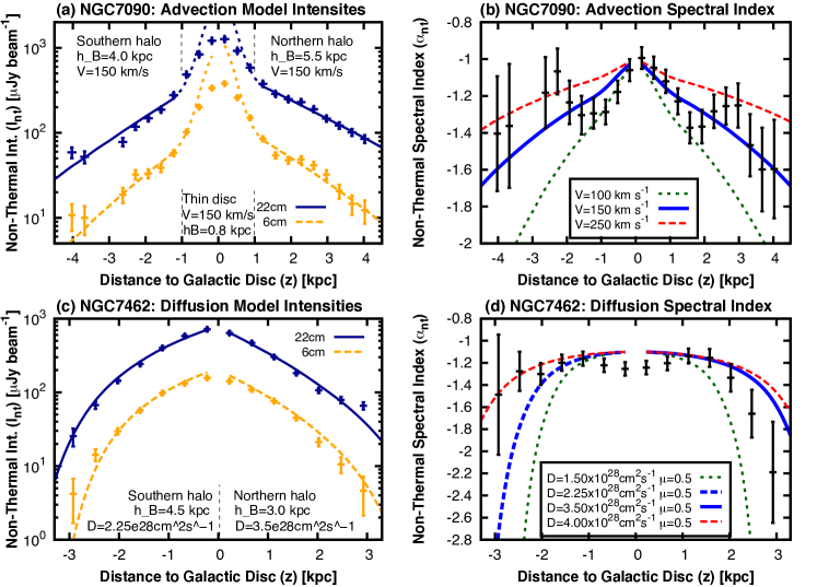
Figure 4: Vertical profiles of the non-thermal radio continuum emission and the non-thermal spectral index in NGC 7090 (averaged between offsets of $\pm 4.25$ kpc, top row) and NGC 7462 (averaged between offsets of $\pm 6.0$ kpc, bottom row). Negative values of $z$ are for the southern halo, and positive ones are for the northern halo. Left panels: modelled profiles from the solution of the 1D cosmic ray transport equations for advection (NGC 7090) and diffusion (NGC 7462) shown as solid, dark-blue ($\lambda$22 cm) and as dashed, orange ($\lambda$6 cm) lines. The short-dashed lines show the thin disc intensities in NGC 7090, not convolved to the resolution, so that they appear not to fit to the data. Right panels: lines show our 1D cosmic ray transport models, with the best-fitting model shown as thick (solid, except in the S halo of NGC 7462) blue line and the error interval indicated by the dashed lines.

3.2 Line-of-sight averaged quantities

The geometry of an edge-on galaxy restricts measurements to averages along the line-of-sight (LoS). The lengths of the lines-of-sight range from several kpc to at least $\approx$10 kpc and, consequently, quantities are averaged over a large variation of galactocentric radii.

3.2.1 Magnetic field strengths

We determine (total) magnetic field strengths $B$ from the revised equipartition formula, using the non-thermal radio continuum intensities at $\lambda 22$ cm as input for the program BFIELD of Beck & Krause (2005). Intensities are converted into surface brightnesses appropriate for a ‘face-on’ view ($i=0\degr$) as function of the offset along the major axis. The non-thermal radio spectral index is another input for BFIELD and is assumed to be $-1.0$. Our measurement between $\lambda\lambda$ 22 and 6 cm resulted into a steeper non-thermal spectral index of $\approx$$-1.25$ (Sect. 3.1.2), but is this probably not representative for the entire spectrum and with most of the energy contained in low-energy cosmic rays, we revert to a more conservative choice. We assume a polarization degree of 10 per cent, where we note that the resulting estimate of the total magnetic field strength depends only weakly on this particular choice (choosing 5 per cent instead makes a difference of less than 1 per cent). Furthermore, we assumed an integration length of 1 kpc perpendicular to the galactic plane, which is appropriate for the radio continuum emission in the thin disc (Sect. 3.1.1) and in accordance with usually used assumptions in the literature (e.g. Niklas & Beck, 1997; Heesen et al., 2014). Lastly, we use $\mathcal{K}=100$ as the number density ratio of the cosmic ray protons to the CRe.

In order to calculate globally averaged magnetic field strengths, we convert the integrated radio continuum flux density into an averaged surface brightness and repeat above analysis. We find that the globally averaged magnetic field strength in NGC 7090 is $8.7~{}\mu\rm G$ and NGC 7462 it is $8.4~{}\mu\rm G$, which is close to $8.4~{}\mu\rm G$, the mean value of the WSRT SINGS sample (Heesen et al., 2014), meaning that our galaxies have very average magnetic field strengths. The average magnetic field strength along the LoS varies between 5 and $13~{}\rm\mu G$, the lower value found in the outskirts of the galaxies and the higher one in the centre. For the area in which we measure scale heights and non-thermal spectral indices, the magnetic field strength is mostly within a range of 8–12 $\mu\rm G$, so that we assume an average magnetic field strength of 10 $\mu\rm G$ in what follows. From the linearly polarized intensity, we can measure the magnetic field strengths of the ordered component in the halo, results of which we will present in Sect. 6.

3.2.2 Photon energy densities

Inverse Compton (IC) radiation losses depend on the energy density of the interstellar radiation field (IRF). It can be described as the superposition of the energy densities of the Cosmic Microwave Background (CMB) with $U_{\rm CMB}=4.2\times 10^{-13}~{}\rm erg\,cm^{-3}$ at redshift zero, the infrared (IR) radiation field, and the stellar (optical) radiation field. Usually the stellar radiation field is scaled to the IR radiation field with $U_{\rm star}=1.73\times U_{\rm IR}$, as derived for the solar neighbourhood (Draine, 2011; Tabatabaei et al., 2013a). The infrared radiation field can be measured from the total IR luminosity. For NGC 7090 we use the prescription by Dale & Helou (2002), using Spitzer 24, 70 and $160~{}\rm\mu m$ luminosities from Dale et al. (2009). For NGC 7462, we use the prescription by Condon (1992), using the IRAS flux densities at 60 and $100~{}\rm\mu m$. A global IR radiation energy density can then be calculated as $U_{\rm IR}=L_{\rm FIR}/(2\pi r_{\rm int}^{2}c)$. Here, $r_{\rm int}$ is the galactocentric radius of the galaxy to which we integrated the radio flux densities, and $c$ is the speed of light. We can calculate the global energy density of the IRF as $U_{\rm rad}=U_{\rm IRF}+U_{\rm CMB}$, where $U_{\rm IRF}=2.73\,U_{\rm IR}$.

In order to obtain a local (kpc scale) IRF energy density, we assume that it scales with $\Sigma_{\rm SFR}$, because the bulk of the dust heating UV-radiation comes from young, massive stars. We find that the average ratio of the photon energy density to that of the magnetic field is $0.31$ (NGC 7090) and $0.18$ (NGC 7462). These values mean that the CRe energy loss rate is dominated by synchrotron over IC radiation losses.

3.2.3 CRe lifetime

In the interstellar medium (ISM), CRe are losing their energy mainly due to synchrotron and IC radiation, so that GeV-electrons have lifetimes of a few $10^{7}~{}\rm yr$. The ionization and bremsstrahlung losses for typical ISM densities of $n=0.05~{}\rm cm^{-3}$ result in lifetimes of the order of $10^{9}~{}\rm yr$ and can hence be neglected (Heesen et al., 2009a), where we assume that cosmic rays are tracing the average density of the ISM within a factor of a few (Boettcher et al., 2013). The combined synchrotron and IC loss rate for CRe is given by (e.g. Longair, 2011):

$$-\left(\frac{{\rm d}E}{{\rm d}t}\right)=b(E)=\frac{4}{3}\sigma_{\rm T}c\left(\frac{E}{m_{\rm e}c^{2}}\right)^{2}(U_{\rm rad}+U_{\rm B}),$$ (4)

where $U_{\rm rad}$ is the radiation energy density, $U_{\rm B}=B^{2}/8\pi$ is the magnetic field energy density, $\sigma_{\rm T}=6.65\times 10^{-25}~{}\rm cm^{2}$ is the Thomson cross section and $m_{\rm e}=511~{}\rm keV\,c^{-2}$ is the electron rest mass. The time dependence of the energy is $E(t)=E_{0}(1+t/t_{\rm rad})^{-1}$, so that at $t=t_{\rm rad}$ the CRe energy has dropped to half of its initial energy $E_{0}$. The CRe lifetime, as determined by synchrotron and IC radiation losses, can be expressed by:

$$t_{\rm rad}=34.2\left(\frac{\nu}{\rm 1~{}GHz}\right)^{-0.5}\left(\frac{B}{\rm 10~{}\mu G}\right)^{-1.5}\left(1+\frac{U_{\rm rad}}{U_{\rm B}}\right)^{-1}~{}{\rm Myr}.$$ (5)

In NGC 7090 and 7462, we find CRe lifetimes, averaged along the lines-of-sight, of 16–60 Myr, with the shorter lifetimes in the centre of the galaxies, where the magnetic field strengths and photon energy densities are highest.

3.2.4 Uncertainties

The equipartition estimate of the magnetic field strength depends on the input values with a power of only $1/(3-\alpha_{\rm nt})=0.25$, so that even large input errors hardly affect the results. If we assume a combined input uncertainty of 50 per cent, arising from the number density ratio, integration length and subtraction of thermal radio continuum emission, our magnetic field uncertainty is $12.5$ per cent. We checked that an uncertainty of $\pm 0.1$ in the non-thermal spectral index has only 3 per cent influence on the magnetic field strength. Consequently, the magnetic field energy density has an uncertainty of $25$ per cent, which is then also the uncertainty of the CRe loss term $b(E)$. In what follows, we do not take this systematic error into account and only derive statistical least-squares fitting errors. But for deriving absolute values of the advection speed and diffusion coefficient, one would have to add it to the error budget.

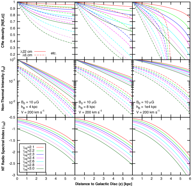
Figure 5: Family of one-zone SPINNAKER advection models with various CRe energy injection indices ($\gamma_{\rm inj}=2.1\ldots 3.0$, note that the order of the lines in the plots and in the legend are identical). The advection speed is $V=200~{}\rm km\,s^{-1}$, the magnetic field strength in the galactic disc is $B_{0}=10~{}\mu\rm G$ and the ratio of the energy densities of the interstellar radiation field to that of the magnetic field is $U_{\rm IRF}/U_{\rm B}=0.3$ (constant ratio everywhere). The magnetic field scale height was varied with $h_{\rm B}=4$ kpc (left panels), $h_{\rm B}=8$ kpc (middle panels) and $h_{\rm B}=10^{4}$ kpc (i.e. constant magnetic field, right panels). Vertical profiles of the CRe number density (top panels) and of the non-thermal radio continuum intensity (middle panels) are for $\lambda$22 cm (solid lines) and for $\lambda$6 cm (dashed line), respectively. The non-thermal radio spectral index between $\lambda\lambda$ 22 and 6 cm is shown in the bottom panels.

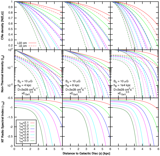
Figure 6: Family of one-zone SPINNAKER diffusion models with various CRe energy injection indices ($\gamma_{\rm inj}=2.1\ldots 3.0$, note that the order of the lines in the plots and in the legend are identical) The diffusion coefficient is $D=3\times 10^{28}E_{\rm GeV}^{0.5}~{}\rm cm^{2}\,s^{-1}$. Otherwise same as Fig. 5.

4 Cosmic ray transport models

4.1 Non-calorimetric numerical models

The vertical profiles of the non-thermal radio continuum emission can be modelled by solving the diffusion–loss equation for the CRe number density $N(E)$ and convolving it with the synchrotron emission spectrum of a single CRe (e.g. Longair, 2011):

$$\frac{{\rm d}N(E)}{{\rm d}t}=D\nabla^{2}N(E)+\frac{\partial}{\partial E}\left[b(E)N(E)\right]+Q(E,t),$$ (6)

where $b(E)=-{\rm d}E/{\rm d}t$ for a single CRe as given by Equation (4). Massive spiral galaxies have rather constant SF histories, so that the CRe injection rate is constant and the source term $Q(E,t)$ has no explicit time dependence. We assume that all sources of CRe a located in the disc plane, neglecting a possible in-situ CRe re-acceleration in the halo, so that for the source term we have $Q(E,t)=0$ for $|z|>0$. Equation (6) can be numerically integrated in time until a stationary solution is found.

We take here a slightly different approach, first by restricting ourselves to a one-dimensional (1D) problem, and second by imposing a fixed inner boundary condition of $N(E,0)=N_{0}E^{-\gamma_{\rm inj}}$. In the stationary case, the change of the CRe number density $\partial N/\partial t$ is solely determined by the energy loss term (second term on the right hand side of Equation (6)). Noticing that for advection we have $\partial N/\partial t=V\partial N/\partial z$, we can re-write Equation (6) for the case of pure advection to:

$$\frac{\partial N(E,z)}{\partial z}=\frac{1}{V}\left\{\frac{\partial}{\partial E}\left[b(E)N(E,z)\right]\right\}\qquad({\rm Advection}),$$ (7)

where $V$ is the advection speed, assumed here to be constant. Similarly, for diffusion we have $\partial N/\partial t=D\partial N^{2}/\partial z^{2}$ (Fick’s second law of diffusion), so that we can re-write Equation (6) for the case of pure diffusion to:

$$\frac{\partial^{2}N(E,z)}{\partial z^{2}}=\frac{1}{D}\left\{\frac{\partial}{\partial E}\left[b(E)N(E,z)\right]\right\}\qquad({\rm Diffusion}),$$ (8)

where we parametrize the diffusion coefficient as function of the CRe energy as $D=D_{0}E_{\rm GeV}^{\mu}$. Usually, values for $\mu$ are thought to be between $0.3$ and $0.6$ (Strong, Moskalenko & Ptuskin, 2007). We assume an exponential magnetic field distribution:

$$B(z)=\left\{\begin{array}[]{ll}B_{0}\cdot\exp(-|z|/h_{\rm B1})\qquad\qquad\qquad\quad(|z|\leq z_{1})\\[5.0pt] B_{0}\cdot\exp(-z_{1}/h_{\rm B1})\cdot\exp(-|z|/h_{\rm B2})\quad(|z|>z_{1}).\end{array}\right.$$ (9)

Here, $h_{\rm B1}$ and $h_{\rm B2}$ are the magnetic field scale heights in the thin and thick disc, respectively, and $z_{1}$ is the transition height between the two.

Equations (7) and (8) can be integrated numerically from the inner boundary. The CRe energy injection spectral index can be obtained from the non-thermal radio spectral index via $\alpha_{\rm nt}=(1-\gamma_{\rm inj})/2$. Further details about the numerical solution of the CRe number density and the calculation of the model synchrotron spectra are provided in Appendix A.

4.2 Fitting procedure

We use the following procedure to fit cosmic ray transport models of either pure diffusion or pure advection to our data: first, we fix the electron energy spectral index in the disc plane, to match the observed non-thermal radio spectral index. Also, we use a representative magnetic field strength in the disc of $B_{0}=10~{}\mu\rm G$ for both galaxies, as averaged in the area, where we have measured non-thermal spectral index profiles (Sect. 3.1.2). IC radiation losses are calculated based on the IRF photon energy density (Sect. 3.2.2). Second, we compute profiles of the CRe number density at $\lambda\lambda$ 22 and 6 cm, to obtain model profiles of both the non-thermal radio spectral index and the non-thermal radio continuum emission. We then fit the radio intensity profiles by varying both the magnetic field scale height and the advection speed (or diffusion coefficient), resulting in the reduced $\chi^{2}$:

$$\chi^{2}=\frac{1}{N-n}\sum\left(\frac{I_{i}-M_{i}}{\sigma_{i}}\right).$$ (10)

Here, $I_{i}$ is the $i$th non-thermal intensity measurement, $M_{i}$ the corresponding model value, $\sigma_{i}$ the error of the measured intensity, $N$ the number of data points and $n$ the number of fitted parameters. We use $n=3$, because we fit also for the intensity normalization. The reduced $\chi^{2}$ is shown in Fig. 7 with our best-fitting models presented in Fig. 4 (see Table 5 for the best-fitting parameters).

4.3 Calorimetric analytical models

We can compare our results with the ‘calorimetric’ advection and diffusion models employed by Heesen et al. (2009a), who assumed:

$$h_{\rm e}=\left\{\begin{array}[]{ll}V\cdot t_{\rm rad}\qquad({\rm Advection}),\\[5.0pt] \sqrt{D\cdot t_{\rm rad}}\quad({\rm Diffusion}).\end{array}\right.$$ (11)

This are meaningful only if the electron radiation losses are dominating the vertical decrease in the non-thermal radio continuum intensity, an assumption that appeared to be justified in the starburst galaxy NGC 253, where above relations provided good fits to the data (Heesen et al., 2009a). This is the case the magnetic field strength is constant in the halo and the galaxy constitutes and electron calorimeter, hence we refer to these models as the calorimetric ones. It is also noted that Heesen et al. (2009a) calculated $h_{\rm e}$ assuming energy equipartition, which may not hold in the halo, where the CRe either escape almost freely or are losing the bulk of their energy via synchrotron and IC radiation. Furthermore, the relation for diffusion neglects any possible energy dependence of the diffusion coefficient. It is one of the scopes of this work, to test whether the calorimetric models can be applied to normal star forming galaxies, where the outflow speeds may be sufficiently high, so that CRe radiation losses do not dominate in the halo.

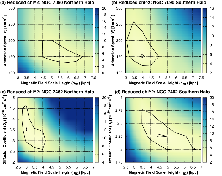
Figure 7: Reduced $\chi^{2}$ for the advection model in NGC 7090 (top panels) and the diffusion model in NGC 7462 (bottom panels). Contours indicate the best-fitting reduced $\chi_{\rm min}^{2}$ (inner contours) and $\chi_{\rm min}^{2}+1$ (outer contours). Values in NGC 7462 were clipped at $\chi^{2}=20$.

5 Cosmic ray transport

In this section, we apply our 1D cosmic ray transport models created with SPINNAKER to the radio continuum observations of NGC 7090 and 7462 (Sects 5.2 and 5.3). This is preceded by Sect. 5.1, where we present some general results of our modelling that can help to decide whether diffusion or advection is dominating. In Sect. 5.4 we investigate the scale height–CRe lifetime relation, an analysis equivalent to that of Heesen et al. (2009a).

5.1 The distinction between advection and diffusion

In Figs 5 and 6 we present families of one-zone advection and diffusion models created with our numerical cosmic ray transport models (Sect. 4). We use a typical magnetic field strength of $B_{0}=10~{}\mu\rm G$ and a ratio of the interstellar radiation field energy density to magnetic field energy density of $U_{\rm IRF}/U_{\rm B}=0.3$, assumed to be constant everywhere. We varied the magnetic field scale height, with one set of models using $h_{\rm B}=4$ kpc, the second one $h_{\rm B}=8$ kpc and the third one $h_{\rm B}=10^{4}$ kpc (constant magnetic field). We varied the CRe injection spectral index between $\gamma_{\rm inj}=2.1\ldots 3.0$. The CRe number density was calculated for $\lambda\lambda$ 22 and 6 cm as well as the resulting non-thermal radio continuum intensities and corresponding non-thermal radio spectral indices. For the advection models we used a constant advection speed of $V=200~{}\rm km\,s^{-1}$, whereas for the diffusion models we used $D=3\times 10^{28}E_{\rm GeV}^{0.5}~{}\rm cm^{2}\,s^{-1}$.

Table 5: Model parameters in the northern (N) and southern (S) haloes.

Parameter	NGC 7090 (N/S)	NGC 7462 (N/S)
$B_{0}$ (fixed) [$\mu$G]	10	10
$z_{1}$ (fixed) [kpc]	1	$-$
$h_{\rm B1}$ (fixed) [kpc]	$0.8$	$-$
$\gamma_{\rm inj}$ (fixed)	$3.0$	$3.2$
$U_{\rm IRF}/U_{\rm B}$ (fixed)	0.31	0.18
$V$ (var.) [$\rm km\,s^{-1}$]	$150^{+50}_{-20}/150^{+100}_{-30}$	$-$
$D_{0}$ (var.) [$\rm cm^{2}\,s^{-1}$]	$-$	$(3.5^{+1.2}_{-0.8}/2.25^{+0.5}_{-0.2})10^{28}E_{\rm GeV}^{0.5}$
$h_{\rm B2}$ (varied) [kpc]	$5.5^{+1.3}_{-1.0}/4.0^{+1.0}_{-0.9}$	$3.0^{+1.2}_{-0.25}/4.5^{+2.2}_{-1.0}$
$\chi^{2}$ (minimum)	$1.5$/$2.6$	$4.3$/$2.4$

Cosmic ray electron number density. It is instructive to first analyse how the vertical profile the CRe number density evolves for either a pure advection or diffusion model. If the advection speed is sufficiently high (or the magnetic field scale height sufficiently small), the CRe number density decreases monotonically, but with a decreasing slope, so that it almost approaches an asymptotic value (Fig. 5, top panels). In contrast, diffusion will always lead to a sharp cut-off in the CRe number density (Fig. 6, top panels).

Non-thermal radio continuum emission profiles. We found that advection results in approximately exponential profiles (Fig. 5, middle panels), whereas diffusion results in profiles, which are reminiscent of Gaussian functions (Fig. 6, middle panels). The exact shape of the profile depends obviously on the combination of the magnetic field scale height and either diffusion coefficient or advection speed. If CRe radiation losses are unimportant, we expect exponential profiles caused by the decrease of the magnetic field strength only. If CRe radiation losses are important, both diffusion and advection will have cut-offs in their profiles, where the intensity decreases rapidly. If radiation losses are important, but the decrease of the magnetic field plays a role as well, we expect to see a mix of the profiles of the CRe number density and the magnetic field. In general it can be said, that advection will result in profiles that are to a good approximation exponential, although at large $z$ it is steeper than an exponential profile. Diffusion leads to profiles that are exponential at small $z$, where the decrease of the magnetic field dominates. At large $z$, a strong steepening is observed due to large CRe radiation losses. Hence, a diffusion profile is steeper both at small and large $z$ than a Gaussian profile would predict.

Non-thermal radio spectral index profiles. For advection, the non-thermal radio spectral index steepens rather gradually with increasing distance from the disc (Fig. 5, bottom panels). The profile can be approximated by a linear function, with the curvature only becoming more prominent if the magnetic field is constant. For diffusion, the profile of the non-thermal radio spectral index has a characteristic shape, where the slope is very flat in the inner part and progressively steepens dramatically in the outer parts (Fig. 6, bottom panels). We have chosen $\mu=0.5$; a higher energy dependence of the diffusion coefficient ($0.5<\mu\leq 0.7$), leads to less steepening, contrary, a lower energy dependence ($0\leq\mu<0.5$) steepens the spectral index.

Non-thermal radio continuum scale heights. One important result of our modelling is that it is always possible to find a good fit to the profile of the non-thermal spectral index, choosing an appropriate combination of advection speed (or diffusion coefficient) and magnetic field scale height. A large magnetic field scale height can be balanced by either a large advection speed or diffusion coefficient. But this has an effect on the non-thermal radio continuum scale heights, leading to higher values as well. The combination of spectral index profiles and radio continuum scale heights constrains both parameters fairly well.

5.2 Cosmic ray transport in NGC 7090

5.2.1 Advection or diffusion?

NGC 7090 has a thin and a thick radio disc (Sect. 3.1.1), so that we modelled the magnetic field accordingly with a two-component exponential profile (with the thin disc at $|z|\leq 1$ kpc). As pointed out in Sect. 3.1.1, we can not distinguish between an approximately exponential or Gaussian profile, so that we modelled the thin/thick disc with an advection/advection, advection/diffusion, diffusion/advection and diffusion/diffusion model in order to cover all possible combinations. The vertical profiles of the radio spectral index shown in Fig. 4(b) display a characteristic steepening in the inner parts at $|z|\leq 2$ kpc and a possible flattening at larger heights, which has to be explained by the modelling. We can rule out a diffusion/diffusion model ($\chi^{2}=8$, both haloes), where the steep spectral index in the thin disc at $|z|\leq 1$ kpc requires a small diffusion coefficient of $D\approx 0.5\times 10^{28}E_{\rm GeV}^{0.5}~{}\rm cm^{2}\,s^{-1}$, which results in no significant emission in the thick disc regardless of the diffusion coefficient chosen there. This can be understood in such a way that the diffusion coefficient prescribes the curvature rather than the slope of $N(E,z)$. Hence, even increasing the diffusion coefficient in the thick disc to large values (a few $10^{29}E_{\rm GeV}^{0.5}~{}\rm cm^{2}\,s^{-1}$), will still result in too low emission levels. Notably an advection/diffusion model works, but it is unphysical, because we would expect a galactic wind or outflow to become more efficient further away from the disc.

Hence, advection has to dominate in the thick disc, which leaves the advection/advection and diffusion/advection models that describe the data equally well ($\chi^{2}=1.3$–$2.3$). The thin disc can be fitted by $h_{\rm B1}=0.8\pm 0.1$ kpc with either $D=0.5^{+0.2}_{-0.1}\times 10^{28}E_{\rm GeV}^{0.5}~{}\rm cm^{2}\,s^{-1}$ or $V=150\pm 50~{}\rm km\,s^{-1}$. In the thick disc, the minimum advection speed is $100~{}\rm km\,s^{-1}$ with the upper limit unconstrained, since the radio spectral index does not steepen in the halo (Fig. 4(b)). This shows that the advection speed is sufficiently high, so that radiation losses are not dominating in the halo.

5.2.2 Best-fitting advection model

In order to better constrain the value of the advection speed, we fitted an advection/advection model with equal advection speeds in the thin and thick disc. The upper limit of the advection speed is then largely determined by the thin disc and may be potentially higher in the thick disc. In Fig. 7(a) we show the reduced $\chi^{2}$ as function of advection speed and magnetic field scale height in the thick disc. The best-fitting parameters are an advection speed of $V=150^{+50}_{-20}~{}\rm km\,s^{-1}$ and a magnetic field scale height of $h_{\rm B2}=5.5^{+1.3}_{-1.0}$ kpc in the northern halo and $V=150^{+100}_{-30}~{}\rm km\,s^{-1}$ and $h_{\rm B2}=4.0^{+1.0}_{-0.9}$ kpc in the southern halo. The parameters used in the fitting procedure are summarized in Table 5. It is instructive to compare the magnetic field scale heights with the values that we would obtain from equipartition. In the northern halo we would expect a magnetic field scale height of $6.8$ kpc (assuming a non-thermal spectral index of $\alpha_{\rm nt}=-1$) and in the southern halo of $6.1$ kpc (from the $\lambda$22 cm scale heights). Hence, the scale heights as inferred from our modelling are 20–35 per cent lower than the equipartition values. This is suggests that the assumption of energy equipartition breaks down in the halo.

A complication we have not yet discussed is the fact that the thin disc consists of a mix of young and old CRe, so that the radio spectral index may not be representative for the CRe that actually enter the outflow. It is conceivable that the spectral index steepening within the first 2 kpc distance from the galactic disc is largely due to the decreasing influence of the thin disc, containing some young, freshly injected CRe. Such a scenario is consistent with a diffusion dominated transport in the thin disc, where the CRe population at any given position is a mix of young and old electrons. As pointed out above, if we fit a diffusion/advection model, the advection speed can be potentially significantly higher in the halo. An advection of $V=250~{}\rm km\,s^{-1}$, at the upper end of the error interval, would fit well (compare Fig. 4(a)). The same effect can be created by underestimating the thermal radio continuum emission due to internal absorption of Balmer H$\alpha$ line emission by dust (Sect. 2.2). Hence, our advection speeds are conservative lower limits.

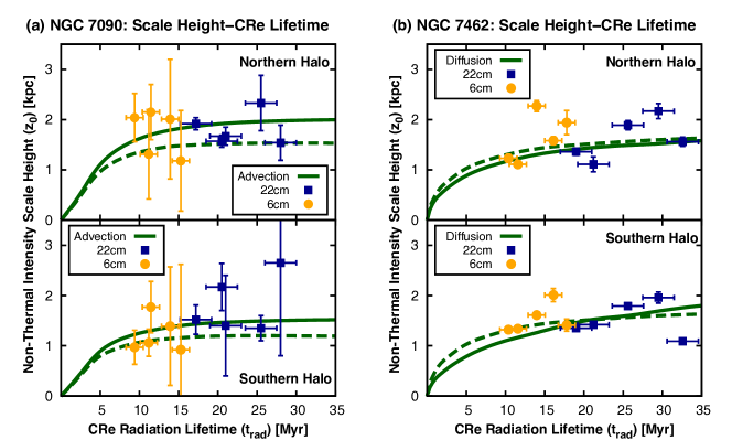
Figure 8: Non-thermal radio continuum scale heights as function of the CRe lifetime at $\lambda\lambda$ 22 cm (dark-blue) and 6 cm (orange). Left: NGC 7090, where scale heights of the thick exponential disc are plotted. Right: NGC 7462, where scale heights of the Gaussian disc are plotted. The green, solid (dashed) dark-green line shows the predicted scale heights from the best-fitting transport model at $\lambda$22 cm ($\lambda 6~{}\rm cm)$.

5.3 Diffusive cosmic ray transport in NGC 7462

In NGC 7462, we did not find a thin disc (Sect. 3.1.1), so that we modelled the magnetic field with a one-component exponential function describing the thick disc only. The Gaussian vertical radio continuum profiles suggest diffusion as the dominating transport mode (Fig. 4(c)). The vertical spectral index profile corroborates shown in Fig. 4(d) this scenario, with a flat spectral index within $|z|\leq 2$ kpc and a significant steepening for heights $|z|>2$ kpc; the spectral index profile has a parabolic shape. In the southern halo, diffusion ($\chi^{2}=2.4$) describes the data significantly better than advection ($\chi^{2}=12$). In the northern halo, diffusion ($\chi^{2}=4.3$) describes the data marginally worse than advection ($\chi^{2}=3.9$); this is largely due to the extended emission that can be seen at $\lambda$22 cm at $z>2$ kpc (Fig. 3(b) at offsets $-2.4$ and 0 kpc). We believe that diffusion is the more likely transport mode, because a ‘one-sided’ galactic wind appears to be an unlikely scenario. Also, advection does not reproduce the parabolic spectral index shape, but leads to a linear steepening of the spectral index, in contrast to what is seen in the observations. For completeness, we present here the best-fitting advection parameters in the northern halo as $V=200^{+200}_{-30}~{}\rm km\,s^{-1}$ and $h_{\rm B2}=3.0^{+0.25}_{-1.2}$ kpc.

In Fig. 7(b), the reduced $\chi^{2}$ of the spectral index fitting as function of the diffusion coefficient and magnetic field scale height is presented. Our best-fitting parameters are a diffusion coefficient of $3.5^{+1.2}_{-0.8}$ and $2.25^{+0.5}_{-0.2}\times 10^{28}E_{\rm GeV}^{0.5}~{}{\rm cm^{2}\,s^{-1}}$ and a magnetic field scale height of $3.0^{+1.2}_{-0.25}$ and $4.5^{+2.2}_{-1.0}$ kpc in the northern and southern halo, respectively. We note that the average CRe energy within our wavelength range is $4.2$ GeV, so that the actual diffusion coefficient is a factor of $\approx$2 higher than $D_{0}$. We have varied the energy dependence of the diffusion coefficient $\mu$ and found that for $\mu=0.3\ldots 0.7$, the diffusion coefficient (normalized to $E=4.2$ GeV) changes by less than 10 per cent and the magnetic field scale height changes by less than 17 per cent. The parameters used in the fitting procedure are summarized in Table 5. The diffusion coefficients we find are in good agreement what is reported in the literature for diffusion within the disc plane (e.g. Murphy et al., 2008; Fletcher et al., 2011; Heesen et al., 2011; Buffie et al., 2013; Berkhuijsen et al., 2013; Tabatabaei et al., 2013b; Mulcahy et al., 2014). This means that NGC 7462 is an example for a galaxy, where cosmic rays are just diffusing from the disc into the halo and advection plays no role.

Finally, as noted earlier (Sect. 3.1.1), it may be possible that the radio continuum profiles are exponential, if the baselevel of our map is negative by $\approx$$-1\sigma_{\rm TP}$. However, the profiles of the non-thermal radio spectral index are still in agreement with diffusion only. Our model has to explain why the spectral index remains constant within $|z|\leq 1.1$ kpc, where $S/N>10$, so that the baselevel uncertainty does not play a role. Advection only leads to parabolic spectral index profiles, if the magnetic field scale height is large ($\gtrsim$10 kpc). In this case, the resulting radio continuum scale height is, however, much larger than the measured $0.9$ kpc for an exponential profile. The only way out is that our non-thermal radio spectral index profiles are biased to too steep spectral indices within $|z|<2$ kpc, for instance by subtracting a too high thermal fraction of radio continuum emission due to our uncertain calibration procedure (Sect. 2.2); this is corroborated by the local minimum of the non-thermal spectral index in the disc plane. On the other hand, we expect the Balmer H$\alpha$ emission to underestimate the thermal radio continuum, because we did not take absorption due to dust into account. Thus, we conclude that the measurement of a steep spectral index in the disc plane is robust and, consequently, cosmic ray diffusion is the dominating transport mode in NGC 7462.

5.4 Scale height–lifetime relation

Our cosmic ray transport models (Sect. 4) are fitted to the data averaged over a wide range of galactocentric radii, so that we are not sensitive to variations of the advection speed or diffusion coefficient as function of position. Ideally, we would like to apply our models locally (kpc scale), but the low S/N of the halo emission prevents us from doing so. What we can do instead, is to analyse the dependence of the local scale heights derived in the stripes of Sect. 3.1.1) ($\approx$2 kpc width), as function of the CRe lifetime; so we can check whether they are consistent with our cosmic ray transport models.

The scale heights of both galaxies, presented in Fig. 8, do not show any clear dependence of the CRe lifetime. The average Pearson’s rank order correlation coefficient is with $r_{\rm s}=0.23$ so low ($r_{\rm s}=0\ldots 1$, for a positive correlation), that we conclude that no linear trend is observed. Our models (shown as green lines) reproduce this (non-existing trend) well: for CRe lifetimes in excess of 15 Myr the scale heights are almost constant, since the decrease of the magnetic field dominates the decrease of the non-thermal intensity (non-calorimetric halo). Only for lifetimes smaller than 10 Myr we would expect a decrease of the scale heights, but since we are not probing this regime we can not verify this particular prediction. The model reproduces the scale heights of NGC 7090 well within the uncertainties, although it fails to explain the variation of the local scale heights in NGC 7462. In the latter case, the error bars are small because the single Gaussian fits are well constrained by data points within $|z|<3$ kpc, which have a high S/N (Sect. 3.1.1).

As a further consistency check, we fit our calorimetric transport models from Equation (11), where we utilise the usual assumption of energy equipartition for which the CRe scale height is:

$$h_{\rm e}=\frac{3-\alpha_{\rm nt}}{2}z_{0},$$ (12)

where we assume $\alpha_{\rm nt}\approx-1$ and where $z_{0}$ is the non-thermal radio scale height of the thick disc (Sect. 3.1.1). In NGC 7090, we find advection speeds of $186$ and $144~{}\rm km\,s^{-1}$ in the northern and southern halo, respectively. This is in good agreement with our models. However, we point out that the magnetic field strength in the halo ($|z|>1$ kpc) is lower, $B\leq 3~{}\rm\mu$G, than what we used for our calorimetric approximation ($B=10~{}\mu$G, $B$=const.). Therefore, the actual CRe lifetime is a factor of five longer (Equation (5)), so that CRe scale height must be a factor of five higher as well. The agreement between calorimetric and non-calorimetric model is in the case of NGC 7090 thus coincidental. Similarly, in NGC 7462 we find a calorimetric diffusion coefficient of $1.4\times 10^{29}~{}\rm cm^{2}\,s^{-1}$ both in the northern and southern halo of NGC 7462 (no energy dependence, $\mu=0$). This is a factor of two higher than the value derived by our models. The reason is again that we have overestimated $B$; at 2 kpc height, the average height where we determined the scale height, the magnetic field strength is only 60 per cent of the one in the disc, so that the CRe lifetime increases by a factor of two.

In summary, we find that the scale heights measured in stripes are broadly consistent with a constant diffusion coefficient and advection speed across the width of the galactic disc, as assumed for our modelling. But the numerical values obtained from the calorimetric approximation can be used only if (i) the CRe scale heights estimated from equipartition are accurate and (ii) the average halo magnetic field strength can be estimated.

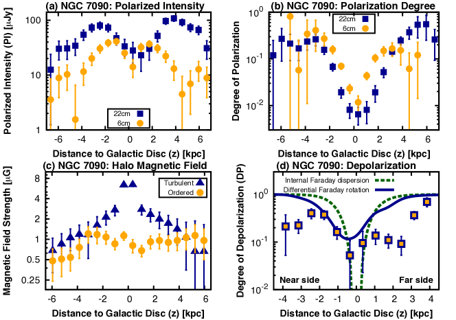
Figure 9: Vertical profiles used for the analysis of the linearly polarized intensity in NGC 7090, averaged between offsets of $\pm 4.25$ kpc (panels a,b,c) and $\pm 0.75$ kpc (d) along the major axis. Negative values of $z$ are for the southern halo, and positive ones are for the northern halo. Top left: polarized intensity at $\lambda\lambda$ 22 (dark-blue) and 6 cm (orange). Top right: Degree of polarization at $\lambda\lambda$ 22 (dark-blue) and 6 cm (orange). Bottom left: magnetic field strength of the turbulent and ordered magnetic field in the halo. Bottom right: Degree of depolarization between $\lambda\lambda$ 22 and 6 cm. The dark-green line shows a model profile of internal Faraday dispersion by turbulence in the magneto-ionized ISM and the dark-blue line shows a model for Faraday dispersion by the regular halo magnetic field (see text for details).

6 Halo magnetic field

6.1 Morphology

In Figs 1 and 2 (panels (c) and (d)) we present the distribution of the linearly polarized intensity in NGC 7090 and 7462 at $\lambda\lambda$ 22 and 6 cm, respectively. In a magnetized plasma a polarized wave vector is rotated by Faraday rotation. For a uniform magnetic field and (thermal) electron density, we define the rotation measure (RM) via:

$$\frac{\Delta\phi}{\rm rad} = 0.808\times\left(\frac{\lambda}{\rm m}\right)^{2}{\int}_{0}^{\frac{L}{\rm pc}}\left(\frac{B_{\rm reg\parallel}}{\mu\rm G}\right)\left(\frac{n_{\rm e}}{\rm cm^{-3}}\right){\rm d}\left(\frac{l}{\rm pc}\right)$$

$$= 0.808\lambda^{2}{\rm RM},$$

where $n_{\rm e}$ is the thermal electron density, $B_{\rm reg\parallel}$ is the LoS component of the regular magnetic field and $L$ is the integration length through the magneto-ionized medium. The maximum RM value we measure between $\lambda\lambda$ 22 and 6 cm is $\pm 40~{}\rm rad\,m^{-2}$ (Figs 1(d) and 2(d)), which is not enough to correct for Faraday rotation in an edge-on galaxy; the galaxies are partially depolarized at $\lambda$22 cm, so that one can not measure the RM reliably. Thus, the magnetic field orientations presented in this work are not corrected for Faraday rotation. A maximum RM amplitude of $40~{}\rm rad\,m^{-2}$ requires differential Faraday rotation (Sokoloff et al., 1998), either by an ordered disc or halo magnetic field, with a coherent direction over kpc-scales, also referred to as ‘regular’ magnetic field.

We find that NGC 7090 features a prominent polarized radio halo, particularly at $\lambda$22 cm (Fig. 1(c)), where we can detect polarized emission up to heights of 6 kpc in the northern halo and 4 kpc in the southern halo. The polarized emission at $\lambda$22 cm is asymmetric with respect to the minor axis, where the bulk of polarized emission is located on the approaching side of the galaxy (see Dahlem et al., 2005, for an H I rotation curve of the galaxy). This is in agreement with findings of Braun, Heald & Beck (2010), who postulated that this kind of asymmetry can be explained by depolarization due to differential Faraday rotation caused by a magnetic field structure, which consists of a disc magnetic field and a quadrupolar halo magnetic field. But their model is not applicable in our case, since it works only for galaxies at moderate inclination angles from 20–$70\degr$. For an alternative explanation we note that the western side of the galaxy has a higher star formation rate, as indicated by the higher radio continuum intensity (Figs 1(a) and (b)). The asymmetry of polarized emission with respect to the minor axis may thus be a consequence of the asymmetric S/N. In Figs 1(c) and (d) we can see evidence of depolarization by the combined effects of the turbulent magnetic field in the disc and by differential Faraday rotation due to the ordered (more precisely regular) magnetic field in the disc and halo, both at $\lambda\lambda$ 22 and 6 cm; but no direct evidence of an ordered disc magnetic field itself is seen, probably due to depolarization as well, in part also caused by depolarization due to unresolved vertical $E$-vectors within the beam area.

In NGC 7462, the bulk of the polarized emission at $\lambda$22 cm (Fig. 2(c)) is again found on the approaching side of the galaxy, concentrated in a filamentary region of 10 kpc length and $2.6$ kpc width. It is probably related to the very extended extra-planar component only detected at $\lambda$22 cm (Sect. 3.1.1); this would explain why almost none of the polarized emission is seen at $\lambda$6 cm (Fig. 2(d)). The integrated H I map of Dahlem et al. (2005) shows that the H I distribution in the eastern half of the galaxy is thicker than in the western half. Hence, we may speculate that we are seeing the remnants of an outflow, which stirred up the H I disc and where the CRe are still visible as aged radio continuum emission with a steep spectral index. Another prominent feature is a ‘spur’ of polarized emission centred on RA $23^{\rm h}02^{\rm m}47^{\rm s}$ Dec. $-40\degr 50\arcmin 00\arcsec$. It may be connected to the extended emission which we masked (Sect. 3), although it does not align exactly with it and is more reminiscent of a jet-driven lobe, emerging from the galaxy’s centre. As mentioned earlier, we did not find any unresolved source in the centre of the galaxy, hinting at past or current AGN activity. In any case, the emission is probably not related to any galactic outflow, which NGC 7462 probably does currently not possess anyway, being diffusion dominated. Hence, we continue our analysis with NGC 7090 only.

6.2 Magnetic field strengths and depolarization

We can now measure the strength of the ordered halo magnetic field. To this end, we investigate vertical profiles of the linearly polarized emission and degree of polarization as presented in Fig. 9(a) and (b) (see Appendix B for the tabulated values). The degree of polarization $p$ relates to the ratio $q=B_{\rm turb}/B_{\rm ord,\perp}$ of the isotropic turbulent magnetic field $B_{\rm turb}$ to the ordered magnetic field in the plane of the sky $B_{\rm ord,\perp}$ via:

$$\frac{p}{p_{0}}=\frac{1}{1+q^{2}},\qquad p_{0}=\frac{3-3\alpha_{\rm nt}}{5-3\alpha_{\rm nt}},$$ (14)

where $p_{0}$ is the theoretically maximum polarization degree for a purely uniform magnetic field. In above relation we used that the polarized (total) synchrotron intensity scales with $PI\propto B_{\rm ord,\perp}^{2}$ ($I_{\rm nt}\propto B^{2}$) for $\alpha_{\rm nt}=-1$, so that $p/p_{0}=B_{\rm ord,\perp}^{2}/B^{2}$. We now use the assumption that the ordered magnetic field is in the plane of the sky, $B_{\rm ord}=B_{\rm ord,\perp}$, so that we can calculate the ordered field strength as $B_{\rm ord}=B(1+q^{2})^{-1/2}$ and the turbulent magnetic field strength as $B_{\rm turb}=(B^{2}-B_{\rm ord}^{2})^{1/2}$. We use the $\lambda$22 cm degree of polarization at $|z|>3.5$ kpc and the $\lambda$6 cm degree of polarization elsewhere. This is because the $\lambda$22 cm observations are more severely affected by depolarization, but extend away further from the galactic midplane. The vertical profiles of the turbulent and ordered magnetic field strength are shown in Fig. 9(c). The ordered magnetic field strength ranges largely between $0.5$ and $1~{}\rm\mu G$, whereas the turbulent magnetic field strength decreases monotonically from $10~{}\mu\rm G$ at $z=0$ to $1~{}\mu\rm G$ at $z=5$ kpc.

For further analysis, we introduce the degree of depolarization (DP), defined as the ratio of the polarization degrees at two wavelengths, which is usually calculated using the ratio of the (linearly) polarized intensities and the non-thermal radio spectral index:

$${\rm DP}\equiv\frac{PI_{22}}{PI_{6}}\times\left(\frac{\nu_{6}}{\nu_{22}}\right)^{\alpha_{\rm nt}},$$ (15)

where $PI_{22}$ and $PI_{6}$ are the polarized intensities at $\lambda\lambda$ 22 and 6 cm, respectively, and $\nu_{22}=1.4$ and $\nu_{6}=4.7$ GHz are the corresponding frequencies. We found a pronounced minimum of the degree of depolarization surrounding the galactic midplane of NGC 7090, as shown in Fig. 9(d). There is a steep rise in the degree of depolarization in the southern halo ($-3\leq z\leq 0~{}\rm kpc$). For illustration, we compare it with a depolarization model for Faraday dispersion by turbulence in the magneto-ionized ISM (Burn, 1966; Sokoloff et al., 1998):

$$\mathcal{P}_{\rm disp}=p_{\rm i}\frac{1-\exp(-2\sigma_{\rm RM}^{2}\lambda^{4}Ld^{-1})}{2\sigma_{\rm RM}^{2}\lambda^{4}Ld^{-1}}.$$ (16)

Here, $\sigma_{\rm RM}(z)=0.808\times n_{\rm e}(z)\times d\times B_{\rm turb,\parallel}(z)$, where $d$ is the size of the turbulent eddies in pc, $B_{\rm turb,\parallel}$, the LoS component of the turbulent magnetic field in $\mu\rm G$, $L$ the length of the LoS in pc and $n_{\rm e}$ the thermal electron density in $\rm cm^{-3}$. The intrinsic degree of polarization $p_{\rm i}$ can be eliminated by using two wavelengths and forming the ratio to measure the degree of depolarization. We have assumed an electron density of $0.02~{}\rm cm^{-3}$ and a scale height of $1.5$ kpc, in loose agreement with values for the Milky Way (Ferrière, 2001). We used 100 pc as the size of the turbulent eddy in the disc plane (see Fletcher et al., 2011, for a measurement in an external galaxy). We find that Faraday dispersion explains our data partially, although the model over-predicts the depolarization in the disc and under-predicts it in the halo. One would have to increase the electron scale height to values of 4 kpc in order to get agreement with the data in the southern halo. Another source of depolarization is differential Faraday rotation due to a regular disc magnetic field with a coherent direction, for which the model is:

$$\mathcal{P}_{\rm diff}=p_{i}\frac{\sin(\mathcal{R}\lambda^{2})}{\mathcal{R}\lambda^{2}},$$ (17)

where $\mathcal{R}=0.808\times n_{\rm e}(z)\times d\times B_{\rm reg,\parallel}(z)$ and $B_{\rm reg,\parallel}(z)$ is the regular magnetic field component along the LoS (which we assumed to be equal to the ordered field strength). We find that this model can explain the depolarization in the southern halo ($-2\leq z\leq-1$ kpc) better. Where our depolarization models all fail is north of the galactic midplane ($0\leq z\leq 2$ kpc), where the degree of depolarization is low and rises steeply further away from the disc. A possible explanation is that the turbulent magnetic field in the disc depolarizes the northern halo, which hence is on the far side, whereas the southern halo has to be on the near side (we have overlaid in Fig. 1(c) the optical extent of the disc for comparison). However, it is difficult to come to any firm conclusion without a more comprehensive modelling of the magnetic field structure, such as the three-dimensional magnetic field models employed by Heesen et al. (2009b, 2011).

The magnetic field in NGC 7090 appears to be dominated by the halo component (Fig. 1(d)), although shorter wavelengths would be required to exclude depolarization of a disc magnetic field. This suggests a relation to a galactic wind or outflow. A galactic wind facilitates an efficient halo dynamo (Moss et al., 2010); an outflow stretches magnetic field lines into Parker-type loops (Mao et al., 2015). The former process results in regular magnetic fields, the latter in anisotropic ones. Observations at shorter wavelengths are needed to measure Faraday rotation and distinguish between the two scenarios.

7 Discussion

The outflow of cosmic rays has important ramifications for the observed relation between the star formation rate (SFR) and the radio continuum (RC) luminosity, in the following RC–SFR relation (Condon, 1992; Heesen et al., 2014). The widely used semi-empirical ‘Condon relation’ assumes that galaxies are electron calorimeters. This would imply that the CRe lose all their energy exclusively within the galaxy, or, more precisely, we are observing always the same fraction of possible non-thermal synchrotron emission. This was already postulated by Völk (1989), who predicted that the radio continuum emission of a galaxy should, in case of a CRe calorimeter, only be a function of the ratio of IC to synchrotron losses. But observational tests are at odds with the calorimetric theory. The non-thermal radio spectral index would have to be quite steep, $\approx$$-1.2$ (Lisenfeld & Völk, 2000), which does not agree with the observed spectral index, where studies find spectral indices of $-0.83$ (Niklas, Klein & Wielebinski, 1997), $-0.8$ (Marvil, Owen & Eilek, 2015). Furthermore, Heesen et al. (2014) found that in spiral galaxies the average ratio of IC to synchrotron losses is only 30 per cent, which means that we cannot easily test the prediction by Völk (1989). The alternative are non-calorimetric models, which assume (i) energy equipartition between the cosmic rays and the magnetic field, and (ii), a relation between either the magnetic field strength and gas density (Niklas & Beck, 1997), or a relation between the magnetic field strength and star formation rate (Heesen et al., 2014).

Non-electron calorimetry can be caused, if the advection speed is sufficiently high, so that the CRe lifetime is longer than the CRe escape time: $t_{\rm rad}\gg t_{\rm esc}$. The escape time is here defined as the $t_{\rm esc}=h_{\rm B}/(2V)$, where $h_{\rm B}/2$ is the scale height of the magnetic field energy density, assuming that the non-thermal intensity scales with the magnetic field as $I_{\rm nt}\propto B^{2}$ (exact for $\alpha_{\rm nt}=-1$). We now define the equivalent advection speed, where the CRe lifetime (Equation (5)) is equal to the CRe escape time:

$$V_{\rm equiv}\equiv\frac{h_{\rm B}}{2\,t_{\rm rad}}=200~{}{\rm km\,s^{-1}}~{}\left(\frac{h_{\rm B}}{\rm 4~{}kpc}\right)\left(\frac{t_{\rm rad}}{\rm 10~{}Myr}\right)^{-1}.$$ (18)

For example, in the northern halo of NGC 7090 ($B=3.3~{}\mu\rm G$ at $z=1~{}\rm kpc$, the base of the halo), the CRe lifetimes are $110$ and $60$ Myr at $\lambda\lambda$ 22 and 6 cm, so that the equivalent advection speeds are 25 and 50 km s^-1, respectively. At higher wind speeds, the CRe are transported faster along the gradient of the magnetic field and stellar photon energy density than they lose their energy via synchrotron and IC radiation. They are able to retain a non-vanishing fraction of their initial energy and the galaxy is not an electron calorimeter.

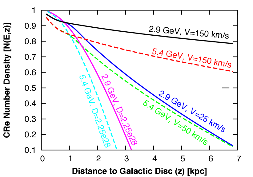
Figure 10: Profiles of the CRe number density at $\lambda\lambda$ 22 and 6 cm (solid and dashed lines), equivalent to CRe energies of $2.9$ and $5.4$ GeV, respectively, for the northern halo of NGC 7090 (advection) and for the southern halo of NGC 7462 (diffusion).

Profiles of the CRe electron energy distributions for the northern NGC 7090 are shown in Fig. 10. For our best-fitting model, at the detection limit of the halo, $z=7$ kpc, the CRe number density has dropped by less than 40 per cent, so that the CRe retain at least 60 per cent of their energy at 7 kpc height. In contrast, if the advection speed is dropped to the critical speed (at $z>1$ kpc), the CRe number density drops by 90 per cent. At $\lambda$22 cm, equivalent to a CRe energy of $2.9$ GeV, the CRe number density is at least 70 per cent at 7 kpc, the limit to which we can observe the halo. This means that we potentially lose up to 70 per cent of the potential radio luminosity, but we should keep in mind that the CRe number density refers to those electrons that are able to leave the thin radio disc. The thin radio disc has a non-thermal radio spectral index of $-1.0$, so that the electron have already lost some of their energy, before they are able to enter the outflow. In the thin radio disc, one probably has a mix of young, freshly injected CRe, and older ones, which are enclosed in the SNe heated superbubbles, before they are able to break out from the disc (Heesen et al., 2015). In contrast, diffusion leads always to calorimetric haloes (for usual values of diffusion coefficient and magnetic field scale height) as the CRe number density profiles of NGC 7462 show.

Do we trace a galactic wind in NGC 7090? The minimum advective transport speed of $150~{}\rm km\,s^{-1}$ is similar to the escape velocity of $V_{\rm esc}=\sqrt{2}V_{\rm rot}$ of $180~{}\rm km\,s^{-1}$. Also, we have to keep in mind that the advection speed is the sum of the wind speed and the Alfvén speed, as cosmic rays can stream along the vertical magnetic field lines. If the magnetic field is immersed in an outflow of hot X-ray emitting gas, typical electron densities are 4–$6\times 10^{-3}~{}\rm cm^{-3}$ with scale heights of 3–7 kpc (Hodges-Kluck & Bregman, 2013). With an ordered magnetic field of $1~{}\mu\rm G$ in the halo, the Alfvén speed $V_{\rm A}=B/\sqrt{4\pi\rho}$ is 30 km s^-1. It remains thus difficult to exactly ascertain the actual wind speed, with $V_{\rm w}=120~{}\rm km\,s^{-1}$ our best-fitting value (for the better fitted northern halo), but with a large error interval of 120–170 km s^-1, stemming from the uncertainty of the advection speed. Also, as pointed out earlier, the advection speeds may be significantly higher in the halo, where our data provides us only with a lower limit (Sect. 5.2).

8 Conclusions

We have used ATCA radio continuum polarimetry observations at $\lambda\lambda$ 22 and 6 cm, in order to search for non-thermal radio haloes with relativistic CRe and magnetic fields in two late-type edge-on spiral galaxies. We have measured non-thermal radio continuum scale heights and profiles of the vertical non-thermal radio spectral index distribution. We modelled our measurements by solving equations for stationary 1D transport of cosmic rays, estimating the CRe synchrotron and IC radiation losses from equipartition magnetic field strengths and a combination of IR, optical and CMB radiation energy densities. This allowed us to measure advection speeds, diffusion coefficients and magnetic field scale heights without having to use the assumption of local energy equipartition in the halo. These are our conclusions:

1. NGC 7090 has a prominent radio halo with polarized emission detected to heights of up to 6 kpc. Vertical radio continuum profiles can be described by two-component exponential functions, with scale heights at $\lambda 22$ cm of $0.38\pm 0.06$ kpc and $1.7\pm 0.2$ kpc of the thin and thick disc, respectively. NGC 7462 has a radio halo, very different from most other known cases. The vertical radio continuum profiles can be best approximated by one-component Gaussian functions, hence this galaxy lacks a thin disc component. The Gaussian profiles mean that the emission decreases rapidly with height, so that it is debatable, whether this galaxy possesses a ‘bona-fide’ radio halo. We find a scale height of $1.47\pm 0.06$ kpc at $\lambda$22 cm.

2. Advection dominated cosmic ray transport leads to approximately exponential vertical radio continuum profiles, while diffusion dominated transport leads to profiles, which can be better approximated by a Gaussian function. The non-thermal radio spectral profiles are very different as well: advective transport leads to a gradual steepening of the radio spectral index, whereas in case of diffusion the spectral index steepens hardly within one scale height and very rapidly at larger heights, so that profiles are of ‘parabolic’ shape.

3. The cosmic ray transport in NGC 7090 can be approximated by a two-zone model, with the thin disc at $|z|\leq 1$ kpc and the thick disc at $|z|>1$ kpc. The thin disc can be modelled equally well with either a pure diffusion or advection model with $h_{\rm B}=0.8\pm 0.1$ kpc and either $D=0.5^{+0.2}_{-0.1}\times 10^{28}E^{0.5}_{\rm GeV}~{}\rm cm^{2}\,s^{-1}$ or $V=150\pm 50~{}\rm km\,s^{-1}$. The thick disc can only be described with advection, with a minimum advection speed of $100~{}\rm km\,s^{-1}$. Assuming a pure advection model in both the thin and thick disc, we find a best-fitting advection speed of $150^{+50}_{-20}/150^{+100}_{-30}~{}\rm km\,s^{-1}$ and a magnetic field scale height of $5.5^{+1.3}_{-1.0}/4.0^{1.0}_{-0.9}$ kpc in the northern and southern halo, respectively.

4. The cosmic ray transport in NGC 7462 can be approximated by a pure diffusion model, with a diffusion coefficient of $3.5^{+1.2}_{-0.8}/2.25^{+0.5}_{-0.2}~{}\times 10^{28}\,E_{\rm GeV}^{0.5}~{}{\rm cm\,s^{-2}}$ and a magnetic field scale height of $3.0^{+1.2}_{-0.25}/4.5^{+2.2}_{-1.0}$ kpc in the northern and southern halo, respectively.

5. The magnetic field scale heights both in NGC 7090 and 7462 are 25–35 per cent lower than the value suggested by energy equipartition. This suggest that energy equipartition breaks down in the halo.

6. If the advection speed is sufficiently high, the CRe radiation loss time can become longer than the CRe escape time. For the specific case of NGC 7090, CRe at $\lambda$22 cm ($2.9$ GeV) retain 70 per cent of their energy (after they left the thin disc) at $|z|=7$ kpc, the height to which we can detect the halo. NGC 7090 is thus no electron calorimeter.

Our findings can explain why globally averaged scale heights of galaxies are surprisingly constant, with a mean of $1.8$ kpc at $\lambda 6$ cm, independent of the SFR and magnetic field strength (Krause, 2011). Galaxies may have magnetic field scale heights of 4–6 kpc, with only little variation. Increasing the outflow speed as expected for higher star formation rates would then only slightly change the radio continuum scale heights. However, the sample of galaxies with well studied radio haloes is still small (approximately ten). The constant global scale heights can alternatively be explained by increased transport speeds at higher SFRs, for instance by higher wind speeds (Arribas et al., 2014), or due to faster streaming of cosmic rays along the magnetic field lines. Hence, it would be desirable to apply our cosmic ray transport modelling to a larger sample of radio haloes, such as the CHANG-ES survey (Irwin et al., 2012; Wiegert et al., 2015), or archive data from the various radio interferometers (ATCA, VLA, WSRT). Another important test would be the extension to low-frequency observations, as now made possible by LOFAR (van Haarlem et al., 2013). This would allow us to measure stringent upper limits for the magnetic field scale heights as we are able to probe the oldest CRe, so far undetected at GHz-frequencies.

Acknowledegements

We would like to thank Michael Dahlem for initializing this project and for his warm welcome at the ATCA in Narrabri. VH and RJD also wish to thank ATCA staff for their hospitality during their visit. Urvashi Rau and George Moellenbrock from the NRAO are thanked for their assistance to the data reduction. We thank Sui Ann Mao from the MPIfR for carefully reading the manuscript. We are grateful to an anonymous referee for an insightful report. VH acknowledges support from the Science and Technology Facilities Council (STFC) under grant ST/J001600/1. RB and RJD are supported by the Deutsche Forschungsgemeinschaft (DFG) through Research Unit FOR 1254. This research has made use of the NASA/IPAC Extragalactic Database (NED) which is operated by the Jet Propulsion Laboratory, California Institute of Technology, under contract with the National Aeronautics and Space Administration. The Digitized Sky Surveys were produced at the Space Telescope Science Institute under U.S. Government grant NAG W-2166.

Appendix A Numerical modelling of the cosmic ray transport equations

In this appendix we describe how we model the cosmic ray transport equations in order to create synthetic profiles of the non-thermal radio continuum intensity.

Cosmic ray electron number density

As explained in the main text of the paper, we aim to solve following two equations for the CRe number density numerically:

$$\frac{\partial N(E,z)}{\partial z}=\frac{1}{V}\left\{\frac{\partial}{\partial E}\left[b(E)N(E,z)\right]\right\}\qquad({\rm Advection}),$$ (19)

$$\frac{\partial^{2}N(E,z)}{\partial z^{2}}=\frac{1}{D}\left\{\frac{\partial}{\partial E}\left[b(E)N(E,z)\right]\right\}\qquad({\rm Diffusion}),$$ (20)

where Equation (19) describes pure cosmic ray advection and Equation (20) describes pure cosmic ray diffusion. The advection speed $V$ is here assumed to be constant. We assume the diffusion coefficient to be a function of the CRe energy as $D=D_{0}E_{\rm GeV}^{\mu}$, where values of $\mu$ are thought to range between $0.3$ and $0.6$ (Strong, Moskalenko & Ptuskin, 2007). The combined synchrotron and IC radiation energy loss rate for a single CRe is given by (e.g. Longair, 2011):

$$-\left(\frac{{\rm d}E}{{\rm d}t}\right)=b(E)=\frac{4}{3}\sigma_{\rm T}c\left(\frac{E}{m_{\rm e}c^{2}}\right)^{2}(U_{\rm rad}+U_{\rm B}).$$ (21)

Notably, the magnetic field strength is not constant, but falls of exponentially with increasing distance from the disc plane. A magnetic field strength of $B=B_{0}\exp(-z/h_{\rm B})$ leads to a magnetic field energy density of $U_{\rm B}=B^{2}/(8\pi)=B_{0}^{2}/(8\pi)\exp(-2z/h_{\rm B})$. The radiation energy density is $U_{\rm rad}=U_{\rm IRF}+U_{\rm CMB}$ (Sect. 3.2.2), where we assume a constant ratio of $U_{\rm IRF}/U_{\rm B}$ everywhere.

We solve Equations (19) and (20) numerically using the method of finite differences. To this end, we set up a numerical grid with $z_{\rm i}$ ($i=0,1,2,3\ldots i_{\rm max}$) and $\nu_{\rm j}$ ($j=0,1,2,3\ldots j_{\rm max}$), where $z_{0}=0$ kpc and $z_{\max}=4\ldots 7$ kpc with 200 grid points so that $\Delta z=0.02\ldots 0.035$ kpc. The frequency range is given by $\nu_{0}$=10 MHz and $\nu_{\rm max}$=1000 GHz, with 400 grid points logarithmically spaced so that $\nu_{j+1}/\nu_{j}=1.035$. We convert frequencies into CRe energies, assuming that the CRe emit all their energy at the critical frequency:

$$\nu_{\rm c}=0.01608\left(\frac{E}{\rm GeV}\right)^{2}\left(\frac{B}{\rm\mu G}\right)~{}{\rm GHz}.$$ (22)

This results in grid points of $E_{j}$ ($j=0,1,2,3\ldots j_{\rm max}$), where $E_{0}=0.24$ GeV and $E_{\rm max}=79$ GeV for a magnetic field strength of $B_{0}=10~{}\mu\rm G$. Thus, we have a two-dimensional grid for the CRe electron number density $N(E_{j},z_{i})$. A sketch of the numerical grid used is shown in Fig. 11.

Figure 11: Numerical grid used for the discretization of the 1D cosmic ray transport equations.

As inputs to the right hand side of Equations (19) and (20) we have:

$$\frac{\partial}{\partial E}\left[b(E)N(E,z)\right]=\frac{\partial b}{\partial E}N(E,z)+b(E)\frac{\partial N}{\partial E}.$$ (23)

In case of advection, using the discretization of values on the numerical grid, we obtain:

$$N_{i+1,j}=N_{i,j}+\frac{1}{V}\left[2b(E_{i,j})E_{i,j}^{-1}N_{i,j}+b(E_{i,j})\frac{N_{i,j+1}-N_{i,j-1}}{E_{i,j+1}-E_{i,j-1}}\right]\Delta z.$$ (24)

In case of diffusion, we introduce $y=\partial N/\partial z$, so that:

$$y_{i+1,j} = y_{i,j}+\frac{1}{D}\left[2b(E_{i,j})E_{i,j}^{-1}N_{i,j}+b(E_{i,j})\frac{N_{i,j+1}-N_{i,j-1}}{E_{i,j+1}-E_{i,j-1}}\right]\Delta z$$

$$N_{i+1,j} = N_{i,j}+y_{i,j}\Delta z.$$ (25)

The inner boundary condition at $z=0$ kpc is $N(E,z)=N_{0}E^{-\gamma}$, setting $N_{0}=1$, and obtaining $\gamma$ from the relation $\alpha_{\rm nt}=(1-\gamma)/2$, where the non-thermal spectral index can be measured in the galactic disc plane. Equations (24) and (25) can be integrated from the inner boundary using a Runge–Kutta scheme (e.g. Press et al., 1992).

Synchrotron intensity

Usually, the synchrotron intensity is calculated with the assumption that the CRe can be described as power-law so that $N(E,z)=N_{o}(z)E^{-\gamma(z)}$. In such a case the synchrotron intensity of an ensemble of CRe is:

$$I_{\rm nt}(\nu)=({\rm constants})N_{0}(z)B^{(\gamma+1)/2.0}\nu^{-(\gamma-1)/2}.$$ (26)

Thus, one obtains the relation $\alpha_{\rm nt}=(1-\gamma)/2$, already used above. However, the assumption that the CRe number density is a power-law is not true if spectral ageing is important. We expect an exponential cut-off at high frequencies. A proper calculation of synchrotron intensities has to convolve the synchrotron emission function of a single CRe with the CRe number density:

$$I_{\rm nt}(\nu)=\int_{0}^{\infty}j(\nu)N(E,z){\rm d}E.$$ (27)

We introduce the ratio $x=\nu/\nu_{\rm c}$, where $\nu_{\rm c}$ is again the critical frequency as defined in Equation (22). The synchrotron emissivity of a single ultra-relativistic CRe is:

$$j(x)=({\rm constants})BF(x).$$ (28)

We have used the tabulation of the function $F(x)$ from Rohlfs & Wilson (2004). In order to calculate the synchrotron intensity, we have to integrate over the ratio $x$ of observing frequency to critical frequency. It is also important to keep in mind that the critical frequency is a function of the magnetic field strength and thus of the distance to the disc. First, we convert from the integral over the energy to an integral over $x$:

$${\rm d}x=\frac{\nu}{\nu_{\rm c}^{2}}{\rm d}\nu_{\rm c}\quad x=\frac{A}{E^{2}}\quad{\rm d}E=\frac{1}{2}A^{1/2}x^{-3/2}{\rm d}x.$$ (29)

We can now integrate over $x$:

$$I_{\rm nt}(\nu)=\frac{1}{2A^{1/2}}\int_{0}^{\infty}j(x)N(x)x^{-3/2}{\rm d}x.$$ (30)

Because our numerical grid is set up in frequency space, we write:

$$x^{-3/2}{\rm d}x=\frac{{\rm d}\nu_{\rm c}}{\nu_{\rm c}^{1/2}\nu^{1/2}}.$$ (31)

We can now integrate over the frequency space:

$$I_{\rm nt}(\nu)=\frac{1}{2A^{1/2}}\int_{0}^{\infty}j(x)N(x)\frac{{\rm d}\nu_{\rm c}}{\nu_{\rm c}^{1/2}\nu^{1/2}}.$$ (32)

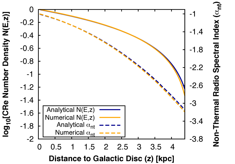
Figure 12: Profiles of the CRe number density at $\lambda$22 cm (equivalent to a CRe energy of $2.9$ GeV) for a constant magnetic field and advective cosmic ray transport ($B=10~{}\mu\rm G$, $U_{\rm rad}/U_{\rm B}=0.31$, $V=150~{}\rm km\,s^{-1}$, $\gamma_{\rm inj}=3.0$). Compared are the analytical and numerical solutions, which are plotted on the left-hand side $y$-axis. The corresponding non-thermal radio spectral indices between $\lambda\lambda$ 22 and 6 cm are plotted on the right-hand side $y$-axis.

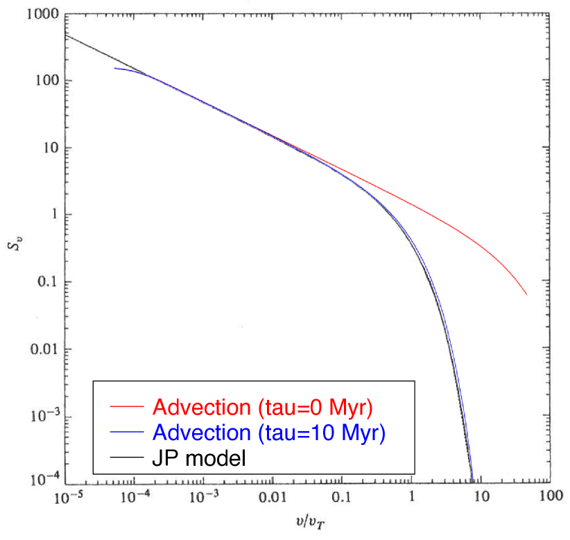
Figure 13: Comparison of our advection model with a JP spectrum taken from Hughes (1991). The upper, red line shows the injection spectrum ($\gamma_{\rm inj}=2.0$, $\tau=0$ Myr) and the lower, blue line shows the spectrally aged spectrum ($\tau=10$ Myr). The lower, black line shows the JP model to which our spectrum should be compared. The flux densities $S_{\nu}$ are on an arbitrary scale. The frequencies $\nu$ are normalized to the break frequency $\nu_{\rm T}=20.7$ GHz ($B=10~{}\mu\rm G$, $U_{\rm IRF}/U_{\rm B}=0$). IC losses in the CMB at redshift zero are taken into account.

Comparison with reference models

We can test the numerical solution of the advection equation for a constant magnetic field strength, for which there is an analytical solution for the CRe number distribution (e.g. Longair, 2011):

$$N(E,z)=N_{0}\left(1-\frac{bz}{E}\right)^{\gamma-1}.$$ (33)

In Fig. 12, we compare the analytical with the numerical solution. We find that the electron number densities agree to within 1 per cent at distances from the disc $z<3.0$ kpc, where the non-thermal spectral index is $\alpha_{\rm nt}>-2.2$. Even at larger distances where the spectral index steepens to a very steep $-3.0$, the agreement is better than 6 per cent. Since this is the regime we are mostly interested in, our numerical solution is of sufficient accuracy.

A second test is to compare our model with the widely used Jaffe–Perola (JP; Jaffe & Perola, 1973) model, which predicts a spectrum of the non-thermal radio continuum intensity as function of frequency. This model used the CRe number distribution of Equation (33) and convolves it with the synchrotron emission spectrum of a single CRe. In Fig. 13 we compare the synchrotron intensities from our modelling with the JP spectrum as presented in Hughes (1991). The upper, red line shows the injection spectrum and the lower, blue line the spectrally aged spectrum at a spectral age of 10 Myr. The theoretical predication by the JP model is shown as the lower, black line. The frequency is normalized with respect to the break frequency $\nu_{\rm brk}$ for which we find (e.g. Hughes, 1991):

$$\nu_{\rm T}=\frac{2.52\times 10^{3}[B/10~{}\mu{\rm G}]}{([B/10~{}\mu{\rm G}]^{2}+[B_{\rm CMB}/10~{}\mu{\rm G}]^{2})^{2}[\tau/\rm Myr]^{2}}~{}{\rm GHz}\mbox{.}$$ (34)

Here, the equivalent CMB magnetic field strength at redshift zero is $B_{\rm CMB}=3.2~{}\rm\mu G$. For our case ($B=10~{}\mu\rm G$, $U_{\rm IRF}=0$, $\tau=10$ Myr), the break frequency is $\nu_{\rm T}=20.7~{}\rm GHz$. At the break frequency the spectrally aged spectrum is deficient by a factor of four compared with the injection spectrum. We find a very good agreement between our spectrum and the reference spectrum from Hughes (1991).

Appendix B Data tables

In this appendix we present tables of the data used in the paper for the analysis. Tables 6 and 7 contain the non-thermal scale heights and CRe radiation lifetimes in NGC 7090 and 7462, respectively. Tables 8 and 9 contain the vertical profiles of the non-thermal radio spectral index in NGC 7090 and 7462, respectively. Quantities for the northern/southern haloes are designated as ‘N/S’. Finally, in Table 10 we present vertical profiles in NGC 7090 of the linearly polarized emission together, degrees of polarization together with the total ($B$), ordered ($B_{\rm ord}$) and turbulent ($B_{\rm turb}$) magnetic field strengths.

Table 6: Non-thermal radio continuum scale heights measured from two-component exponential fits and CRe radiation lifetimes in the northern (N) and southern (S) halo of NGC 7090.

Offset	Thin disc (kpc)				Thick disc (kpc)				Rad. lif. (Myr)
(kpc)	$\lambda$22 cm (N)	$\lambda$6 cm (N)	$\lambda$22 cm (S)	$\lambda$6 cm (S)	$\lambda$22 cm (N)	$\lambda$6 cm (N)	$\lambda$22 cm (S)	$\lambda$6 cm (S)	$t_{\rm rad22}$	$t_{\rm rad6}$
$-3.4$	$0.34\pm 0.08$	$0.31\pm 0.08$	$0.44\pm 0.05$	$0.23\pm 0.13$	$1.54\pm 0.35$	$1.18\pm 1.00$	$2.65\pm 1.85$	$0.92\pm 1.85$	$28.0\pm 2.0$	$15.3\pm 1.0$
$-1.7$	$0.41\pm 0.05$	$0.47\pm 0.09$	$0.39\pm 0.05$	$0.21\pm 0.08$	$1.57\pm 0.12$	$1.31\pm 0.89$	$2.17\pm 0.47$	$1.06\pm 0.47$	$20.5\pm 2.0$	$11.2\pm 1.0$
$0.0$	$0.31\pm 0.03$	$0.34\pm 0.05$	$0.38\pm 0.04$	$0.18\pm 0.12$	$1.92\pm 0.12$	$2.04\pm 0.48$	$1.52\pm 0.29$	$0.97\pm 0.29$	$17.2\pm 2.0$	$9.4\pm 1.0$
$1.7$	$0.34\pm 0.18$	$0.47\pm 0.15$	$0.50\pm 0.10$	$0.40\pm 0.07$	$1.67\pm 0.18$	$2.15\pm 0.55$	$1.40\pm 1.00$	$1.77\pm 1.00$	$21.0\pm 3.0$	$11.5\pm 1.0$
$3.4$	$0.63\pm 0.13$	$0.21\pm 0.99$	$0.04\pm 0.46$	$0.46\pm 0.25$	$2.33\pm 0.55$	$2.01\pm 1.19$	$1.35\pm 0.25$	$1.39\pm 0.25$	$26.0\pm 2.0$	$13.9\pm 1.0$

Table 7: Non-thermal radio continuum scale heights measured from one-component Gaussian fits and CRe radiation lifetimes in the northern (N) and southern (S) halo of NGC 7462.

	Thick disc (kpc)				Rad. lif. (Myr)
Offset (kpc)	$\lambda$22 cm (N)	$\lambda$6 cm (N)	$\lambda$22 cm (S)	$\lambda$6 cm (S)	$t_{\rm rad22}$	$t_{\rm rad6}$
$-4.8$	$2.17\pm 0.15$	$1.58\pm 0.08$	$1.96\pm 0.11$	$2.01\pm 0.13$	$29.5\pm 2.0$	$16.1\pm 1.0$
$-2.4$	$1.11\pm 0.15$	$1.11\pm 0.04$	$1.42\pm 0.05$	$1.34\pm 0.03$	$21.2\pm 2.0$	$11.6\pm 1.0$
$0.0$	$1.36\pm 0.07$	$1.23\pm 0.08$	$1.35\pm 0.04$	$1.32\pm 0.03$	$19.0\pm 2.0$	$10.4\pm 1.0$
$2.4$	$1.89\pm 0.09$	$2.27\pm 0.11$	$1.79\pm 0.05$	$1.61\pm 0.05$	$25.6\pm 2.0$	$14.0\pm 1.0$
$4.8$	$1.56\pm 0.09$	$1.94\pm 0.24$	$1.09\pm 0.06$	$1.41\pm 0.12$	$32.6\pm 2.0$	$17.8\pm 1.0$

Table 8: Vertical profiles of the non-thermal radio continuum intensities (at $\lambda\lambda$ 22 and 6 cm) and of the radio spectral index (between $\lambda\lambda$ 22 and 6 cm) in the northern (N) and southern (S) halo of NGC 7090.

$|z|$	$I_{\rm nt22}$ (N)	$I_{\rm nt6}$ (N)	$\alpha_{\rm nt}$ (N)	$I_{\rm nt22}$(S)	$I_{\rm nt6}$ (S)	$\alpha_{\rm nt}$ (S)
(kpc)	($\mu\rm Jy\,beam^{-1}$)			($\mu\rm Jy\,beam^{-1}$)
$0.1750$	$1266\pm 64$	$380\pm 19$	$-0.99\pm 0.07$	$1214\pm 61$	$336\pm 17$	$-1.06\pm 0.07$
$0.5250$	$922\pm 47$	$260\pm 13$	$-1.05\pm 0.07$	$836\pm 43$	$201\pm 11$	$-1.18\pm 0.07$
$0.8750$	$585\pm 30$	$150\pm 8$	$-1.12\pm 0.08$	$485\pm 26$	$102\pm 6$	$-1.29\pm 0.09$
$1.2250$	$378\pm 21$	$85\pm 6$	$-1.23\pm 0.10$	$277\pm 16$	$58\pm 5$	$-1.29\pm 0.11$
$1.5750$	$287\pm 16$	$54\pm 5$	$-1.37\pm 0.12$	$187\pm 12$	$39\pm 4$	$-1.30\pm 0.14$
$1.9250$	$249\pm 15$	$48\pm 4$	$-1.37\pm 0.13$	$148\pm 11$	$33\pm 4$	$-1.23\pm 0.16$
$2.2750$	$230\pm 14$	$49\pm 4$	$-1.28\pm 0.13$	$118\pm 10$	$32\pm 4$	$-1.07\pm 0.17$
$2.6250$	$189\pm 12$	$41\pm 4$	$-1.25\pm 0.14$	$78\pm 9$	$19\pm 4$	$-1.18\pm 0.24$
$2.9750$	$147\pm 11$	$32\pm 4$	$-1.25\pm 0.16$	$34\pm 8$	$1\pm 4$	$-3.17\pm 4.19$
$3.3250$	$122\pm 10$	$21\pm 4$	$-1.47\pm 0.21$	$32\pm 8$	$3\pm 4$	$-2.08\pm 1.24$
$3.6750$	$101\pm 9$	$15\pm 4$	$-1.60\pm 0.27$	$52\pm 8$	$10\pm 4$	$-1.36\pm 0.39$
$4.0250$	$85\pm 9$	$12\pm 4$	$-1.60\pm 0.31$	$59\pm 9$	$11\pm 4$	$-1.40\pm 0.36$

Table 9: Vertical profiles of the non-thermal radio continuum intensities (at $\lambda\lambda$ 22 and 6 cm) and of the radio spectral index (between $\lambda\lambda$ 22 and 6 cm) in the northern (N) and southern (S) halo of NGC 7462.

$|z|$	$I_{\rm nt22}$ (N)	$I_{\rm nt6}$ (N)	$\alpha_{\rm nt}$ (N)	$I_{\rm nt22}$(S)	$I_{\rm nt6}$ (S)	$\alpha_{\rm nt}$ (S)
(kpc)	($\mu\rm Jy\,beam^{-1}$)			($\mu\rm Jy\,beam^{-1}$)
$0.225$	$638\pm 33$	$142\pm 8$	$-1.24\pm 0.06$	$716\pm 36$	$157\pm 8$	$-1.25\pm 0.06$
$0.675$	$468\pm 24$	$109\pm 6$	$-1.20\pm 0.06$	$581\pm 30$	$132\pm 7$	$-1.22\pm 0.06$
$1.125$	$302\pm 17$	$76\pm 5$	$-1.14\pm 0.07$	$400\pm 21$	$98\pm 5$	$-1.16\pm 0.06$
$1.575$	$182\pm 11$	$45\pm 3$	$-1.16\pm 0.08$	$243\pm 14$	$57\pm 4$	$-1.20\pm 0.07$
$2.025$	$107\pm 9$	$21\pm 3$	$-1.33\pm 0.13$	$144\pm 10$	$30\pm 3$	$-1.30\pm 0.10$
$2.475$	$79\pm 8$	$11\pm 3$	$-1.66\pm 0.22$	$67\pm 8$	$14\pm 3$	$-1.28\pm 0.18$
$2.925$	$66\pm 8$	$5\pm 3$	$-2.19\pm 0.46$	$25\pm 7$	$4\pm 3$	$-1.49\pm 0.54$
$3.375$	$39\pm 7$	$3\pm 3$	$-2.25\pm 0.82$	$19\pm 7$	$2\pm 3$	$-1.92\pm 1.12$

Table 10: Vertical profiles of the linearly polarized intensity, degree of polarization (at $\lambda\lambda$ 22 and 6 cm, respectively) and magnetic field strengths in NGC 7090. Positive values of $z$ denote the northern and negative ones the southern halo.

$z$	$PI_{22}$	$PI_{6}$	$p_{22}$	$p_{6}$	$\alpha_{\rm nt}$	$B$	$B_{\rm ord}$	$B_{\rm turb}$
(kpc)	($\mu\rm Jy\,beam^{-1}$)	($\mu\rm Jy\,beam^{-1}$)				($\mu\rm G$)	($\mu\rm G$)	($\mu\rm G$)
$-6.65$	$13\pm 11$	$4\pm 5$	$0.12\pm 0.13$	$-$	$-$	$0.70\pm 0.24$	$0.26\pm 0.25$	$0.65\pm 0.28$
$-5.95$	$30\pm 11$	$9\pm 5$	$0.27\pm 0.18$	$-$	$-3.55\pm 15.55$	$0.83\pm 0.26$	$0.46\pm 0.24$	$0.69\pm 0.36$
$-5.25$	$31\pm 11$	$10\pm 5$	$0.21\pm 0.12$	$0.81\pm 1.90$	$-2.01\pm 1.92$	$0.99\pm 0.29$	$0.51\pm 0.23$	$0.85\pm 0.36$
$-4.55$	$34\pm 11$	$2\pm 5$	$0.17\pm 0.08$	$0.06\pm 0.19$	$-1.67\pm 0.92$	$1.18\pm 0.32$	$0.54\pm 0.20$	$1.05\pm 0.37$
$-3.85$	$55\pm 12$	$12\pm 5$	$0.24\pm 0.08$	$0.34\pm 0.33$	$-1.59\pm 0.75$	$1.41\pm 0.34$	$0.76\pm 0.24$	$1.18\pm 0.44$
$-3.15$	$73\pm 12$	$20\pm 5$	$0.26\pm 0.07$	$0.41\pm 0.26$	$-1.43\pm 0.53$	$1.67\pm 0.37$	$1.21\pm 0.33$	$1.16\pm 0.64$
$-2.45$	$80\pm 12$	$30\pm 5$	$0.16\pm 0.03$	$0.27\pm 0.09$	$-1.25\pm 0.24$	$1.99\pm 0.40$	$1.18\pm 0.32$	$1.61\pm 0.55$
$-1.75$	$73\pm 12$	$39\pm 5$	$0.07\pm 0.01$	$0.16\pm 0.03$	$-1.24\pm 0.12$	$2.38\pm 0.42$	$1.08\pm 0.23$	$2.12\pm 0.49$
$-1.05$	$47\pm 12$	$41\pm 5$	$0.02\pm 0.00$	$0.07\pm 0.01$	$-1.17\pm 0.07$	$2.83\pm 0.45$	$0.86\pm 0.16$	$2.70\pm 0.47$
$-0.35$	$33\pm 11$	$25\pm 5$	$0.01\pm 0.00$	$0.02\pm 0.00$	$-1.09\pm 0.06$	$6.46\pm 0.36$	$1.13\pm 0.16$	$6.36\pm 0.36$
$0.35$	$28\pm 11$	$14\pm 5$	$0.01\pm 0.00$	$0.01\pm 0.00$	$-1.06\pm 0.06$	$6.46\pm 0.36$	$0.81\pm 0.18$	$6.41\pm 0.36$
$1.05$	$23\pm 11$	$32\pm 5$	$0.01\pm 0.00$	$0.04\pm 0.01$	$-1.11\pm 0.07$	$2.84\pm 0.45$	$0.68\pm 0.13$	$2.76\pm 0.46$
$1.75$	$30\pm 11$	$37\pm 5$	$0.02\pm 0.01$	$0.10\pm 0.02$	$-1.24\pm 0.10$	$2.50\pm 0.47$	$0.92\pm 0.20$	$2.32\pm 0.51$
$2.45$	$52\pm 12$	$31\pm 5$	$0.05\pm 0.01$	$0.15\pm 0.03$	$-1.30\pm 0.14$	$2.20\pm 0.47$	$0.96\pm 0.24$	$1.98\pm 0.54$
$3.15$	$96\pm 12$	$22\pm 5$	$0.14\pm 0.02$	$0.17\pm 0.05$	$-1.34\pm 0.20$	$1.94\pm 0.47$	$0.90\pm 0.23$	$1.72\pm 0.54$
$3.85$	$108\pm 13$	$13\pm 5$	$0.25\pm 0.05$	$0.15\pm 0.08$	$-1.35\pm 0.31$	$1.71\pm 0.46$	$0.96\pm 0.28$	$1.41\pm 0.59$
$4.55$	$92\pm 12$	$4\pm 5$	$0.37\pm 0.11$	$0.06\pm 0.07$	$-1.01\pm 0.39$	$1.50\pm 0.44$	$1.06\pm 0.36$	$1.07\pm 0.72$
$5.25$	$74\pm 12$	$7\pm 5$	$0.54\pm 0.26$	$0.12\pm 0.11$	$-0.72\pm 0.56$	$1.32\pm 0.43$	$1.14\pm 0.50$	$0.66\pm 1.21$
$5.95$	$66\pm 12$	$13\pm 5$	$0.55\pm 0.30$	$1.00\pm 2.32$	$-1.85\pm 1.93$	$1.16\pm 0.41$	$0.96\pm 0.46$	$0.66\pm 0.99$
$6.65$	$31\pm 11$	$9\pm 5$	$0.26\pm 0.17$	$-$	$-$	$1.03\pm 0.39$	$0.58\pm 0.32$	$0.85\pm 0.52$

References

- Adebahr et al. (2013) Adebahr B., Krause M., Klein U., Weżgowiec M., Bomans D. J., Dettmar R.-J., 2013, A&A, 555, A23
- Arribas et al. (2014) Arribas S., Colina L., Bellocchi E., Maiolino R., Villar-Martín M., 2014, A&A, 568, A14
- Baars et al. (1977) Baars J. W. M., Genzel R., Pauliny-Toth I. I. K., Witzel A., 1977, A&A, 61, 99
- Beck & Krause (2005) Beck R., Krause M., 2005, Astron. Nachr., 326, 414
- Berkhuijsen et al. (2013) Berkhuijsen E. M., Beck R., Tabatabaei F. S., 2013, MNRAS, 435, 1598
- Boettcher et al. (2013) Boettcher E., Zweibel E. G., Yoast-Hull T. M., Gallagher III J. S., 2013, ApJ, 779, 12
- Braun et al. (2010) Braun R., Heald G., Beck R., 2010, A&A, 514, A42
- Bregman (1980) Bregman J. N., 1980, ApJ, 236, 577
- Breitschwerdt et al. (1991) Breitschwerdt D., McKenzie J. F., Völk H. J., 1991, A&A, 245, 79
- Breitschwerdt et al. (1993) Breitschwerdt D., McKenzie J. F., Völk H. J., 1993, A&A, 269, 54
- Buffie et al. (2013) Buffie K., Heesen V., Shalchi A., 2013, ApJ, 764, 37
- Burn (1966) Burn B. J., 1966, MNRAS, 133, 67
- Condon (1992) Condon J. J., 1992, ARA&A, 30, 575
- Dahlem et al. (1997) Dahlem M., Petr M. G., Lehnert M. D., Heckman T. M., Ehle M., 1997, A&A, 320, 731
- Dahlem et al. (2001) Dahlem M., Ehle M., Ryder S. D., 2001, A&A, 373, 485
- Dahlem et al. (2005) Dahlem M., Ehle M., Ryder S. D., Vlajić M., Haynes R. F., 2005, A&A, 432, 475
- Dahlem et al. (2006) Dahlem M., Lisenfeld U., Rossa J., 2006, A&A, 457, 121
- Dale & Helou (2002) Dale D. A., Helou G., 2002, ApJ, 576, 159
- Dale et al. (2009) Dale D. A., et al., 2009, ApJ, 703, 517
- Dalla Vecchia & Schaye (2008) Dalla Vecchia C., Schaye J., 2008, MNRAS, 387, 1431
- Deeg et al. (1997) Deeg H.-J., Duric N., Brinks E., 1997, A&A, 323, 323
- Dettmar (1992) Dettmar R.-J., 1992, Fundamentals Cosmic Phys., 15, 143
- Dorfi & Breitschwerdt (2012) Dorfi E. A., Breitschwerdt D., 2012, A&A, 540, A77
- Doyle et al. (2005) Doyle M. T., et al., 2005, MNRAS, 361, 34
- Draine (2011) Draine B. T., 2011, Physics of the Interstellar and Intergalactic Medium. Princeton University Press, Princeton, NJ
- Dumke et al. (1995) Dumke M., Krause M., Wielebinski R., Klein U., 1995, A&A, 302, 691
- Ekers & Sancisi (1977) Ekers R. D., Sancisi R., 1977, A&A, 54, 973
- Everett et al. (2008) Everett J. E., Zweibel E. G., Benjamin R. A., McCammon D., Rocks L., Gallagher III J. S., 2008, ApJ, 674, 258
- Ferrière (2001) Ferrière K. M., 2001, Reviews of Modern Physics, 73, 1031
- Fletcher et al. (2011) Fletcher A., Beck R., Shukurov A., Berkhuijsen E. M., Horellou C., 2011, MNRAS, 412, 2396
- Hanasz et al. (2009) Hanasz M., Wóltański D., Kowalik K., 2009, ApJ, 706, L155
- Heesen et al. (2009a) Heesen V., Beck R., Krause M., Dettmar R.-J., 2009a, A&A, 494, 563
- Heesen et al. (2009b) Heesen V., Krause M., Beck R., Dettmar R.-J., 2009b, A&A, 506, 1123
- Heesen et al. (2011) Heesen V., Beck R., Krause M., Dettmar R.-J., 2011, A&A, 535, A79
- Heesen et al. (2014) Heesen V., Brinks E., Leroy A. K., Heald G., Braun R., Bigiel F., Beck R., 2014, AJ, 147, 103
- Heesen et al. (2015) Heesen V., et al., 2015, MNRAS, 447, L1
- Hodges-Kluck & Bregman (2013) Hodges-Kluck E. J., Bregman J. N., 2013, ApJ, 762, 12
- Hodges-Kluck & Bregman (2014) Hodges-Kluck E. J., Bregman J. N., 2014, ApJ, 789, 131
- Hughes (1991) Hughes P. A., 1991, Beams and Jets in Astrophysics. Cambridge University Press, Cambridge, UK
- Hughes et al. (2014) Hughes T. M., et al., 2014, A&A, 565, A4
- Hummel et al. (1988) Hummel E., Lesch H., Wielebinski R., Schlickeiser R., 1988, A&A, 197, L29
- Hunter et al. (2012) Hunter D. A., et al., 2012, AJ, 144, 134
- Ipavich (1975) Ipavich F. M., 1975, ApJ, 196, 107
- Irwin et al. (1999) Irwin J. A., English J., Sorathia B., 1999, AJ, 117, 2102
- Irwin et al. (2012) Irwin J., et al., 2012, AJ, 144, 43
- Jaffe & Perola (1973) Jaffe W. J., Perola G. C., 1973, A&A, 26, 423
- Karachentsev et al. (2013) Karachentsev I. D., Makarov D. I., Kaisina E. I., 2013, AJ, 145, 101
- Kennicutt et al. (2008) Kennicutt Jr. R. C., Lee J. C., Funes José G. S. J., Sakai S., Akiyama S., 2008, ApJS, 178, 247
- Kepley et al. (2010) Kepley A. A., Mühle S., Everett J., Zweibel E. G., Wilcots E. M., Klein U., 2010, ApJ, 712, 536
- Krause (2009) Krause M., 2009, Rev. Mex. Astron. Astrofis., 36, 25
- Krause (2011) Krause M., 2011, in Proceedings of ‘Magnetic Fields in the Universe: From Laboratory and Stars to Primordial Structures’, eds. M. Soida, K. Otmianowska-Mazur, E.M. de Gouveia Dal Pino & A. Lazarian. (arXiv:1111.7081)
- Krause et al. (2006) Krause M., Wielebinski R., Dumke M., 2006, A&A, 448, 133
- Kulsrud & Pearce (1969) Kulsrud R., Pearce W. P., 1969, ApJ, 156, 445
- Lisenfeld & Völk (2000) Lisenfeld U., Völk H. J., 2000, A&A, 354, 423
- Longair (2011) Longair M. S., 2011, High Energy Astrophysics. Cambridge University Press, Cambridge, UK
- Mao et al. (2015) Mao S. A., Zweibel E., Fletcher A., Ott J., Tabatabaei F., 2015, ApJ, 800, 92
- Marvil et al. (2015) Marvil J., Owen F., Eilek J., 2015, AJ, 149, 32
- McMullin et al. (2007) McMullin J. P., Waters B., Schiebel D., Young W., Golap K., 2007, ASP Conf. Ser., 376, 127
- Mora & Krause (2013) Mora S. C., Krause M., 2013, A&A, 560, A42
- Moss et al. (2010) Moss D., Sokoloff D., Beck R., Krause M., 2010, A&A, 512, A61
- Mulcahy et al. (2014) Mulcahy D. D., et al., 2014, A&A, 568, A74
- Murphy et al. (2008) Murphy E. J., Helou G., Kenney J. D. P., Armus L., Braun R., 2008, ApJ, 678, 828
- Neininger & Dumke (1999) Neininger N., Dumke M., 1999, Proc. Natl. Acad. Sci. USA, 96, 5360
- Niklas & Beck (1997) Niklas S., Beck R., 1997, A&A, 320, 54
- Niklas et al. (1997) Niklas S., Klein U., Wielebinski R., 1997, A&A, 322, 19
- Oosterloo et al. (2007) Oosterloo T., Fraternali F., Sancisi R., 2007, AJ, 134, 1019
- Press et al. (1992) Press W. H., Teukolsky S. A., Vetterling W. T., Flannery B. P., 1992, Numerical recipes in FORTRAN. The Art of Scientific Computing. Cambridge University Press, Cambridge, UK
- Rau & Cornwell (2011) Rau U., Cornwell T. J., 2011, A&A, 532, A71
- Rohlfs & Wilson (2004) Rohlfs K., Wilson T. L., 2004, Tools of Radio Astronomy. Springer, Berlin, Germany
- Rossa & Dettmar (2003a) Rossa J., Dettmar R.-J., 2003a, A&A, 406, 493
- Rossa & Dettmar (2003b) Rossa J., Dettmar R.-J., 2003b, A&A, 406, 505
- Rossa et al. (2004) Rossa J., Dettmar R.-J., Walterbos R. A. M., Norman C. A., 2004, AJ, 128, 674
- Sault et al. (1995) Sault R. J., Teuben P. J., Wright M. C. H., 1995, ASP Conf. Ser., 77, 433
- Schlafly & Finkbeiner (2011) Schlafly E. F., Finkbeiner D. P., 2011, ApJ, 737, 103
- Shapiro & Field (1976) Shapiro P. R., Field G. B., 1976, ApJ, 205, 762
- Soida et al. (2011) Soida M., Krause M., Dettmar R.-J., Urbanik M., 2011, A&A, 531, A127
- Sokoloff et al. (1998) Sokoloff D. D., Bykov A. A., Shukurov A., Berkhuijsen E. M., Beck R., Poezd A. D., 1998, MNRAS, 299, 189
- Strong et al. (2007) Strong A. W., Moskalenko I. V., Ptuskin V. S., 2007, Annu. Rev. Nucl. Part. Sci., 57, 285
- Tabatabaei et al. (2013a) Tabatabaei F. S., et al., 2013a, A&A, 552, A19
- Tabatabaei et al. (2013b) Tabatabaei F. S., Berkhuijsen E. M., Frick P., Beck R., Schinnerer E., 2013b, A&A, 557, A129
- Tüllmann et al. (2000) Tüllmann R., Dettmar R.-J., Soida M., Urbanik M., Rossa J., 2000, A&A, 364, L36
- Tüllmann et al. (2006) Tüllmann R., Pietsch W., Rossa J., Breitschwerdt D., Dettmar R.-J., 2006, A&A, 448, 43
- Völk (1989) Völk H. J., 1989, A&A, 218, 67
- Wiegert et al. (2015) Wiegert T., et al., 2015, AJ, 150, 81
- van Haarlem et al. (2013) van Haarlem M. P., et al., 2013, A&A, 556, A2