Parallel Shortest-Paths Using Radius Stepping

Abstract

The single-source shortest path problem (Sssp) with nonnegative edge weights is a notoriously difficult problem to solve efficiently in parallel—it is one of the graph problems said to suffer from the transitive-closure bottleneck. In practice, the $\Delta$-stepping algorithm of Meyer and Sanders (J. Algorithms, 2003) often works efficiently but has no known theoretical bounds on general graphs. The algorithm takes a sequence of steps, each increasing the radius by a user-specified value $\Delta$. Each step settles the vertices in its annulus but can take $\Theta(n)$ substeps, each requiring $\Theta(m)$ work ($n$ vertices and $m$ edges).

In this paper, we describe Radius-Stepping, an algorithm with the best-known tradeoff between work and depth bounds for Sssp with nearly-linear ($\widetilde{O}(m)$) work. The algorithm is a $\Delta$-stepping-like algorithm but uses a variable instead of fixed-size increase in radii, allowing us to prove a bound on the number of steps. In particular, by using what we define as a vertex $k$-radius, each step takes at most $k+2$ substeps. Furthermore, we define a $(k,\rho)$-graph property and show that if an undirected graph has this property, then the number of steps can be bounded by $O(\frac{n}{\rho}\log\rho L)$, for a total of $O(\frac{kn}{\rho}\log\rho L)$ substeps, each parallel. We describe how to preprocess a graph to have this property. Altogether, Radius-Stepping takes $O(m\log n)$ work and $O(\frac{n}{\rho}\log n\log(\rho{}L))$ depth per source after preprocessing. The preprocessing step can be done in $O(m\log n+n\rho^{2})$ work and $O(\rho^{2})$ depth or in $O(m\log n+n\rho^{2}\log n)$ work and $O(\rho\log\rho)$ depth, and adds no more than $O(n\rho)$ edges.

1 Introduction

The single-source shortest path problem (Sssp) is a fundamental graph problem that is extremely well-studied and has numerous practical and theoretical applications. For a weighted graph $G=(V,E,w)$ with $n=|V|$ vertices and $m=|E|$ edges, and a source node $s\in V$, the Sssp problem with nonnegative edge weights is to find the shortest (i.e., minimum weight) path from $s$ to every $v\in V$, according to the weight function $w\!:E\to\mathbb{R}_{+}$, which assigns to every edge a real-valued nonnegative weight (“distance”). We will assume without loss of generality that the lightest nonzero edge has weight $1$, i.e, $\min_{e:w(e)>0}w(e)=1$. Let $L=\max_{e}w(e)$.

In the sequential setting, Dijkstra’s algorithm [8] solves this problem in $O(m+n\log n)$ time using the Fibonacci heap [10]. This is the best theoretical running time for general nonnegative edge weights although faster algorithms exist for certain special cases. Thorup [26], for example, gives an $O(m+n)$-time algorithm for when the edge weights are positive integers.

In the parallel setting, the holy grail of parallel Sssp is an algorithm with Dijkstra’s work bound (i.e., work-efficient) that runs in small depth. Although tens of algorithms for the problem have been proposed over the last several decades, none of the existing algorithms that take the same amount of work as Dijkstra’s have polylogarithmic or even $o(n)$ depth. This has led Karp and Ramachandran to coin the term transitive closure bottleneck [14]. We survey existing algorithms most relevant to this work in Section 6.

Apart from the quest for a polylogarithmic-depth, work-efficient algorithm, one could aim for an algorithm with a high degree of parallelism ($\mathbb{P}=W/D$) that is work-efficient or nearly work-efficient. From a performance point of view, both factors are important because work efficiency is a prerequisite for the algorithm to quickly gain speedups over the sequential algorithm, and the parallelism factor $\mathbb{P}$ indicates how well the algorithm will scale with processors.

This observation has fueled the design of Sssp algorithms with substantial parallelism that are nearly work-efficient. Spencer [25] shows that BFS can be solved in $O(\frac{n}{\rho}\log^{2}\rho)$ depth and $O((m+n\rho^{2}\log\rho)\log\rho)$ work, where $\sqrt{m/n}\leq\rho$ is a tuneable parameter. On a weighted graph, Sssp requires $O(\frac{n}{\rho}\log n\log(\rho{}L))$ depth and $O((n\rho^{2}\log\rho+m)\log(n\rho L))$ work, where $\log({\rho{}L})\leq\rho$. At a high-level, these algorithms use limited path-doubling to determine the shortest-path distances to about $\rho$ vertices in each round, requiring slightly more than $\tfrac{n}{\rho}$ rounds in total.

On the empirical side, the $\Delta$-stepping algorithm of Meyer and Sanders [18] works well on many kinds of graphs. The algorithm has been analyzed for random graphs, but no theoretical guarantees are known for the general case. $\Delta$-stepping is a hybrid of Dijkstra’s algorithm and the Bellman-Ford algorithm. It determines the correct distances from $s$ in increments of $\Delta$, settling in step $i$ all the vertices whose shortest-path distances are between $i\Delta$ and $(i+1)\Delta$. Within each step, the algorithm resorts to running Bellman-Ford as substeps to determine the distances to such vertices. Altogether, the algorithm performs up to a total of $\frac{LK}{\Delta}$ rounds of substeps, where $K$ the shortest-path distance to the farthest vertex from $s$.

Our Contributions: In this paper, we investigate the single-source shortest-path problem for weighted, undirected graphs. The main result is as follows:

Theorem 1.1.

Let $G$ be an undirected, weighted graph with $n$ vertices and $m$ edges. For $\rho\leq\sqrt{n}$, there is an algorithm, Radius-Stepping, that after a preprocessing phase can solve Sssp from any source in $O(m\log n)$ work and $O(\frac{n}{\rho}\log n\log{\rho{}L})$ depth. In addition, the preprocessing phase takes $O(m\log n+n\rho^{2})$ work and $O(\rho^{2})$ depth, or $O(m\log n+n\rho^{2}\log n)$ work and $O(\rho\log\rho)$ depth.

Compared to a standard Dijkstra’s implementation, the algorithm, excluding preprocessing, is work-efficient up to only a $\log n$ factor. Using $\rho=\mathrm{polylog}(n)$, the algorithm offers at least polylogarithmic parallelism. Using $\rho=n^{O(\varepsilon)}$, the algorithm has sublinear depth. As far as we know, this is the best tradeoff between work and depth for the problem.

Our algorithm Radius-Stepping (Section 3) can be seen as a hybrid variant of $\Delta$-stepping and Spencer’s algorithm, though simpler. Like $\Delta$-stepping, it performs Dijkstra’s-like steps in the outer loop, finding and settling multiple vertices at a time using (restricted) Bellman-Ford as substeps. Unlike $\Delta$-stepping, however, the algorithm judiciously picks a new step size ($\Delta$) every time. The step size is chosen so that, like in Spencer’s algorithm, about $\rho$ new vertices are settled in every step, or otherwise it doubles the distance explored. Yet, unlike Spencer’s algorithm, Radius-Stepping does not perform path doubling in every iteration, leading to a conceptually simpler algorithm with fewer moving parts. Ultimately, the steps of Radius-Stepping parallel Dijkstra’s execution steps, and the only invariant necessary is a natural generalization of Dijkstra’s invariant.

We prove that Radius-Stepping runs in $O(\tfrac{n}{\rho}\log(\rho{}L))$ steps, each running up to $O(k)$ substeps, provided that the input graph is a $(k,\rho)$-graph. This is informally defined to be a graph in which every node can reach its $\rho$ closest vertices within $k$ hops. We show how to implement this algorithm in $O(km\log n)$ work and $O(k\frac{n}{\rho}\log n\log{\rho{}L})$ depth. For unweighted graphs, it can be implemented in $O(k(m+n))$ work and $O(k\frac{n}{\rho}\log\rho\log^{*}\rho)$ depth.

However, not all graphs are $(k,\rho)$-graphs as given, but, as will be discussed in Section 4, they can be made so with a preprocessing step that runs restricted Dijkstra’s to discover the $\rho$ closest vertices for all vertices in parallel. To make the graph a $(1,\rho)$-graph, the preprocessing step effectively adds up to $n\rho$ shortcut edges to the input graph. The number of shortcut edges can be reduced if we use a larger $k$. Although this saves some memory, Radius-Stepping will have to do slightly more work when computing the shortest paths. For $k>1$, it is less trivial to generate a $(k,\rho)$-graph that adds only a small number of edges. We present some heuristics in Section 4 and empirically study their quality in Section 5.

Our experiments aim to study the number of edges added by preprocessing and the number of steps taken by Radius-Stepping. This is a good proxy for measuring the depth of the algorithm experimentally. The results confirm our theory: the number of steps taken (that is, roughly the depth) is inversely proportional to $\rho$ for both the weighted and unweighted cases. They further show that with an appropriate heuristic (such as the dynamic programming heuristic from Section 4.2) and choice of parameters, preprocessing will add a reasonable number of edges (at most $O(m)$), thereby increasing the total work by at most a constant.

2 Preliminaries

Let $G=(V,E,w)$ be an undirected, simple, weighted graph. We assume without loss of generality that $G$ is a connected, simple graph (i.e., no self-loops nor parallel edges). For $S\subseteq V$, define $N(S)=\cup_{u\in S}\{v\,|\,(u,v)\in E\}$ to be the neighbor set of $S$. During the execution of standard breadth-first search (BFS) or Dijkstra’s algorithm, the frontier is the neighbor set of all visited vertices. Let $d(u,v)$ denote the shortest-path distance in $G$ between two vertices $u$ and $v$. The enclosed ball of a vertex $u$ is $B(u,r)=\{v\in V\,|\,d(u,v)\leq r\}$.

A shortest-path tree rooted at vertex $u$ is a spanning tree $T$ of $G$ (subtree if $G$ is unconnected) such that the path distance from the root $u$ to any other vertex $v\in T$ is the shortest-path distance from $v$ to $u$ in $G$. We say a graph is unweighted if $w(e)=1$ for all $e\in E$ (so $L=1$).

We assume the standard PRAM model that allows for concurrent reads and writes, and analyze the performance of our parallel algorithms in terms of work and depth [13], where work $W$ is equal to the total number of operations performed and depth (span) $D$ is equal to the longest sequence of dependent operations. Nonetheless, all of our algorithms can also be implemented on machines with exclusive writes. We say that an algorithm is work efficient if it performs the same amount of work as the best sequential counterpart, up to constants.

Consider two ordered sets $A$ and $B$ stored in balanced BSTs such that $|A|\leq|B|$. Recent research work shows that set union and set difference operations can be computed either in $O(|A|\log|B|)$ work and $O(\log|B|)$ depth [23, 21, 22], or in $O(|A|\log|B|/|A|)$ work and $O(\log|A|\log|B|)$ depth [3, 2]. In this paper we assume both set union and difference can be done in $O(|A|\log|B|)$ work and $O(\log|B|)$ depth.

Finally, we need a few definitions:

Definition 1 (Hop Distance).

Let $\hat{d}(u,v)$ be the number of edges on the shortest (weighted) path between $u$ and $v$ that uses the fewest edges.

Definition 2 ($k$-radius).

For $u\in V$, the $k$-radius of $u$, denoted by $\bar{r}_{k}(u)$, is $\min_{v\in V,\hat{d}(u,v)>k}{d(u,v)}$—that is, the closest distance to $u$ which is more than $k$ hops away.

3 The Radius-Stepping Algorithm

Input: A graph $G=(V,E,w)$, vertex radii $r(\cdot)$, and a source node $s$.

Output: The graph distances $\delta(\cdot)$ from $s$.

1 $\delta(\cdot)\leftarrow+\infty$, $\delta(s)\leftarrow 0$

2 foreach $v\in N(s)$ do $\delta(v)\leftarrow w(s,v)$

3 $S_{0}\leftarrow\{s\}$, $i\leftarrow 1$

4 while $|S_{i-1}|<|V|$ do

5       $d_{i}\leftarrow\min_{v\in V\setminus S_{i-1}}\{\delta(v)+r(v)\}$

6       repeat

7             foreach $u\in V\setminus S_{i-1}~{}s.t.~{}\delta(u)\leq d_{i}$ do

8                   foreach $v\in N(u)\setminus S_{i-1}$ do

9                         $\delta(v)\leftarrow\min\{\delta(v),\delta(u)+w(u,v)\}$

10                        

11      until no $\delta(v)\leq d_{i}$ was updated

12       $S_{i}=\{v\,|\,\delta(v)\leq d_{i}\}$

13       $i=i+1$

14      

return $\delta(\cdot)$

Algorithm 1 The Radius-Stepping Algorithm.

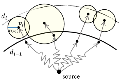
Figure 1: Illustration of a step of Algorithm 1: For all vertices whose neighbors are within $d_{i}$, we pick the node $v_{i}$, the lead node in the $i$-th round, that minimizes the tentative distance plus the vertex radius of this node. The round distance $d_{i}$ is set to $\delta(v_{i})+r(v_{i})$.

This section describes our algorithm for parallel Sssp called Radius-Stepping and discusses its performance analysis. We begin with a high-level description, which we analyze for the number of steps. Following that, we give a detailed implementation, which we analyze for work and depth.

The Radius-Stepping algorithm is presented in Algorithm 1. In broad strokes, it works as follows: The input to the algorithm is a weighted, undirected graph, a source vertex, and a target radius value for every vertex, given as a function $r\!:V\to\mathbb{R}_{+}$. The algorithm has the same basic structure as the $\Delta$-stepping algorithm; both are effectively a hybrid of Dijkstra’s algorithm and the Bellman-Ford algorithm. Like Dijkstra’s algorithm, they visit vertices in increasing distance from the source $s$, settling each vertex $v$—i.e., determining its correct distance $d(s,v)$. However, instead of visiting one vertex at a time, the algorithms visit nodes in steps (the while loop in Line 2-1). On each step $i$, the Radius-Stepping increments the radius centered at $s$ from $d_{i-1}$ to $d_{i}$, and settles all vertices $v$ in the annulus $d_{i-1}<d(s,v)\leq d_{i}$. This is illustrated in Figure 1.

Settling these vertices involves multiple substeps (the do loop in Lines 1–1) of what is effectively Bellman-Ford’s algorithm. Each substep is easily parallelized. In $\Delta$-stepping, the round distance $d_{i}=d_{i-1}+\Delta$ increases the radius by a fixed amount on each step. In the worst case, this can require $\Theta(n)$ substeps. This is not efficient since each substep will process the same set of vertices and their edges. In the worst case, it could take $O(nm)$ work.

In the Radius-Stepping algorithm, a new round distance $d_{i}$ is decided on each round with the goal of bounding the number of substeps. The algorithm takes a radius $r(v)$ for each vertex and selects a $d_{i}$ on step $i$ by taking the minimum of $\delta(v)+r(v)$ over all $v$ in the frontier (Line 1). Lines 1–1 then run the Bellman-Ford substeps until all vertices with radius less than $d_{i}$ are settled. Vertices within $d_{i}$ are then added to the visited set $S_{i}$.

The algorithm is correct for any radii $r(\cdot)$, but by setting it appropriately, it can be used to control the number of substeps per step and the number of steps. If $r(v)=0$, then the algorithm is effectively Dijkstra’s, and the inner step is run only once. It may, however, visit multiple vertices with the same distance. If $r(v)=\infty$, then the algorithm is effectively the Bellman-Ford algorithm, and the substeps will run until all vertices are settled, and hence there will be a single step. If $r(v)=\Delta$, then the algorithm is almost $\Delta$-stepping, but not quite since $\Delta$ is added to the distance of the nearest frontier vertex instead of to $d_{i-1}$.

In this paper, we aim to set $r(v)$ to be close, but no more, than the $k$-radius $\bar{r}_{k}(v)$. By making $r(v)$ no more than the $k$-radius, it guarantees that the algorithm will run at most $(k+2)$ Bellman-Ford substeps. For our theoretical bounds, we set $k=1$ so the algorithm only does constant substeps.

In addition to bounding the number of substeps, we want to bound the number of steps. To do this, we can make use of properties of the input graph. In particular if every vertex $v$ has $\rho$ vertices that are within a distance $r(v)$, i.e. $|B(v,r(v))|\geq\rho$, then we can bound the number of steps by $O(\tfrac{n}{\rho}\log(\rho L))$, where $L$ is the longest edge in the graph.

We will now prove the bound for the number of steps and substeps, then discuss the implementation details of Algorithm 1 in Section 3.3. In the analysis, we define the lead node in step $i$ as the node $v$ that attains $d_{i}$ in Line 1 and denote it by $v_{i}$.

Theorem 3.1 (Correctness).

After the $i$-th step of Radius-Stepping, each vertex $v$ with $d_{i-1}<d(s,v)\leq d_{i}$ will have $\delta(v)=d(s,v)$ and will be included in $S_{i}$.

Correctness of the algorithm is straightforward since it is essentially the $\Delta$-stepping algorithm with a variable step size: At the end of the inner loop, all vertices within the round distance are settled, and all of their direct neighbors are relaxed. Now we analyze the parallelism of this algorithm by bounding the longest chain of dependencies (depth).

Theorem 3.2 (The number of substeps).

The repeat-until loop (Lines 1–1) runs at most $k+2$ times provided that $r(v)\leq\bar{r}_{k}(v)$ for all $v\in V$.

Theorem 3.3 (The number of steps).

The while loop (Lines 2–1) requires no more than

$$\mathopen{}\mathclose{{}\left\lceil\frac{n}{\rho}}\right\rceil\mathopen{}\mathclose{{}\left(1+\lceil\log_{2}\rho L\rceil}\right)=O\mathopen{}\mathclose{{}\left(\frac{n}{\rho}\log(\rho L)}\right)$$

steps provided that $|B(v,r(v))|\geq\rho$ for all $v\in V$.

We prove these theorems in Sections 3.1 and 3.2.

3.1 Number of Substeps

Let $k$ be such that $r(v)\leq{\bar{r}_{k}({v})}$ for all $v\in V$. To bound the number of substeps, we use the fact that vertices with distances no more than the round distance in the previous round $(d_{i-1})$ are all correctly computed, as given by Theorem 3.1. Observe that their neighbors are also relaxed, since the distances to none of these vertices are updated in the last substep of the previous step (the termination condition in Line 1).

Lemma 3.4.

For a vertex $v\in V$, if $d_{i-1}<d(s,v)\leq d_{i}$, then its distance is correctly computed after $k+1$ substeps of the $i$-th step, i.e. $\delta(v)=d(s,v)$.

Proof.

Consider the shortest path from $s$ to $v$ that uses the fewest hops. Let $u$ be the first vertex on this path with distance larger than $d_{i-1}$. By Theorem 3.1, we have that $\delta(u)$ is relaxed to $d(s,u)$ at the end of the $(i-1)$-th step.

Now we prove that $v$ must be within $(k+1)$ hops from $u$. Assume to the contrary that the hop distance $\hat{d}(u,v)>k+1$. Let $v^{\prime}$ be the vertex on the shortest path from $s$ to $v$ which appears right before $v$, then $d(u,v^{\prime})<d(u,v)\leq d_{i}-\delta(u)\leq r(u)\leq\bar{r}_{k}(u)$, which contradicts the condition that $\hat{d}(u,v^{\prime})=\hat{d}(u,v)-1>k$ (the definition of $k$-radius $\bar{r}_{k}(u)$ prevents this from happening). Hence, we have $\hat{d}(u,v)\leq k+1$, and the distance of $v$ can be computed within $k+1$ substeps along the shortest path from $u$ to $v$. ∎

By Lemma 3.4, all vertices with distances no more than $d_{i}$ can be computed within $k+1$ substeps. We need an extra substep to relax all of their direct neighbors, and to ensure no $\delta(v)\leq d_{i}$ was updated. This proves Theorem 3.2.

3.2 Number of Steps

Let $\rho>0$ be such that the condition $B(v,r(v))\geq\rho$ holds for all $v\in V$. We prove Theorem 3.3 by showing the following lemma:

Lemma 3.5.

In any $t=1+\lceil\log_{2}\rho L\rceil$ consecutive steps, except possibly in the last step of the algorithm, we have $|S_{i+t}-S_{i}|\geq\rho$.

The lemma says that Radius-Stepping will visit at least $\rho$ vertices in any $t=1+\lceil\log\rho L\rceil$ consecutive steps, except possibly in the last one. Hence, all vertices will be visited in no more than $\lceil n/t\rceil=\lceil{n/\rho}\rceil\mathopen{}\mathclose{{}\left(1+\lceil\log_{2}\rho L\rceil}\right)$ steps.

To prove this lemma, we show that in a step $j$, $i<j\leq i+t$, either $\rho$ vertices have already been visited in the $j$-step (i.e. $|S_{j+1}-S_{i}|\geq\rho$), or the difference in the step distance doubles (i.e. $d_{j}-d_{i}\geq 2(d_{j-1}-d_{i})$). In the latter case, if that happens for $t$ consecutive steps, then $d_{t}-d_{i}\geq 2^{t-1}>\rho L$, which has at least $\rho$ nodes in this range.We begin the proof by showing some basic facts about the algorithm: The lemma below shows the property of the enclosed ball of the lead node $v_{j}$.

Lemma 3.6.

If $r(v_{j})<d(s,v_{j})-d_{i}$, then $B(v_{j},r(v_{j}))\subseteq(S_{j}-S_{i})$.

Proof.

Consider a vertex $v\in B(v_{j},r(v_{j}))$. First, $v$ cannot be visited after the $j$-th step, since $d(s,v)\leq d(s,v_{j})+d(v_{j},v)\leq\delta(v_{j})+r(v_{j})=d_{j}$. Similarly, $v$ cannot be visited in the first $i$ steps since $d(s,v)\geq d(s,v_{j})-d(v_{j},v)>d_{i}+r(v_{j})-d(v_{j},v)\geq d_{i}$. ∎

The next property states that starting from the $i$-th step, either we reach $\rho$ vertices, or the distance we explore in each step doubles.

Lemma 3.7.

If $|B(v_{j},r(v_{j}))|\geq\rho$, then $\forall j>i$, either $|S_{j}-S_{i}|\geq\rho$, or $d_{j}-d_{i}\geq 2(d_{j-1}-d_{i})\geq 2^{j-i-1}$.

Proof.

Lemma 3.6 already shows that if $r(v_{j})<d(s,v_{j})-d_{i}$ then we have $|S_{j}-S_{i}|\geq|B(v_{j},r(v_{j}))|\geq\rho$. Otherwise, since $\delta(v_{j})\geq d(s,v_{j})$,

$$d_{j}-d_{i} =\delta(v_{j})+r(v_{j})-d_{i}$$

$$\geq d(s,v_{j})+\mathopen{}\mathclose{{}\left(d(s,v_{j})-d_{i}}\right)-d_{i}$$

$$=2(d(s,v_{j})-d_{i})\geq 2(d_{j-1}-d_{i}),$$

where the last step used the fact that $d(s,v_{j})\geq d_{j-1}$ (Line 1). Since the minimum edge weight is 1, we have that $d_{i+1}-d_{i}\geq 1$ and further $v_{j}-v_{i}\geq 2^{j-i-1}$. ∎

With Lemma 3.7, we now prove Lemma 3.5, which is equivalent to proving Theorem 3.3.

Proof of Lemma 3.5. If $|B(v_{j},r(v_{j}))|\geq\rho$ and $|S_{i+t}-S_{i}|<\rho$, then based on Lemma 3.7, $d_{i+t}-d_{i}\geq 2^{t-1}\geq\rho L$. Consider the node $u^{*}=\arg\min_{u\in V\backslash S_{i+t}}d(s,u)$. Let $\{u_{1}=s,u_{2},\cdots,u_{k}=u^{*}\}$ be the ancestors to reach $u^{*}$ on the shortest-path tree. From the definition of $u^{*}$ we have $\{u_{1}=s,u_{2},\cdots,u_{k-1}\}\subseteq S_{i+t}$. Meanwhile, since the longest edge in $G$ has edge weight $L$, for any $j$ that $k-\rho\leq j\leq k-1$, the shortest-path distance to $u_{j}$ satisfies that $d(s,u_{j})\geq d(s,u^{*})-(k-j)L\geq d(s,u^{*})-\rho L>d_{i+t}-\rho L\geq d_{i}$, which means $u_{j}\notin S_{i}$. Therefore, $\{u_{k-\rho},u_{k-\rho+1},\cdots,u_{k-1}\}\in S_{i+t}-S_{i}$, and $|S_{i+t}-S_{i}|\geq\rho$. ∎

3.3 Work and Depth

We now analyze the work and depth of Radius-Stepping. The pseudocode of an efficient implementation is shown in Algorithm 2. Throughout the complexity analysis, we assume $|B(v,r(v))|\geq\rho$ and $r(v)\leq{\bar{r}_{k}({v})}$ for all $v\in V$ (we show how to preprocess the graph to guarantee this property in the next section).

There are mainly two steps in Algorithm 1 that are costly and require efficient solutions: the calculation of the round distance $d_{i}$ (Line 1) and the discover of all unvisited vertices with tentative distances less than $d_{i}$ (Line 1).

To efficiently support these two types of queries, we use two ordered sets $Q$ and $R$, implemented as balanced binary search trees (BSTs) to store the tentative distance ($\delta(u)$) for each unvisited vertex and the tentative distance plus the vertex radius ($\delta(u)+r(u)$). With these two BSTs, the selection of round distance corresponds to finding the minimum in the tree $R$, and picking vertices within a certain distance is a split operation on the BST $Q$. Both operations require $O(\log n)$ work.

Let $A_{i}$ be the active set that contains the elements visited in the $i$-th step (all vertices $u$ in line 1 in Algorithm 1). This can be computed by splitting the BST $Q$ (Line 2 in Algorithm 2). To maintain the priority queues sequentially, we relax all neighbors of vertices in $A_{i}$ for $k+2$ substeps. Other than updating the tentative distance, the status of the neighbor vertex (referred to as $v$) may have three conditions:

1. if the previous distance of $v$ is already no more than $d_{i}$, $v$ is already removed from $Q$ and $R$ in earlier this step, so we do nothing;

2. if the previous distance is larger than $d_{i}$ while the updated value is no more than $d_{i}$, we remove $v$ from $Q$ and $R$, and add $v$ to the active set $A_{i}$; and

3. if the updated distance is still larger than $d_{i}$, we decrease the keys corresponding to $v$ in $Q$ and $R$.

Lemma 3.8 (correctness).

The efficient version with BSTs $Q$ and $R$ (Algorithm 2) visits the same vertices in each step as Algorithm 1 and computes the shortest-path distances correctly.

The proof of this lemma is straightforward.

The key step to parallelize Algorithm 2 is to handle the inner loop (Line 2), which can be separated into two parts: to update the tentative distances, and to update the BSTs. We process these two step one after the other. To update the tentative distances, we just use priority-write (WriteMin) to relax the other endpoints for all edges that have endpoints in $A_{i}$. After all tentative distances are updated, each edge checks whether the relaxation (priority-write) is successful or not. If successful, the edge will own this vertex (called $u$), and create a BST node that contains a pair of keys (lexicographical ordering): the current tentative distance of $u$ as the first key, and the vertex label of $u$ as the second key. Then, we create a BST that contains all these nodes using standard parallel packing and sorting process. With this BST, we first apply difference operation to remove out-of-date keys in $Q$, then we split this BST into two parts by $d_{i}$, and union each part separately with $A_{i}$ and $Q$. It is easy to see that in this parallel version we apply asymptotically the same number of operations to $Q$ compared to the sequential version. We can maintain $R$ in a similar way.

Now let us analyze the work and depth of the parallel version. Each vertex is only in the active set in one round, so each of its neighbors is relaxed $k+2$ times, once in each substep. In the worst case (all the relaxation succeeded), there are $O(m)$ updates for $Q$ and $R$, each can be done for no more than $O(k)$ times when $r(v)\leq{\bar{r}_{k}({v})}$.

Suppose there are $t$ steps and the number of updates in step $i$ is $a_{i}$. Then, we have $\sum_{i=1}^{t}{a_{i}}=m$, and $t=O(\frac{n}{\rho}\log\rho L)$ as $|B(v,r(v))|\leq\rho$. The work and depth for set difference and union are $O(p\log q)$ and $O(\log q)$ for two sets with size $p$ and $q$, $q\geq p$. The overall work $W$ for all set operations is no more than $\sum_{i=1}^{t}{a_{i}\cdot k\log n}=O\mathopen{}\mathclose{{}\left(km\log n}\right)$. The depth $D$ is no larger than

$$O\mathopen{}\mathclose{{}\left(\sum_{i=1}^{t}{k\log n}}\right)=O\mathopen{}\mathclose{{}\left(k\frac{n}{\rho}\log\rho L\log n}\right)$$

All other steps in Algorithm 2 are dominated by the cost to maintain the BSTs. The total work and depth can be summarized in the following lemma.

Lemma 3.9.

Assuming $|B(v,r(v))|\geq\rho$ and $r(v)\leq{\bar{r}_{k}({v})}$ for all $v\in V$, the Radius-Stepping algorithm computes single-source shortest-path in $O\mathopen{}\mathclose{{}\left(km\log n}\right)$ work and
$O\mathopen{}\mathclose{{}\left(k\frac{n}{\rho}\log n\log\rho L}\right)$ depth.

Since $k$ can be set to be any positive integer in the preprocessing, from the theoretical point of view we can assume $k=1$ (larger $k$ is only for implementation purposes, and even then, $k$ is set to be no more than a small constant). This leads to $O\mathopen{}\mathclose{{}\left(m\log n}\right)$ work and $O\mathopen{}\mathclose{{}\left(\tfrac{n}{\rho}\log n\log\rho L}\right)$ depth. This indicates that we only have a $\log n$ factor of overhead compared to a standard Dijkstra’s implementation. Along with the depth bound, this is the best work-depth tradeoff known for parallel Sssp.

Input: A graph $G=(V,E,w)$, vertex radii $r(\cdot)$ and a source node $s$.

Output: The graph distances $\delta(\cdot)$ from $s$.

1 $\delta(\cdot)\leftarrow+\infty$, $\delta(s)\leftarrow 0$

2 $i\leftarrow 1$

3 $Q=\{w(s,u)\,|\,u\in N(s)\}$

4 $R=\{w(s,u)+r(u)\,|\,u\in N(s)\}$

5 while $|Q|>0$ do

6       $d_{i}\leftarrow R.{\mbox{\sc{extract-min}}}()$

7       $\{A_{i},Q\}=Q.{\mbox{\sc{split}}}(d_{i})$

8       foreach $u\in A_{i}$ do $R.{\mbox{\sc{remove}}}(u)$

9       repeat

10             foreach $u\in A_{i},v\in N(u)$ do

11                   if $\delta(v)>\delta(u)+w(u,v)$ then

12                         if $\delta(v)>d_{i}$ and $\delta(u)+w(u,v)\leq d_{i}$ then

13                               $R.{\mbox{\sc{remove}}}(v)$

14                               $Q.{\mbox{\sc{remove}}}(v)$

15                               $A_{i}.{\mbox{\sc{insert}}}(v)$

16                        $\delta(v)=\delta(u)+w(u,v)$

17                         if $\delta(v)>d_{i}$ then

18                               $Q.{\mbox{\sc{decrease-key}}}(v,\delta(v))$

19                               $R.{\mbox{\sc{decrease-key}}}(v,\delta(v)+r(v))$

20      until no $\delta(v)$ that $v\in A_{i}$ is updated

21      $i=i+1$

22      

23return $\delta(\cdot)$

24[.25em]

Algorithm 2 The Shortest-path Algorithm.

3.4 Unweighted Cases

The implementation we just discussed works on unweighted cases as well. However, the performance can be further improved in this case. A special property of the unweighted case is that all vertices in the frontier have the same tentative distances. This means that we do not need search trees or priority queues to maintain the ordering. Hence, a similar approach to parallel BFS can be directly used here, and each round takes $O(n^{\prime})$ work and $O(\log^{*}n^{\prime})$ depth on the CRCW PRAM model where $n^{\prime}$ is the number of vertices and their associated edges in each round. The additional step to compute the round distance uses one priority-write. Because of concavity, the worst case appears when $n^{\prime}$ is the same in every round.

Lemma 3.10.

The Radius-Stepping algorithm computes single-source shortest-path on unweighted graph in $O(m+n)$ work and $O\mathopen{}\mathclose{{}\left((n/\rho)\log\rho\log^{*}\rho}\right)$ depth.

4 Shortcuts and Preprocessing

This section describes how to prepare the input graph so that Radius-Stepping can run efficiently afterward. The cost of Radius-Stepping, as we proved earlier, is a function of $k$ and $\rho$, where the input graph to the algorithm and the $r(\cdot)$ function have to satisfy $r(v)\leq{\bar{r}_{k}({v})}$ and $|B(v,r(v))|\geq\rho$ for all $v\in V$.

Not all graphs as given meet the conditions above with settings of $k$ and $\rho$ that yield plenty of parallelism. Moreover, for a given $k$, directly computing $\bar{r}_{k}(v)$ is expensive; it may require as much as $O(nm)$ work.

Our aim is therefore to add a small number of extra edges (shortcuts) to satisfy the conditions for $k$ and $\rho$ that the user desires. We will also generate an appropriate vertex radius $r(v)$ for every $v\in V$. We begin with the definitions of $\rho$-nearest distance and $(k,\rho)$-ball:

Definition 3 ($\rho$-nearest distance).

For $v\in V$, the $\rho$-nearest distance of $v$, denoted by $r_{\rho}(v)$, is the distance from $v$ to the $\rho$-th closest vertex to $v$.

Definition 4 ($(k,\rho)$-ball and $(k,\rho)$-graph).

We say that a vertex $v\in V$ has a $(k,\rho)$-ball if $r_{\rho}(v)\leq{\bar{r}_{k}({v})}$. A graph is a $(k,\rho)$-graph if each vertex in the graph forms a $(k,\rho)$-ball.

The following lemma is an immediate consequence of the definitions:

Lemma 4.1.

If $r(v)=r_{\rho}(v)$ for all $v\in V$ and the input graph to the Radius-Stepping algorithm is a $(k,\rho)$-graph, then $r(v)\leq{\bar{r}_{k}({v})}$ and $|B(v,r(v))|\geq\rho$.

This means that the numbers of steps and substeps of the Radius-Stepping algorithm are bounded as stated in Theorems 3.2 and 3.3.

It is easy to convert any graph into a $(k,\rho)$-graph by adding up to $n\rho$ edges (put shortcut edges from every vertex to its $\rho$-nearest vertices). For $k=1$, this strategy adds the fewest number of edges. For $k>1$, however, there is room for a better scheme. Below, we discuss efficient preprocessing strategies and their cost.

4.1 Heuristics for $(1,\rho)$-balls

The simplest case of a $(k,\rho)$-ball is the $(1,\rho)$-ball. In this case, all the $\rho$-closest vertices from a vertex $u$ are directly added to $u$’s neighbor list with edge weight $d(u,\cdot)$.

To generate the $(1,\rho)$-balls for all the vertices, we can, in parallel, start $n$ Dijkstra’s execution (or BFS for unweighted graphs) and compute the $\rho$-closest vertices in each run.

Lemma 4.2.

Given a graph $G$, generating $(1,\rho)$-balls for all vertices takes $O(m\log n+n\rho^{2})$ work and $O(\rho^{2})$ depth, or $O(m\log n+n\rho^{2}\log\rho)$ work and $O(\rho\log\rho)$ depth.

Proof.

We initially sort all edges from each vertex by their weights, requiring $O(m\log n)$ work and $O(\log n)$ depth. This step can be saved if the edges are presorted or the graph is unweighted. Then, we run, in parallel, standard Dijkstra’s algorithm [8] from each vertex for $\rho$ rounds, and use Fibonacci Heap [10] as the priority queue. However, for each vertex, we only consider the lightest $\rho$ edges since only these edges are sufficient to reach the $\rho$-closest vertices from each source node. The search from each vertex therefore explores no more than $\rho^{2}$ edges ($\rho^{2}$ Decrease-keys in the Fibonacci Heap) and visits $\rho$ vertices ($\rho$ Delete-mins in the Fibonacci Heap), leading to $O(\rho^{2})$ work for each node. In total, this is $O(\rho^{2})$ depth and $O(n\rho^{2})$ work for the Dijkstra’s component.

We can then add $\rho$ shortcut edges from the source to all these vertices. When the algorithm stops in the $\rho$-th round, we acquire $r_{\rho}(v)$, the distance from the source to $\rho$-th nearest neighbor directly. Clearly $r_{\rho}(v)\leq\hat{r}_{1}(v)$ at this time.

The priority queue can also be implemented with a balanced BST, and similar to the discussion in Section 3.3, such process takes $O(m\log n+n\rho^{2}\log\rho)$ work and $O(\rho\log\rho)$ depth. ∎

For unweighted case, a parallel BFS from the source vertex to reach $\rho$-nearest neighbors takes $O(\rho^{2})$ work and $O(\rho\log^{*}\rho)$ depth.

Combining Lemmas 4.2, 4.1, and 3.10 proves the main theorem of this paper (Theorem 1.1). After preprocessing, the graph now has $O(m+n\rho)$ edges.

It is worth mentioning that even given an unweighted sparse graph, we may still need to look at $O(\rho^{2})$ edges to reach $\rho$ vertices. We give an example of a carefully-constructed graph with that behavior in Figure 2. If $d=\lfloor\rho/3\rfloor-1$, then the BFS search from any vertex has to visit $O(d^{2})$ edges to reach $\rho>3d$ vertices. However, in Section 5 we will show via experiments that this case is not typical in real-world graphs. Furthermore, if the input graph has constant degree for each node, the work for this step is $O(n\rho)$.

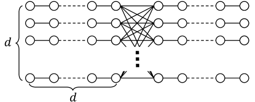
Figure 2: Example of a sparse graph that requires BFS to look at $O(d^{2})$ edges from any vertex to reach $3d$ vertices.

4.2 Heuristics for $(k,\rho)$-balls

The construction of a $(1,\rho)$-graph requires up to $n\rho$ extra edges, potentially too many to be useful for many graphs in practice. Using a small $k>1$ creates an opportunity to add fewer shortcut edges, by taking better advantange of the original edges.

To construct a $(k,\rho)$-ball, we still need to run the algorithm mentioned in Lemma 4.2, after which a shortest-path tree with $\rho$ vertices can be built. Consider the shortest-path tree $T_{s}$ starting from a source $s\in V$ that reaches out to the $\rho$ nearest vertices. Our goal is to add as few edges as possible to ensure that every $v\in T_{s}$ can be reached within $k$ hops using the combination of the original edges and the added edges $E^{\prime}$.

The following claim, which is easy to prove, shows that from the perspective of a single source vertex, the most beneficial shortcut edge goes directly from the source itself.

Claim 4.3.

An edge $(u,v)$, $u\neq s$, can be exchanged for $(s,v)$ without increasing the overall hop count from $s$.

We propose two heuristics to construct $(k,\rho)$-balls.

4.2.1 Shortcut using Greedy

To directly eliminate vertices that are more than $k$ hops away in $T_{s}$, we add edges from the root to all $(ki+1)$-hop neighbors for $i\in\mathbb{Z}^{+}$. This heuristic is simple and easy to program, but may result in adding too many edges. Consider a shortest-path tree that first forms a chain of length $k$ from the source, then the rest $\rho-k-2$ vertices all lie in the $(k+1)$-th level. The greedy heuristic will shortcut to all these $\rho-k-2$ vertices, while we can only add one edge from the source to the node in the $k$-th layer to include all vertices in $k$ hops.

4.2.2 Shortcut using Dynamic Programming (DP)

Consider, among all shortest-path trees from $s$, one where for every $v\in T_{s}$, the path $s\to v$ on $T$ has the smallest hop count possible. The optimal number of edges needed for a certain node can be computed using the following dynamic program. Let $F(u,t)$ be the number of edges into the subtree of $T_{s}$ rooted at $u$ so that every node in the subtree is at most $k$ hops away from $s$ provided that $\mbox{parent}(u)$ is at $t$ hops away from $s$. Then, for all $u\neq s$, $F(u,t)$ is given by

$$\begin{cases}1+\sum\limits_{w\in N^{+}(u)}F(w,1)&\text{ if }t=k\\ \min\mathopen{}\mathclose{{}\left(1+\sum\limits_{w\in N^{+}(u)}F(w,1),\sum\limits_{w\in N^{+}(u)}F(w,t+1)}\right)&\text{ if }t<k\\ \end{cases}$$

The number of edges needed in the end is $\sum_{u\in N^{+}(s)}F(u,0)$. The actual edges to add can be traced from the recurrence. We note that this dynamic program can be solved in $O(k\rho)$ (as $|T_{s}|=\rho$) by resolving the recurrence bottom up (using either DFS or BFS).

Note that although the dynamic programming solution gives an optimal solution for each shortest-path tree individually, the overall solution is not necessary the global optimal. Adding globally smallest number of edges to construct $(k,\rho)$-ball seems much more difficult. Yet, we show empirically in Section 5 that the dynamic programming (DP) heuristic performs very well on a wide variety of graphs—and even the greedy heuristic does well on well-structured graphs.

5 Experimental Analysis

This section empirically investigates how the settings of $k$ and $\rho$, and the choice of shortcutting heuristics affect the number of shortcut edges added, as well as the number of steps that Radius-Stepping requires. These quantities provide an indication of how well a well-engineered implementation would perform in practice.

5.1 Experiment Setup

We use graphs of various types from the SNAP datasets [17], including the road networks in Pennsylvania and Texas (real-world planer graphs) and the web graphs of the University of Notre Dame and Stanford University (real-world networks). In the case of web graphs, each edge represents a hyperlink between two web pages. We also use synthetic graphs of 2D and 3D grids (structured and unstructured grids).

In practical applications, such graphs are used both in the weighted and unweighted settings. In the weighted setting, for instance, the distances in road networks and grids can represent real distances, while the edge weights in network graphs (e.g., social networks) also have real-world meanings, such as the time required to pass a message between two users, or (the logarithm of) the probability to pass a message. In our experiments, if a graph does not come equipped with weights, we assign to every edge a random integer between $1$ and $10,000$.

We construct $(k,\rho)$-balls using the heuristics described in Section 4.2 except the implementation has the following modifications: instead of breaking ties arbitrarily and taking exactly $\rho$ neighbors, we continue until all vertices with distance $r_{\rho}(\cdot)$ are visited. This has the same implementation complexity as the theoretical description but is more deterministic. Using this, our results are a pessimistic estimate of the original heuristics as more than $\rho$ edges may be found for some sources. However, in all our experiments, we found the difference to be negligible in most instances.

To improve our confidence in the results, two of the authors have independently implemented and conducted the experiments, and arrived at the same results, even without introducing a tie-breaker.

5.2 The Number of Shortcut Edges

Section 4.2 described heuristics that put in a small number of edges to make the input graph a $(k,\rho)$-graph. How many extra edges are generated by each heuristic? To answer this question, we use 3 representative graphs in our analysis: (1) road networks in Pennsylvania, (2) a webgraph of Stanford University, and (3) a synthetic $1000$-by-$1000$ 2D grid. All these graphs have about $1$ million vertices, and between $2$ and $3$ million edges. We show experimental results for unweighted graphs since the performance of the heuristics is independent of edge weights.

Figure 3 shows the number of added edges in terms of the fraction of the original edges for $k=3$ as the value of $\rho$ is varied between $10$ and $1,000$. More detailed results are given in Tables 2 and 3 in the appendix. Evidently, both heuristics achieve similar results on the road map and 2D grid. This is because road maps and grids are relatively regular, in fact almost planar. Thus, even the naïve shortcuts to the $(ki+1)$-hop performs well. As $k$ becomes larger, the gap between the greedy and the DP heuristic increases. When $\rho$ reaches $1000$, both DP and greedy add more than $100$x edges compared to the original graph. This is because in road maps and grids the degree of a vertex is usually a small constant, which makes the shortest-path tree very deep.

On webgraphs, which is less regular, DP only adds $4$x the number of original edges even when $\rho$ is as large as $1000$ while greedy still adds $100$x the original edges. This is because webgraphs not only are far more irregular but also have a very skewed degree distribution. As a known scale-free network [1], it has some “super stars” (or more precisely, the “hubs”) in the network. In this case, the bad example in Section 4.2 occurs frequently when these hubs are not at the exact $(ki+1)$-th layer in the shortest-path tree, while the DP heuristic can discover the hubs accurately. This also explains the phenomena that only a few edges are added on webgraphs by the DP heuristic even when $\rho$ is large, since the hubs already significantly reduce the depth of the shortest path tree, and it only takes a few edges to shortcut to the hubs. This property holds for many kinds of real-world graphs such as social networks, airline networks, protein networks, and so on. In such graphs, a relatively optimal heuristic is necessary to construct the enclosed balls; a naïve method often leads to bad performance. As can be seen, the DP solution achieves satisfactory performance on webgraphs, where it only adds about 10% more edges with $k=3$ and $\rho=100$.

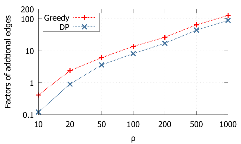
(a) Road map of Pennsylvania

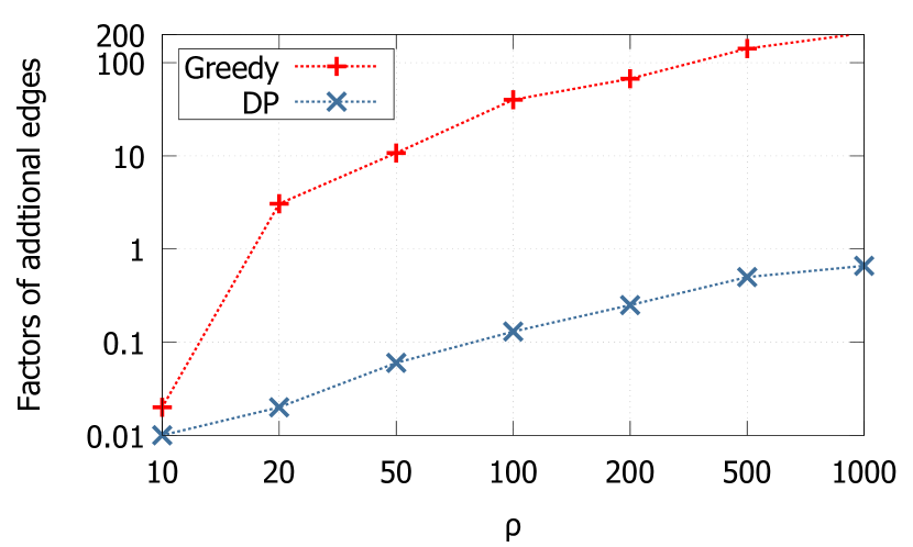
(b) Webgraph of Stanford

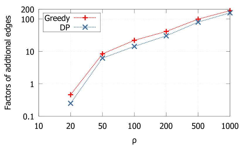
(c) 2D-grid

Figure 3: The fraction of additional edges added to generate $(k=3,\rho)$-graph using greedy vs. dynamic programming (DP) for different types of graphs.

5.3 The Number of Steps

How many steps does Radius-Stepping take for each setting of $\rho$? We ran our Radius-Stepping on both weighted and unweighted graphs and counted the number of steps as we change $\rho$. Notice that the number of steps is independent of $k$ and is only affected by $\rho$. (The value of $k$ only affects the number of substeps within a step.) We discuss the performance of our algorithm on all six graphs. Since the cost of Sssp potentially varies with the source and we cannot afford to try it from all possible sources, we take 1000 random sample sources for each graph. We use the same $1000$ sources for all our experiments for both the weighted and unweighted cases. We report the arithmetic means over all sample sources.

Unweighted Graphs (BFS): Figure 5 shows, for the unweighted case, the average number of steps taken by Radius-Stepping as $\rho$ is varied. More results appear in Tables 4 and 5 in the appendix, which compare the number of steps taken by Radius-Stepping with that of a conventional BFS implementation.

Several things are clear: on a log-log scale, the trends are downward linear as $\rho$ increases except for the Notre Dame webgraph (not completely regular but shows a similar trend). This suggests that the average number of steps is inversely proportional to $\rho$, which is consistent with our theoretical analysis.

The webgraph has a relatively smoother slope. The reason is that once the “super stars” are included in the enclosed balls, which usually only need a few hops, then most of the vertices will be visited in a few steps ($20$–$100$ steps vs. $200$–$1,500$ steps on the other graphs when $\rho=1$). However, we will later see that in the weighted case, the performances on these graphs are even better than other graphs. For the road maps and grids, the number of steps reduces steadily. Furthermore, the number of steps shown in the experiments is much less than the theoretical upper bound ($\frac{n}{\rho}\log\rho$) because most real-world graphs tend to have a hop radius that is smaller than $O(n)$.

On all the graphs studied, $\rho$ can be as small as $10$ to reduce the number of steps by $3$x. When $\rho=100$, the reduction factor is about $10$x. As the results show, we can achieve a reduction factor of more than $20$x when thousands of vertices are in the balls. The experiment results verified our theoretical analysis of the Radius-Stepping algorithm.

What should an unweighted graph look like so that Radius-Stepping reduces the steps much when adding no more than $m$ edges? At first thought, the answer might be a grid or a road map with a large diameter, so that there is more space to be reduced. However, our experiments give the opposite answer: Radius-Stepping, in fact, performs better on webgraphs with smaller diameters. On webgraphs, Radius-Stepping can reduce the number of steps by $15$x by adding no more than $m$ edges (choosing $\rho=1000$ and $k=3$), while on road maps and grids, a 5x reduction in steps requires $4m$ to $6m$ edges. Even though the number of rounds reduces more steadily and quickly on road maps and grids with larger $\rho$, the number of added edges in turn increases more rapidly (100x times more edges added to achieve 20x reduction on the number of steps). On scale-free networks, however, Radius-Stepping improves standard BFS by more than 10x in time without adding much extra edges, and an efficient implementation of Radius-Stepping on these networks might be worthwhile in the future.

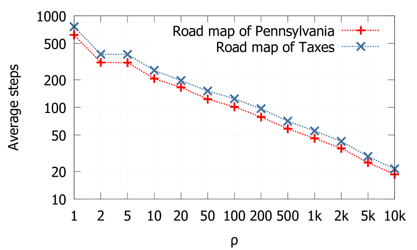
(a) Road maps

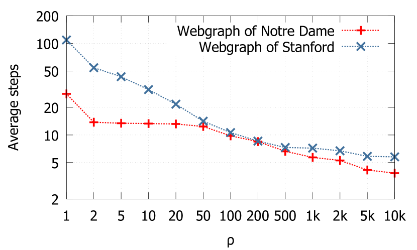
(b) Webgraphs

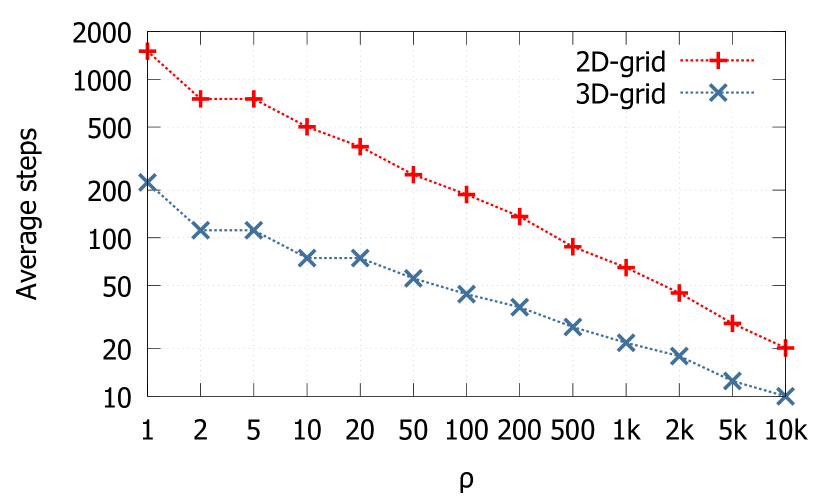
(c) Grids

Figure 4: Unweighted graphs—the number of Radius-Stepping steps as $\rho$ is varied.

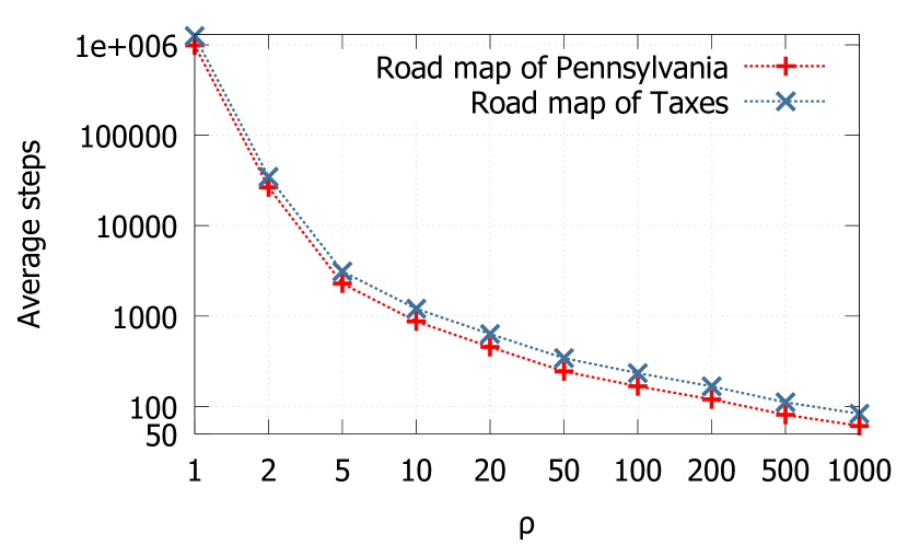
(a) Road maps

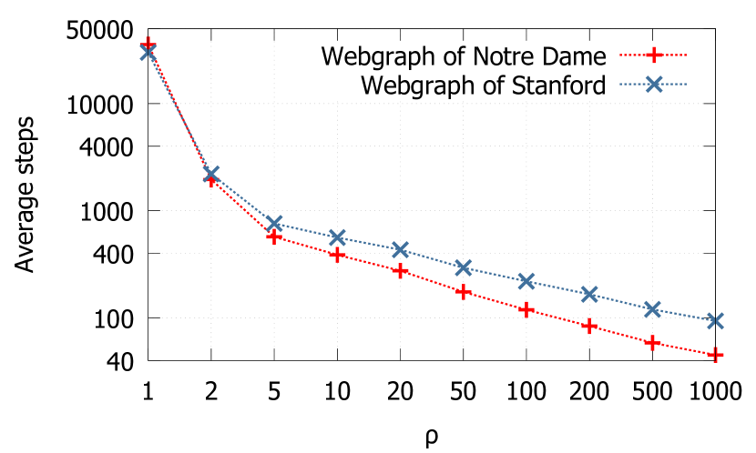
(b) Webgraphs

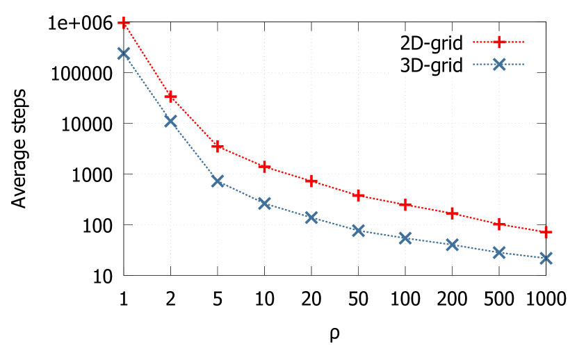
(c) Grids

Figure 5: Weighted graphs—the number of Radius-Stepping steps as $\rho$ is varied.

Weighted Graphs: Figure 5 shows, for the weighted case, the average number of steps taken by Radius-Stepping as $\rho$ is varied. More results appear in Tables 6 and 7 in the appendix, which compare the number of steps taken by Radius-Stepping to when $\rho=1$. Notice that when $\rho=1$, Radius-Stepping becomes essentially Dijkstra’s except vertices with the same distance are extracted together.

Similar to the unweighted case, the trends in Figure 5 are also nearly-linear, indicating an inverse-proportion relationship between the number of steps and $\rho$, which is consistent with our theory. In the weighted case, however, we can visit much fewer vertices in each step than those in the unweighted case because most vertices have different distances to the source. Thus, Dijkstra’s algorithm (or when $\rho=1$) requires almost $n$ steps to finish. As a result, considering the inverse-proportion relationship, even a small $\rho$ can reduce greatly the number of steps. Indeed, the number of steps taken by Radius-Stepping is far fewer than the predicted theoretical upper bound ($O(\frac{n}{\rho}\log\rho L)$ with $L=10^{4}$ here). We also notice that the number of steps decreases much faster when $\rho$ is small compared to larger values of $\rho$.

The reduction in the number of steps is significant. Even $\rho=10$ leads to about $1000$x fewer steps on road maps and grids, and about $50$–$100$x on the webgraphs. When $\rho=100$, we only need a few hundreds of steps on all graphs, which can already provide considerable parallelism. The number of steps further decreases to $20$–$80$ when $\rho=1000$. This provides some evidence that the algorithm has the potential to deliver substantial speedups when many more cores on a shared-memory machine are made available.

Another trend is that the reduction factors on the webgraphs are always less than the other two types of graphs. The reason is that the webgraphs are scale-free, and even when we do not use enclosed balls to traverse the graph, not many steps are required. The “hubs” substantially bring down the diameter of the graph. For more uniformly distributed graphs, such as the road maps and grids, increasing $\rho$ to a big value reduces the number of steps required to perform Sssp more rapidly.

5.4 How to choose the parameters?

What is the best combination of $k$ and $\rho$? The choice of $k$ and $\rho$ offers a tradeoff between the number of added edges (hence additional space and work) and the parallelism of the algorithm. In general, we do not want to increase the number of edges substantially; the total number of edges should be around $O(m)$. On every graph tested, $k=3$ or $4$ works reasonably well whereas $\rho$ in the range $50$–$100$ for weighted graph yields the best bang for the buck. A larger $\rho$ can reduce the number of steps in Radius-Stepping but in turn, increases the preprocessing time and the number of edges required to be added. A larger $k$ will reduce the number of added edges but at the same time, increases the number of visited edges, as well as the overall depth.

On unweighted graphs, Radius-Stepping performs better on webgraphs, but less efficient on grids and road maps. Finally, since preprocessing is only run once, if Sssp will be run from multiple sources, we suggest increasing $\rho$ and decreasing $k$: the cost for preprocessing is amortized over more sources.

6 Prior and Related Work

Setting	Algorithm	Work	Depth	Parameters
Unweighted (BFS)	Standard BFS	$O(m+n)$	$O(n)$
	Ullman and Yannakakis [28]	$\widetilde{O}(m\sqrt{n}+nm/t+n^{3}/t^{4})$	$\widetilde{O}(t)$	$t\leq\sqrt{n}$
	Spencer [25]	$O(m\log\rho+n\rho^{2}\log^{2}\rho)$	$O(\tfrac{n}{\rho}\log^{2}\rho)$	$\sqrt{m/n}\leq\rho\leq n$
	This work	$O(m+n\rho)$	$O(\tfrac{n}{\rho}\log\rho\log^{*}\rho)$
		preproc: $O(n\rho^{2})$	$O(\rho\log^{*}\rho)$
Weighted Sssp	Parallel Dijkstra’s [20]	$O(m+n\log n)$	$O(n\log n)$
	Parallel Dijkstra’s [4]	$O(m\log n+n)$	$O(n)$
	Klein and Subramanian [16]	$O(m\sqrt{n}\log K\log{n})$	$O(\sqrt{n}\log K\log{n})$	$K=\,$max dist. from $s$
	Spencer [25]	$O((n\rho^{2}\log\rho+m)\log(n\rho{}L))$	$O(\tfrac{n}{\rho}\log n\log(\rho{}L))$	$L=\max w(e)$, $\log({\rho{}L})\leq\rho\leq n$
	Spencer and Shi [24]	$O(\tfrac{n^{3}}{\rho^{2}}\log n\log\tfrac{n}{\rho}+m\log n)$ or $O((\tfrac{n^{3}}{\rho^{3}}+\tfrac{mn}{\rho})\log n)$	$O(\rho\log{n})$
	Cohen [6]	$O(n^{2}+n^{3}/\rho^{2})$	$O(\rho\cdot{}\mathrm{polylog}(n))$
	This work	$O((m+n\rho)\log n)$	$O(\tfrac{n}{\rho}\log n\log\rho L)$
		preproc: $O(m\log n+n\rho^{2})$ or $O(m\log n+n\rho^{2}\log\rho)$	$O(\rho^{2})$ or $O(\rho\log\rho)$

Table 1: Work/depth bounds for exact Sssp algorithms that have subcubic work.

There has been a number of research papers on the topic of parallel single-source shortest paths. In this section, we discuss prior works that are most relevant to ours (for a more comprehensive survey, see [18] and the references therein).

Some early algorithms achieve a high degree of parallism (polylogarithm depth) but with substantially more work than Dijkstra’s algorithm. Using matrix multiplications over semirings, Han et al. [12] gives an algorithm with $O(\log^{2}n)$ depth and $O(n^{3}(\log\log n/\log n)^{1/3})$ work that, in fact, solves the all-pairs shortest-path problem. With randomization, this algorithm can be implemented in $O(\log n)$ depth and $O(n^{3}\log n)$ work [11].

In another line of work, Driscoll et al. [9], refining the approach of Paige and Kruskal [20], present an $O(n\log n)$-depth algorithm with Dijkstra’s work bound. Later, Brodal et al. [4] improve the depth to $O(n)$; however, the algorithm needs $O(m\log n)$ work. We summarize in Table 1 the cost bounds for exact Sssp algorithms that have subcubic work.

By allowing a slight increase in work in exchange for a better depth bound, many algorithms have been proposed. Ullman and Yannakakis [28] describe a randomized parallel breadth-first search (BFS) that solves unweighted Sssp in $\widetilde{O}(m\sqrt{n}+nm/t+n^{3}/t^{4})$ work and $\widetilde{O}(t)$ depth for a tuneable parameter $t\leq\sqrt{n}$. The algorithm works by performing limited searches from a number of locations and adding shortcut edges with appropriate distances to speed up later traversal. Klein and Subramanian [16] extended this idea to weighted graphs, resulting in an algorithm that runs in $O(\sqrt{n}\log K\log{n})$ depth and $O(m\sqrt{n}\log K\log{n})$ work, where $K$ is the maximum weighted distance from $s$ to any node reachable from $s$. For undirected graphs, Cohen [6] presents an algorithm with $O(\rho\cdot{}\mathrm{polylog}(n))$ depth and $O(n^{2}+n^{3}/\rho^{2})$ work. Shi and Spencer [24] shows an algorithm with $O(\rho\log n)$ depth, and $O((n^{3}/\rho^{2})\log n\log(n/\rho)+m\log n)$ or $O((n^{3}/\rho^{3}+mn/\rho)\log n)$ work.

More recently, Meyers and Sanders [18] describe an algorithm called $\Delta$-stepping and analyze it for various random graph settings. Although the algorithm works well on general graphs in practice, no theoretical guarantees are known. In addition to these results, better algorithms have been developed for special classes of graphs such as planar graphs (e.g., [27, 15]) and separator-decomposable graphs [5]. There have also been approximation algorithms for Sssp. Cohen [7] describes a $(1+\varepsilon)$-algorithm for undirected graphs that runs in $O(\mathrm{polylog}(n))$ depth and $O((m+n)n^{\alpha})$ work for $\alpha>0$. Using an alternative hopset construction of Miller et al. [19], Cohen’s algorithm can be made to run in $O(m\cdot{}\mathrm{polylog}(n))$ work and $n^{1-\alpha}$ depth for $\alpha>0$.

7 Conclusion

We presented a parallel algorithm for the single-source shortest-path problem that after preprocessing, runs in $O(m\log n)$ work and $O(\tfrac{n}{\rho}\log n\log{\rho{}L})$ depth, where $\rho$ is a user-defined parameter. Compared to an optimal sequential implementation, this is only a factor of $O(\log n)$ from being work-efficient. Indeed, the algorithm offers the best-known tradeoffs between work and depth, and is conceptually simpler than prior algorithms. We leave open the question of finding a globally-optimal way to add shortcut edges for $k>1$.

Appendix A Tables for Experiments

Tables 2 to 7 show additional experimental results. Tables 2 and 3 show the number of added edges by the greedy heuristic and the dynamic programming heuristic, respectively, varying both $k$ and $\rho$. Table 4 shows the number of steps required by Radius-Stepping on different unweighted graphs with different values of $\rho$, and Table 5 shows the corresponding reduced factor compared to when $\rho=1$ (standard BFS). Table 6 shows the number of steps required by Radius-Stepping on different weighted graphs with different values of $\rho$, and Table 7 shows the corresponding reduced factor compared to when $\rho=1$ (standard Dijkstra’s).

	Roadmap of Pennsylvania					Webgraph of Stanford					2D-grid
	($|V|$=1.09M, $|E|$=3.08M)					($|V|$=281k, $|E|$=3.98M)					($|V|$=1M, $|E|$=2M)
	k				red.	k				red.	k				red.
$\bm{\rho}$	2	3	4	5	rounds	2	3	4	5	rounds	2	3	4	5	rounds
10	1.67	0.41	0.05	0.01	3.00	3.11	0.02	0.01	0.00	3.48	0.36	0.00	0.00	0.00	3.00
20	3.79	2.38	0.84	0.23	3.88	9.91	3.06	0.09	0.01	5.03	5.75	0.46	0.00	0.00	4.00
50	10.34	6.05	5.65	3.71	5.04	47.57	10.74	3.40	0.13	7.71	16.05	8.40	9.54	0.67	6.01
100	20.33	13.64	8.85	8.16	6.13	109.98	39.99	20.96	8.73	10.25	29.59	22.02	10.52	11.43	8.02
200	39.92	26.35	20.15	14.51	7.85	188.92	67.25	45.54	17.96	12.72	48.40	41.34	28.03	12.73	11.04
500	97.58	64.72	48.49	37.64	10.76	337.34	141.58	119.03	63.69	14.92	126.09	99.22	55.62	64.75	17.12
1000	192.00	127.45	95.55	75.84	13.74	529.14	208.66	219.21	149.20	15.17	243.12	181.50	129.26	108.37	23.18

Table 2: Factors of additional edges added using greedy heuristic.

	Roadmap of Pennsylvania					Webgraph of Stanford					2D-grid
	($|V|$=1.09M, $|E|$=3.08M)					($|V|$=281k, $|E|$=3.98M)					($|V|$=1M, $|E|$=2M)
	k				red.	k				red.	k				red.
$\bm{\rho}$	2	3	4	5	rounds	2	3	4	5	rounds	2	3	4	5	rounds
10	0.95	0.12	0.01	0.00	3.00	0.02	0.01	0.01	0.00	3.48	0.25	0.00	0.00	0.00	3.00
20	2.70	0.90	0.18	0.04	3.88	0.05	0.02	0.01	0.01	5.03	3.95	0.25	0.00	0.00	4.00
50	7.78	3.59	1.89	0.72	5.04	0.20	0.06	0.04	0.03	7.71	12.16	6.21	4.06	0.36	6.01
100	16.09	8.09	4.40	2.58	6.13	0.51	0.13	0.08	0.06	10.25	24.22	14.27	8.32	6.06	8.02
200	32.60	17.04	9.89	6.03	7.85	0.99	0.25	0.15	0.11	12.72	48.35	30.23	20.28	12.45	11.04
500	81.75	44.14	26.65	17.11	10.76	2.18	0.50	0.30	0.22	14.92	125.96	80.09	54.44	42.26	17.12
1000	162.91	89.30	54.82	35.95	13.74	3.92	0.66	0.34	0.24	15.17	241.30	154.97	110.87	84.87	23.18

Table 3: Factors of additional edges added using DP heuristic.

		Roadmaps		Webgraphs		Grids
		Penn	Texas	NotreDame	Stanford	2D	3D
vertices		1.09M	1.39M	325k	281k	1M	1M
edges		3.08M	3.84M	2.20M	3.98M	2M	5.94M
$\bm{\rho}$	1	619.12	761.06	28.09	108.92	1504.0	223.50
	2	309.32	380.31	13.77	54.23	751.76	111.50
	5	308.47	379.34	13.44	43.27	751.74	111.50
	10	206.30	253.71	13.32	31.29	501.14	74.50
	20	165.73	196.30	13.17	21.67	375.62	74.48
	50	123.01	151.13	12.38	14.13	250.32	55.48
	100	101.41	124.07	9.78	10.63	187.46	44.08
	200	78.61	96.92	8.47	8.56	136.24	36.48
	500	58.44	70.75	6.63	7.30	87.86	27.36
	1000	45.95	55.39	5.69	7.18	64.88	21.74
	2000	35.66	42.58	5.27	6.72	44.82	17.94
	5000	24.95	29.17	4.14	5.84	28.82	12.50
	10000	18.54	21.33	3.83	5.76	20.18	10.00

Table 4: Average number of rounds with different of $\rho$ on different unweighted graphs.

		Roadmaps		Webgraphs		Grids
		Penn	Texas	NotreDame	Stanford	2D	3D
vertices		1.09M	1.39M	325k	281k	1M	1M
edges		3.08M	3.84M	2.20M	3.98M	2M	5.94M
$\bm{\rho}$	2	2.00	2.00	2.04	2.01	2.00	2.00
	5	2.01	2.01	2.09	2.52	2.00	2.00
	10	3.00	3.00	2.11	3.48	3.00	3.00
	20	3.74	3.88	2.13	5.03	4.00	3.00
	50	5.03	5.04	2.27	7.71	6.01	4.03
	100	6.11	6.13	2.87	10.25	8.02	5.07
	200	7.88	7.85	3.32	12.72	11.04	6.13
	500	10.59	10.76	4.24	14.92	17.12	8.17
	1000	13.47	13.74	4.94	15.17	23.18	10.28
	2000	17.36	17.87	5.33	16.21	33.56	12.46
	5000	24.81	26.09	6.79	18.65	52.19	17.88
	10000	33.39	35.68	7.33	18.91	74.53	22.35

Table 5: The reduced factor of rounds on unweighted graphs comparing to BFS rounds.

		Roadmaps		Webgraphs		Grids
		Penn	Texas	NotreDame	Stanford	2D	3D
vertices		1.09M	1.39M	325k	281k	1M	1M
edges		3.08M	3.84M	2.20M	3.98M	2M	5.94M
$\bm{\rho}$	1	986K	1252K	35.6K	30.0K	965K	239K
	2	26479.9	34673.4	1953.7	2203.3	33592.2	11046.1
	5	2294.5	3123.5	571.3	759.2	3495.8	722.4
	10	872.6	1206.5	387.2	562.3	1385.0	261.9
	20	455.0	634.1	274.9	432.2	722.9	137.8
	50	245.0	343.0	174.6	293.7	375.1	76.1
	100	167.2	233.7	118.8	219.3	246.9	54.1
	200	119.8	166.9	83.7	166.0	166.9	40.2
	500	81.1	111.3	58.4	120.0	102.1	28.1
	1000	61.1	83.2	45.0	93.6	71.1	21.7

Table 6: Average number of rounds with different of $\rho$ on different weighted graphs.

		Roadmaps		Webgraphs		Grids
		Penn	Texas	NotreDame	Stanford	2D	3D
vertices		1.09M	1.39M	325k	281k	1M	1M
edges		3.08M	3.84M	2.20M	3.98M	2M	5.94M
$\bm{\rho}$	2	37.2	36.1	18.2	13.6	28.7	21.6
	5	429.7	400.8	62.3	39.6	276.1	330.6
	10	1130.0	1037.7	92.0	53.4	696.8	912.0
	20	2167.0	1974.5	129.5	69.5	1334.9	1733.3
	50	4024.5	3650.1	203.9	102.3	2572.7	3138.5
	100	5897.1	5357.3	299.7	137.0	3908.6	4414.9
	200	8230.4	7501.5	425.4	180.9	5782.0	5941.4
	500	12157.8	11248.9	609.7	250.3	9451.7	8499.8
	1000	16137.5	15048.1	791.2	320.9	13572.8	11006.6

Table 7: The reduced factor of rounds on weighted graphs comparing to $\rho=1$.

References

- [1] A.-L. Barabási and R. Albert. Emergence of scaling in random networks. science, 286(5439):509–512, 1999.
- [2] G. E. Blelloch, D. Ferizovic, and Y. Sun. Parallel ordered sets using join. arXiv preprint, 2016.
- [3] G. E. Blelloch and M. Reid-Miller. Fast set operations using treaps. In Proceedings of the tenth annual ACM symposium on Parallel algorithms and architectures, pages 16–26. ACM, 1998.
- [4] G. S. Brodal, J. L. Träff, and C. D. Zaroliagis. A parallel priority queue with constant time operations. Journal of Parallel and Distributed Computing, 49(1):4–21, 1998.
- [5] E. Cohen. Efficient parallel shortest-paths in digraphs with a separator decomposition. J. Algorithms, 21(2):331–357, 1996.
- [6] E. Cohen. Using selective path-doubling for parallel shortest-path computations. Journal of Algorithms, 22(1):30–56, 1997.
- [7] E. Cohen. Polylog-time and near-linear work approximation scheme for undirected shortest paths. Journal of the ACM (JACM), 47(1):132–166, 2000.
- [8] E. W. Dijkstra. A note on two problems in connexion with graphs. Numerische mathematik, 1(1):269–271, 1959.
- [9] J. R. Driscoll, H. N. Gabow, R. Shrairman, and R. E. Tarjan. Relaxed heaps: An alternative to fibonacci heaps with applications to parallel computation. Communications of the ACM, 31(11):1343–1354, 1988.
- [10] M. L. Fredman and R. E. Tarjan. Fibonacci heaps and their uses in improved network optimization algorithms. Journal of the ACM (JACM), 34(3):596–615, 1987.
- [11] A. M. Frieze and L. Rudolph. A parallel algorithm for all pairs shortest paths in a random graph. Management Sciences Research Group, Graduate School of Industrial Administration, Carnegie-Mellon University, 1984.
- [12] Y. Han, V. Pan, and J. Reif. Efficient parallel algorithms for computing all pair shortest paths in directed graphs. In Proceedings of the fourth annual ACM symposium on Parallel algorithms and architectures, pages 353–362. ACM, 1992.
- [13] J. Jaja. Introduction to Parallel Algorithms. Addison-Wesley Professional, 1992.
- [14] R. M. Karp and V. Ramachandran. Parallel algorithms for shared-memory machines, handbook of theoretical computer science (vol. a): algorithms and complexity, 1991.
- [15] P. N. Klein and S. Subramanian. A linear-processor polylog-time algorithm for shortest paths in planar graphs. IEEE, 1993.
- [16] P. N. Klein and S. Subramanian. A randomized parallel algorithm for single-source shortest paths. Journal of Algorithms, 25(2):205–220, 1997.
- [17] J. Leskovec and A. Krevl. SNAP Datasets:Stanford large network dataset collection. 2014.
- [18] U. Meyer and P. Sanders. -stepping: a parallelizable shortest path algorithm. J. Algorithms, 49(1), 2003.
- [19] G. L. Miller, R. Peng, A. Vladu, and S. C. Xu. Improved parallel algorithms for spanners and hopsets. In Proceedings of the 27th ACM on Symposium on Parallelism in Algorithms and Architectures, SPAA 2015, Portland, OR, USA, June 13-15, 2015, pages 192–201, 2015.
- [20] R. C. Paige and C. P. Kruskal. Parallel algorithms for shortest path problems. In ICPP’85, pages 14–20, 1985.
- [21] H. Park and K. Park. Parallel algorithms for red–black trees. Theoretical Computer Science, 262(1):415–435, 2001.
- [22] W. Paul, U. Vishkin, and H. Wagener. Parallel computation on 2-3-trees. RAIRO, Informatique théorique, 17(4):397–404, 1983.
- [23] W. J. Paul, U. Vishkin, and H. Wagener. Parallel dictionaries in 2-3 trees. In Proc. Intl. Colloq. on Automata, Languages and Programming (ICALP), pages 597–609, 1983.
- [24] H. Shi and T. H. Spencer. Time-work tradeoffs of the single-source shortest paths problem. J. Algorithms, 30(1):19–32, 1999.
- [25] T. H. Spencer. Time-work tradeoffs for parallel algorithms. Journal of the ACM (JACM), 44(5):742–778, 1997.
- [26] M. Thorup. Undirected single-source shortest paths with positive integer weights in linear time. Journal of the ACM (JACM), 46(3):362–394, 1999.
- [27] J. L. Träff and C. D. Zaroliagis. A simple parallel algorithm for the single-source shortest path problem on planar digraphs. Springer, 1996.
- [28] J. D. Ullman and M. Yannakakis. High-probability parallel transitive-closure algorithms. SIAM Journal on Computing, 20(1):100–125, 1991.