Consistent Interpretation of Molecular Simulation Kinetics Using Markov State Models Biased with External Information

Abstract

Molecular simulations can provide microscopic insight into the physical and chemical driving forces of complex molecular processes. Despite continued advancement of simulation methodology, model errors may lead to inconsistencies between simulated and reference (e.g., from experiments or higher-level simulations) observables. To bound the microscopic information generated by computer simulations within reference measurements, we propose a method that reweights the microscopic transitions of the system to improve consistency with a set of coarse kinetic observables. The method employs the well-developed Markov state modeling framework to efficiently link microscopic dynamics with long-timescale constraints, thereby consistently addressing a wide range of timescales. To emphasize the robustness of the method, we consider two distinct coarse-grained models with significant kinetic inconsistencies. When applied to the simulated conformational dynamics of small peptides, the reweighting procedure systematically improves the timescale separation of the slowest processes. Additionally, constraining the forward and backward rates between metastable states leads to slight improvement of their relative stabilities and, thus, refined equilibrium properties of the resulting model. Finally, we find that difficulties in simultaneously describing both the simulated data and the provided constraints can help identify specific limitations of the underlying simulation approach.

Despite acknowledged limitations in current all-atom (AA) force fields to describe complex molecular systems (e.g., proteinsBest, Buchete, and Hummer (2008); Cino, Choy, and Karttunen (2012)), the confidence associated with atomically-detailed molecular dynamics simulations continues to increase.Beauchamp et al. (2012) This can be attributed to improvements in simulation modelsBest and Hummer (2009); Lindorff-Larsen et al. (2010); Best et al. (2012); Jiang, Han, and Wu (2013) and methodologies,Shaw et al. (2010); Zuckerman (2011); Markwick and McCammon (2011); Fujisaki et al. (2015); Morriss-Andrews and Shea (2015) as well as continued experimental validation.Lange, van der Spoel, and de Groot (2010); Lindorff-Larsen et al. (2012) The latter has been facilitated by both increased resolution of experimentsNettels et al. (2007); Chung et al. (2012); Oikawa et al. (2013); Otosu, Ishii, and Tahara (2015) and improved toolsNoé et al. (2011); Keller, Prinz, and Noé (2012); Lindner et al. (2013); Yi et al. (2013) for comparing simulated and measured data. Beyond ongoing improvements of simulation models, the microscopic insight extracted from existing simulations can be refined by altering the trajectories to improve their agreement with external data.Groth et al. (1999); Różycki, Kim, and Hummer (2011) For example, Beauchamp et al.Beauchamp, Pande, and Das (2014) recently proposed a method to reweight the ensemble of peptide configurations generated from a molecular dynamics simulation to be consistent with experimental chemical shift and ${}^{3}J$ measurements, leading to a systematic improvement of secondary-structure propensities.

Expanding upon this idea, the present work proposes a method to improve the kinetic properties determined from a simulation, given a set of reference observables. We seek to relate the microscopic transitions of the system with much coarser observables, effectively linking a wide range of timescales. Practically, this link is provided by Markov state models (MSMs), which describe the long-time dynamics of a system with a memoryless evolution of microstate transitions. The methodology for constructing MSMs directly from simulations has been extensively developedChodera et al. (2006); Noé et al. (2009); Prinz et al. (2011a); Chodera and Noé (2014); Nüske et al. (2014); Bowman, Gregory R. and Pande, Vijay S. and Noé, Frank (2014); Wu and Noé (2015); Schütte and Sarich (2015); Vitalini, Noé, and Keller (2015) and MSMs are routinely employed to elucidate complex simulated processes, e.g., protein foldingChodera et al. (2007); Noé et al. (2007); Prinz et al. (2011b); Chodera and Pande (2011); Lane et al. (2011); Bowman, Voelz, and Pande (2011) and protein-ligand binding.Beauchamp et al. (2011); Held et al. (2011); Buch, Giorgino, and De Fabritiis (2011); Bowman and Geissler (2012); Plattner and Noé (2015) Additionally, recent workVitalini et al. (2015) has applied MSMs to identify various discrepancies in the dynamical properties generated by different AA force fields. By incorporating simulation data as well as experimental kinetic constraints, the proposed method may provide insight into the relevance and source of such discrepancies. Moreover, the approach may be particularly useful to characterize the relationship between dynamics generated by AA and coarse-grained (CG) models. This relationship is generally not well understood, limiting the applicability of a large number of CG models to static equilibrium properties.Peter and Kremer (2009); Noid (2013)

An MSM is fully characterized by a transition probability matrix, ${\bf T}(\tau)$, whose elements, $T_{ij}$, describe the probability of jumping from microstate $i$ to $j$ within a “lag time” $\tau$. The number of observed jumps between each pair of microstates during a simulation determines the count matrix, ${\bf C}^{\rm{obs}}(\tau)$. An MSM that accurately describes the long-time simulation dynamics may be constructed by maximizing the log-likelihood function $Q({\bf T})=\ln p({\bf T}\mid{\bf C}^{\rm{obs}})$, where the probability of the model given the simulation data isPrinz et al. (2011b)

$$p({\bf T}\mid{\bf C}^{\rm{obs}})\propto p({\bf C}^{\rm{obs}}\mid{\bf T})=\prod_{ij}T_{ij}^{C^{\rm{obs}}_{ij}}.$$ (1)

The proportionality follows from Bayes’ theorem, while the rightmost expression is implied by Markovian dynamics. The resulting maximum likelihood estimate (mle), ${\bf T}^{\rm mle}$, represents the MSM most likely to generate ${\bf C}^{\rm{obs}}$. Physical constraints, e.g., detailed balance, are typically incorporatedNoé (2008) into the optimization of ${\bf T}^{\rm mle}$ in order to overcome finite sampling errors of the simulation. Moreover, convex optimization routinesPrinz et al. (2011b) can efficiently determine ${\bf T}^{\rm mle}$ for MSMs with hundreds of microstates.Plattner and Noé (2015)

In the present work, we consider the mle problem (Eq. 1), while incorporating kinetic constraints, $\mathscr{F}({\bf T})=0$, between macrostates (i.e., collections of microstates). Unfortunately, these constraints are, in general, nonlinear functions of the elements $T_{ij}$, preventing the straightforward application of Lagrange multipliers or the use of convex optimization routines.Horst and Pardalos (1995) Furthermore, a simulation model may prove incompatible with $\mathscr{F}({\bf T})$, such that strict enforcement would destroy much of the microscopic information provided by the trajectory. As such, we seek to maximize the agreement with the constraints while minimally biasing the original MSM (i.e., ${\bf T}^{\rm mle}$). We achieve this balance with Metropolis Monte Carlo sampling of transition probability matrices according to

$$E_{\rm tot}({\bf T}\mid\lambda)=\lambda E_{Q}({\bf T})+(1-\lambda)E_{\mathscr{F}}({\bf T}),$$ (2)

where the energies $E_{Q}({\bf T})$ and $E_{\mathscr{F}}({\bf T})$ are shifted and rescaled quantities with respect to ${\rm Q}({\bf T})$ and $\mathscr{F}({\bf T})$, respectively.SI These quantities are defined such that $E_{Q}({\bf T}^{\rm mle})=0$, $E_{\mathscr{F}}({\bf T})=0$ when $\mathscr{F}({\bf T})=0$, and max($E_{Q}({\bf T})$), max($E_{\mathscr{F}}({\bf T})$) $\approx 1$ for the relevant range of sampled matrices. The control parameter, $\lambda$, balances the contribution of the two quantities. In practice, we monitor the two energy terms while tuning $\lambda$ in order to determine the optimal “biased” MSM. We note that when $\lambda=1$ the scheme provides the uncertainty of ${\bf T}^{\rm mle}$.Noé (2008); Metzner, Noé, and Schütte (2009); Metzner, Weber, and Schütte (2010) While we include additional technical details in the Supporting Information,SI we leave a detailed assessment to a subsequent publication. All MSM calculations employed an inhouse extension of the pyEmma package.Noé and coworkers (2015); Senne et al. (2012)

We apply the proposed method to the conformational dynamics of two small peptides. For each system, we consider simulations of both an AA and a CG model. To illustrate the robustness of the method, we consider a highly specific bottom-up model for one system while using a more transferable top-down model for the other. CG models, which lump several atoms into a single CG site, often display faster dynamics than a corresponding AA model due to reduced molecular friction between sites. As a consequence, these models are excellent candidates to test the present methodology.

For each system, we compare three distinct MSMs constructed from the simulations: (1) the “ref” model: an unbiased MSM constructed using AA data; (2) the “UMSM”: an unbiased MSM constructed using CG data; and (3) the “BMSM”: a biased MSM constructed via Monte Carlo sampling according to Eq. 2, which incorporates CG simulation data as well as external constraints. The chosen constraints involve mean first passage times (MFPTs), $\{m_{K}\}$, between metastable states determined from the ref model. The MFPTs are calculated directly from ${\bf T}$ by solving a set of linear equations.Noé and coworkers (2015); Senne et al. (2012) Here, the ref model allows a detailed assessment of the properties of the UMSM and BMSM. In general, however, a reference MSM is unnecessary, since the procedure requires only coarse (e.g., macrostate-level) information.

As expected, the CG models displayed significantly faster dynamics than the underlying AA model, allowing enhanced sampling at reduced computational expense. Ideally, a CG model should retain enhanced dynamics while consistently or predictably speeding up all relevant kinetic processes. To this end, we consider only ratios of MFPTs: $\tilde{m}_{K}\equiv m_{K}/m_{\rm L}$, where $K$ denotes a (directional) transition between two metastable states and L denotes the particular transition corresponding to the longest MFPT of the ref model. We set the constraint as the root sum square of relative errors of MFPT ratios, $\mathscr{F}=\sqrt[]{\sum_{K}\left(\tilde{m}_{K}-\tilde{m}^{\rm ref}_{K}\right)^{2}/\left(\tilde{m}^{\rm ref}_{K}\right)^{2}}$. Thus, we aim to recover the dynamics of the system up to a homogeneous speedup factor, which requires $\mathscr{F}=0$. We circumvent a calibration of the AA and CG timescales by only comparing the eigenvalues of the MSMs, $\{\lambda_{j}\}$, which are linked to the timescales of particular processes $\{j\}$ by $t_{j}=-\tau/\ln\lambda_{j}$.Bowman, Gregory R. and Pande, Vijay S. and Noé, Frank (2014) Due to the ambiguity of the CG dynamics, we report CG timescales in reduced units, $\mathcal{T}^{\rm CG}$, specific to the model.

Figure 1: Representation and relevant degrees of freedom of the CG models for (a) ${\rm Ala}_{4}$ and (b) ${\rm Ala}_{3}$. Rendered with VMD.Humphrey, Dalke, and Schulten (1996)

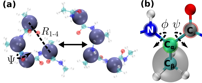
We first considered a tetra-peptide of alanine residues (${\rm Ala}_{4}$). The AA simulation employed the OPLS-AAJorgensen, Maxwell, and Tirado-Rives (1996) and SPC/EBerendsen, Grigera, and Straatsma (1987) force fields to model an explicitly solvated, capped ${\rm Ala}_{4}$ peptide. The CG simulation employed a structure-based force field,Rudzinski and Noid (2015) which represents each amino acid with a single CG site placed at the $\alpha$-carbon position, to model an implicitly solvated ${\rm Ala}_{4}$ peptide. This model qualitatively reproduces the free-energy surface (FES) along the dihedral angle, $\Psi$, defined between the four $\alpha$-carbons of the peptide backbone and the end-to-end distance, $R_{\operatorname{1-4}}$, between the first and last $\alpha$-carbons (Fig. 1a). The simulation and parameterization details were previously published.Rudzinski and Noid (2015) Both AA and CG trajectories were discretized on a uniform grid along $\Psi$ and $R_{\operatorname{1-4}}$. MSMs were constructed with lag times of $\tau=$ 250 ns and 1.25 $\mathcal{T}^{\rm S}$ for the AA and CG models, respectively, where $\mathcal{T}^{\rm S}$ denotes the time unit for the structure-based model.

Figure 2: ${\rm Ala}_{4}$. Free-energy surfaces of ${\rm Ala}_{4}$ along $\Psi$ and $R_{\operatorname{1-4}}$ determined from the (a) ref model, (c) UMSM, and (d) difference between the BMSM and UMSM. (b) Helical (H, green) and extended (E, cyan) metastable states.

Table 1: Free-energy differences (in units of $k_{\rm B}T$) with respect to the most stable metastable state for (a) ${\rm Ala}_{4}$ and (b) ${\rm Ala}_{3}$.

	(a) ${\rm Ala}_{4}$	(b) ${\rm Ala}_{3}$
	$\rm{H\operatorname{-}E}$	$\alpha\operatorname{-}\beta$	$\alpha_{\rm L}\operatorname{-}\beta$
ref	$0.51$	$0.42$	$4.18$
UMSM	$0.96$	$0.95$	$5.75$
BMSM	$0.88$	$0.75$	$5.73$

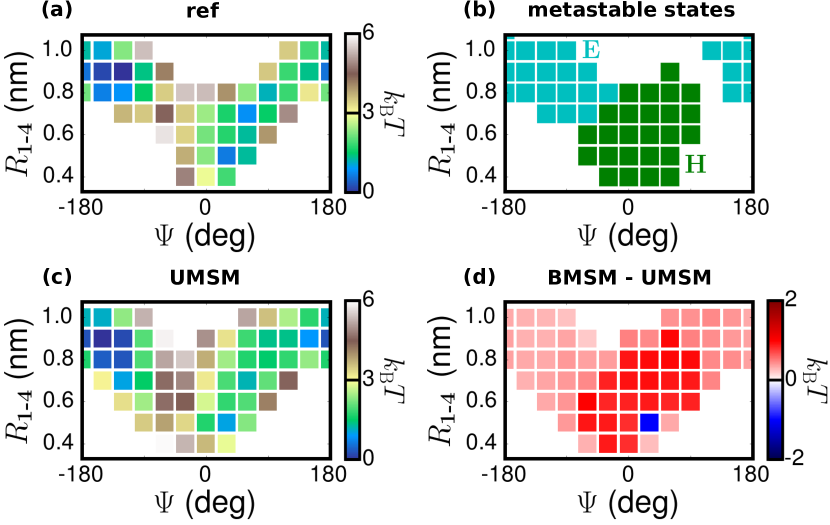
Fig. 2 compares the FESs along $\Psi$ and $R_{\operatorname{1-4}}$ determined from the ref model (panel a) and the UMSM (panel c). Additionally, panel b presents two metastable states, determined from the ref model via the PCCA+ algorithm,Deuflhard and Weber (2005) corresponding to helical (H, green) and extended (E, cyan) structures. The AA model connects these two regions through intermediates with $\Psi\approx$ 130 deg and $R_{\operatorname{1-4}}\approx$ 0.9 nm. While it is possible to describe the transition in more detail, we only consider these two states to focus on the description of the slowest process. Table 1a presents the free-energy difference between the H and E states for each model. Despite the apparent structural agreement of the FESs, the free-energy difference between the metastable states is significant.

Fig. 3 demonstrates that there are also significant discrepancies in the kinetic properties of the UMSM. We first probe the accuracy of the ratios of MFPTs between the metastable states, which will be employed as constraints in the construction of the BMSM. This agreement is assessed by calculating the relative fractional speedup, $\Gamma$, of each MFPT: $\Gamma(m_{K})\equiv\tilde{m}_{K}/\tilde{m}^{\rm ref}_{K}.$ Deviations from $\Gamma=1$ indicate discrepancies in the MFPTs, beyond a homogeneous speedup factor. The solid blue line in Fig. 3a demonstrates that the ${\rm H}\rightarrow{\rm E}$ transition is too fast compared to the reverse process in the UMSM.

The kinetic properties of the UMSM are further characterized from the eigenvalues and eigenvectors of the transition probability matrix. Fig. 3b presents the largest four eigenvalues of each model. For any MSM of a system at equilibrium, the largest eigenvalue is $\lambda_{0}=1$ and its eigenvector coincides with the equilibrium probability distribution.Bowman, Gregory R. and Pande, Vijay S. and Noé, Frank (2014) The remaining eigenvectors describe the slowest processes of the system, sorted by their eigenvalue. Fig. 3c presents the eigenvector of $\lambda_{1}$ for each model, which describes a flux of the probability distribution between microstates with positive and negative values, weighted by the individual eigenvector component of each microstate. The UMSM properly describes the transition between the two metastable states, likely due to the careful parametrization of the CG model.Rudzinski and Noid (2015) On the other hand, Fig. 3b demonstrates that the UMSM does not reproduce the implied separation of timescales between indices 1 and 2 of the ref model.

Figure 3: ${\rm Ala}_{4}$. (a) Relative fractional speedup, $\Gamma$ (defined in text), of each MFPT for the UMSM (solid lines) and BMSM (dashed lines); (b) 4 largest eigenvalues; and (c) Eigenvector characterizing the slowest dynamical process ($\lambda_{1}$) of each model. The intensity plots describe a flux of probabilities between microstates with positive and negative values, weighted by the magnitude of the individual components.

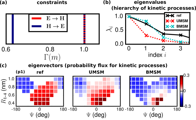
Starting with the UMSM, the constraint function, $\mathscr{F}$, built from the MFPT ratios between states ${\rm H}$ and ${\rm E}$, was applied to sample transition matrices according to Eq. 2. From the ensemble of MSMs approximately fulfilling the constraint, an optimal BMSM, sampled with $\lambda=0.875$, was chosen to balance $E_{Q}({\bf T})$ and $E_{\mathscr{F}}({\bf T})$ (see Fig. S7SI ). The blue dashed line in Fig. 3a demonstrates that the resulting BMSM nearly quantitatively reproduces the given constraint, i.e., $\Gamma(m_{\rm E\rightarrow H})\approx 1$. The BMSM yields a larger separation of timescales (Fig. 3b), in much better agreement with the ref model. However, the description of the slowest process (Fig. 3c) is somewhat degraded, with increased probability flux in a narrow region of ${\rm H}$. At the same time, the most probable microstate in this region is significantly stabilized (Fig. 2d).

The non-uniform distribution of probability flux characterizing the H to E transition is already apparent in the UMSM’s description of process 1 (Fig. 3c). Moreover, further analysis (Fig. S7 and S8SI ) indicates that this feature is not an artifact of sampling but, rather, emerges systematically from the combined application of the CG simulation and reference data to construct the BMSM. In Eq. 2, $E_{Q}$ ensures the essential dynamical features of the underlying simulation are minimally perturbed. The inclination of the BMSM to reproduce the MFPTs and timescale separation by exacerbating the concentrated probability flux of the helical region implicates this non-uniform flux as an essential component of the underlying simulated processes.

Interestingly, previous work demonstrated that the CG interaction potentials of this model stabilize helical transitions through strong, non-cooperative interactions in order to compensate for the presence of conformations sterically forbidden in the AA model.Rudzinski and Noid (2015) This feature appears to give rise to a transition from helix to extended structures that is inherently more localized within the helical state, leading to the heterogeneous flux profiles observed in the CG MSMs. Although further investigation is required to clarify the precise connection between these features, this analysis strongly implicates the methodology as a useful tool for identifying inherent limitations in the underlying simulation model.

As a second example, we also considered a tri-alanine peptide (${\rm Ala}_{3}$). The AA simulation employed the same model and implementation as described above for ${\rm Ala}_{4}$. The CG simulation employed the top-down PLUM force field,Bereau and Deserno (2009) which represents each heavy atom of the peptide backbone as well as each side chain with a CG site, to model an implicitly solvated ${\rm Ala}_{3}$ peptide. Both trajectories were discretized on a uniform grid along the $\phi$ and $\psi$ dihedral angles of the center residue (Fig. 1b). MSMs were then constructed with lag times of $\tau=$ 40 ns and 1.5 $\mathcal{T}^{\rm P}$ for the AA and CG models, respectively, where $\mathcal{T}^{\rm P}$ denotes the time unit for the PLUM model.

Figure 4: ${\rm Ala}_{3}$. Free-energy surfaces of ${\rm Ala}_{3}$ along the $\phi$ and $\psi$ dihedral angles determined from the (a) ref model, (c) UMSM, and (d) difference between the BMSM and UMSM. Panel (b) presents the definition of the three metastable states: corresponding to alpha-helical ($\alpha$, green), beta-sheet ($\beta$, blue), and left-handed-helical ($\alpha_{\rm L}$, cyan) regions.

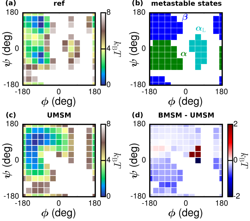
Fig. 4 compares FESs along $\phi$ and $\psi$ determined from the ref model (panel a) and the UMSM (panel c). Additionally, panel b presents three metastable states, determined from the ref model via the PCCA+ algorithm,Deuflhard and Weber (2005) corresponding to alpha-helical ($\alpha$, green), beta-sheet ($\beta$, blue), and left-handed-helical ($\alpha_{\rm L}$, cyan) structures. Panel c shows that the CG model samples the metastable states with incorrect propensities (quantified in Table 1b). In terms of kinetics, the solid lines in Fig. 5a indicate that the timescales of transition between the metastable states differ qualitatively from the ref model, beyond a homogeneous speedup factor. In this case, $\Gamma$ is determined relative to the $\alpha\rightarrow\alpha_{\rm L}$ transition. Fig. 5b demonstrates that the UMSM does not reproduce the implied separation of timescales between indices 2 and 3. Worse still, because $\lambda_{1}$ and $\lambda_{2}$ are nearly degenerate, the hierarchy of kinetic processes cannot be reliably determined. In this case, the order of these processes is qualitatively different from the ref model (Fig. 5c). While the two slowest processes of the ref model (column 1) correspond to transitions involving $\alpha_{\rm L}$ and between $\alpha$ and $\beta$, the processes of the UMSM (column 2) are in reverse order and significantly skewed.

Figure 5: ${\rm Ala}_{3}$. (a) Relative fractional speedup, $\Gamma$ (defined in text), of each MFPT for the UMSM (solid lines) and BMSM (dashed lines); (b) 4 largest eigenvalues; and (c) Eigenvectors characterizing the two slowest dynamical processes, $\lambda_{1}$ (p1) and $\lambda_{2}$ (p2) of each model. (Negative values are too small to be noticed in p1 ref and BMSM).

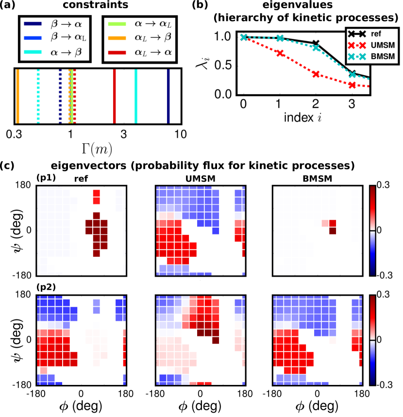
Similar to ${\rm Ala}_{4}$, the constraint $\mathscr{F}$, characterizing the error in the MFPT ratios between metastable states, was applied to sample MSMs according to Eq. 2. An optimal BMSM was identified as described above for ${\rm Ala}_{4}$, sampled with $\lambda=0.9$ (see Fig. S10SI ). In this case, the constraints could not be perfectly fulfilled without significantly deteriorating agreement with the simulation data. The dashed lines in Fig. 5a quantify this discrepancy. Fig. 4d demonstrates the BMSM’s pronounced, but localized, adjustments of microstate stabilities in the $\alpha_{\rm L}$ region, although the overall stability remains largely unchanged (Table 1b). The BMSM also slightly destabilizes the interface region between the $\alpha$ and $\beta$ metastable states, while providing an overall stabilization of both regions, resulting in a significantly improved free-energy difference (Table 1b). These adjustments result in relative fractional speedups much closer to 1 (Fig. 5a, dashed lines) as well as excellent agreement in the separation of timescales (Fig. 5b). Moreover, not only do the first two eigenvectors more accurately describe the underlying processes, but the hierarchy is also restored (Fig. 5c).

This work outlines a simple method to determine an MSM that combines information from a computer simulation with a set of kinetic constraints. Importantly, the scheme does not severely restrict the form of the constraint, allowing experimental measurements to inform the construction of the model. The proposed framework also allows simple and transparent flexibility in the enforcement of the constraints. Indeed, we find that the optimal model may not perfectly reproduce the given constraints. For the conformational dynamics of two small peptides, the BMSM improves the description of kinetics, both in terms of the constrained MFPTs and the implied timescales associated with the slowest processes, while refining slightly but systematically the equilibrium distribution of the metastable states.

In the context of CG models, the method provides a systematic framework to interpret kinetic properties in a meaningful and consistent way. We plan to investigate the transferability of micro-trajectory reweighting beyond the system used in the original calculation. Interestingly, we find that the BMSM may exacerbate artifacts of the underlying model, implicating the method as a potential tool for the refinement of molecular force fields, in the case that an underlying model is available. Finally, we expect the method will also be useful for investigations comparing high-resolution AA simulations and experimental measurements of complex biomolecular processes, e.g., protein folding.

References

- Best, Buchete, and Hummer (2008) R. B. Best, N.-V. Buchete, and G. Hummer, Biophys. J. 395, L07 (2008).
- Cino, Choy, and Karttunen (2012) E. A. Cino, W.-Y. Choy, and M. Karttunen, J. Chem. Theor. Comp. 8, 2725 (2012).
- Beauchamp et al. (2012) K. A. Beauchamp, Y.-S. Lin, R. Das, and V. S. Pande, J. Chem. Theor. Comp. 8, 1409 (2012).
- Best and Hummer (2009) R. B. Best and G. Hummer, J. Phys. Chem. B 113, 9004 (2009).
- Lindorff-Larsen et al. (2010) K. Lindorff-Larsen, S. Piana, K. Palmo, P. Maragakis, J. L. Klepeis, R. O. Dror, and D. E. Shaw, Prot. Struct. Func. Bioinfo. 78, 1950 (2010).
- Best et al. (2012) R. B. Best, X. Zhu, J. Shim, P. E. M. Lopes, J. Mittal, M. Feig, and A. D. MacKerell Jr., J. Chem. Theor. Comp. 8, 3257 (2012).
- Jiang, Han, and Wu (2013) F. Jiang, W. Han, and Y.-D. Wu, Phys. Chem. Chem. Phys. 15, 3413 (2013).
- Shaw et al. (2010) D. E. Shaw, P. Maragakis, K. Lindorff-Larsen, S. Piana, R. O. Dror, M. P. Eastwood, J. A. Bank, J. M. Jumper, J. K. Salmon, Y. B. Shan, and W. Wriggers, Science 330, 341 (2010).
- Zuckerman (2011) D. M. Zuckerman, in Annual Review of Biophysics, VOL 40, Annual Review of Biophysics, Vol. 40, edited by Rees, DC and Dill, KA and Williamson, JR (Annual Reviews, 2011) pp. 41–62.
- Markwick and McCammon (2011) P. R. L. Markwick and J. A. McCammon, Phys. Chem. Chem. Phys. 13, 20053 (2011).
- Fujisaki et al. (2015) H. Fujisaki, K. Moritsugu, Y. Matsunaga, T. Morishita, and L. Maragliano, Frontiers in bioengineering and biotechnology 3 (2015).
- Morriss-Andrews and Shea (2015) A. Morriss-Andrews and J.-E. Shea, in Annual Review of Physical Chemistry, Vol 66, Annual Review of Physical Chemistry, Vol. 66, edited by Johnson, MA and Martinez, TJ (Annual Reviews, 2015) pp. 643–666.
- Lange, van der Spoel, and de Groot (2010) O. F. Lange, D. van der Spoel, and B. L. de Groot, Biophys. J. 99, 647 (2010).
- Lindorff-Larsen et al. (2012) K. Lindorff-Larsen, P. Maragakis, S. Piana, M. P. Eastwood, R. O. Dror, and D. E. Shaw, PLoS ONE 7 (2012), 10.1371/journal.pone.0032131.
- Nettels et al. (2007) D. Nettels, I. V. Gopich, A. Hoffmann, and B. Schuler, Proc. Natl. Acad. Sci. USA 104, 2655 (2007).
- Chung et al. (2012) H. S. Chung, K. McHale, J. M. Louis, and W. A. Eaton, Science 335, 981 (2012).
- Oikawa et al. (2013) H. Oikawa, Y. Suzuki, M. Saito, K. Kamagata, M. Arai, and S. Takahashi, Scientific Reports 3 (2013), 10.1038/srep02151.
- Otosu, Ishii, and Tahara (2015) T. Otosu, K. Ishii, and T. Tahara, Nat. Commun. 6, 7685 (2015).
- Noé et al. (2011) F. Noé, S. Doose, I. Daidone, M. Löllmann, M. Sauer, J. D. Chodera, and J. C. Smith, Proc. Natl. Acad. Sci. USA 108, 4822 (2011).
- Keller, Prinz, and Noé (2012) B. G. Keller, J.-H. Prinz, and F. Noé, Chem. Phys. 396, 92 (2012).
- Lindner et al. (2013) B. Lindner, Z. Yi, J.-H. Prinz, J. C. Smith, and F. Noé, J. Chem. Phys. 139, 175101 (2013).
- Yi et al. (2013) Z. Yi, B. Lindner, J.-H. Prinz, F. Noé, and J. C. Smith, J. Chem. Phys. 139, 175102 (2013).
- Groth et al. (1999) M. Groth, J. Malicka, C. Czaplewski, S. Oldziej, L. Lankiewicz, W. Wiczk, and A. Liwo, J Biomol NMR 15, 315 (1999).
- Różycki, Kim, and Hummer (2011) B. Różycki, Y. C. Kim, and G. Hummer, Structure 19, 109 (2011).
- Beauchamp, Pande, and Das (2014) K. A. Beauchamp, V. S. Pande, and R. Das, Biophys. J. 106, 1381 (2014).
- Chodera et al. (2006) J. D. Chodera, W. C. Swope, J. W. Pitera, and K. A. Dill, Multiscale Model. Simul. 5, 1214 (2006).
- Noé et al. (2009) F. Noé, C. Schütte, E. Vanden-Eijnden, L. Reich, and T. R. Weikl, Proc. Natl. Acad. Sci. USA 106, 19011 (2009).
- Prinz et al. (2011a) J.-H. Prinz, M. Held, J. C. Smith, and Noé, Frank, Multiscale Model. Simul. 9, 545 (2011a).
- Chodera and Noé (2014) J. D. Chodera and F. Noé, Curr. Opin. Struc. Biol. 25, 135 (2014).
- Nüske et al. (2014) F. Nüske, B. Keller, G. Pérez-Hernández, M. A., and F. Noé, J. Chem. Theor. Comp. 10, 1739 (2014).
- Bowman, Gregory R. and Pande, Vijay S. and Noé, Frank (2014) Bowman, Gregory R. and Pande, Vijay S. and Noé, Frank, An Introduction to Markov State Models and Their Application to Long Timescale Molecular Simulation (Springer Science and Business Media, Dordrecht, Netherlands, 2014).
- Wu and Noé (2015) H. Wu and F. Noé, J. Chem. Phys. 142, 084104 (2015).
- Schütte and Sarich (2015) C. Schütte and M. Sarich, Eur. Phys. J. Special Topics 224, 2445 (2015).
- Vitalini, Noé, and Keller (2015) F. Vitalini, F. Noé, and B. G. Keller, J. Chem. Theor. Comp. 11, 3992 (2015).
- Chodera et al. (2007) J. D. Chodera, N. Singhal, V. S. Pande, K. A. Dill, and W. C. Swope, J. Chem. Phys. 126, 155101 (2007).
- Noé et al. (2007) F. Noé, I. Horenko, C. Schütte, and J. C. Smith, J. Chem. Phys. 126 (2007), 10.1063/1.2714539.
- Prinz et al. (2011b) J.-H. Prinz, H. Wu, M. Sarich, B. Keller, M. Senne, M. Held, J. D. Chodera, C. Schütte, and F. Noé, J. Chem. Phys. 134, 174105 (2011b).
- Chodera and Pande (2011) J. D. Chodera and V. S. Pande, Proc. Natl. Acad. Sci. USA 108, 12969 (2011).
- Lane et al. (2011) T. J. Lane, G. R. Bowman, K. Beauchamp, V. A. Voelz, and V. S. Pande, J. Am. Chem. Soc. 133, 18413 (2011).
- Bowman, Voelz, and Pande (2011) G. R. Bowman, V. A. Voelz, and V. S. Pande, J. Am. Chem. Soc. 133, 664 (2011).
- Beauchamp et al. (2011) K. A. Beauchamp, D. L. Ensign, R. Das, and V. S. Pande, Proc. Natl. Acad. Sci. USA 108, 12734 (2011).
- Held et al. (2011) M. Held, P. Metzner, J.-H. Prinz, and F. Noé, Biophys. J. 100, 701 (2011).
- Buch, Giorgino, and De Fabritiis (2011) I. Buch, T. Giorgino, and G. De Fabritiis, Proc. Natl. Acad. Sci. USA 108, 10184 (2011).
- Bowman and Geissler (2012) G. R. Bowman and P. L. Geissler, Proc. Natl. Acad. Sci. USA 109, 11681 (2012).
- Plattner and Noé (2015) N. Plattner and F. Noé, Nat. Commun. 6, 7653 (2015).
- Vitalini et al. (2015) F. Vitalini, A. S. J. S. Mey, F. Noé, and B. G. Keller, J. Chem. Phys. 142, 84101 (2015).
- Peter and Kremer (2009) C. Peter and K. Kremer, Soft Matter 5, 4357 (2009).
- Noid (2013) W. G. Noid, J. Chem. Phys. 139, 090901 (2013).
- Noé (2008) F. Noé, J. Chem. Phys. 28, 244103 (2008).
- Horst and Pardalos (1995) R. Horst and P. M. Pardalos, Handbook of Global Optimization (Springer Science and Business Media, Dordrecht, Netherlands, 1995).
- (51) See supplemental material at [URL will be inserted by AIP] for further technical details of the molecular simulations as well as Markov state model methodology and calculations.
- Metzner, Noé, and Schütte (2009) P. Metzner, F. Noé, and C. Schütte, Phys. Rev. E 80, 1 (2009).
- Metzner, Weber, and Schütte (2010) P. Metzner, M. Weber, and C. Schütte, Phys. Rev. E 82, 1 (2010).
- Noé and coworkers (2015) F. Noé and coworkers, “Pyemma,” https://github.com/markovmodel/PyEMMA/ (2015).
- Senne et al. (2012) M. Senne, B. Trendelkamp-Schroer, A. S. J. S. Mey, C. Schütte, and F. Noé, J. Chem. Theor. Comp. 8, 2223 (2012).
- Humphrey, Dalke, and Schulten (1996) W. Humphrey, A. Dalke, and K. Schulten, J. Mol. Graph. 14, 33 (1996).
- Jorgensen, Maxwell, and Tirado-Rives (1996) W. L. Jorgensen, D. S. Maxwell, and J. Tirado-Rives, J. Am. Chem. Soc. 118, 11225 (1996).
- Berendsen, Grigera, and Straatsma (1987) H. Berendsen, J. Grigera, and T. Straatsma, J. Phys. Chem. 91, 6269 (1987).
- Rudzinski and Noid (2015) J. F. Rudzinski and W. G. Noid, J. Chem. Theor. Comp. 11, 1278 (2015).
- Deuflhard and Weber (2005) P. Deuflhard and M. Weber, Linear Algebra Appl 398, 161 (2005).
- Bereau and Deserno (2009) T. Bereau and M. Deserno, J. Chem. Phys. 130, 235106 (2009).