Basin stability approach for quantifying responses of multistable systems with parameters mismatch

Abstract

In this paper we propose a new method to detect and classify coexisting solutions in nonlinear systems. We focus on mechanical and structural systems where we usually avoid multistability for safety and reliability. We want to be sure that in the given range of parameters and initial conditions the expected solution is the only possible or at least has dominant basin of attraction. We propose an algorithm to estimate the probability of reaching the solution in given (accessible) ranges of initial conditions and parameters. We use a modified method of basin stability (Menck et. al., Nature Physics, 9(2) 2013). In our investigation we examine three different systems: a Duffing oscillator with a tuned mass absorber, a bilinear impacting oscillator and a beam with attached rotating pendula. We present the results that prove the usefulness of the proposed algorithm and highlight its strengths in comparison with classical analysis of nonlinear systems (analytical solutions, path-following, basin of attraction ect.). We show that with relatively small computational effort (comparing to classical analysis) we can predict the behaviour of the system and select the ranges in parameter’s space where the system behaves in a presumed way. The method can be used in all types of nonlinear complex systems.

1 Introduction

In mechanical and structural systems the knowledge of all possible solutions is crucial for safety and reliability. In devices modelled by linear ordinary differential equations we can predict the existing solutions using analytical methods [29, 25]. However, in case of complex, nonlinear systems analytical methods do not give the full view of system’s dynamics [31, 20, 3, 24]. Due to nonlinearity, for the same set of parameters more then one stable solution may exist [16, 11, 32, 18, 7, 23, 22]. This phenomenon is called multistability and has been widely investigated in all types of dynamical systems (mechanical, electrical, biological, neurobiological, climate and many more). The number of coexisting solutions strongly depends on the type of nonlinearity, the number of degrees of freedom and the type of coupling between the subsystems. Hence, usually the number of solutions vary strongly when values of system’s parameters changes.

As an example, we point out the classical tuned mass absorber [2, 9, 1, 17, 30, 21, 12, 6]. This device is well known and widely used to absorb energy and mitigate unwanted vibrations. However, the best damping ability is achieved in the neighbourhood of the multistability zone [7]. Among all coexisting solutions only one mitigates oscillations effectively. Other solutions may even amplify an amplitude of the base system. So, it is clear that only by analyzing all possible solutions we can make the device robust.

Similarly, in systems with impacts one solution can ensure correct operation of a machine, while others may lead to damage or destruction [5, 4, 14, 28, 15]. The same phenomena is present in multi-degree of freedom systems where interactions between modes and internal resonances play an important role [8, 19, 10, 26].

Practically, in nonlinear dynamical systems with more then one degree of freedom it is impossible to find all existing solutions without huge effort and using classical methods of analytical and numerical investigation (path-following, numerical integration, basins of attractions), especially in cases when we analyse a wider range of system’s parameters and we cannot precisely predict the initial conditions. Moreover, solutions obtained by integration may have meager basins of attraction and it could be hard or even impossible to achieve them in reality. That is why we propose here a new method basing on the idea of basin stability [23]. The classical basin stability method is based on the idea of Bernoulli trials, i.e., equations of system’s motion are integrated $N$ times for randomly chosen initial conditions (in each trial they are different). Analyzing the results we asses the stability of each solution. If there exist only one solution the result of all trials is the same. But, if more attractors coexist we can estimate the probability of their occurrence for a chosen set of initial conditions. In mechanical and structural systems we want to be sure that a presumed solution is stable and has the dominant basin of attraction in a given range of system’s parameters. Therefore, we build up a basin stability method by drawing values of system’s parameters. We take into account the fact that values of parameters are measured or estimated with some finite precision and also that they can slightly vary during normal operation.

The paper is organized as follows. In Section 2 we introduce simple models which we use to demonstrate the main idea of our approach. In the next section we present and describe the proposed method. Section 4 includes numerical examples for systems described in Section 2. Finally, in Section 5 our conclusions are given.

2 Model of systems

In this section we present systems that we use to present our method. Two models are taken from our previous papers [7, 13] and the third one was described by Pavlovskaia et. al. [27]. We deliberately picked models whose dynamics is well described because we can easily evaluate the correctness and efficiency of the method we propose.

2.1 Tuned mass absorber coupled to a Duffing oscillator

The first example is a system with a Duffing oscillator and a tuned mass absorber. It was investigated in [7] and is shown in Figure 1. The main body consists of mass $M$ fixed to the ground with nonlinear spring (hardening characteristic $k_{1}+k_{2}y^{2}$) and a viscous damper (damping coefficient $c_{1}$). The main mass is forced externally by a harmonic excitation with amplitude $F$ and frequency $\omega$. The absorber is modelled as a mathematical pendulum with length $l$ and mass $m$. A small viscous damping is present in the pivot of the pendulum.

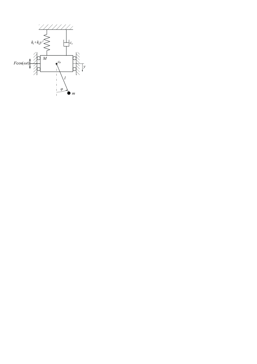
Figure 1: The model of the first considered system. Externally forced Duffing oscillator with attached pendulum (tuned mass absorber).

The equations of the system’s motion are derived in [7], hence we do not present their dimension form. Based on the following transformation of coordinates and parameters we reach the dimensionless form: $\omega_{1}^{2}=\frac{k_{1}}{M+m}$, $\omega_{2}^{2}=\frac{g}{l}$, $a=\frac{m}{M+m}$, $b=\left(\frac{\omega_{2}}{\omega_{1}}\right)^{2}$, $\alpha=\frac{k_{2}l^{2}}{(M+m)\omega_{1}^{2}}$, $f=\frac{F}{(M+m)l\omega_{1}^{2}},$ $d_{1}=\frac{c_{x}}{(M+m)\omega_{1}}$, $d_{2}=\frac{c_{\varphi}}{ml^{2}\omega_{2}}$, $\mu=\frac{\omega}{\omega_{1}}$, $\tau=t\omega_{1}$, $x=\frac{y}{l}$, $\dot{x}=\frac{\dot{y}}{\omega_{1}l}$, $\ddot{x}=\frac{\ddot{y}}{\omega_{1}^{2}l}$, $\gamma=\varphi,$ $\dot{\gamma}=\frac{\dot{\varphi}}{\omega_{2}},$ $\gamma=\frac{\ddot{\varphi}}{\omega_{2}^{2}}$.

The dimensionless equations are as follows:

$$\begin{array}[]{c}\ddot{x}-ab\ddot{\gamma}\sin\gamma-ab\dot{\gamma}^{2}\cos\gamma+x+\alpha x^{3}+d_{1}\dot{x}=f\cos\mu\tau,\\ \\ \ddot{\gamma}-\frac{1}{b}\ddot{x}\sin\gamma+\sin\gamma+d_{2}\dot{\gamma}=0,\end{array}$$ (1)

where $\mu$ is the frequency of the external forcing and we consider it as controlling parameter. The dimensionless parameters have the following values: $f=0.5$, $a=0.091$, $b=3.33$, $\alpha=0.031$, $d_{1}=0.132$ and $d_{2}=0.02$. Both subsystems (Duffing oscillator and the pendulum) have a linear resonance for $\mu=1.0$.

2.2 System with impacts

As the next example we analyse a system with impacts [27]. It is shown in Figure 2 and consists of mass $M$ suspended by a linear spring with stiffness $k_{1}$ and a viscous damper with the damping coefficient $c$ to harmonically moving frame. The frame oscillates with amplitude $A$ and frequency $\Omega$. When amplitude of mass $M$ motion reaches the value $g$, we observe soft impacts (spring $k_{2}$ is much stiffer than spring $k_{1}$).

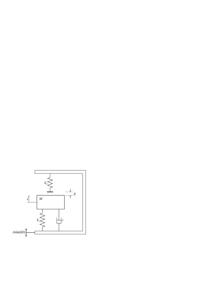
Figure 2: The model of the second considered system. Externally forced oscillator with impacts.

The dimensionless equation of motion is as follow (for derivation see [27]) :

$$\ddot{x}+2\xi\dot{x}+x+\beta\left(x-e\right)\mathrm{H}\left(x-e\right)=a\omega^{2}\sin\left(\omega\tau\right)$$

where $x=\frac{y}{y_{0}}$ is the dimensionless vertical displacement of mass $M$, $\tau=\omega_{n}t$ is the dimensionless time, $\omega_{n}=\frac{k_{1}}{M}$, $\beta=\frac{k_{2}}{k_{1}}$ the stiffness ratio, $e=\frac{g}{y_{0}}$ the dimensionless gap between equilibrium of mass $M$ and the stop suspended on the spring $k_{2}$, $a=\frac{A}{y_{0}}$ and $\omega=\frac{\Omega}{\omega_{n}}$ are dimensionless amplitude and frequency of excitation, $\xi=\frac{c}{2m\omega_{n}}$ is the damping ratio, $y_{0}=1.0\>[\mathrm{mm}]$ and $\mathrm{H}(\cdot)$ the Heaviside function. In our calculations we take the following values of system’s parameters: $a=0.7$, $\xi=0.01$, $\beta=29$, $e=1.26$. As a controlling parameter we use the frequency of excitation $\omega$.

2.3 Beam with suspended rotating pendula

The last considered system consists of a beam which can move in the horizontal direction and $n$ rotating pendula. The beam has the mass $M$ and supports $n$ rotating, excited pendula. Each pendulum has the same length $l$ and masses $m_{i}$ $(i=1,\>2,\ldots,\>n)$. We show the system in Figure 3 [13]. The rotation of the $i$-th pendulum is given by the variable $\varphi_{i}$ and its motion is damped by the viscous friction described by the damping coefficient $c_{\varphi}$. The forces of inertia of each pendulum acts on the beam causing its motion in the horizontal direction (described by the coordinate $x$). The beam is considered as a rigid body, so we do not consider the elastic waves along it. We describe the phenomena which take place far below the resonances for longitudinal oscillations of the beam. The beam is connected to a stationary base by a light spring with the stiffness coefficient $k_{x}$ and viscous damper with a damping coefficient $c_{x}$. The pendula are excited by external torques proportional to their velocities: $N_{0}-\dot{\varphi}_{i}N_{1}$, where $N_{0}$ and $N_{1}$ are constants. If no other external forces act on the pendulum, it rotates with the constant velocity $\omega=N_{0}/N_{1}$. If the system is in a gravitational field (where $g=9.81\>[\mathrm{m/s^{2}}]$ is the acceleration due to gravity), the weight of the pendulum causes the unevenness of its rotation velocity, i.e., the pendulum slows down when the centre of its mass goes up and accelerates when the centre of its mass goes down.

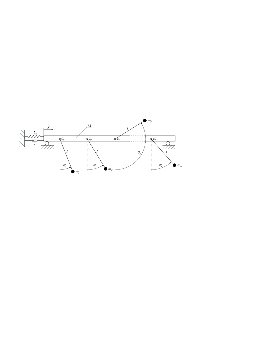
Figure 3: The model of the third considered system. Horizontally moving beam with attached pendulums.

The system is described by the following set of dimensionless equations:

$$m_{i}l^{2}\ddot{\varphi}_{i}+m_{i}\ddot{x}l\cos{\varphi_{i}}+c_{\varphi}\dot{\varphi}_{i}+m_{i}gl\sin{\varphi_{i}}=N_{0}-\dot{\varphi}_{i}N_{1}$$ (2)

$$\left({M+\sum\limits_{i=1}^{n}{m_{i}}}\right)\ddot{x}+c_{x}\dot{x}+k_{x}x=\sum\limits_{i=1}^{n}{m_{i}l\left({-\ddot{\varphi}_{i}\cos\varphi_{i}+\dot{\varphi}_{i}^{2}\sin\varphi_{i}}\right)}$$ (3)

In our investigation we analyze two cases: a system with two pendula (where $n=2$ and $i=1,\>2$) and with $20$ pendula ($n=20$ $i=1,\>2,\>...,n$).. The values of the parameters are as follows: $m_{i}=\frac{2.00}{n}$, $l=0.25$, $c_{\varphi}=\frac{0.02}{n}$, $N_{0}=5.0$0, $N_{1}=0.50$, $M=6.00$, $g=9.81$, $c_{x}=\frac{\ln\left(1.5\right)}{\pi}\sqrt{k_{x}\left(M+\sum\limits_{i=1}^{n}{m_{i}}\right)}$and $k_{x}$ is a controlling parameter. The derivation of the system’s equations can be found in [13]. We present the transformation to a dimensionless form in Appendix A.

3 Methodology

In [23] Authors present a “basin stability” method which let us estimate the stability and number of solutions for given values of system parameters. The idea behind basin stability is simple, but it is a powerful tool to assess the size of complex basins of attraction in multidimensional systems. For fixed values of system’s parameters, $N$ sets of random initial conditions are taken. For each set we check the type of final attractor. Based on this we calculate the chance to reach a given solution and determine the distribution of the probability for all coexisting solutions. This gives us information about the number of stable solutions and the sizes of their basins of attraction.

We consider the dynamical system $\dot{\mathbf{x}}=f\,(\mathbf{x},\,\omega)$, where $\mathbf{x}\in\mathtt{\mathbb{R}^{n}}$ and $\omega\in\mathbb{R}$ is the system’s parameter. Let ${\cal B\subset\mathbb{\mathtt{\mathbb{R}^{n}}}}$ be a set of all possible initial conditions and ${\cal C}\subset\mathbb{\mathtt{\mathbb{R}}}$ a set of accessible values of system’s parameter. Let us assume that an attractor ${\cal A}$ exists for $\omega\in{\cal C_{A}}\subset{\cal C}$ and has a basin of attraction $\beta({\cal A})$. Assuming random initial conditions the probability that the system will reach attractor ${\cal A}$ is given by $p\left({\cal A}\right)$. If this probability is equal to $p\left({\cal A}\right)=1.0$ this means that the considered solution is the only one in the taken range of initial conditions and given values of parameters. Otherwise other attractors coexist. The initial conditions of the system are random from set ${\cal B_{A}}\subset{\cal B}$. We can consider two possible ways to select this set.

I

The first ensures that set the ${\cal B_{A}}$ includes values of initial conditions leading to all possible solutions. This approach is appropriate if we want to get a general overview of the system’s dynamics.

II

In the second approach we use a narrowed set of initial conditions that corresponds to practically accessible initial states.…

In our method we chose the second approach because it let us take into account constrains imposed on the system and because in engineering we usually know or expect the initial state of the system with some finite precision.

In the classical approach of Menck et. al. [23] the values of system’s parameters are fixed and do not change during calculations. The novelty of our method is that we not only draw initial conditions but also values of some selected parameters of the system. We assume that the initial conditions and some of the system’s parameters are chosen randomly. Then using $N$ trials of numerical simulations we estimate the probability that the system will reach a given attractor ${\cal A}$ ($p\left({\cal A}\right)$). The idea is to take into consideration the fact that the values of system’s parameters are measured or estimated with some finite accuracy which is often hard to determine. Moreover values of parameters can vary during normal operation. Therefore drawing valus of parameters we can describe how a mismatch in their values influences the dynamics of the system and estimate the risk of failure. In many practical applications one is interested in reaching only one presumed solution ${\cal A}$, and the precise description of other coexisting attractors is not necessary. We usually want to know the probability of reaching the expected solution $p\left({\cal A}\right)$ and the chance that the system behave differently. If $p\left({\cal A}\right)$ is sufficiently large, we can treat the other attractors as an element of failure risk.

In our approach we perform the following steps:

I

We pick values of system’s parameters from the set ${\cal C_{A}}\subset{\cal C}$.

II

We select the set ${\cal C_{A}}$ so that it consists of all practically accessible values of system’s parameters $\omega$ . This let us ensure that a given solution indeed exists in a practically accessible range (taking into account the mismatch in parameters).

III

We subdivide the set $C_{A}$ in to $m=1,2,\dots M$ equally spaced subsets. The subsets ${\cal C}_{A}^{m}$ do not overlap and the relation $\bigcup_{m=1\dots M}{\cal C}_{A}^{m}=C_{A}$ is always fulfilled.

IV

Then for each subset ${\cal C}_{A}^{m}$ we randomly pick $N$ sets of initial conditions and value of the considered parameter. For each set we check the final attractor of the system.

V

After a suficient number of trials we calculate the probability of reaching a presumed solution or solutions.

VI

Finally we describe the relation between the value of the system’s parameter and the “basin stability” of reachable solutions.…

In our calculations for each range of parameter values (subset ${\cal C}_{A}^{m}$) we draw from $N=100$ up to $N=1000$ sets of initial conditions and parameter. The value of $N$ strongly depends on the complexity of the analysed system. Also the computation time for a single trial should be adjusted for each system independently such that it can reach the final attractor. In general, we recommend that in most cases $N$ should be at least 100.

4 Numerical results

4.1 Tuned mass absorber coupled to a Duffing oscillator

At the beginning we want to recall the results we present in our previous paper [7]. As a a summary we show Figure 4 with a two dimensional bifurcation diagram obtained by the path-following method. It gives bifurcations for varying amplitude $f$ and frequency $\mu$ of the external excitation (see Eq. 1). Lines shown in the plot correspond to different types of bifurcations (period doubling, symmetry breaking, Neimark-Sacker and resonance tongues). We present these lines in one style because the structure is too complex to follow bifurcation scenarios and we do not need that data (details are shown in [7]). We mark areas where we observe the existence of one solution (black colour), or the coexistence of two (grey) and three (hatched area) stable solutions. The remaining part of the diagram (white area) corresponds to situations where there are four or more solutions. Additionally, by white colour we also mark areas where only the Duffing system is oscillating in 1:1 resonance with the frequency of excitation and the pendulum is in a stable equilibrium position, i.e., HDP (hanging down pendulum) state. In this case the dynamics of the system is reduced to the oscillations of summary mass ($M+m$).

The detailed analysis of system 1 is time consuming and creation of Figure 4 was preceded by complex analysis done with large computational effort. Additionally, the obtained results give us no information about the size of the basins of attraction of each solution - which practically means that some of the solutions may occur only very rarely in the real system (i.e. due to not accessible initial conditions). Nevertheless, such analysis gives us an in-depth knowledge about the bifurcation structure of the system. As we can see, the range where less then three solutions exist is rather small, especially for $\mu<2.0$. To illustrate our method of analysis, we focus on three solutions: $2:1$ oscillating resonance, HDP and $1:1$ rotating resonance assuming that only they have some practical meaning.

Figure 4: Two-parameter bifurcations diagram of the system (1) in the plane $\left(f,\,\mu\right)$ showing periodic oscillations and rotations of the pendulum. Black colour indicates one attractor, grey colour shows two coexisting attractors (the same as for black but with a coexisting stable steady state of the pendulum). In the hatched area we observe the coexistence of stable rotations and a stable steady state of the pendulum. A detailed analysis is presented in [7].

To show our results obtained with integration, we compute bifurcation diagrams for $f=0.5$ in the range $\mu\in[0.1,\>3.0]$ (see Figure 5). In Figure 5(a) we increase $\mu$ from $0.1$ to $3.0$ and in Figure 5(b) we decrease $\mu$ from $3.0$ to $0.1$. As the initial conditions we take the equilibrium position ($x_{0}=\dot{x}_{0}=0.0$ and $\gamma_{0}=\dot{\gamma}_{0}=0.0$). In both panels we plot the amplitude of the pendulum $\gamma$. Ranges where the diagrams differ we mark by grey rectangles. It is easy to see that there are two dominating solutions: HDP and $2:1$ internal resonance. Near $\mu=1.0$ we observe a narrow range of $1:1$ and $9:9$ resonances and chaotic motion (for details see Figure 6 in [7]). Based on previous results we know that we detected all solutions existing in the considered range, however we do not have information about the size of their basins of attraction and coexistence. Hence the analysis with the proposed method should give us new important information about the system’s dynamics. Contrary to the bifurcation diagram obtained by path-following in Figure 5, we do not observe rotating solutions (the other set of initial conditions should be taken).

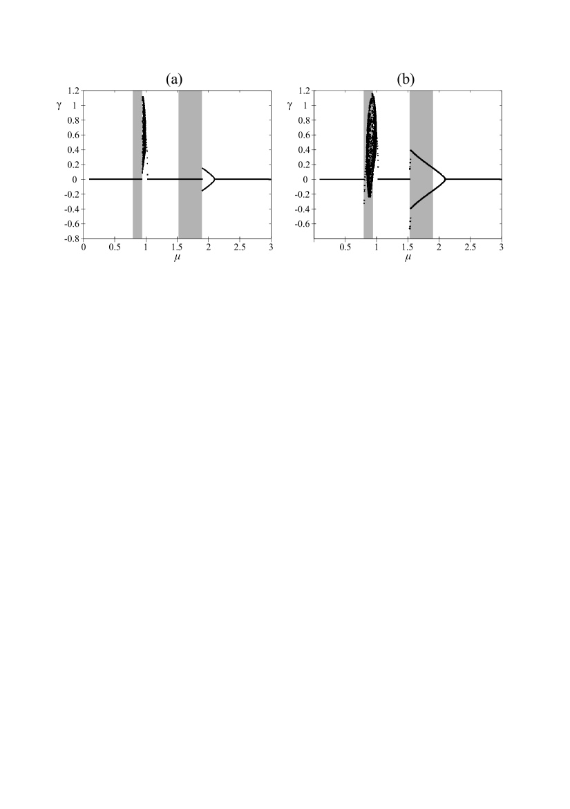
Figure 5: Bifurcation diagram showing the behaviour of the pendulum suspended on the Duffing oscillator. For subplot (a) the value of the bifurcation parameter $\mu$ was increased, while for subplot (b) we decreased the value of $\mu$. Gray rectangles mark the range of the bifurcation parameter $\mu$ for which different attractors coexist. A detailed analysis is presented in [7].

In Figure 6 we show the probability of reaching the three aforementioned solutions obtained using the proposed method. The initial conditions are random numbers drawn from the following ranges: $x_{0}\in[-2,\>2]$, $\dot{x}_{0}\in[-2,\>2]$, $\gamma_{0}\in[-\pi,\>\pi]$ and $\dot{\gamma}_{0}\in[-2.0,\>2.0]$ (ranges there selected basing on the results from [7]). The frequency of excitation is within a range $\mu\in[0,\>3.0]$ (Figure 6(a,c) ), then we refine it to $\mu\in[1.25,\>2.75]$ (Figure 6(b,d) ). In both cases we take $15$ equally spaced subsets of $\mu$ and in each subset we calculate the probability of reaching a given solution. For each subset we calculate $100$ trials each time drawing initial conditions of the system and a value of $\mu$ from the appropriate range. Then we plot the dot in the middle of the subset which indicate the probability of reaching a given solution in each considered range. Lines that connect the dots are shown just to ephasize the tendency. For each range we take $N=1000$ because we want to estimate the probability of a solution with small a basin of stability (1:1 rotating periodic solution).

As we can see in Figure 4, the $2:1$ resonance solution exists in the area marked by black colour around $\mu=2.0$ and coexists with HDP in the neighbouring grey zone. In Figure 6 we mark the probability of reaching the $2:1$ resonance using blue dots. As we expected, for $\mu<1.4$ and $\mu>2.2$ the solution does not exist. In the range $\mu\in[1.4,\>2.2]$ the maximum value of probability $p(2:1)=0.971$ is reached in the subset $\mu\in[1.8,\>2.0]$ and outside that range the probability decreases. To check if we can reach $p(2:1)=1.0$, we decrease the range of parameter’s values to $\mu\in[1.25,\>2.75]$ and the size of subset to $\Delta\mu=0.1$ (we still have 15 equally spaced subsets). The results are shown in Figure 6(b) similarly in blue colour. In the range $\mu\in[1.95,\>2.05]$ the probability $p(2:1)$ is equal to unity and in the range $\mu\in[1.85,\>1.95]$ it is slightly smaller $p(2:1)=0.992$. Hence, for both subsets we can be nearly sure that the system reaches the $2:1$ solution. This gives us indication of how precise we have to set the value of $\mu$ to be sure that the system will behave in a presumed way.

A similar analysis is performed for HDP. The values of probability is indicated by the red dots. As one can see for $\mu<0.8$, $\mu\in[1.2,\>1.4]$ and $\mu\in[2.6,\>2.8]$, the HDP is the only existing solution. The rapid decrease close to $\mu\approx 1.0$ indicates the $1:1$ resonance and the presence of other coexisting solutions in this range (see [7]). In the range $\mu\in[1.2,\>1.4]$ the probability $p(\mathrm{HDP})=1.0$ which corresponds to a border between solutions born from $1:1$ and $2:1$ resonance. Hence, up to $\mu=2.0$ the probability of the HDP solution is a mirror refection of $p(2:1)$. The same tendency is observed in the narrowed range as presented in Figure 6(b). Finally, for $\mu>2.0$ the third considered solution comes in and we start to observe an increase of probability of the rotating solution $S(\mu,\>\mathrm{HDP})$ as shown in Figure 6(c). However, the chance of reaching the rotating solution remains small and never exceeds $p(\mathrm{1:1})=8\times 10^{-3}$. We also plot the probability of reaching the rotating solution in the narrower range of $\mu$ in Figure 6(d). The probability is similar to the one presented in Figure 6(c) - it is low and does not exceed $p(\mathrm{1:1})=8\times 10^{-3}$. Note that the results presented in Figure 6(a,b) and Figure 6(c,d) are computed for different sets of random initial conditions and parameter values; hence the obtained probability can be slightly different.

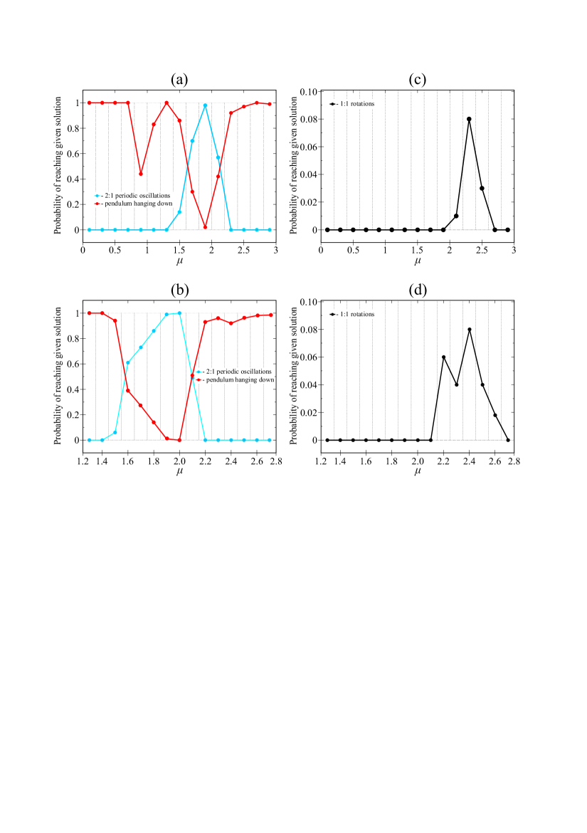
Figure 6: Probability of reaching given solutions in (1) system with tuned mass absorber. Subplots (a,b) present solutions with $2:1$ periodic oscillations (blue) and without motion of the pendulum (red). Subplots (c,d) present the probability of reaching $1:1$ rotations (black). (Please note that in both cases (a,b) and (c,d) the initial conditions and parameter are somehow random, hence the results may slightly differ).

4.2 System with impacts

In this subsection we present our analysis of different periodic solutions in the system with impacts. A discontinuity usually increases the number of coexisting solutions. Hence, in the considered system we observe a large number of different stable orbits and their classification is necessary. In Figure 7 we show two bifurcation diagrams with $\omega$ as controlling parameter. Both of them start with initial conditions $x_{0}=0.0$ and $\dot{x}_{0}=0.0$. In panel (a) we increase $\omega$ from $0.801$ to $0.8075$; while in panel (b) we decrease $\omega$ in the same range. We select the range of $\omega$ basing on the results presented in [27]. As one can see, both diagrams differ in two zones marked by grey colour. Hence, we observe a coexistence of different solutions, i.e., in the range $\omega\in[0.8033,\>0.8044]$ solutions with period-3 and -2 are present, while in the range $\omega\in[0.8068,\>0.8075]$ we detected solutions with period-2 and -5. As presented in [27] some solutions appear from a saddle-node bifurcation and we are not able to detect them with the classical bifurcation diagram. The proposed method solves this problem and shows all existing solutions in the considered range of excitation frequency.

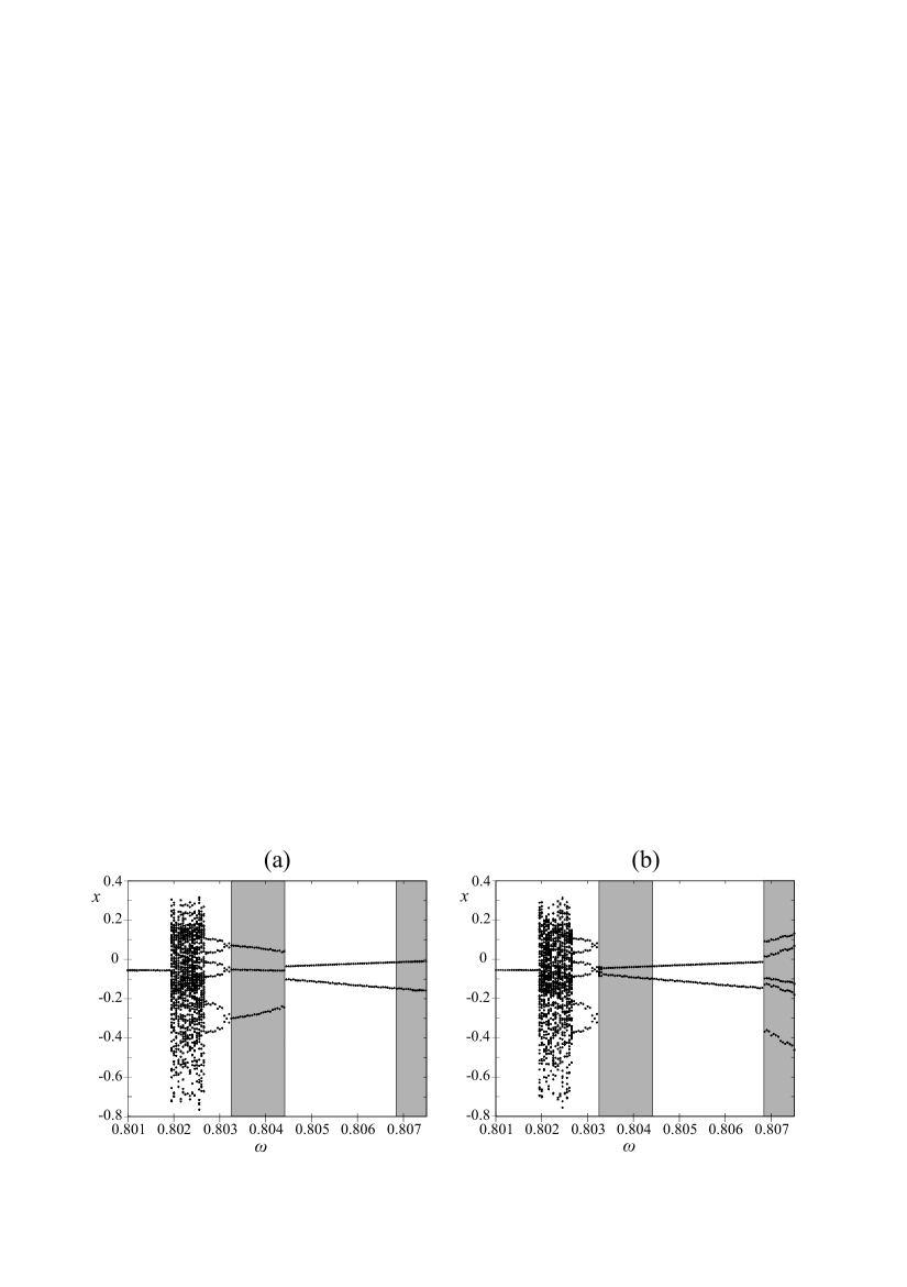
Figure 7: Bifurcation diagram showing the behaviour of impacting oscillator (2). For subplot (a) the value of the bifurcation parameter $\omega$ was increased while for subplot (b) we decreased the value of $\omega$. Grey rectangles mark the range of the bifurcation parameter $\omega$ for which different attractors coexist. Further analysis can be found in [27].

We focus on periodic solutions with periods that are not longer than eight periods of excitation. We observe periodic solutions with higher periods in the narrow range of $\omega$ but the probability that they will occur is very small and we can neglect them. All non-periodic solutions are chaotic (quasiperiodic solutions are not present in this system). The results of our calculations are shown in Figure 8(a,b). We take initial conditions from the following ranges $x_{0}\in[-2,\>2]$, $\dot{x}_{0}\in[-2,\>2]$. The controlling parameter $\omega$ is changed from $0.801$ to $0.8075$ with step $\Delta\omega=0.0005$ in Figure 8(a) and from $0.806$ to $0.8075$ with the step $\Delta\omega=0.0001$ in Figure 8(b) (in each subrange of excitation’s frequency we pick the exact value of $\omega$ randomly from this subset). The probability of periodic solutions is plotted by lines with different colours and markers. We detect the following solutions: period-1, -2, -3, -5 (two different attractors with large and small amplitude), -6 and -8. The dot lines indicate the sum of all periodic solutions’ probability (also with period higher then eight). Hence, when its value is below $1$, chaotic solution exist. Dots are drawn for mean value i.e, middle of the subset. For each range we take $N=200$ and we increase the calculation time because the transient time is sufficiently larger than in the previous example due to the piecewise smooth characteristic of spring’s stiffness.

As we can see, the chance of reaching a given solution strongly depends on $\omega$. Hence, in the sense of basin stability we can say that stability of solutions rely upon the $\omega$ value. In Figure 8(a) the probability of a single solution is always smaller than one. Nevertheless, we observe two dominant solutions: period-5 with large amplitude in the first half of the considered $\omega$ range and period-2 in the second half of the range. The maximum registered value of probability is $p(\mathrm{period-2})=0.92$ and it refers to the period-2 solution for $\omega\approx 0.80675$. To check if we can achieve even higher probability we analyse a narrower range of $\omega$ and decrease the step (from $\Delta\omega=0.0005$ to $\Delta\omega=0.0001$). In Figure 8(b) we see that in range $\omega\in[0.8069,\>0.807]$ the probability of reaching the period-2 solution is equal to $1$. Hence, in the sense of basin stability it is the only stable solution. Also in the range $\omega\in[0.8065,\>0.8072]$ the probability of reaching this solution is higher then $0.9$ and we can say that its basin of attraction is strongly dominant.

Other periodic solutions presented in Figure 8(a) are: period-1 is present in the range $\omega\in[0.801,\>0.8025]$ with the highest probability $p(\mathrm{period-1})=0.4$, period-3 exists in the range $\omega\in[0.803,\>0.805]$ with the maximum probability $p(\mathrm{period-3})=0.36$, period-2 is observed in two ranges $\omega\in[0.8025,\>0.8035]$ and $\omega\in[0.804,\>0.8045]$ with the highest probability equal to $0.18$ and $0.12$ respectively. Solution with period-5 (small amplitude’s attractor) exists also in two ranges $\omega\in[0.8055,\>0.8065]$ and $\omega\in[0.807,\>0.8075]$ with the highest probability equal to $0.14$ and $0.4$3 respectively.

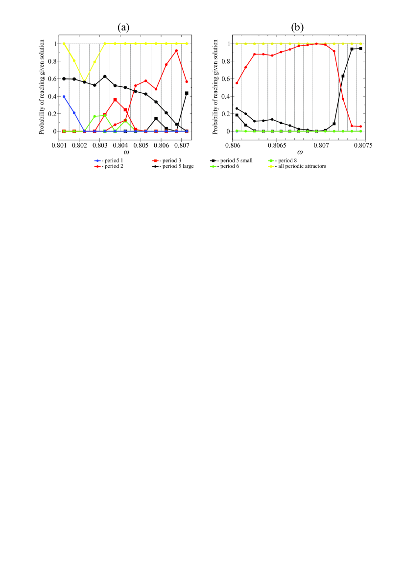
Figure 8: Probability of reaching given solutions in the impacting system. Subplots (a,b) present different periodic solutions and the summary probability of reaching any periodic solution. In Subplot (a) we analyze $\omega\in[0.801,\>0.8075]$ with the step $\Delta\omega=0.0005$, and in subplot (b) we narrow the range $\omega\in[0.806,\>0.8075]$ and decrease the step size $\Delta\omega=0.0001$. (Please note that in cases (a) and (b) the initial conditions and parameter are somehow random, hence the results may slightly differ).

4.3 Beam with suspended rotating pendula

The third considered system consists of a beam that can move horizontally with two ($n=2$) or twenty ($n=20$) pendula suspended on it. As a control parameter we use $k_{x}$ which describes the stiffness of the beam’s support. For the considered range of $k_{x}\in[100,\,5000]$ two stable periodic attractors exist in that system. One corresponds to complete synchronization of the rotating pendula. The second one is called anti-phase synchronization and refers to the state when the pendula rotate in the same direction but are shifted in phase by $\pi$.

In Figure 9 we show four bifurcation diagrams with $k_{x}$ as the controlling parameter and a Pioncare map of rotational speed of the pendula. The subplots (a,b) refer to the system with two pendula ($n=2$). We start with zero initial conditions: $x_{0}=0.0$, $\dot{x}_{0}=0.0$, $\varphi_{10}=0.0$, $\dot{\varphi}_{10}=0.0$, $\varphi_{20}=0.0$, $\dot{\varphi}_{20}=0.0$ and take $k_{x}\in[100,\,5000]$. The parameter $k_{x}$ is increasing in subplot (a) and decreasing in (b). We see that in the range marked by grey rectangle both complete and anti-phase synchronization coexist. In subplots (c,d) we present results for twenty pendula ($n=20$). We start the integration from initial conditions that refer to anti-phase synchronization (two clusters of 10 pendula shifted by $\pi$) i.e. $x_{0}=0.1$, $\dot{x}_{0}=0.00057$, $\varphi_{k0}=0.0$, $\dot{\varphi}_{k0}=9.81$, $\varphi_{j0}=3.09$, $\dot{\varphi}_{j0}=9.784$ where: $k=1,2,\ldots 10$ and $j=11,12,\ldots 20$. The value of $k_{x}$ is increasing in subplot (c) and decreasing in (d). Similarly as in the two pendula case, we observe the region ($k_{x}\in[100,\,750]$) where two solutions coexist: anti-phase synchronization and non-synchronous state. To further analyse multistability in that system we use proposed method.

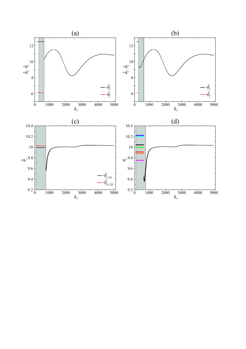
Figure 9: Bifurctaion diagram showing the behaviour of two (a,b) and twenty (c,d) pendula suspended on the moving beam. For subplots (a,c) the value of the bifurcation parameter $k_{x}$ was increased, while for subplots (b,d) we decreased the value of $k_{x}$. Grey rectangles mark the ranges of the bifurcation parameter $k_{x}$ for which different attractors coexist. Further analysis of number of solutions can be found in [13].

In Figure 10 we present how the probability of reaching a given solution depends on the parameter $k_{x}$ . In subplot (a) we show the results for the system with 2 pendula, while in subplot (b) results obtained for the system with 20 pendula suspended on the beam are given. In both cases we consider $k_{x}\in[0,\>5000]$ and assume the following ranges of initial conditions: $x_{0}\in[-0.15,\>0.15]$, $\dot{x}_{0}\in[-0.1,\>0.1]$, $\varphi_{i0}\in[-\pi,\>\pi]$, $\varphi_{20}\in[-\pi,\>\pi]$, $\dot{\varphi}_{10}\in[-3.0,\>3.0]$ and $\dot{\varphi}_{20}\in[-3.0,\>3.0]$ in Figure 10(a) and $x_{0}\in[-0.15,\>0.15]$, $\dot{x}_{0}\in[-0.1,\>0.1]$, $\varphi_{i0}\in[-\pi,\>\pi]$, $\dot{\varphi}_{i0}\in[-\pi,\>\pi]$ where $i=1\dots\>20$ in Figure 10(b). We take $20$ subsets of parameter $k_{x}$ values with the step equal to $\Delta k_{x}=250$ and mark their borders with vertical lines. For each set we run $N=100$ simulations; each one with random initial conditions and $k_{x}$value drawn from the respective subset. Then, we estimate the probability of reaching given solution. The dots in Figure 10 indicate the probability of reaching a given solution in the considered range (dots are drawn for mean value, i.e, middle of subset). Contrary to both already presented systems, this one has a much larger dimension of phase space (six and forty two), hence we decide to decrease number of the trials to $N=100$ in order to minimise the time of calculations.

In Figure 10(a) we show the results for 2 pendula. When $k_{x}\in[0,\>250]$ only anti-phase synchronization is possible. Then, with the increase of $k_{x}$ we observe a sudden change in the probability and for $k_{x}\in[750,\>1750]$ only complete synchronization exists. For $k_{x}>2000$ a probability of reaching both solutions fluctuates around $p(\mathrm{complete})=0.7$ for complete and $p(\mathrm{\mathrm{anti-phas}e})=0.3$ for anti-phase synchronization. Further increase of $k_{x}$ does not introduce any significant changes.

In Figure 10(b) we show the results for twenty pendula. For $k_{x}\in[0,\>250]$ the system reaches solutions different from the two analysed (usually chaotic). Then, the probability of reaching complete synchronization drastically increases and for $k_{x}\in[750,\>5000]$ it is equal to $p(complete)=1.0$ which means that the pendula always synchronize completely. We also present the magnification of the plot where we see that in fact for $k_{x}\in[715,\>5000]$ we will always observe complete synchronization of the pendula. Please note that for calculating both plots we use random initial conditions and $k_{x}$ value hence, the results for a narrower range may differ. Anti-phase synchronization was never achieved with randomly chosen initial conditions. This means that even though this solution is stable for $k_{x}\in[100,\>750]$ (see Figure 9(c)) it has a much smaller basin of attraction and is extremely hard to obtain in reality. The results presented in Figure10 prove that by proper tuning of the parameter $k_{x}$ we can control the systems behaviour even if we can only fix the $k_{x}$ value with finite precision.

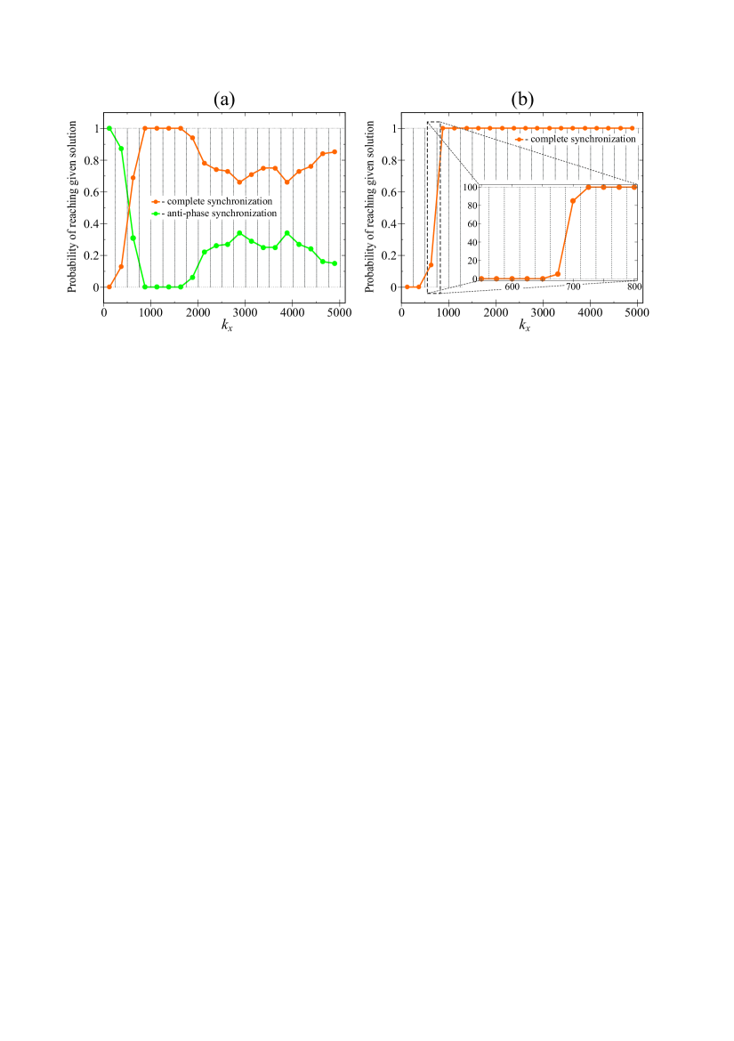
Figure 10: Probability of reaching given solutions in the system with rotating pendula. Subplot (a) refers to the case with two pendula and (b) with twenty pendula. (Please note that on plot (b) and its magnification the initial conditions and parameter are somehow random, hence the results may slightly differ).

5 Conclusions

In this paper we propose a new method of detection of solutions’ in non-linear mechanical or structural systems. The method allows to get a general view of the system’s dynamics and estimate the risk that the system will behave behave differently than assumed. To achieve this goal we extend the method of basin stability [23]. We build up the classical algorithm and draw not only initial conditions but also values of system’s parameters. We take this into account because the identification of parameters’ values is quite often not very precise. Moreover values of parameters often slowly vary during operation. Whereas in practical applications we usually need certainty that the presumed solution is stable and its basin of stability is large enough to ensure its robustness. Hence, there is a need to describe how small changes of parameters’ values influence the behaviour of the system. Our method provides such a description and allows us to estimate the required accuracy of parameters values and the risk of unwanted phenomena. Moreover it is relatively time efficient and does not require high computational power.

We show three examples, each for a different class of systems: a tuned mass absorber, a piecewise smooth oscillator and a multi-degree of freedom system. Using the proposed method we can estimate the number of existing solutions, classify them and predict their probability of appearance. Nevertheless, in many cases it is not necessary to distinct all solutions existing in a system but it is enough to focus on an expected solution, while usually other periodic, quasi-periodic and chaotic solutions are classified as undesirable. Such a strategy simplifies the analysis and reduces the computational effort. We can focus only on probable solutions and reduce the number of trials omitting a precise description of solutions with low probability.

The proposed method is robust and can be used not only for mechanical and structural systems but also for any system given by differential equations where the knowledge about existing solutions is crucial.

Appendix A

The motion of the system presented in Figure 3 is described by the following set of two second order ODEs:

$$m_{iD}l_{D}^{2}\ddot{\varphi^{\prime}}_{i}+m_{iD}\ddot{x^{\prime}}l_{D}\cos{\varphi^{\prime}_{i}}+c_{\varphi D}\dot{\varphi^{\prime}}_{i}+m_{iD}g_{D}l_{D}\sin{\varphi^{\prime}_{i}}=N_{0D}-\dot{\varphi^{\prime}}_{i}N_{1D}$$ (4)

$$\left({M_{D}+\sum\limits_{i=1}^{n}{m_{iD}}}\right)\ddot{x^{\prime}}+c_{xD}\dot{x^{\prime}}+k_{xD}x^{\prime}=\sum\limits_{i=1}^{n}{m_{iD}l_{D}\left({-\ddot{\varphi^{\prime}}_{i}\cos\varphi^{\prime}_{i}+\dot{\varphi^{\prime}}_{i}^{2}\sin\varphi^{\prime}_{i}}\right)}$$ (5)

The values of parameters and their dimensions are as follow: $m_{iD}=\frac{2.00}{n}\,[kg]$, $l_{D}=0.25\,[m]$, $c_{\varphi D}=\frac{0.02}{n}\,[Nms]$, $N_{0D}=5.00\,[Nm]$, $N_{1D}=0.50\,[Nms]$, $M_{D}=6.00\,[kg]$, $g_{D}=9.81\,[\frac{m}{s^{2}}]$, $c_{x_{D}}=\frac{\ln\left(1.5\right)}{\pi}\sqrt{k_{x}\left(M+\sum\limits_{i=1}^{n}{m_{i}}\right)}\,[\frac{Ns}{m}]$ and $k_{xD}\,[\frac{N}{m}]$ is controlling parameter. The derivation of the above equations can be found in [13]. We perform a transformation to a dimensionless form in a way that enables us to hold parameters’ values. It is because we want to present new results in a way that thay can be easily compared to results of the investigation presented in [13]. We introduce dimensionless time $\tau=t\omega_{0}$, where $\omega_{0}=1\,\mathrm{[Hz]}$, and unit parameters $m_{0}=1.0\,[kg]$, $l_{0}=1.0\,[m]$ and reach the dimensionless equations:

$$m_{i}l^{2}\ddot{\varphi}_{i}+m_{i}\ddot{x}l\cos{\varphi_{i}}+c_{\varphi}\dot{\varphi}_{i}+m_{i}gl\sin{\varphi_{i}}=N_{0}-\dot{\varphi}_{i}N_{1}$$ (6)

$$\left({M+\sum\limits_{i=1}^{n}{m_{i}}}\right)\ddot{x}+c_{x}\dot{x}+k_{x}x=\sum\limits_{i=1}^{n}{m_{i}l\left({-\ddot{\varphi}_{i}\cos\varphi_{i}+\dot{\varphi}_{i}^{2}\sin\varphi_{i}}\right)}$$ (7)

where: $x=\frac{x^{\prime}}{l_{0}}$, $\dot{x}=\frac{\dot{x^{\prime}}}{l_{0}\omega_{0}}$, $\ddot{x}=\frac{\ddot{x^{\prime}}}{l_{0}\omega_{0}^{2}}$, $\varphi_{i}=\varphi^{\prime}_{i}$, $\dot{\varphi}_{i}=\frac{\dot{\varphi^{\prime}}_{i}}{\omega_{0}}$, $\ddot{\varphi}_{i}=\frac{\ddot{\varphi^{\prime}}_{i}}{\omega_{0}^{2}}$, $m_{i}=\frac{m_{iD}}{m_{0}}$, $l=\frac{l_{D}}{l_{0}}$, $c_{\varphi}=\frac{c_{\varphi D}}{m_{0}l_{o}^{2}\omega_{0}}$, $N_{0}=\frac{N_{0D}}{m_{0}l_{o}^{2}\omega_{0}^{2}}$, $N_{1}=\frac{N_{1D}}{m_{0}l_{o}^{2}\omega_{0}}$, $M=\frac{M_{D}}{m_{0}}$, $g=\frac{g_{D}}{l_{o}\omega_{0}^{2}}$, $c_{x}=\frac{c_{xD}}{m_{0}\omega_{0}}$ and dimensionless control parameter $k_{x}=\frac{k_{xD}}{m_{0}\omega_{0}^{2}}$. Dimensionless parameters have the following values: $m_{i}=\frac{2.0}{n}$, $l=0.25$, $c_{\varphi}=\frac{0.02}{n}$, $N_{0}=5.0$, $N_{1}=0.5$, $M=6.0$, $g=9.81$.

References

- [1] A.S. Alsuwaiyan and S.W. Shaw. Performance and dynamics stability of general-path centrifugal pendulum vibration absorbers. Journal of Sound and Vibration, 252(5):791–815, 2002.
- [2] F. R. Arnold. Steady-state behavior of systems provided with nonlinear dynamic vibration absorbers. Journal of Applied Mathematics, 22:487–492, 1955.
- [3] A. Beléndez, A. Hernández, A. Márquez, T. Beléndez, and C. Neipp. Analytical approximations for the period of a nonlinear pendulum. European Journal of Physics, 27(3):539, 2006.
- [4] B. Blazejczyk-Okolewska and T. Kapitaniak. Co-existing attractors of impact oscillator. Chaos, Solitons & Fractals, 9(8):1439–1443, 1998.
- [5] P. Brzeski, T. Kapitaniak, and P. Perlikowski. Analysis of transitions between different ringing schemes of the church bell. International Journal Of Impact Engineering, 86:57 – 66, 2015.
- [6] P. Brzeski, P. Perlikowski, and T. Kapitaniak. Numerical optimization of tuned mass absorbers attached to strongly nonlinear duffing oscillator. Communications in Nonlinear Science and Numerical Simulation, 19(1):298 – 310, 2014.
- [7] P. Brzeski, P. Perlikowski, S. Yanchuk, and T. Kapitaniak. The dynamics of the pendulum suspended on the forced duffing oscillator. Journal of Sound and Vibration, 331:5347–5357, 2012.
- [8] S.L. Bux and J.W. Roberts. Non-linear vibratory interactions in systems of coupled beams. Journal of Sound and Vibration, 104(3):497–520, 1986.
- [9] M. Cartmell and J. Lawson. Performance enhancement of an autoparametric vibration absorber by means of computer control. Journal of Sound and Vibration, 177(2):173–195, 1994.
- [10] M.P. Cartmell and J.W. Roberts. Simultaneous combination resonances in an autoparametrically resonant system. Journal of Sound and Vibration, 123(1):81–101, 1988.
- [11] A. Chudzik, Przemyslaw Perlikowski, Andrzej Stefanski, and Tomasz Kapitaniak. Multistability and rare attractors in van der pol-duffing oscillator. I. J. Bifurcation and Chaos, 21(7):1907–1912, 2011.
- [12] L. L. Chung, L. Y. Wu, K. H. Lien, H. H. Chen, and H. H. Huang. Optimal design of friction pendulum tuned mass damper with varying friction coefficient. Structural Control and Health Monitoring, 2012.
- [13] K. Czolczynski, P. Perlikowski, A. Stefanski, and T. Kapitaniak. Synchronization of slowly rotating pendulums. International Journal of Bifurcation and Chaos, 22(05), 2012.
- [14] S. L. T. de Souza and I. L. Caldas. Basins of attraction and transient chaos in a gear-rattling model. Journal of vibration and control, 7(6):849–862, 2001.
- [15] S. L. T. de Souza and I. L. Caldas. Controlling chaotic orbits in mechanical systems with impacts. Chaos, Solitons & Fractals, 19(1):171–178, 2004.
- [16] U. Feudel, C. Grebogi, L. Poon, and J. A. Yorke. Dynamical properties of a simple mechanical system with a large number of coexisting periodic attractors. Chaos, Solitons & Fractals, 9(1):171–180, 1998.
- [17] O. Fischer. Wind-excited vibrations - solution by passive dynamic vibration absorbers of different types. Journal of Wind Engineering and Industrial Aerodynamics, 95(9):1028–1039, 2007.
- [18] Y. Gerson, S. Krylov, B. Ilic, and D. Schreiber. Design considerations of a large-displacement multistable micro actuator with serially connected bistable elements. Finite Elements in Analysis and Design, 49(1):58–69, 2012.
- [19] N. HaQuang, D. T. Mook, and R. H. Plaut. Non-linear structural vibrations under combined parametric and external excitations. Journal of Sound and Vibration, 118(2):291–306, 1987.
- [20] J-H. He. The homotopy perturbation method for nonlinear oscillators with discontinuities. Applied Mathematics and Computation, 151(1):287–292, 2004.
- [21] T. Ikeda. Bifurcation phenomena caused by multiple nonlinear vibration absorbers. Journal of Computational and Nonlinear Dynamics, 5:021012, 2010.
- [22] V. V. Klinshov, V. I. Nekorkin, J. Kurths. Stability threshold approach for complex dynamical systems New J. Physics, 18:013004, 2016.
- [23] P. J. Menck, J. Heitzig, N. Marwan, and J. Kurths. How basin stability complements the linear-stability paradigm. Nature Physics, 9(2):89–92, 2013.
- [24] A. H. Nayfeh. Introduction to perturbation techniques. John Wiley & Sons, 2011.
- [25] A. H. Nayfeh and P. F. Pai. Linear and nonlinear structural mechanics. John Wiley & Sons, 2008.
- [26] D. Orlando, P. B. Gonçalves, G. Rega, and S. Lenci. Influence of symmetries and imperfections on the non-linear vibration modes of archetypal structural systems. International Journal of Non-Linear Mechanics, 49:175–195, 2013.
- [27] E. Pavlovskaia, J. Ing, M. Wiercigroch, and S. Banerjee. Complex dynamics of bilinear oscillator close to grazing. International Journal of Bifurcation and Chaos, 20(11):3801–3817, 2010.
- [28] L. Qun-hong and L. Qi-shao. Coexisting periodic orbits in vibro-impacting dynamical systems. Applied Mathematics and Mechanics, 24(3):261–273, 2003.
- [29] S. S. Rao and F. F. Yap. Mechanical vibrations, volume 4. Addison-Wesley Reading, 1995.
- [30] B. Vazquez-Gonzalez and G. Silva-Navarro. Evaluation of the autoparametric pendulum vibration absorber for a duffing system. Shock and Vibration, 15:355–368, 2008.
- [31] J. Warminski, G. Litak, M. P. Cartmell, R. Khanin, and M. Wiercigroch. Approximate analytical solutions for primary chatter in the non-linear metal cutting model. Journal of Sound and Vibration, 259(4):917–933, 2003.
- [32] S. Yanchuk, P. Perlikowski, O. V. Popovych, and P. A. Tass. Variability of spatio-temporal patterns in non-homogeneous rings of spiking neurons. Chaos, 21:047511, 2011.