Strongly Near Voronoï Nucleus Clusters

Abstract.

This paper introduces nucleus clustering in Voronoï tessellations of plane surfaces with applications in the geometry of digital images. A nucleus cluster is a collection of Voronoï regions that are adjacent to a Voronoï region called the cluster nucleus. Nucleus clustering is a carried out in a strong proximity space. Of particular interest is the presence of maximal nucleus clusters in a tessellation. Among all of the possible nucleus clusters in a Voronoï tessellation, clusters with the highest number of adjacent polygons are called maximal nucleus clusters. The main results in this paper are that strongly near nucleus clusters are strongly descriptively near and every collection of Voronoï regions in a tessellation of a plane surface is a Zelins’kyi-Soltan-Kay-Womble convexity structure.

1. Introduction

This paper introduces nucleus clustering in Voronoï tessellations of surfaces in Euclidean space $\mathbb{R}^{d},d\geq 2$. In this article, nucleus clustering is restricted to plane surfaces with applications in the geometry of digital images. A nucleus cluster is a collection of Voronoï regions that are adjacent to a Voronoï region called the cluster nucleus, which is a variation of the notion of a Harer-Edelsbrunner nerve [6, §III.2, p. 59].

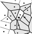
Figure 1.
Nucleus Cluster

Every Voronoï region of a site $s$ is a convex polygon containing all points that are nearer $s$ than to any other site in a Voronoï tessellation of a surface. Voronoï regions are strongly near, provided the regions have points in common. This form of clustering leads to the introduction of what are known as nucleus-clusters. A nucleus cluster is a collection of Voronoï regions that are strongly near a central Voronoï region called the cluster nucleus in a Voronoï tessellation. A maximal nucleus cluster is a collection of a maximal number of Voronoï regions that are strongly near the mesh nucleus. Maximal nucleus clusters serve as indicators of high object concentration in a tessellated image. This form of clustering leads to object recognition in many forms of application images.

2. Preliminaries

This section introduces strongly near proximity and Voronoï tessellation of a plane surface based on recent work on computational proximity [14], computational geometry [3, 4, 5, 6]. Strong proximities were introduced in [16], elaborated in [14] (see, also, [8]) and are a direct result of earlier work on proximities [1, 2, 10, 11, 12]. Nonempty sets $A$ and $B$ have strong proximity (denoted $A\ \mathop{\delta}\limits^{\doublewedge}\ B$), provided $A$ and $B$ have points in common. Let $E$ be the Euclidean plane, $S\subset E$ (set of mesh generating points), $s\in S$. A Voronoï region (denoted by $V(s)$) is defined by

$$V(s)=\left\{x\in E:\left\|x-s\right\|\leq\left\|x-q\right\|,\mbox{for all}\ q\in S\right\}\ \mbox{(Vorono\"{i} region)}.$$

Example 1.

A partial view of a Voronoï tessellation of a plane surface is shown in Fig. 1. The Voronoï region $N$ in this tessellation is the nucleus of a mesh clustering containing all of those polygons adjacent to $N$. Let $X$ be a collection of Voronoï regions containing $N$, endowed with the strong proximity $\mathop{\delta}\limits^{\doublewedge}$. Briefly, a proximity relation is strong, provided $A\ \mathop{\delta}\limits^{\doublewedge}\ B,A,B\in X$ have points in common. Then the nucleus mesh cluster (denoted by $\mbox{\large$\mathfrak{C}$}\ N$) in this sample tessellation is defined by

$$\mbox{\large$\mathfrak{C}$}\ N=\left\{A\in X:\mathop{\mbox{cl}}\limits^{\doublewedge}\ A\ \mathop{\delta}\limits^{\doublewedge}\ N\right\}\ \mbox{(Vorono\"{i} mesh nucleus cluster)}.\\$$

That is, a nucleus mesh cluster $\mbox{\large$\mathfrak{C}$}\ N$ is a collection of nonempty sets $A$ whose closure is strongly near the cluster nucleus $N$ (in that case, each $A\in\mbox{\large$\mathfrak{C}$}\ N$ has points in common with $N$). For example, the set of points in the convex polygon $N$ in Fig. 1 has points in common with each of the adjacent polygons, i.e., each polygon adjacent to $N$ has an edge in common with $N$. Let $B$ be a polygon adjacent to $N$. $B\ \mathop{\delta}\limits^{\doublewedge}\ N$, since $B$ and $N$ have in edge in common.   ◼

A concrete (physical) set $A$ of points $p$ that are described by their location and physical characteristics, e.g., gradient orientation (angle of the tangent to $p$. Let $\varphi(p)$ be the gradient orientation of $p$. For example, each point $p$ with coordinates $(x,y)$ in the concrete subset $A$ in the Euclidean plane is described by a feature vector of the form $(x,y,\varphi(p(x,y))$. Nonempty concrete sets $A$ and $B$ have descriptive strong proximity (denoted $A\ \mathop{\delta_{{}_{\Phi}}}\limits^{\doublewedge}\ B$), provided $A$ and $B$ have points with matching descriptions. In a region-based, descriptive proximity extends to both abstract and concrete sets [14, §1.2]. For example, every subset $A$ in the Euclidean plane has features such as area and diameter. Let $(x,y)$ be the coordinates of the centroid $m$ of $A$. Then $A$ is described by feature vector of the form $(x,y,area,diameter)$. Then regions $A,B$ have descriptive proximity (denoted $A\ \mathop{\delta_{{}_{\Phi}}}\limits^{\doublewedge}\ B$), provided $A$ and $B$ have matching descriptions.

The notion of strongly proximal regions extends to convex sets. A nonempty set $A$ is a convex set (denoted $\mbox{conv}A$), provided, for any pair of points $x,y\in A$, the line segment $\overline{xy}$ is also in $A$. The empty set $\emptyset$ and a one-element set $\left\{x\right\}$ are convex by definition. Let $\mathscr{F}$ be a family of convex sets. From the fact that the intersection of any two convex sets is convex [5, §2.1, Lemma A], it follows that

$$\mathop{\bigcap}\limits_{A\in\mathscr{F}}A\ \mbox{is a convex set}.$$

Convex sets $\mbox{conv}A,\mbox{conv}B$ are strongly proximal (denote $\mbox{conv}A\mathop{\delta}\limits^{\doublewedge}\ \mbox{conv}B$), provided $\mbox{conv}A,\mbox{conv}B$ have points in common. Convex sets $\mbox{conv}A,\mbox{conv}B$ are descriptively strongly proximal (denoted $\mbox{conv}A\mathop{\delta_{{}_{\Phi}}}\limits^{\doublewedge}\ \mbox{conv}B$), provided $\mbox{conv}A,\mbox{conv}B$ have matching descriptions.

Let $X$ be a Voronoï tessellation of a plane surface equipped with the strong proximity $\mathop{\delta}\limits^{\doublewedge}$ and descriptive strong proximity $\mathop{\delta_{{}_{\Phi}}}\limits^{\doublewedge}$ and let $A,N\in X$ be Voronoï regions. The pair $\left(X,\left\{\mathop{\delta}\limits^{\doublewedge},\mathop{\delta_{{}_{\Phi}}}\limits^{\doublewedge}\right\}\right)$ is an example of a proximal relator space [17]. The two forms of nucleus clusters (ordinary nucleus cluster denoted by $\mathfrak{C}$) and descriptive nucleus clusters are examples of mesh nerves [14, §1.10, pp. 29ff], defined by

$$\mbox{\large$\mathfrak{C}$}N =\left\{A\in X:A\ \mathop{\delta}\limits^{\doublewedge}\ N\right\}\ \mbox{(nucleus cluster)}.$$

$$\mathfrak{C}_{\Phi}N =\left\{A\in X:A\ \mathop{\delta_{{}_{\Phi}}}\limits^{\doublewedge}\ N\right\}\ \mbox{(descriptive nucleus cluster)}.$$

A nucleus cluster is maximal (denoted by $\mbox{max}\mathfrak{C}N$), provided $N$ has the highest number of adjacent polygons in a tessellated surface (more than one maximal cluster in the same mesh is possible). Similarly, a descriptive nucleus cluster is maximal (denoted by $\mbox{max}\mathfrak{C}_{\Phi}N$), provided $N$ has the highest number of polygons in a tessellated surface descriptively near $N$, i.e., the description of each $A\in\mbox{max}\mathfrak{C}_{\Phi}N$ matches the description of nucleus $N$ and the number of polygons descriptively near $N$ is maximal (again, more than one $\mbox{max}\mathfrak{C}_{\Phi}N$ is possible in a Voronoï tessellation).

Figure 2. $\mbox{\large$\mathfrak{C}$}\ N_{1}\ \mathop{\delta}\limits^{\doublewedge}\ \mbox{\large$\mathfrak{C}$}\ N_{2}\ \mbox{and}\ \mbox{\large$\mathfrak{C}$}\ N_{2}\ \mathop{\delta}\limits^{\doublewedge}\ \mbox{\large$\mathfrak{C}$}\ N_{3}$

Example 2.

Let $X$ the collection of Voronoï regions shown in Fig. 2 with $N_{1},N_{2},N_{3}\in X$. In addition, let $2^{X}$ be the family of all subsets of Voronoï regions in $X$. Then $\mbox{\large$\mathfrak{C}$}N_{1},\mbox{\large$\mathfrak{C}$}N_{2},\mbox{\large$\mathfrak{C}$}N_{3}\in 2^{X}$ nucleus clusters in the tessellation. In this sample plane surface tessellation, $\mbox{\large$\mathfrak{C}$}N_{1}\ \mathop{\delta}\limits^{\doublewedge}\ \mbox{\large$\mathfrak{C}$}N_{2}$, since $A\ \mathop{\delta}\limits^{\doublewedge}\ B$ for some $A\in\mbox{\large$\mathfrak{C}$}N_{1},B\in\mbox{\large$\mathfrak{C}$}N_{2}$. Similarly, $\mbox{\large$\mathfrak{C}$}N_{2}\ \mathop{\delta}\limits^{\doublewedge}\ \mbox{\large$\mathfrak{C}$}N_{3}$. In addition, nucleus clusters $\mbox{\large$\mathfrak{C}$}N_{2},\mbox{\large$\mathfrak{C}$}N_{3}$ are maximal (denoted by $\mbox{max}\mathfrak{C}N_{2},\mbox{max}\mathfrak{C}N_{3}$), since nuclei $N_{2},N_{3}$ in the tessellation have the maximal number of adjacent Voronoï regions, namely, 10 adjacent regions. Let the description of a nucleus cluster in the Euclidean plane be described by its number of sides of its nucleus. Then $\mbox{max}\mathfrak{C}N_{2}\ \mathop{\delta_{{}_{\Phi}}}\limits^{\doublewedge}\ \mbox{max}\mathfrak{C}N_{3}$, since $N_{2}\ \mathop{\delta_{{}_{\Phi}}}\limits^{\doublewedge}\ N_{3}$, i.e., the description of $N_{2}$ strongly matches the description of $N_{3}$ inasmuch as the description of the one nucleus is contained in the description of the other nucleus. In a more complete description, we would also consider the gradient orientation of the nucleus edges. In the case, $N_{2}\ \mathop{\delta_{{}_{\Phi}}}\limits^{\doublewedge}\ N_{3}$, provided each nucleus has at least one edge with a gradient orientation that matches the gradient orientation of an edge in the other nucleus.   ◼

Theorem 1.

Let $X$ be a set of Voronoï regions in the tessellation of a plane surface, endowed with the proximities $\mathop{\delta}\limits^{\doublewedge},\mathop{\delta_{{}_{\Phi}}}\limits^{\doublewedge},\delta_{\Phi}$ with $A,N\in X$. In addition, let $2^{X}$ be the family of all subsets of Voronoï regions in $X$. Then

1. $A\in X$ implies $A\in\mbox{\large$\mathfrak{C}$}N$ for some $N\in X$.

2. $\mbox{\large$\mathfrak{C}$}N\in 2^{X}$ implies $A\ \mathop{\delta}\limits^{\doublewedge}\ N$ for some $A\in X$.

3. The union of all Voronoï nucleus clusters cover a plane surface, i.e.,

   $$X=\mathop{\bigcup}\limits_{N\in X}\mbox{\large$\mathfrak{C}$}N\ \mbox{(Nucleus cluster covering property)}.$$

4. $N,N^{\prime}\in X$ implies $\mbox{\large$\mathfrak{C}$}N,\mbox{\large$\mathfrak{C}$}N^{\prime}\in 2^{X}$.

5. Let the description of $N\in X$ be the number of edges on the polygon $N$. Then
   $\mbox{max}\mathfrak{C}N,\mbox{max}\mathfrak{C}N^{\prime}\in 2^{X}$ implies $N\ \mathop{\delta_{{}_{\Phi}}}\limits^{\doublewedge}\ N^{\prime}$ for $N,N^{\prime}\in X$.

6. $\mbox{\large$\mathfrak{C}$}N\ \mathop{\delta}\limits^{\doublewedge}\ \mbox{\large$\mathfrak{C}$}N^{\prime}$, if and only $A\ \mathop{\delta}\limits^{\doublewedge}\ B$ for some $A\in\mbox{\large$\mathfrak{C}$}N,B\in\mbox{\large$\mathfrak{C}$}N^{\prime}$.

7. $\mbox{\large$\mathfrak{C}$}N\ \mathop{\delta_{{}_{\Phi}}}\limits^{\doublewedge}\ \mbox{\large$\mathfrak{C}$}N^{\prime}$, if and only if $A\ \mathop{\delta_{{}_{\Phi}}}\limits^{\doublewedge}\ B$ for some $A\in\mbox{\large$\mathfrak{C}$}N,B\in\mbox{\large$\mathfrak{C}$}N^{\prime}$.

8. $A\ \mathop{\delta}\limits^{\doublewedge}\ \mbox{\large$\mathfrak{C}$}\ B$, for $A\in X,\mbox{\large$\mathfrak{C}$}\ B\in 2^{X}$ implies $\mbox{\large$\mathfrak{C}$}N\ \mathop{\delta}\limits^{\doublewedge}\ \mbox{\large$\mathfrak{C}$}B$ for some $N\in X$, where $A\ \mathop{\delta}\limits^{\doublewedge}\ N$.

9. $\mbox{\large$\mathfrak{C}$}N\ \cap\ \mbox{\large$\mathfrak{C}$}N^{\prime}\neq\emptyset$ implies $A\ \mathop{\delta}\limits^{\doublewedge}\ B$ for some $A\in\mbox{\large$\mathfrak{C}$}N,B\in\mbox{\large$\mathfrak{C}$}N^{\prime}$.

10. Let $\mbox{\large$\mathfrak{C}$}N\ \mathop{\cap}\limits_{\Phi}\ \mbox{\large$\mathfrak{C}$}N^{\prime}=\left\{A\in\mbox{\large$\mathfrak{C}$}N\cup\mbox{\large$\mathfrak{C}$}N^{\prime}:A\in\Phi(\mbox{\large$\mathfrak{C}$}N)\ \&\ A\in\Phi(\mbox{\large$\mathfrak{C}$}N^{\prime})\right\}$ (descriptive intersection of nucleus clusters). Then $\mbox{\large$\mathfrak{C}$}N\ \mathop{\cap}\limits_{\Phi}\ \mbox{\large$\mathfrak{C}$}N^{\prime}\neq\emptyset$ implies $A\ \delta_{\Phi}\ B$ for some $A\in\mbox{\large$\mathfrak{C}$}N,B\in\mbox{\large$\mathfrak{C}$}N^{\prime}$.

Proof.

We prove only 6^o and 7^o. The proof of the remaining parts are direct consequences of the definitions.
6^o: $A\ \mathop{\delta}\limits^{\doublewedge}\ B$ ($A$ and $B$ have a common edge) for some $A\in\mbox{\large$\mathfrak{C}$}N,B\in\mbox{\large$\mathfrak{C}$}N^{\prime}$, if and only if $\mbox{\large$\mathfrak{C}$}N,\mbox{\large$\mathfrak{C}$}N^{\prime}$ are adjacent, if and only if $\mbox{\large$\mathfrak{C}$}N\ \mathop{\delta}\limits^{\doublewedge}\ \mbox{\large$\mathfrak{C}$}N^{\prime}$.
7^o: $A\ \mathop{\delta_{{}_{\Phi}}}\limits^{\doublewedge}\ B$ for some $A\in\mbox{\large$\mathfrak{C}$}N,B\in\mbox{\large$\mathfrak{C}$}N^{\prime}$, if and only if the description of $A$ matches the description of $B$ ($A,B$ can be either adjacent or non-adjacent), if and only if $\mbox{\large$\mathfrak{C}$}N\ \cap\ \mbox{\large$\mathfrak{C}$}N^{\prime}\neq\emptyset$, if and only if, $A\ \mathop{\delta_{{}_{\Phi}}}\limits^{\doublewedge}\ B$. ∎

Remark 1.

Let $X$ be a set of Voronoï regions in the tessellation of a plane surface, endowed with the proximities $\mathop{\delta}\limits^{\doublewedge},\mathop{\delta_{{}_{\Phi}}}\limits^{\doublewedge},\delta_{\Phi}$ with $A,N\in X$. From Theorem 1.6, the nuclei in adjacent Voronoï nucleus clusters have a strong affinity in the sense that each of the clusters contains a Voronoï region that is strongly near a Voronoï region in an adjacent cluster. For example, in Fig. 2, clusters $\mbox{\large$\mathfrak{C}$}N_{1},\mbox{\large$\mathfrak{C}$}N_{2}$ share a pair of adjacent polygons. The nuclei in adjacent Voronoï nucleus clusters have a strong descriptive affinity, provided the nuclei have matching descriptions. It also the case that Voronoï regions $V(s),V(s^{\prime})\in X$ are descriptively near, provided $s\ \delta_{\Phi}\ s^{\prime}$, i.e., the description of $s$ matches the description of $s^{\prime}$. Hence, from Theorem 1.7, $\mbox{\large$\mathfrak{C}$}V(s)\ \mathop{\delta_{{}_{\Phi}}}\limits^{\doublewedge}\ \mbox{\large$\mathfrak{C}$}V(s^{\prime})$.   ◼

3. Main Results

Lemma 1.

$A\ \mathop{\delta}\limits^{\doublewedge}\ B\Rightarrow A\ \mathop{\delta_{{}_{\Phi}}}\limits^{\doublewedge}\ B$.

Proof.

$A\ \mathop{\delta}\limits^{\doublewedge}\ B$ implies that $A$ and $B$ have points in common. Hence, there are points in $A$ and $B$ with the same descripitons, i.e., $A\ \mathop{\delta_{{}_{\Phi}}}\limits^{\doublewedge}\ B$ ∎

Theorem 2.

$\mbox{\large$\mathfrak{C}$}\ N\ \mathop{\delta}\limits^{\doublewedge}\ \mbox{\large$\mathfrak{C}$}\ M\Rightarrow\mbox{\large$\mathfrak{C}$}\ N\ \mathop{\delta_{{}_{\Phi}}}\limits^{\doublewedge}\ \mbox{\large$\mathfrak{C}$}\ M$.

Proof.

Immediate from Lemma 1 and Theorem 1.7. ∎

The descriptive intersection [13, §1.9, p. 43] of nonempty sets $A,B$ (denoted $A\ \ \mathop{\cap}\limits_{\Phi}\ B$) in an $n$-dimensional Euclidean space $\mathbb{R}^{n}$ is defined in the following way.

($\boldsymbol{\Phi}$):

$\Phi(A)=\left\{\Phi(x)\in\mathbb{R}^{n}:x\in A\right\}$, set of feature vectors.

($\boldsymbol{\mathop{\cap}\limits_{\Phi}}$):

$A\ \mathop{\cap}\limits_{\Phi}\ B=\left\{x\in A\cup B:\Phi(x)\in\Phi(A)\ \&\ \Phi(x)\in\Phi(B)\right\}$.   $\blacksquare$

That is, the descriptive intersection of $A$ and $B$ contains all $a\in A,b\in B$ that are descriptively near each other.

Theorem 3.

$\mathfrak{C}_{\Phi}N\ \mathop{\delta}\limits^{\doublewedge}\ \mathfrak{C}_{\Phi}M\Leftrightarrow A\ \mathop{\cap}\limits_{\Phi}\ B\neq\emptyset$ for some $A\in{\mathop{\mathfrak{C}}\limits^{\doublewedge}}_{\Phi}\ N,B\in{\mathop{\mathfrak{C}}\limits^{\doublewedge}}_{\Phi}\ M$.

Proof.

$\mathfrak{C}_{\Phi}N\ \mathop{\delta}\limits^{\doublewedge}\ \mathfrak{C}_{\Phi}M\Leftrightarrow\mbox{\large$\mathfrak{C}$}N\ \mathop{\delta_{{}_{\Phi}}}\limits^{\doublewedge}\ \mbox{\large$\mathfrak{C}$}M\ \mbox{(from the definition of $\mathop{\delta_{{}_{\Phi}}}\limits^{\doublewedge}$)}\ \Leftrightarrow A\ \mathop{\delta_{{}_{\Phi}}}\limits^{\doublewedge}\ B$ for some $A\in\mbox{\large$\mathfrak{C}$}N,B\in\mbox{\large$\mathfrak{C}$}M$ (from Theorem 1.7), if and only if $A\ \mathop{\cap}\limits_{\Phi}\ B\neq\emptyset$. ∎

Definition 1.

Zelins’kyi-Soltan-Kay-Womble Convexity Structure[18, 21, 9]. Let $\mathscr{F}=2^{X}$ be the family of all subsets of a nonempty set $X$ and let subfamilies $\mathscr{A},\mathscr{B}\in\mathscr{F}$. The family $\mathscr{F}$ on $X$ is called a Zelins’kyi-Soltan-Kay-Womble convexity structure, provided it satisfies the following axioms.

(C0):

$\emptyset$ and $X$ belong to $\mathscr{F}$.

(C1):

$\mathscr{A}\ \cap\ \mathscr{B}\in\mathscr{F}$ for all subfamilies $\mathscr{A},\mathscr{B}\in\mathscr{F}$.   $\blacksquare$

The pair $\left(X,\mathscr{F}\right)$ is a Zelins’kyi-Soltan-Kay-Womble convexity space.

Theorem 4.

[14] The family of all subsets $\mathscr{F}=2^{X}$ of a nonempty set $X$ is a Zelins’kyi-Soltan-Kay-Womble convexity structure.

Proof.

Let $\mathcal{A}\in\mathscr{F}$. $X$ and $\emptyset$ are in $\mathscr{F}$. In addition, $\mathop{\bigcap}\limits_{A\in\mathcal{A}}A\in\mathscr{F}$. Hence, $\mathscr{F}$ is a Zelins’kyi-Soltan-Kay-Womble convexity structure. ∎

Theorem 5.

Let $X$ be a collection of Voronoï regions in the tessellation of a plane surface, $2^{X}$ the family of all subsets of $X$, $\mbox{\large$\mathfrak{C}$}N,\mbox{\large$\mathfrak{C}$}M\in 2^{X}$ such that $\mbox{\large$\mathfrak{C}$}N\cap\mbox{\large$\mathfrak{C}$}M\neq\emptyset$. The family $2^{X}$ is a Zelins’kyi-Soltan-Kay-Womble convexity structure.

Proof.

For a nonempty $X$, both $\emptyset$ and $X$ are subsets in $2^{X}$ (Axiom (C0)). Let $\mbox{\large$\mathfrak{C}$}N,\mbox{\large$\mathfrak{C}$}M$ be subcollections in $2^{X}$. $\mbox{\large$\mathfrak{C}$}N\cap\mbox{\large$\mathfrak{C}$}M\neq\emptyset$ implies that $\mbox{\large$\mathfrak{C}$}N,\mbox{\large$\mathfrak{C}$}M$ share at least one Voronoï region. Consequently, $\mbox{\large$\mathfrak{C}$}N\cap\mbox{\large$\mathfrak{C}$}M\in 2^{X}$ (Axiom (C1)). Hence, from Theorem 4, $2^{X}$ is a Zelins’kyi-Soltan-Kay-Womble convexity structure. ∎

Example 3.

From Theorem 5, the collection of Voronoï regions $\left\{\mbox{\large$\mathfrak{C}$}N_{2},\mbox{\large$\mathfrak{C}$}N_{3}\right\}$ in the tessellation shown in Fig. 2 is a convexity structure, since $\mbox{\large$\mathfrak{C}$}N_{2},\mbox{\large$\mathfrak{C}$}N_{3}$ have a Voronoï region in common.   $\blacksquare$

4. Applications

Several applications arise from the introduction of Voronoï clustering.

Satellite Images:

Detecting surface objects and locations of sharp differences in terrain. Surface objects are revealed by one or more occurrences of maximal nucleus clusters.

FMRI Images:

High cortical activity corresponds to maximal nucleus clusters in brain tissue. The leads to the detection and classification of cortical activity associated with the tessellation of fMRI images. For example, the Voronoï mesh in Fig. 2 has been extracted from the tessellation of an fMRI image of the brain. Mesh nucleus clustering is directly related to recent studies of fMRI images [19, 20].

Tomography Images:

High concentration of fossils correspond to the presence and distribution of maximal nucleus clusters in 3D tomography images derived from drill core samples.

References

• [1] A. Di Concilio, G. Gerla, Quasi-metric spaces and point-free geometry, Math. Structures Comput. Sci. 16 (2006), no. 1, 115–137, MR2220893.
• [2] A. Di Concilio, Point-free geometries: Proximities and quasi-metrics, Math. in Comp. Sci. 7 (2013), no. 1, 31-42, MR3043916.
• [3] H. Edelsbrunner, Computational Topology. Advances in discrete and computational geometry. Contemp. Math., 223, Amer. Math. Soc., Providence, RI, 1999, MR1661380.
• [4] H. Edelsbrunner, Geometry and Topology for Mesh Generation. Cambridge University Press, Cambridge, UK, 2001, 2006. xii+177 pp. ISBN: 978-0-521-68207-7; 0-521-68207-X, MR2223897.
• [5] H. Edelsbrunner, A Short Course in Computational Geometry and Topology. Springer Briefs in Applied Sciences and Technology. Springer, Cham, 2014. x+110 pp. ISBN: 978-3-319-05956-3; 978-3-319-05957-0, MR3328629.
• [6] H. Edelsbrunner, Computational Topology. An Introduction. Amer. Math. Soc., Providence, RI, 2010. xii+241 pp. ISBN: 978-0-8218-4925-5, MR2572029.
• [7] C. Guadagni, Bornological Convergences on Local Proximity Spaces and $\omega_{\mu}$-Metric Spaces, Ph.D thesis, Università degli Studi di Salerno, Dipartimento di Matematica, supervisor: A. Di Concilio, 2015, 72pp.
• [8] E. İnan, Algebraic Structures on Nearness Approximation Spaces, Ph.D thesis, İnönü University, Department of Mathematics, supervisors: S. Keleş and M.A. Öztürk, 2015, vii+113pp.
• [9] D. Kay, E. Womble, Automatic convexity theory and relationships between the carath‘eodory, helly and radon numbers, Pacific Journal of Math. 38 (1971), no. 2, 471–485.
• [10] S.A. Naimpally, B.D. Warrack, Proximity spaces, Cambridge University Press, Cambridge Tract in Mathematics and Mathematical Physics 59, Cambridge, UK, 1970, ISBN 978-0-521-09183-1, MR2573941.
• [11] S.A. Naimpally, Proximity Approach to Problems in Topology and Analysis, Oldenbourg Verlag, Munich, Germany, 2009, 73 pp., ISBN 978-3-486-58917-7, MR2526304.
• [12] S.A. Naimpally, J.F. Peters, Topology with applications. Topological spaces via near and far. With a foreword by Iskander A. Taimanov. World Scientific Publishing Co. Pte. Ltd., Hackensack, NJ, 2013. xvi+277 pp. ISBN: 978-981-4407-65-6, MR3075111.
• [13] J.F. Peters, Topology of Digital Images. Visual Pattern Discovery in Proximity Spaces. Intelligent Systems Reference Library 63, Springer (2014). DOI 10.1007/978-3-642-53845-2. URL http://dx.doi.org/10.1007/978-3-642-53845-2. XV + 411 pp. Zentralblatt MATH Zbl 1295 68010.
• [14] J.F. Peters, Computational Proximity. Excursions in the Topology of Digital Images. Springer, Intelligent Systems Reference Library, Berlin, 2016, in press.
• [15] J.F. Peters, Visibility in proximal Delaunay meshes, Advances in Math. 4 (2015), no. 1, 41-47.
• [16] J.F. Peters, C. Guadagni, Strong proximities on smooth manifolds and Vorono¨ı diagrams, Advances in Math. 4 (2015), no. 2, 97-107.
• [17] J.F. Peters, Proximal relator spaces, Filomat (2016), in press.
• [18] V.P. Soltan, Introduction to the axiomatic theory of convexity [Russian With English and French summariess, Shtiintsa, Kishinev, 1984. 224 pp., MR0779643.
• [19] A. Tozzi, J.F. Peters, Towards a fourth spatial dimension of brain activity, Cognitive Neurodynamics (2016), 1-11, DOI 10.1007/s11571-016-9379-z.
• [20] A. Tozzi, J.F. Peters, A topological approach unveils system invariances and broken symmetries in the brain, J. of Neuroscience Research (2016), 1-12, in press.
• [21] Y. Zelins’ky, Generalized convex envelopes of sets and the problem of shadow, Journal of Mathematical Sciences, 211 (2015), no. 5, 710-717.