Parallel Vertex Approximate Gradient discretization of hybrid dimensional Darcy flow and transport in discrete fracture networks

Abstract

This paper proposes a parallel numerical algorithm to simulate the flow and the transport in a discrete fracture network taking into account the mass exchanges with the surrounding matrix. The discretization of the Darcy fluxes is based on the Vertex Approximate Gradient finite volume scheme adapted to polyhedral meshes and to heterogeneous anisotropic media, and the transport equation is discretized by a first order upwind scheme combined with an Euler explicit integration in time. The parallelization is based on the SPMD (Single Program, Multiple Data) paradigm and relies on a distribution of the mesh on the processes with one layer of ghost cells in order to allow for a local assembly of the discrete systems. The linear system for the Darcy flow is solved using different linear solvers and preconditioners implemented in the PETSc and Trilinos libraries. The convergence of the scheme is validated on two original analytical solutions with one and four intersecting fractures. Then, the parallel efficiency of the algorithm is assessed on up to 512 processes with different types of meshes, different matrix fracture permeability ratios, and different levels of complexity of the fracture network.

1 Introduction

1.1 Hybrid dimensional flow and transport models

This article deals with the simulation of the Darcy flow and transport in fractured porous media for which the fractures are modeled as interfaces of codimension one. In this framework, the $d-1$ dimensional flow and transport in the fractures is coupled with the $d$ dimensional flow and transport in the matrix leading to the so called hybrid dimensional Darcy flow and transport model.

For the Darcy flow model, we focus on the particular case where the pressure is continuous at the interfaces between the fractures and the matrix domain. This type of Darcy flow model introduced in [3], [4] corresponds physically to pervious fractures for which the ratio of the normal permeability of the fracture to the width of the fracture is large compared with the ratio of the permeability of the matrix to the size of the domain. Note that it does not cover the case of fractures acting as barriers for which the pressure is discontinuous at the matrix fracture interfaces (see [22], [33], [5] for discontinuous pressure models). It is also assumed in our model that the pressure is continuous at the fracture intersections. It corresponds to the assumption that the ratio between the permeability at the fracture intersections and the width of the fracture is large compared to the ratio between the tangential permeability of each fracture and its length. We refer to [24] and [40] for more general reduced models taking into account discontinuous pressures at fracture intersections in dimension $d=2$.

The hybrid dimensional transport model is derived in [3] in the case of a convection diffusion flux for the matrix and fracture concentration. In this work, a purely advective model is considered. It requires the specification of the transmission conditions at the matrix fracture interfaces and at fracture intersections which, to our knowledge, have not been done so far at the continuous level.

The discretization of the hybrid dimensional Darcy flow model with continuous pressures has been the object of several works. In [31] a cell-centred Finite Volume scheme using a Two Point Flux Approximation (TPFA) is proposed assuming the orthogonality of the mesh and isotropic permeability fields. Cell-centred Finite Volume schemes can be extended to general meshes and anisotropic permeability fields using MultiPoint Flux Approximations (MPFA) following the ideas of [42], [39],[1] and [2]. In [3] and [29] a Mixed Finite Element (MFE) method is proposed, and Control Volume Finite Element Methods (CVFE) using nodal unknowns have been introduced for such models in [9], [38], [35], [34], [28]. The Hybrid Finite Volume and Mimetic finite difference schemes, belonging to the family of Hybrid Mimetic Mixed Methods [17], have been extended to hybrid dimensional models in [23], [6] as well as in [12], [13] in the more general Gradient Discretization framework [18]. Non-matching discretizations of the fracture and matrix meshes are studied in [16], [25], [8] and [40].

Regarding the hybrid dimensional advective transport model, an explicit first order upwind scheme combined with the MPFA Darcy fluxes is used in [1], [2], and [39]. At fracture intersections, the authors neglect the accumulation term and the concentration unknown is eliminated using the flux conservation equation in order to avoid severe restrictions on the time step caused by the small volumes. A CVFE method is used in [38] with a first order upwind approximation and a fully implicit time integration of the two phase flow model to avoid small time steps. Higher order methods have also been developed in the CVFE method of [34] using a MUSCL type second order scheme for the saturation equation and also in [29] where a Discontinuous Galerkin method is used for the transport saturation equation with an Euler implicit time integration in the fracture network and an explicit time integration in the matrix domain. In [26], a streamline method is developed in 2D based on the hybrid dimensional Darcy flow velocity field. The solution is very accurate for purely advective transport but this method requires that the fractures be expanded and seems difficult to extend to the case of a complex 3D network in practice.

1.2 Content and objectives of this work

In this work, we focus on the Vertex Approximate Gradient (VAG) scheme introduced in [19] for diffusion problems and extended in [11], [12], [13] to hybrid dimensional Darcy flow models. The VAG scheme uses nodal and fracture-face unknowns in addition to the cell unknowns which can be eliminated without any fill-in. Thanks to its essentially nodal feature, it leads to a sparse discretization on tetrahedral or mainly tetrahedral meshes. The VAG scheme has the major advantage, compared with the CVFE methods of [9], [38], [35] or [34], that it avoids the mixing of the control volumes at the fracture matrix interfaces, which is a key feature for its coupling with the transport model. As shown in [11] for two phase flow problems, the VAG scheme allows for a coarser mesh size at the matrix fracture interface for a given accuracy. For the discretization of the transport hybrid dimensional model, we will use in this work a simple first order upwind scheme with explicit time integration. The extension to second order MUSCL type discretization will be considered in a future work. Our main objective in this paper is to develop a parallel algorithm for the VAG discretization of hybrid dimensional Darcy flow and transport models, and to assess the parallel scalability of the algorithm.

Starting from the hybrid dimensional Darcy flow model of [11] and [12], we first derive the hybrid dimensional transport model for a general fracture network taking into account fracture intersections and the coupling with the matrix domain. Then, the VAG discretization of the Darcy flow model is recalled and the VAG Darcy fluxes are used to discretize the transport model with an upwind first order discretization in space and an Euler explicit time integration. A key feature of this discretization is the definition of the control volumes which is adapted to the heterogeneities of the porous medium. This can be achieved thanks to the fact that, on the one hand, the VAG scheme keeps the cell unknowns and, on the other hand, the VAG Darcy fluxes are constructed independently of the definition of the control volumes. In particular, the control volumes are constructed in such a way that, at matrix fracture interfaces, the volume is taken only in the fracture. Otherwise, the fracture will be enlarged artificially and the front velocity will not be accurately approximated in the fractures as it it the case for usual CVFE methods. Note also that we do not eliminate the concentration unknowns at fracture intersections as was done in [39], [1] and [2] for cell centred discretizations. In the case of a nodal discretization like the VAG scheme, this elimination is not possible since these unknowns are connected to the matrix and it is not needed since the size of the control volumes at fracture intersections is roughly the same as the size of any control volume located at the matrix fracture interface.

Our parallelization of the hybrid dimensional flow and transport numerical model is based on the SPMD (Single Program, Multiple Data) paradigm. It relies on a distribution of the mesh on the processes with one layer of ghost cells in order to allow for a local assembly of the discrete systems. The linear system for the Darcy flow is solved using different linear solvers and preconditioners implemented in the PETSc and Trilinos libraries.

In order to validate the convergence of the scheme, two analytical solutions are constructed for the hybrid dimensional flow and transport model. We consider the case of a single non-immersed fracture as well as the case of four intersecting fractures. The analytical solutions for the transport model are obtained by integration of the matrix and fracture equations along the characteristics of the velocity field taking into account source terms coming from the matrix fracture transmission conditions. Then, we study the parallel scalability of the Darcy flow and transport solvers on up to 512 processes. Our numerical investigation includes different levels of complexity of the fracture network with a number of fractures ranging from a few to a few hundreds. It covers different types of meshes namely hexahedral, tetrahedral and prismatic meshes as well as a large range of permeability ratios between the fracture network and the matrix domain. In addition, the influence of the choices of the linear solver and of the preconditioner is also studied for the solution of the Darcy flow equation.

The paper is organized as follows. Section 2 recalls the geometrical and functional setting introduced in [12] for a general 2D fracture network immersed in a surrounding 3D matrix. Then, the hybrid dimensional Darcy flow and transport models are introduced. In Section 3, the VAG discretization is recalled for the Darcy flow model and extended to the transport model. The parallel implementation of the scheme is detailed in section 4. Section 5 is devoted to the description of the test cases including the analytical solutions and to the numerical investigation of the parallel scalability of the algorithm.

2 Hybrid dimensional Darcy Flow and Transport Model in Fractured Porous Media

2.1 Discrete Fracture Network and functional setting

Let $\Omega$ denote a bounded domain of $\mathbb{R}^{d}$, $d=2,3$ assumed to be polyhedral for $d=3$ and polygonal for $d=2$. To fix ideas the dimension will be fixed to $d=3$ when it needs to be specified, for instance in the naming of the geometrical objects or for the space discretization in the next section. The adaptations to the case $d=2$ are straightforward.

We consider the asymptotic model introduced in [3] where fractures are represented as interfaces of codimension 1. Let $I$ be a finite set and let $\overline{\Gamma}=\bigcup_{i\in I}\overline{\Gamma}_{i}$ and its interior $\Gamma=\overline{\Gamma}\setminus\partial\overline{\Gamma}$ denote the network of fractures $\Gamma_{i}\subset\Omega$, $i\in I$, such that each $\Gamma_{i}$ is a planar, polygonal, simply connected, open domain included in an oriented plane ${\cal P}_{i}$ of $\mathbb{R}^{d}$. It is assumed that the angles of $\Gamma_{i}$ are strictly smaller than $2\pi$ and that $\Gamma_{i}\cap\overline{\Gamma}_{j}=\emptyset$ for all $i\neq j$. For all $i\in I$, let us set $\Sigma_{i}=\partial\Gamma_{i}$, $\Sigma_{i,j}=\Sigma_{i}\cap\Sigma_{j}$, $j\in I\setminus\{i\}$, $\Sigma_{i,0}=\Sigma_{i}\cap\partial\Omega$, $\Sigma_{i,N}=\Sigma_{i}\setminus(\bigcup_{j\in I\setminus\{i\}}\Sigma_{i,j}\cup\Sigma_{i,0})$, and $\Sigma=\bigcup_{(i,j)\in I\times I,i\neq j}\Sigma_{i,j}$. It is assumed that $\Sigma_{i,0}=\overline{\Gamma}_{i}\cap\partial\Omega$.

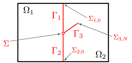
Figure 1: Example of a 2D domain with 3 intersecting fractures $\Gamma_{1},\Gamma_{2},\Gamma_{3}$ and 2 connected components $\Omega_{1}$, $\Omega_{2}$.

We will denote by $d\tau({\bf x})$ the $d-1$ dimensional Lebesgue measure on $\Gamma$. On the fracture network ${\Gamma}$, we define the function space $L^{2}(\Gamma)=\{v=(v_{i})_{i\in I},v_{i}\in L^{2}(\Gamma_{i}),i\in I\},$ endowed with the norm $\|v\|^{2}_{L^{2}(\Gamma)}=\sum_{i\in I}\|v_{i}\|^{2}_{L^{2}(\Gamma_{i})}$. Its subspace $H^{1}(\Gamma)$ is defined as the space of functions $v=(v_{i})_{i\in I}$ such that $v_{i}\in H^{1}(\Gamma_{i})$, $i\in I$ with continuous traces at the fracture intersections. The space $H^{1}(\Gamma)$ is endowed with the norm $\|v\|^{2}_{H^{1}(\Gamma)}=\sum_{i\in I}\|v_{i}\|^{2}_{H^{1}(\Gamma_{i})}$ and its subspace with vanishing traces on $\Sigma_{0}=\bigcup_{i\in I}\Sigma_{i,0}$ is denoted by $H^{1}_{\Sigma_{0}}(\Gamma)$.

Let us also consider the trace operator $\gamma_{i}$ from $H^{1}(\Omega)$ to $L^{2}(\Gamma_{i})$ as well as the trace operator $\gamma$ from $H^{1}(\Omega)$ to $L^{2}(\Gamma)$ such that $(\gamma v)_{i}=\gamma_{i}(v)$ for all $i\in I$.

On $\Omega$, the gradient operator from $H^{1}(\Omega)$ to $L^{2}(\Omega)^{d}$ is denoted by $\nabla$. On the fracture network ${\Gamma}$, the tangential gradient $\nabla_{\tau}$ acting from $H^{1}(\Gamma)$ to $L^{2}(\Gamma)^{d-1}$ is defined by

$$\nabla_{\tau}v=(\nabla_{\tau_{i}}v_{i})_{i\in I},$$

where, for each $i\in I$, the tangential gradient $\nabla_{\tau_{i}}$ is defined from $H^{1}({\Gamma}_{i})$ to $L^{2}({\Gamma}_{i})^{d-1}$ by fixing a reference Cartesian coordinate system of the plane ${\cal P}_{i}$ containing ${\Gamma}_{i}$. We also denote by ${\mbox{\rm div}}_{\tau_{i}}$ the divergence operator from $H_{{\mbox{\rm div}}}(\Gamma_{i})$ to $L^{2}(\Gamma_{i})$.

The function spaces arising in the variational formulation of the hybrid dimensional Darcy flow model are

$$V=\{v\in H^{1}(\Omega)\mbox{ such that }\gamma v\in H^{1}(\Gamma)\},$$

and its subspace

$$V^{0}=\{v\in H^{1}_{0}(\Omega)\mbox{ such that }\gamma v\in H^{1}_{\Sigma_{0}}(\Gamma)\}.$$

The space $V^{0}$ is endowed with the following Hilbertian norm

$$\|v\|_{V^{0}}=\Bigl{(}\|\nabla v\|^{2}_{L^{2}(\Omega)^{d}}+\|\nabla_{\tau}\gamma v\|^{2}_{L^{2}(\Gamma)^{d-1}}\Bigr{)}^{1/2}.$$

Let $\Omega_{\alpha},\alpha\in{\cal A}$ denote the connected components of $\Omega\setminus\overline{\Gamma}$, with ${\cal A}$ being the set of connected components of $\Omega\setminus\overline{\Gamma}$. Let us define the space $H_{{\mbox{\rm div}}}(\Omega\setminus\overline{\Gamma})=\{{\bf q}_{m}=({\bf q}_{m,\alpha})_{\alpha\in{\cal A}}\,|\,{\bf q}_{m,\alpha}\in H_{{\mbox{\rm div}}}(\Omega_{\alpha})\}$. Using the orientation of ${\cal P}_{i}$ we can define the two sides $\pm$ of the fracture $\Gamma_{i}$, for all $i\in I$. For all ${\bf q}_{m}\in H_{{\mbox{\rm div}}}(\Omega\setminus\overline{\Gamma})$, let $\gamma_{{\bf n},i}^{\pm}{\bf q}_{m}$ denote the normal trace of ${\bf q}_{m}$ on the side $\pm$ of $\Gamma_{i}$ with the normal oriented outward from the side $\pm$. Let us define the Hilbert function space

$$\left.\begin{array}[]{r@{\,\,}c@{\,\,}l}H(\Omega,\Gamma)=\displaystyle\{&&{\bf q}_{m}=({\bf q}_{m,\alpha})_{\alpha\in{\cal A}},\,{\bf q}_{f}=({\bf q}_{f,i})_{i\in I}\,|\,{\bf q}_{m}\in H_{{\mbox{\rm div}}}(\Omega\setminus\overline{\Gamma}),\\ &&\displaystyle{\bf q}_{f,i}\in L^{2}(\Gamma_{i})^{d-1},\,{\mbox{\rm div}}_{\tau_{i}}({\bf q}_{f,i})-\gamma_{{\bf n},i}^{+}{\bf q}_{m}-\gamma_{{\bf n},i}^{-}{\bf q}_{m}\in L^{2}(\Gamma_{i}),i\in I\},\end{array}\right.$$

and its closed Hilbert subspace

$$\left.\begin{array}[]{r@{\,\,}c@{\,\,}l}&&W(\Omega,\Gamma)=\displaystyle\{({\bf q}_{m},{\bf q}_{f})\in H(\Omega,\Gamma)\,|\,\displaystyle\sum_{\alpha\in{\cal A}}\int_{\Omega_{\alpha}}({\bf q}_{m,\alpha}\cdot\nabla v+{\mbox{\rm div}}({\bf q}_{m,\alpha})v)d{\bf x}\\ &&\displaystyle+\sum_{i\in I}\int_{\Gamma_{i}}({\bf q}_{f,i}\cdot\nabla_{\tau_{i}}\gamma_{i}v+({\mbox{\rm div}}_{\tau_{i}}({\bf q}_{f,i})-\gamma_{{\bf n},i}^{+}{\bf q}_{m}-\gamma_{{\bf n},i}^{-}{\bf q}_{m})\gamma_{i}v)d\tau({\bf x})=0\,\forall\,v\in V^{0}\}.\end{array}\right.$$ (3)

The last definition corresponds to imposing in a weak sense the conditions $\sum_{i\in I}\gamma_{{\bf n},\Sigma_{i}}{\bf q}_{f,i}=0$ on $\Sigma\setminus\Sigma_{0}$ and $\gamma_{{\bf n},\Sigma_{i}}{\bf q}_{f,i}=0$ on $\Sigma_{i,N},i\in I$, where $\gamma_{{\bf n},\Sigma_{i}}$ is the normal trace operator on $\Sigma_{i}$ (tangent to $\Gamma_{i}$) with the normal oriented outward from $\Gamma_{i}$, and using the extension of $\gamma_{{\bf n},\Sigma_{i}}{\bf q}_{f,i}$ by zero on $\Sigma\setminus\Sigma_{i}$.

2.2 Hybrid dimensional Darcy Flow Model

In the matrix domain $\Omega\setminus\overline{\Gamma}$ (resp. in the fracture network ${\Gamma}$), let us denote by $\Lambda_{m}\in L^{\infty}(\Omega)^{d\times d}$ (resp. $\Lambda_{f}\in L^{\infty}(\Gamma)^{(d-1)\times(d-1)}$) the permeability tensor such that there exist $\overline{\lambda}_{m}\geq\underline{\lambda}_{m}>0$ (resp. $\overline{\lambda}_{f}\geq\underline{\lambda}_{f}>0$) with

$$\underline{\lambda}_{m}|\boldsymbol{\xi}|^{2}\leq(\Lambda_{m}({\bf x})\boldsymbol{\xi},\boldsymbol{\xi})\leq\overline{\lambda}_{m}|\boldsymbol{\xi}|^{2}\mbox{ for all }\boldsymbol{\xi}\in\mathbb{R}^{d},{\bf x}\in\Omega,$$

(resp. $\underline{\lambda}_{f}|\boldsymbol{\xi}|^{2}\leq(\Lambda_{f}({\bf x})\boldsymbol{\xi},\boldsymbol{\xi})\leq\overline{\lambda}_{f}|\boldsymbol{\xi}|^{2}\mbox{ for all }\boldsymbol{\xi}\in\mathbb{R}^{d-1},{\bf x}\in\Gamma$).

We also denote by $\mu$ the fluid viscosity which is assumed constant and by $d_{f}\in L^{\infty}({\Gamma})$ the width of the fractures assumed to be such that there exist ${\overline{d}}_{f}\geq{\underline{d}}_{f}>0$ with ${\underline{d}}_{f}\leq d_{f}({\bf x})\leq{\overline{d}}_{f}$ for all ${\bf x}\in\Gamma$.

Given $\bar{u}\in V$, the strong formulation of the hybrid dimensional Darcy flow model amounts to: find $u\in V$ and $({\bf q}_{m},{\bf q}_{f})\in W(\Omega,\Gamma)$ such that $u-\bar{u}\in V^{0}$ and

$$\left\{\begin{array}[]{r@{\,\,}c@{\,\,}ll}{\mbox{\rm div}}({\bf q}_{m,\alpha})&=&0&\mbox{ on }\Omega_{\alpha},\alpha\in{\cal A},\\ {\bf q}_{m,\alpha}&=&-{\Lambda_{m}\over\mu}\nabla u&\mbox{ on }\Omega_{\alpha},\alpha\in{\cal A},\\ {\mbox{\rm div}}_{\tau_{i}}({\bf q}_{f,i})-\gamma_{{\bf n},i}^{+}{\bf q}_{m}-\gamma_{{\bf n},i}^{-}{\bf q}_{m}&=&0&\mbox{ on }{\Gamma}_{i},i\in I,\\ {\bf q}_{f,i}&=&-d_{f}~{}{\Lambda_{f}\over\mu}\nabla_{\tau_{i}}\gamma_{i}u&\mbox{ on }{\Gamma}_{i},i\in I.\end{array}\right.$$ (8)

The weak formulation of (8) amounts to: find $u\in V$ such that $u-\bar{u}\in V^{0}$ and the following variational equation is satisfied for all $v\in V^{0}$:

$$\displaystyle\int_{\Omega}{\Lambda_{m}({\bf x})\over\mu}\nabla u({\bf x})\cdot\nabla v({\bf x})d{\bf x}+\displaystyle\int_{\Gamma}d_{f}({\bf x}){\Lambda_{f}({\bf x})\over\mu}\nabla_{\tau}\gamma u({\bf x})\cdot\nabla_{\tau}\gamma v({\bf x})d\tau({\bf x})=0.$$ (9)

The existence and uniqueness of the solution to (9) derives from the Lax Milgram theorem and a Poincaré inequality stated in [12].

2.3 Hybrid dimensional transport model

Let $\gamma_{\bf n}$ be the normal trace operator on $\partial\Omega$ with the normal oriented outward from $\Omega$. Let us define $\partial\Omega^{-}=\{{\bf x}\in\partial\Omega\,|\,\gamma_{\bf n}{\bf q}_{m}({\bf x})<0\}$, $\Sigma_{i,0}^{-}=\{{\bf x}\in\Sigma_{i,0}\,|\,\gamma_{{\bf n},\Sigma_{i}}{\bf q}_{f,i}({\bf x})<0\}$, $i\in I$, as well as the following subset of $\Sigma\setminus\Sigma_{0}$:

$$\Sigma^{-}=\{{\bf x}\in\Sigma\setminus\Sigma_{0}\,|\,\sum_{i\in I}|\gamma_{{\bf n},\Sigma_{i}}{\bf q}_{f,i}({\bf x})|\neq 0\}.$$

We consider a linear, purely advective model with velocity ${\bf q}_{m}$ in the matrix domain and ${\bf q}_{f}$ in the fracture network. The matrix concentration is denoted by $c_{m}$ ($c_{m,\alpha}$ in each connected component $\Omega_{\alpha}$, $\alpha\in{\cal A}$) and the fracture concentration, representing the average concentration in the fracture width, is denoted by $c_{f}$ ($c_{f,i}$ in each fracture $\Gamma_{i}$, $i\in I$). The 2D equation in the fracture network is as usual obtained by integration of the 3D advection equation in the width of the fractures. For a purely advective equation, the transmission condition at the matrix fracture interfaces states that the input normal flux in the matrix is obtained using the upwind fracture concentration $c_{f}$. At the fracture intersection $\Sigma^{-}$, an additional unknown $c_{f,\Sigma^{-}}$ must be introduced and the transmission conditions state that the normal fluxes sum to zero and that the input normal fluxes are obtained using the upwind concentration $c_{f,\Sigma^{-}}$.

Let be given the input boundary conditions $\bar{c}_{m}\in L^{\infty}(\partial\Omega^{-})$, $\bar{c}_{f,i}\in L^{\infty}(\Sigma_{i,0}^{-})$, $i\in I$, and the initial conditions $c_{m}^{0}\in L^{\infty}(\Omega\setminus\overline{\Gamma})$, $c_{f}^{0}\in L^{\infty}({\Gamma})$. Let us denote by $\phi_{m}({\bf x})$ the porosity in the matrix and by $\phi_{f}({\bf x})$ the porosity in the fracture network. The transport hybrid dimensional model amounts to: find $c_{m}\in L^{\infty}\Bigl{(}(\Omega\setminus\overline{\Gamma})\times(0,T)\Bigr{)}$, $c_{f}\in L^{\infty}\Bigl{(}{\Gamma}\times(0,T)\Bigr{)}$, and $c_{f,\Sigma^{-}}\in L^{\infty}\Bigl{(}\Sigma^{-}\times(0,T)\Bigr{)}$, such that:

$$\left\{\begin{array}[]{r@{\,\,}c@{\,\,}ll}\phi_{m}\partial_{t}c_{m,\alpha}+{\mbox{\rm div}}(c_{m,\alpha}{\bf q}_{m,\alpha})&=&0&\mbox{ on }\Omega_{\alpha}\times(0,T),\alpha\in{\cal A}\\ \phi_{f}d_{f}\partial_{t}c_{f,i}+{\mbox{\rm div}}_{\tau_{i}}(c_{f,i}{\bf q}_{f,i})&=&\gamma_{{\bf n},i}^{+}c_{m}{\bf q}_{m}+\gamma_{{\bf n},i}^{-}c_{m}{\bf q}_{m}&\mbox{ on }{\Gamma}_{i}\times(0,T),i\in I,\\ (\gamma_{{\bf n},i}^{\pm}c_{m}{\bf q}_{m})^{-}&=&c_{f}(\gamma_{{\bf n},i}^{\pm}{\bf q}_{m})^{-}&\mbox{ on }{\Gamma}_{i}\times(0,T),i\in I,\\ (\gamma_{{\bf n},\Sigma_{i}}c_{f,i}{\bf q}_{f,i})^{-}&=&c_{f,\Sigma^{-}}(\gamma_{{\bf n},\Sigma_{i}}{\bf q}_{f,i})^{-}&\mbox{ on }(\Sigma_{i}\setminus\Sigma_{i,0})\times(0,T),i\in I,\\ \displaystyle\sum_{j\in I}\gamma_{{\bf n},\Sigma_{j}}c_{f,j}{\bf q}_{f,j}&=&0&\mbox{ on }(\Sigma\setminus\Sigma_{0})\times(0,T),\\ (\gamma_{\bf n}c_{m}{\bf q}_{m})^{-}&=&\bar{c}_{m}(\gamma_{\bf n}q_{m})^{-}&\mbox{ on }\partial\Omega\times(0,T),\\ (\gamma_{{\bf n},\Sigma_{i}}c_{f,i}{\bf q}_{f,i})^{-}&=&\bar{c}_{f,i}(\gamma_{{\bf n},\Sigma_{i}}{\bf q}_{f,i})^{-}&\mbox{ on }\Sigma_{i,0}\times(0,T),i\in I,\\ c_{m}&=&c_{m}^{0}&\mbox{ on }(\Omega\setminus\overline{\Gamma})\times\{t=0\},\\ c_{f}&=&c_{f}^{0}&\mbox{ on }{\Gamma}\times\{t=0\},\end{array}\right.$$ (19)

where the notations $a^{+}=\max(a,0)$ and $a^{-}=\min(a,0)$ are used for all $a\in\mathbb{R}$.

3 Vertex Approximate Gradient Discretization (VAG)

3.1 VAG discretization of the Darcy flow model

In the spirit of [19], we consider generalized polyhedral meshes of $\Omega$ in the sense that the edges of the mesh are linear but its faces are not necessarily planar. Roughly speaking, each face is assumed to be defined by the union of the triangles joining each edge of the face to a so called face centre. This definition has the advantage to include in particular hexahedral cells with non planar faces.

Let ${\cal M}$ be the set of cells which are disjoint open polyhedral subsets of $\Omega$ such that $\bigcup_{K\in{\cal M}}\overline{K}=\overline{\Omega}$. For each $K\in{\cal M}$, it is assumed that there exists ${{\bf x}}_{K}\in K\setminus\partial K$, the so-called “centre” of the cell $K$, such that $K$ is star-shaped with respect to ${{\bf x}}_{K}$. We then denote by ${\cal F}_{K}$ the set of interfaces of non zero $d-1$ dimensional measure among the interior faces $\overline{K}\cap\overline{L}$, $L\in{\cal M}\setminus\{K\}$, and the boundary interface $\overline{K}\cap\partial\Omega$, which possibly splits in several boundary faces. Let us denote by

$${\cal F}=\bigcup_{K\in{\cal M}}{\cal F}_{K}$$

the set of all faces of the mesh. Note that the faces are not assumed to be planar, hence the term “generalized polyhedral mesh”. For $\sigma\in{\cal F}$, let ${\cal E}_{\sigma}$ be the set of interfaces of non zero, $d-2$ dimensional measure among the interfaces $\overline{\sigma}\cap\overline{\sigma}^{\prime}$, $\sigma^{\prime}\in{{\cal F}}\setminus\{\sigma\}$. Then, we denote by

$${\cal E}=\bigcup_{\sigma\in{\cal F}}{\cal E}_{\sigma}$$

the set of all edges of the mesh. Let ${\cal V}_{\sigma}=\bigcup_{\left(e,e^{\prime}\right)\in{\cal E}^{2}_{\sigma},e\neq e^{\prime}}\big{(}e\cap e^{\prime}\big{)}$ be the set of nodes of $\sigma$. For each $K\in{\cal M}$ we define ${\cal V}_{K}=\bigcup_{\sigma\in{\cal F}_{K}}{\cal V}_{\sigma},$ and we also denote by

$${\cal V}=\bigcup_{K\in{\cal M}}{\cal V}_{K}$$

the set of all nodes of the mesh. It is then assumed that for each face $\sigma\in{\cal F}$, there exists a so-called “centre” of the face ${{\bf x}}_{\sigma}\in{\sigma}\setminus\bigcup_{e\in{\cal E}_{\sigma}}e$ such that ${{\bf x}}_{\sigma}=\sum_{{\bf s}\in{\cal V}_{\sigma}}\beta_{\sigma,{\bf s}}~{}{\bf x}_{\bf s},\mbox{ with }\sum_{{\bf s}\in{\cal V}_{\sigma}}\beta_{\sigma,{\bf s}}=1,$ and $\beta_{\sigma,{\bf s}}\geq 0$ for all ${\bf s}\in{\cal V}_{\sigma}$; moreover the face $\sigma$ is assumed to be defined by the union of the triangles $T_{\sigma,e}$ defined by the face centre ${{\bf x}}_{\sigma}$ and each edge $e\in{\cal E}_{\sigma}$.

The mesh is also supposed to be conforming w.r.t. the fracture network ${\Gamma}$ in the sense that for each $i\in I$ there exists a subset ${\cal F}_{{\Gamma}_{i}}$ of ${\cal F}$ such that $\overline{\Gamma}_{i}=\bigcup_{\sigma\in{\cal F}_{{\Gamma}_{i}}}\overline{\sigma}.$ We will denote by ${\cal F}_{\Gamma}$ the set of fracture faces $\bigcup_{i\in I}{\cal F}_{{\Gamma}_{i}}$. The following notations will be used for convenience:

$${\cal M}_{\bf s}=\{K\in{\cal M}\,|\,{\bf s}\in{\cal V}_{K}\},$$

$${\cal M}_{\sigma}=\{K\in{\cal M}\,|\,\sigma\in{\cal F}_{K}\},$$

$${\cal F}_{{\Gamma},{\bf s}}=\{\sigma\in{\cal F}_{\Gamma}\,|\,{\bf s}\in{\cal V}_{\sigma}\},$$

and

$${\cal F}_{\Gamma,K}={\cal F}_{K}\cap{{\cal F}_{\Gamma}}.$$

This geometrical discretization of $\Omega$ and ${\Gamma}$ is denoted in the following by ${\cal D}$.

The VAG discretization was introduced in [19] for diffusive problems on heterogeneous, anisotropic media. Its extension to the hybrid dimensional Darcy model is based on the following vector space of unknowns:

$$X_{\cal D}=\{v_{K},v_{\bf s},v_{\sigma}\in\mathbb{R},K\in{\cal M},{\bf s}\in{\cal V},\sigma\in{\cal F}_{\Gamma}\},$$

and its subspace with homogeneous Dirichlet boundary conditions on $\partial\Omega$:

$$X_{\cal D}^{0}=\{v\in X_{\cal D}\,|\,v_{\bf s}=0\mbox{ for }{\bf s}\in{\cal V}_{ext}\}.$$

where ${\cal V}_{ext}={\cal V}\cap\partial\Omega$ denotes the set of boundary nodes, and ${\cal V}_{int}={\cal V}\setminus\partial\Omega$ denotes the set of interior nodes.

A finite element discretization of $V$ is built using a tetrahedral sub-mesh of ${\cal M}$ and a second order interpolation at the face centres ${\bf x}_{\sigma}$, $\sigma\in{\cal F}\setminus{\cal F}_{\Gamma}$ defined by the operator $I_{\sigma}:X_{\cal D}\rightarrow\mathbb{R}$ such that

$$I_{\sigma}(v)=\sum_{{\bf s}\in{\cal V}_{\sigma}}\beta_{\sigma,{\bf s}}v_{\bf s}.$$

The tetrahedral sub-mesh is defined by ${\cal T}=\{T_{K,\sigma,e},e\in{\cal E}_{\sigma},\sigma\in{\cal F}_{K},K\in{\cal M}\}$ where $T_{K,\sigma,e}$ is the tetrahedron joining the cell centre ${{\bf x}}_{K}$ to the triangle $T_{\sigma,e}$ (see Figure 2 for examples of such tetrahedra).

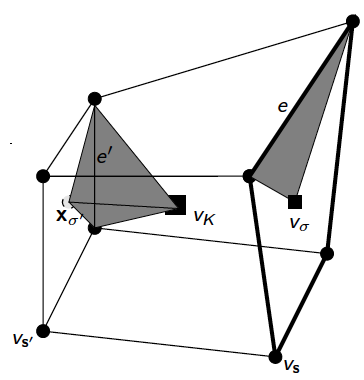
Figure 2: For a cell $K$ with one fracture face $\sigma$ in bold: cell unknown $v_{K}$ located at ${\bf x}_{K}$, fracture-face unknown $v_{\sigma}$ located at ${\bf x}_{\sigma}$, node unknowns $v_{\bf s},v_{{\bf s}^{\prime}}$, face centre ${\bf x}_{\sigma^{\prime}}$ of face $\sigma^{\prime}$, triangle $T_{\sigma,e}$ (convex hull of $e$ and ${\bf x}_{\sigma}$), triangle $T_{\sigma^{\prime},e^{\prime}}$ (convex hull of $e^{\prime}$ and ${\bf x}_{\sigma^{\prime}}$) and tetrahedron $T_{K,\sigma^{\prime},e^{\prime}}$ (convex hull of ${\bf x}_{K}$, ${\bf x}_{\sigma^{\prime}}$ and $e^{\prime}$).

For a given $v\in X_{\cal D}$, we define the function $\pi_{\cal T}v\in V$ as the continuous piecewise affine function on each tetrahedron of ${\cal T}$ such that $\pi_{\cal T}v({{\bf x}}_{K})=v_{K}$, $\pi_{\cal T}v({\bf s})=v_{\bf s}$, $\pi_{\cal T}v({{\bf x}}_{\sigma})=v_{\sigma}$, and $\pi_{\cal T}v({{\bf x}}_{\sigma^{\prime}})=I_{\sigma^{\prime}}(v)$ for all $K\in{\cal M}$, ${\bf s}\in{\cal V}$, $\sigma\in{\cal F}_{\Gamma}$, and $\sigma^{\prime}\in{\cal F}\setminus{\cal F}_{\Gamma}$. The nodal basis of this finite element discretization will be denoted by $\eta_{K}$, $\eta_{\bf s}$, $\eta_{\sigma}$, for $K\in{\cal M}$, ${\bf s}\in{\cal V}$, $\sigma\in{\cal F}_{\Gamma}$.

The VAG discretization of the hybrid dimensional Darcy flow model (8) is based on its weak formulation (9). Given $\bar{u}_{\bf s},{\bf s}\in{\cal V}_{ext}$, it amounts to: find $u_{\cal D}\in X_{\cal D}$ with $u_{\bf s}=\bar{u}_{\bf s}$ for all ${\bf s}\in{\cal V}_{ext}$ and such that for all $v_{\cal D}\in X_{\cal D}^{0}$ one has

$$\int_{\Omega}{\Lambda_{m}({\bf x})\over\mu}\nabla\pi_{\cal T}u_{\cal D}({\bf x})\cdot\nabla\pi_{\cal T}v_{\cal D}({\bf x})d{\bf x}+\int_{\Gamma}d_{f}({\bf x}){\Lambda_{f}({\bf x})\over\mu}\nabla_{\tau}\gamma\pi_{\cal T}u_{\cal D}({\bf x})\cdot\nabla_{\tau}\gamma\pi_{\cal T}v_{\cal D}({\bf x})d\tau({\bf x})=0.$$ (20)

Following [12], this Galerkin Finite Element formulation (20) can be reformulated in terms of discrete conservation laws using the following definition of the VAG fluxes. For all $v_{\cal D}\in X_{\cal D}$, the VAG matrix fluxes connect the cell $K\in{\cal M}$ to its nodes and fracture faces $\nu\in{\cal V}_{K}\cup{\cal F}_{\Gamma,K}$:

$$F_{K,\nu}(v_{\cal D})=-\int_{K}{\Lambda_{m}({\bf x})\over\mu}\nabla\pi_{\cal T}v_{\cal D}({\bf x})\cdot\nabla\eta_{\nu}({\bf x})d{\bf x}=\sum_{\nu^{\prime}\in{\cal V}_{K}\cup{\cal F}_{\Gamma,K}}a_{K,\nu}^{\nu^{\prime}}(v_{K}-v_{\nu^{\prime}})$$ (21)

with $a_{K,\nu}^{\nu^{\prime}}=\int_{K}{\Lambda_{m}({{\bf x}})\over\mu}\nabla\eta_{\nu}({{\bf x}})\cdot\nabla\eta_{\nu^{\prime}}({{\bf x}})d{\bf x}.$ The VAG fracture fluxes connect the face $\sigma\in{{\cal F}_{\Gamma}}$ to its nodes ${\bf s}\in{\cal V}_{\sigma}$:

$$F_{\sigma,{\bf s}}(v_{\cal D})=-\int_{\sigma}d_{f}({\bf x}){\Lambda_{f}({\bf x})\over\mu}\nabla_{\tau}\gamma\pi_{\cal T}v_{\cal D}({\bf x})\cdot\nabla_{\tau}\gamma\eta_{\bf s}({\bf x})d\tau({\bf x})=\sum_{{\bf s}^{\prime}\in{\cal V}_{\sigma}}a_{\sigma,{\bf s}}^{{\bf s}^{\prime}}(v_{\sigma}-v_{{\bf s}^{\prime}})$$ (22)

with $a_{\sigma,{\bf s}}^{{\bf s}^{\prime}}=\int_{\sigma}d_{f}({\bf x}){\Lambda_{f}({{\bf x}})\over\mu}\nabla_{\tau}\gamma\eta_{\bf s}({{\bf x}})\cdot\nabla_{\tau}\gamma\eta_{{\bf s}^{\prime}}({{\bf x}})d\tau({\bf x}).$

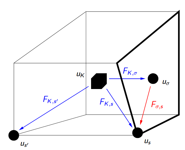
Figure 3: Matrix fluxes (in blue) and fracture fluxes (in red) inside a cell $K$ with a fracture face $\sigma$ (in bold). The matrix fluxes $F_{K,\nu}$ connect the cell $K$ to its nodes and fracture faces $\nu\in{\cal V}_{K}\cup{\cal F}_{\Gamma,K}$. The fracture fluxes $F_{\sigma,{\bf s}}$ connect the face $\sigma$ to the nodes ${\bf s}\in{\cal V}_{\sigma}$ of $\sigma$.

Then, the Galerkin Finite Element formulation (20) is equivalent to: find $u_{\cal D}\in X_{\cal D}$ satisfying the following set of discrete conservation equations and Dirichlet boundary conditions:

$$\left\{\begin{array}[]{r@{\,\,}c@{\,\,}ll}&&\displaystyle\sum_{{\bf s}\in{\cal V}_{K}}F_{K,{\bf s}}(u_{\cal D})+\sum_{\sigma\in{\cal F}_{\Gamma,K}}F_{K,\sigma}(u_{\cal D})=0,\,\,K\in{\cal M}\\ &&\displaystyle\sum_{{\bf s}\in{{\cal V}}_{\sigma}}F_{\sigma,{\bf s}}(u_{\cal D})+\sum_{K\in{\cal M}_{\sigma}}-F_{K,\sigma}(u_{\cal D})=0,\,\,\sigma\in{{\cal F}}_{\Gamma}\\ &&\displaystyle\sum_{K\in{\cal M}_{\bf s}}-F_{K,{\bf s}}(u_{\cal D})+\sum_{\sigma\in{\cal F}_{\Gamma,{\bf s}}}-F_{\sigma,{\bf s}}(u_{\cal D})=0,\,\,{\bf s}\in{\cal V}_{int},\\ &&u_{\bf s}=\bar{u}_{\bf s},\,\,{\bf s}\in{\cal V}_{ext}.\end{array}\right.$$

3.2 First order upwind discretization of the transport model

3.2.1 Definition of control volumes

The VAG discretization of the hybrid dimensional transport model combines the VAG matrix and fracture fluxes (21), (22) with the following definition of the control volumes based on partitions of the cells and of the fracture faces. These partitions are respectively denoted, for all $K\in{\cal M}$, by

$$\overline{K}~{}=~{}\overline{\omega}_{K}~{}\cup~{}\Bigl{(}\bigcup_{{\bf s}\in{\cal V}_{K}\setminus({\cal V}_{ext}\cup{\cal V}_{\Gamma})}\overline{\omega}_{K,{\bf s}}\Bigr{)}$$

and, for all $\sigma\in{\cal F}_{\Gamma}$, by

$$\overline{\sigma}~{}=~{}\overline{\omega}_{\sigma}~{}\cup~{}\Bigl{(}\bigcup_{{\bf s}\in{\cal V}_{\sigma}\setminus{\cal V}_{ext}}\overline{\omega}_{\sigma,{\bf s}}\Bigr{)}.$$

Then, the control volumes are defined by $\omega_{K}$ for all cells $K\in{\cal M}$, by $\omega_{\sigma}$ for all fracture faces $\sigma\in{\cal F}_{\Gamma}$, and by

$$\overline{\omega}_{\bf s}=\bigcup_{K\in{\cal M}_{\bf s}}\overline{\omega}_{K,{\bf s}},$$

for all nodes ${\bf s}\in{\cal V}_{int}\setminus{\cal V}_{\Gamma}$, and by

$$\overline{\omega}_{\bf s}=\bigcup_{\sigma\in{\cal F}_{\Gamma,{\bf s}}}\overline{\omega}_{\sigma,{\bf s}},$$

for all nodes ${\bf s}\in{\cal V}_{\Gamma}\setminus{\cal V}_{ext}$. Note that this definition avoid the mixing of the fracture and matrix rocktypes at the control volumes ${\bf s}\in{\cal V}_{\Gamma}\setminus{\cal V}_{ext}$ and $\sigma\in{\cal F}_{\Gamma}$. This is exhibited in Figure 4 in comparison with an alternative choice mixing the matrix and fracture rocktypes which artificially enlarges the fractures. We refer to [12] for numerical comparisons on a two phase flow model of these two types of choices of the control volumes.

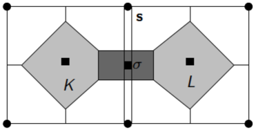
Figure 4: Example of choices of the control volumes at cells, fracture face, and nodes, in the case of two cells $K$ and $L$ splitted by one fracture face $\sigma$ (the width of the fracture has been enlarged in this figure). The left figure exhibits the good choice with no mixing of fracture and matrix rocktypes while the right figure exhibits the bad choice enlarging artificially the fracture.

The same idea is applied for all nodes located at different rocktype interfaces. In practice, for such a node ${\bf s}\in{\cal V}_{int}\setminus{\cal V}_{\Gamma}$ (resp. ${\bf s}\in{\cal V}_{\Gamma}\setminus{\cal V}_{ext}$), the set $\omega_{K,{\bf s}}$ (resp. $\omega_{\sigma,{\bf s}}$) should be non empty only for the cell(s) $K$ (resp. fracture face(s) $\sigma$) with the largest permeability among those around the node ${\bf s}$ (see [20] for details).

In practice, the above partitions of the cells and fracture faces does not need to be built. It is sufficient to define the matrix volume fractions

$$\alpha_{K,{\bf s}}={\int_{\omega_{K,{\bf s}}}d{\bf x}\over\int_{K}d{\bf x}},{\bf s}\in{\cal V}_{K}\setminus({\cal V}_{ext}\cup{\cal V}_{\Gamma}),K\in{\cal M},$$

constrained to satisfy $\alpha_{K,{\bf s}}\geq 0$, and $\sum_{{\bf s}\in{\cal V}_{K}\setminus({\cal V}_{ext}\cup{\cal V}_{\Gamma})}\alpha_{K,{\bf s}}\leq 1$, as well as the fracture volume fractions

$$\alpha_{\sigma,{\bf s}}={\int_{\omega_{\sigma,{\bf s}}}d_{f}({\bf x})d\tau({\bf x})\over\int_{\sigma}d_{f}({\bf x})d\tau({\bf x})},{\bf s}\in{\cal V}_{\sigma}\setminus{\cal V}_{ext},\sigma\in{\cal F}_{\Gamma},$$

such that $\alpha_{\sigma,{\bf s}}\geq 0$, and $\sum_{{\bf s}\in{\cal V}_{\sigma}\setminus{\cal V}_{ext}}\alpha_{\sigma,{\bf s}}\leq 1$. Then, the porous volumes of the control volumes are set to

$$\phi_{K}=(1-\sum_{{\bf s}\in{\cal V}_{K}\setminus({\cal V}_{\Gamma}\cup{\cal V}_{ext})}\alpha_{K,s})\int_{K}\phi_{m}({\bf x})d{\bf x},\,\,K\in{\cal M}$$

$$\phi_{\sigma}=(1-\sum_{{\bf s}\in{{\cal V}}_{\sigma}\setminus{\cal V}_{ext}}\alpha_{\sigma,{\bf s}})d_{f,\sigma}\int_{\sigma}\phi_{f}({\bf x})d\tau({\bf x}),\,\,\sigma\in{\cal F}_{\Gamma},$$

$$\phi_{\bf s}=\sum_{\sigma\in{\cal F}_{\Gamma,{\bf s}}}\alpha_{\sigma,{\bf s}}d_{f,\sigma}\int_{\sigma}\phi_{f}({\bf x})d\tau({\bf x}),\,\,{\bf s}\in{\cal V}_{\Gamma}\setminus{\cal V}_{ext},$$

$$\phi_{\bf s}=\sum_{K\in{\cal M}_{{\bf s}}}\alpha_{K,{\bf s}}\int_{K}\phi_{m}({\bf x})d{\bf x},\,\,{\bf s}\in{\cal V}\setminus({\cal V}_{ext}\cup{\cal V}_{\Gamma}),$$

with $d_{f,\sigma}=\displaystyle{\int_{\sigma}d_{f}({\bf x})d\tau({\bf x})\over\int_{\sigma}d\tau({\bf x})}$.

3.2.2 Time integration

For $N\in\mathbb{N}^{*}$, let us consider the time discretization $t^{0}=0<t^{1}<\cdots<t^{n-1}<t^{n}\cdots<t^{N}=T$ of the time interval $[0,T]$. We denote the time steps by $\Delta t^{n}=t^{n+1}-t^{n}$ for all $n=0,\cdots,N-1$.

Given $\bar{c}_{\bf s},{\bf s}\in{\cal V}_{ext}$ with arbitrary values on the set of ouput boundary nodes

$${\cal V}_{ext}^{+}=\{{\bf s}\in{\cal V}_{ext}\,|\,F_{K,{\bf s}}(u_{\cal D})\geq 0\,\forall K\in{\cal M}_{\bf s}\mbox{ and }F_{\sigma,{\bf s}}(u_{\cal D})\geq 0\,\forall\sigma\in{\cal F}_{{\Gamma},{\bf s}}\},$$

and $c_{\cal D}^{0}\in X_{\cal D}$ such that $c_{\bf s}^{0}=\bar{c}_{\bf s}$ for all ${\bf s}\in{\cal V}_{ext}$, the transport discrete model amounts to find $c_{\cal D}^{n+1}\in X_{\cal D}$ for all $n=0,\cdots,N-1$ satisfying the following discrete conservation laws and Dirichlet input conditions

$$\left\{\begin{array}[]{r@{\,\,}c@{\,\,}ll}&&\displaystyle\phi_{K}{c_{K}^{n+1}-c_{K}^{n}\over\Delta t^{n}}+\sum_{{\bf s}\in{{\cal V}}_{K}}H_{K,{\bf s}}(c_{\cal D}^{n})+\sum_{\sigma\in{{\cal F}}_{\Gamma,K}}H_{K,\sigma}(c_{\cal D}^{n})=0,\,\,K\in{\cal M},\\ &&\displaystyle\phi_{\sigma}{c_{\sigma}^{n+1}-c_{\sigma}^{n}\over\Delta t^{n}}+\sum_{{\bf s}\in{{\cal V}}_{\sigma}}H_{\sigma,{\bf s}}(c_{\cal D}^{n})-\sum_{K\in{\cal M}_{\sigma}}H_{K,\sigma}(c_{\cal D}^{n})=0,\,\,\sigma\in{{\cal F}}_{\Gamma},\\ &&\displaystyle\phi_{\bf s}{c_{{\bf s}}^{n+1}-c_{{\bf s}}^{n}\over\Delta t^{n}}-\sum_{K\in{\cal M}_{\bf s}}H_{K,{\bf s}}(c_{\cal D}^{n})-\sum_{\sigma\in{\cal F}_{\Gamma,{\bf s}}}H_{\sigma,{\bf s}}(c_{\cal D}^{n})=0,\,\,{\bf s}\in{\cal V}_{int},\\ &&c_{\bf s}^{n+1}=\bar{c}_{\bf s},\,\,{\bf s}\in{\cal V}_{ext},\end{array}\right.$$

with the following explicit upwind two point fluxes

$$\begin{array}[]{l}H_{K,\nu}(c^{n}_{\cal D})=c_{K}^{n}F_{K,\nu}(u_{\cal D})^{+}+c_{\nu}^{n}F_{K,\nu}(u_{\cal D})^{-}\\ \\ H_{\sigma,{\bf s}}(c^{n}_{\cal D})=c_{\sigma}^{n}F_{\sigma,{\bf s}}(u_{\cal D})^{+}+c_{\bf s}^{n}F_{\sigma,{\bf s}}(u_{\cal D})^{-}.\end{array}$$ (23)

The solution of this explicit upwind scheme classically satisfies the following maximum principle

$$m\leq c_{\mu}^{n+1}\leq M\mbox{ for all }\,\mu\in{\cal V}\cup{\cal F}_{\Gamma}\cup{\cal M}\setminus{\cal V}_{ext}^{+},$$

with

$$M=\max_{\mu\in{\cal V}\cup{\cal F}_{\Gamma}\cup{\cal M}\setminus{\cal V}_{ext}^{+}}c_{\mu}^{0}\,\mbox{ and }\,m=\min_{\mu\in{\cal V}\cup{\cal F}_{\Gamma}\cup{\cal M}\setminus{\cal V}_{ext}^{+}}c_{\mu}^{0},$$

provided that the following Courant-Friedrichs-Lewy (CFL) condition

$$\Delta t^{n}\leq\min(\Delta t_{\cal M},\Delta t_{{\cal F}_{\Gamma}},\Delta t_{\cal V}),$$ (24)

is satisfied with

$$\left\{\begin{array}[]{r@{\,\,}c@{\,\,}l}\displaystyle\Delta t_{\cal M}&=&\displaystyle\min_{K\in{\cal M}}{\phi_{K}\over\sum_{{\bf s}\in{\cal V}_{K}}F_{K,{\bf s}}(u_{\cal D})^{+}+\sum_{\sigma\in{\cal F}_{\Gamma,K}}F_{K,\sigma}(u_{\cal D})^{+}},\\ \displaystyle\Delta t_{{\cal F}_{\Gamma}}&=&\displaystyle\min_{\sigma\in{\cal F}_{\Gamma}}{\phi_{\sigma}\over\sum_{{\bf s}\in{\cal V}_{\sigma}}F_{\sigma,{\bf s}}(u_{\cal D})^{+}+\sum_{K\in{\cal M}_{\sigma}}(-F_{K,\sigma}(u_{\cal D}))^{+}},\\ \displaystyle\Delta t_{{\cal V}}&=&\displaystyle\min_{{\bf s}\in{\cal V}_{int}}{\phi_{\bf s}\over\sum_{K\in{\cal M}_{\bf s}}(-F_{K,{\bf s}}(u_{\cal D}))^{+}+\sum_{\sigma\in{\cal F}_{\Gamma,{\bf s}}}(-F_{\sigma,{\bf s}}(u_{\cal D}))^{+}}.\end{array}\right.$$

4 Parallel implementation in ComPASS

The hybrid dimensional Darcy flow and transport discrete model is implemented in the framework of the code ComPASS (Computing Parallel Architecture to Speed up Simulations) [15], which focuses on parallel high performance simulation (distributed memory, Message Parsing Interface - MPI) adapted to general unstructured polyhedral meshes (see [21]).

4.1 Mesh non overlapping and overlapping decompositions

Let us denote by $N_{p}$ the number of MPI processes. The set of cells ${\cal M}$ is partitioned into $N_{p}$ subsets ${\cal M}^{p},p=1,...,N_{p}$ using the library METIS [32]. The partitioning of the set of nodes $\mathcal{V}$ and of the set of fracture faces $\mathcal{F}_{\Gamma}$ is defined as follows: assuming we have defined a global index of the cells $K\in{\cal M}$ let us denote by $K({\bf s}),{\bf s}\in{\cal V}$ (resp. $K(\sigma)$, $\sigma\in{\cal F}_{\Gamma}$) the cell with the smallest global index among those of ${\cal M}_{\bf s}$ (resp. ${\cal M}_{\sigma}$). Then we set

$${\cal V}^{p}=\{{\bf s}\in{\cal V}\,|\,K({\bf s})\in{\cal M}^{p}\},$$

and

$${\cal F}_{\Gamma}^{p}=\{\sigma\in{\cal F}_{\Gamma}\,|\,K(\sigma)\in{\cal M}^{p}\}.$$

The overlapping decomposition of ${\cal M}$ into the sets

$$\overline{{\cal M}}^{p},\,\,p=1,...,N_{p},$$

is chosen in such a way that any compact finite volume scheme such as the VAG scheme can be assembled locally on each process. Hence, as exhibited in Figure 5, $\overline{{\cal M}}^{p}$ is defined as the set of cells sharing a node with a cell of ${\cal M}^{p}$. The overlapping decompositions of the set of nodes and of the set of fracture faces follow from this definition:

$$\overline{\cal V}^{p}=\bigcup_{K\in\overline{\cal M}^{p}}{\cal V}_{K},\,\,p=1,\cdots,N_{p},$$

and

$$\overline{\cal F}_{\Gamma}^{p}=\bigcup_{K\in\overline{\cal M}^{p}}{\cal F}_{K}\cap{\cal F}_{\Gamma},\,\,p=1,\cdots,N_{p}.$$

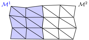
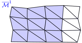
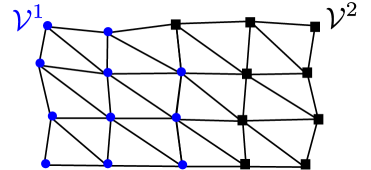
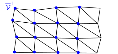
Figure 5: Example of mesh decomposition.

The partitioning of the mesh is performed by the master process (process 1), and then, each local mesh is distributed to its process. Therefore, each MPI process contains the local mesh ($\overline{{\cal M}}^{p}$, $\overline{\cal V}^{p}$, $\overline{\cal F}_{\Gamma}^{p}$), $p=1,2,...,N_{p}$ which is splitted into two parts:

$$\begin{split}&\text{own mesh: }({\cal M}^{p},{\cal V}^{p},{\cal F}_{\Gamma}^{p}),\\ &\text{ghost mesh: }(\overline{{\cal M}}^{p}\backslash{\cal M}^{p},\overline{\cal V}^{p}\backslash{\cal V}^{p},\overline{\cal F}_{\Gamma}^{p}\backslash{\cal F}_{\Gamma}^{p}).\end{split}$$

We now turn to the parallel implementation of the discrete hybrid dimensional Darcy flow model (8) and transport model (19).

4.2 Parallelization of the discrete hybrid dimensional Darcy flow

On each process $p=1,...,N_{p}$, the local problem of the discrete hybrid dimensional Darcy flow (8) is defined by the set of unknowns $u_{\mu}$, $\mu\in\overline{\cal V}^{p}\cup\overline{\cal F}_{\Gamma}^{p}\cup\overline{\cal M}^{p}$ and the set of equations

$$\left\{\begin{array}[]{r@{\,\,}c@{\,\,}ll}&&\displaystyle\sum_{{\bf s}\in{{\cal V}}_{K}}F_{K,{\bf s}}(u_{\cal D})+\sum_{\sigma\in{{\cal F}}_{\Gamma,K}}F_{K,\sigma}(u_{\cal D})=0,\,\,K\in\overline{{\cal M}}^{p},\\ &&\displaystyle\sum_{{\bf s}\in{{\cal V}}_{\sigma}}F_{\sigma,{\bf s}}(u_{\cal D})+\sum_{K\in{\cal M}_{\sigma}}-F_{K,\sigma}(u_{\cal D})=0,\,\,\sigma\in\mathcal{F}_{\Gamma}^{p},\\ &&\displaystyle\sum_{K\in{\cal M}_{s}}-F_{K,{\bf s}}(u_{\cal D})+\sum_{\sigma\in{\cal F}_{\Gamma,{\bf s}}}-F_{\sigma,{\bf s}}(u_{\cal D})=0,\,\,{\bf s}\in{\cal V}_{int}\cap\mathcal{V}^{p},\\ &&u_{\bf s}=\bar{u}_{\bf s},\,\,{\bf s}\in{\cal V}_{ext}\cap\mathcal{V}^{p}.\end{array}\right.$$ (25)

Note that this includes the equations of the nodes ${\bf s}\in\mathcal{V}^{p}$, of the fracture faces $\sigma\in\mathcal{F}_{\Gamma}^{p}$ and of the cells $K\in\overline{{\cal M}}^{p}$, both those own cells in $K\in{{\cal M}}^{p}$ and the ghost cells $K\in\overline{{\cal M}}^{p}\setminus{{\cal M}}^{p}$. The set of equations can be rewritten as the following rectangular linear system

$$\begin{pmatrix}A_{vv}^{p}&A_{vf}^{p}&A_{vc}^{p}\\ A_{fv}^{p}&A_{ff}^{p}&A_{fc}^{p}\\ A_{cv}^{p}&A_{cf}^{p}&A_{cc}^{p}\end{pmatrix}\begin{pmatrix}\overline{U}_{v}^{p}\\ \overline{U}_{f}^{p}\\ \overline{U}_{c}^{p}\end{pmatrix}=\begin{pmatrix}b_{v}^{p}\\ b_{f}^{p}\\ \overline{b}_{c}^{p}\end{pmatrix}$$ (26)

where $\overline{U}_{v}^{p}\in\mathbb{R}^{\overline{\mathcal{V}}^{p}}$, $\overline{U}_{f}^{p}\in\mathbb{R}^{\overline{\mathcal{F}}_{\Gamma}^{p}}$ and $\overline{U}_{c}^{p}\in\mathbb{R}^{\overline{{\cal M}}^{p}}$ denote the vector of process $p$ own and ghost unknowns at nodes, fracture faces and cells respectively. The above matrices have the following sizes

$$A_{vv}^{p}\in\mathbb{R}^{\mathcal{V}^{p}\times\overline{\mathcal{V}}^{p}},\ A_{vf}^{p}\in\mathbb{R}^{\mathcal{V}^{p}\times\overline{\mathcal{F}}_{\Gamma}^{p}},\ A_{vc}^{p}\in\mathbb{R}^{\mathcal{V}^{p}\times\overline{{\cal M}}^{p}},$$

$$A_{fv}^{p}\in\mathbb{R}^{\mathcal{F}_{\Gamma}^{p}\times\overline{\mathcal{V}}^{p}},\ A_{ff}^{p}\in\mathbb{R}^{\mathcal{F}_{\Gamma}^{p}\times\overline{\mathcal{F}}_{\Gamma}^{p}},\ A_{fc}^{p}\in\mathbb{R}^{\mathcal{F}_{\Gamma}^{p}\times\overline{{\cal M}}^{p}},$$

$$A_{cv}^{p}\in\mathbb{R}^{\overline{{\cal M}}^{p}\times\overline{\mathcal{V}}^{p}},\ A_{cf}^{p}\in\mathbb{R}^{\overline{{\cal M}}^{p}\times\overline{\mathcal{F}}_{\Gamma}^{p}},\ A_{cc}^{p}\in\mathbb{R}^{\overline{{\cal M}}^{p}\times\overline{{\cal M}}^{p}}.$$

and $b_{v}^{p}\in\mathbb{R}^{{\mathcal{V}}^{p}}$, $b_{f}^{p}\in\mathbb{R}^{{\mathcal{F}}_{\Gamma}^{p}}$, $\overline{b}_{c}^{p}\in\mathbb{R}^{\overline{{\cal M}}^{p}}$ denote the corresponding right hand side vectors. The matrix $A_{cc}^{p}$ is a non singular diagonal matrix and the cell unknowns can be easily eliminated without fill-in leading to the following Schur complement system

$${A}^{p}\begin{pmatrix}\overline{U}_{v}^{p}\\ \overline{U}_{f}^{p}\end{pmatrix}={b}^{p}$$ (27)

with

$$A^{p}:=\begin{pmatrix}A_{vv}^{p}&A_{vf}^{p}\\ A_{fv}^{p}&A_{ff}^{p}\end{pmatrix}-\begin{pmatrix}A_{vc}^{p}\\ A_{fc}^{p}\end{pmatrix}(A_{cc}^{p})^{-1}\begin{pmatrix}A_{cv}^{p}&A_{cf}^{p}\end{pmatrix},\ b^{p}:=\begin{pmatrix}b_{v}^{p}\\ b_{f}^{p}\end{pmatrix}-\begin{pmatrix}A_{vc}^{p}\\ A_{fc}^{p}\end{pmatrix}(A_{cc}^{p})^{-1}\overline{b}_{c}^{p},$$

and

$$\overline{U}_{c}^{p}=(A_{cc}^{p})^{-1}(b_{c}^{p}-A_{cv}^{p}\overline{U}_{v}^{p}-A_{cf}^{p}\overline{U}_{f}^{p}).$$ (28)

The linear system (27) is built locally on each process $p$ and transfered to the parallel linear solver library PETSc [7] or Trilinos [27]. The parallel matrix and the parallel vector in PETSc or Trilinos are stored in a distributed manner, i.e. each process stores its own rows. We construct the following parallel linear system

$$AU=b,$$ (29)

with

$$A:=\begin{pmatrix}A^{1}R^{1}\\ A^{2}R^{2}\\ \vdots\\ A^{N_{p}}R^{N_{p}}\end{pmatrix}\begin{array}[]{l}\big{\}}\text{ process 1}\\ \big{\}}\text{ process 2}\\ \quad\quad\vdots\\ \big{\}}\text{ process }N_{p}\end{array},\quad U:=\begin{pmatrix}U_{v}^{1}\\ U_{f}^{1}\\ U_{v}^{2}\\ U_{f}^{2}\\ \vdots\end{pmatrix}\begin{array}[]{l}\bigg{\}}\text{ process 1}\\ \bigg{\}}\text{ process 2}\\ \quad\quad\vdots\end{array},\quad b:=\begin{pmatrix}b^{1}\\ b^{2}\\ \vdots\\ b^{N^{p}}\end{pmatrix}\begin{array}[]{l}\big{\}}\text{ process 1 }\\ \big{\}}\text{ process 2 }\\ \quad\quad\vdots\\ \big{\}}\text{ process }N_{p}\end{array}$$

where $R^{p},p=1,2,...,N_{p}$ is a restriction matrix satisfying

$$R^{p}U=\begin{pmatrix}\overline{U}_{v}^{p}\\ \overline{U}_{f}^{p}\end{pmatrix}.$$

The matrix $A^{p}R^{p}$, the vector $\begin{pmatrix}U_{v}^{p}\\ U_{f}^{p}\end{pmatrix}$ and the vector $b^{p}$ are stored in process $p$.

The parallel linear system (29) is solved using the GMRES or BiCGStab algorithm preconditioned by different type of preconditioners as discussed in the numerical section. The solution of the linear system provides on each process $p$ the solution vector $\begin{pmatrix}U_{v}^{p}\\ U_{f}^{p}\end{pmatrix}$ of own node and fracture-face unknowns. Then, the ghost node unknowns $u_{\mu}$, $\mu\in(\overline{\cal V}^{p}\backslash{\cal V}^{p})$ and the ghost fracture-face unknowns $u_{\mu}$, $\mu\in(\overline{\cal F}_{\Gamma}^{p}\backslash{\cal F}_{\Gamma}^{p})$ are recovered by a synchronization step with MPI communications. This synchronization is efficiently implemented using a PETSc or Trilinos matrix vector product

$$\overline{U}=SU$$ (30)

where

$$\overline{U}:=\begin{pmatrix}\overline{U}_{v}^{1}\\ \overline{U}_{f}^{1}\\ \overline{U}_{v}^{2}\\ \overline{U}_{f}^{2}\\ \vdots\end{pmatrix}$$

is the vector of own and ghost node and fracture-face unknowns on all processes. The matrix $S$, containing only $0$ and $1$ entries, is assembled once and for all at the beginning of the simulation.

Finally, thanks to (28), the vector of own and ghost cell unknowns $\overline{U}_{c}^{p}$ is computed locally on each process $p$.

In conclusion, the parallel implementation of the discrete hybrid dimensional Darcy flow can be summarized as:

1:  Assemble locally on each process the rectangular linear system (26),

2:  Compute locally on each process the Schur complement (27) of (26),

3:  Construct the parallel linear system (29) in PETSc or Trilinos,

4:  Solve the parallel linear system (29) to obtain the solution at own nodes and fracture faces,

5:  Communicate the solution at ghost nodes and fracture faces from (30),

6:  Compute locally on each process the solution at own and ghost cells from (28).

Algorithm 1 Parallel implementation of the discrete hybrid dimensional Darcy flow

4.3 Parallelization of the discrete hybrid dimensional transport model

The parallel implementation of the transport model (19) with an explicit upwind discretization of the fluxes consists of the following four steps.

1. Compute the Darcy matrix and fracture fluxes defined by (21) and (22).

2. Compute the maximum time step $\Delta t$ satisfying the CFL condition (24) and set $\Delta t^{n}=\Delta t$ for all $n=0,\cdots,N-2$, and $\Delta t^{N-1}=T-(N-1)\Delta t$ with $N=\lceil{T\over\Delta t}\rceil$.

3. For each time step $n=0,1,...,N-2$,

   1. Compute $c_{{\bf s}}^{n+1}$, $c_{\sigma}^{n+1}$ and $c_{K}^{n+1}$, ${\bf s}\in{\cal V}_{int}\cap\mathcal{V}^{p}$, $\sigma\in\mathcal{F}_{\Gamma}^{p}$, $K\in\overline{{\cal M}}^{p}$ solution of the following explicit equations

      $$\left\{\begin{array}[]{r@{\,\,}c@{\,\,}ll}&&\displaystyle\phi_{K}{c_{K}^{n+1}-c_{K}^{n}\over\Delta t}+\sum_{{\bf s}\in{{\cal V}}_{K}}H_{K,{\bf s}}(c_{\cal D}^{n})+\sum_{\sigma\in{{\cal F}}_{\Gamma,K}}H_{K,\sigma}(c_{\cal D}^{n})=0,\,\,K\in\overline{{\cal M}}^{p},\\ &&\displaystyle\phi_{\sigma}{c_{\sigma}^{n+1}-c_{\sigma}^{n}\over\Delta t}+\sum_{{\bf s}\in{{\cal V}}_{\sigma}}H_{\sigma,{\bf s}}(c_{\cal D}^{n})-\sum_{K\in{\cal M}_{\sigma}}H_{K,\sigma}(c_{\cal D}^{n})=0,\,\,\sigma\in\mathcal{F}_{\Gamma}^{p},\\ &&\displaystyle\phi_{\bf s}{c_{{\bf s}}^{n+1}-c_{{\bf s}}^{n}\over\Delta t}-\sum_{K\in{\cal M}_{\bf s}}H_{K,{\bf s}}(c_{\cal D}^{n})-\sum_{\sigma\in{\cal F}_{\Gamma,{\bf s}}}H_{\sigma,{\bf s}}(c_{\cal D}^{n})=0,\,\,{\bf s}\in{\cal V}_{int}\cap\mathcal{V}^{p},\\ &&c_{\bf s}=\bar{c}_{\bf s},\,\,{\bf s}\in{\cal V}_{ext}\cap\mathcal{V}^{p}.\end{array}\right.$$ (31)

   2. Get the node and fracture-face ghost unknowns $c_{{\bf s}}^{n+1}$, $c_{\sigma}^{n+1}$, ${\bf s}\in{\cal V}_{int}\cap(\overline{\mathcal{V}}^{p}\backslash\mathcal{V}^{p})$, $\sigma\in\overline{\mathcal{F}}_{\Gamma}^{p}\backslash\mathcal{F}_{\Gamma}^{p}$ using the PETSc or Trilinos matrix vector product with the matrix $S$ defined in (30), as was done for the Darcy flow solution $U$:

      $$\begin{pmatrix}\overline{C}_{v}^{1}\\ \overline{C}_{f}^{1}\\ \overline{C}_{v}^{2}\\ \overline{C}_{f}^{2}\\ \vdots\end{pmatrix}=S\begin{pmatrix}C_{v}^{1}\\ C_{f}^{1}\\ C_{v}^{2}\\ C_{f}^{2}\\ \vdots\end{pmatrix}$$

Thanks to our mesh decomposition, step 1 and step 3a are performed locally on each process. For step 2, the maximum time step $\Delta t^{p}$ is computed locally on each process $p$, then the time step $\Delta t$ is obtained using the MPI reduce operation.

5 Numerical experiments

All the numerical tests have been implemented on the Cicada cluster of the University Nice Sophia Antipolis consisting of 72 nodes (16 cores/node, Intel Sandy Bridge E5-2670, 64GB/node). We always fix 1 core per process and 16 processes per node. The communications are handled by OpenMPI 1.8.2 (GCC 4.9) and PETSc 3.5.3.

The first two test cases are designed in order to validate the Darcy fluxes and the convergence of the transport model discretization on two analytical solutions including one fracture for the first test case and four intersecting fractures for the second test case. In the remaining test cases, the parallel scalability of our Darcy flow and transport solvers is assessed with different types of fracture networks and meshes and different matrix fracture permeability ratios. In particular, the last test case applies our algorithm to a complex fracture network with hundreds of fractures.

5.1 Numerical convergence for an analytical solution with one fracture

Let us set $\Omega=(0,1)^{2}$, and denote by $(x,y)$ the Cartesian coordinates of ${\bf x}$. We then define ${\bf x}_{1}=(0,{1\over 4})$, $\theta\in(0,\mbox{arctan}({3\over 4}))$, ${\bf x}_{2}=(1,{1\over 4}+\tan(\theta))$. Let $\Omega_{1}=\{(x,y)\in\Omega\,|\,y>{1\over 4}+x\tan(\theta)\}$, and $\Omega_{2}=\Omega\setminus\overline{\Omega}_{1}$. We consider a single fracture defined by $\Gamma=({\bf x}_{1},{\bf x}_{2})=\partial\Omega_{1}\cap\partial\Omega_{2}$ with tangential permeability $\Lambda_{f}>0$, and width $d_{f}>0$. The matrix permeability is isotropic and set to $\Lambda_{m}=1$, the matrix and fracture porosities are set to $\phi_{m}=\phi_{f}=1$, and the fluid viscosity is set to $\mu=1$. The pressure solution is fixed to $u(x,y)=1-x$. In this case, the transport model (19) reduces to the following system of equations which specifies our choice of the boundary and initial conditions:

$$\left\{\begin{array}[]{r@{\,\,}c@{\,\,}ll}\partial_{t}c_{m,\alpha}(x,y,t)+\partial_{x}c_{m,\alpha}(x,y,t)&=&0&\mbox{ on }\Omega_{\alpha}\times(0,T),\,\alpha=1,2,\\ c_{m,\alpha}(x,y,0)&=&0&\mbox{ on }\Omega_{\alpha},\,\alpha=1,2,\\ c_{m,1}(0,y,t)&=&1&\mbox{ on }({1\over 4},1)\times(0,T),\\ c_{m,2}(0,y,t)&=&1&\mbox{ on }(0,{1\over 4})\times(0,T),\\ c_{m,2}(x,{1\over 4}+x\tan(\theta),t)&=&c_{f}(x,t)&\mbox{ on }(0,1)\times(0,T),\\ {\cal L}c_{f}(x,t)&=&\beta c_{m,1}(x,{1\over 4}+x\tan(\theta),t)&\mbox{ on }(0,1)\times(0,T),\\ c_{f}(0,t)&=&1&\mbox{ on }(0,T),\\ c_{f}(x,0)&=&0&\mbox{ on }(0,1),\end{array}\right.$$ (40)

where ${\cal L}=\partial_{t}+k\partial_{x}+\beta$ with $\beta={\sin(\theta)\over d_{f}}$ and $k=\Lambda_{f}\cos^{2}(\theta)$. It is assumed that $k>1$. This system can be integrated along the characteristics of the matrix and fracture velocity fields leading to the following analytical solution:

$$c_{m,1}(x,y,t)=\left\{\begin{array}[]{r@{\,\,}c@{\,\,}ll}&0&\mbox{if}&t<x,\\ &1&\mbox{if}&t>x,\end{array}\right.$$

$$c_{f}(x,t)=\left\{\begin{array}[]{r@{\,\,}c@{\,\,}ll}&0&\mbox{if}&t<{x\over k},\\ &e^{-{\beta\over k-1}(x-t)}&\mbox{if}&{x\over k}<t<x,\\ &1&\mbox{if}&t>x,\end{array}\right.$$

$$c_{m,2}(x,y,t)=\left\{\begin{array}[]{r@{\,\,}c@{\,\,}l}&&\mbox{ if }y\in(0,{1\over 4})\left\{\begin{array}[]{r@{\,\,}c@{\,\,}ll}&0&\mbox{if}&t<x,\\ &1&\mbox{if}&t>x,\end{array}\right.\\ &&\mbox{ if }y\in({1\over 4},{1\over 4}+\tan(\theta))\left\{\begin{array}[]{r@{\,\,}c@{\,\,}ll}&0&\mbox{if}&t<x-{4y-1\over 4\tan(\theta)},\\ &c_{f}({4y-1\over 4\tan(\theta)},t+{4y-1\over 4\tan(\theta)}-x)&\mbox{if}&t>x-{4y-1\over 4\tan(\theta)}.\end{array}\right.\end{array}\right.$$

In the following numerical experiments the parameters are set to $\tan(\theta)={1\over 2}$, $\Lambda_{f}=20$ and $d_{f}=0.01$. The mesh is a topologically Cartesian $n_{x}\times n_{x}$ grid. Figure 6 shows an example of the mesh with $n_{x}=20$ as well as the analytical solution in the matrix obtained at time $t_{f}=0.5$ chosen as the final time of the simulation. The time step is defined by the maximum time step allowed by the CFL condition (24). Figure 8 exhibits the convergence of the relative $L^{1}$ errors between the analytical solution and the numerical solution at time $t_{f}$ both in the matrix domain and in the fracture as a function of the grid size $n_{x}=100,200,400,800,1600$. Figure 7 shows the analytical solution and the numerical solutions obtained at time $t_{f}$ along the fracture. In both cases, we can observe the expected convergence of the numerical solution to the analytical solution with a higher order of convergence in the fracture due to the fact that at time $t_{f}$ the analytical solution in the fracture is continuous as exhibited in Figure 7.

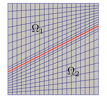
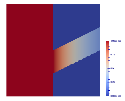
Figure 6: Left: example of mesh with $n_{x}=20$ where the red line is the fracture. Right: analytical solution of (40) at time $t_{f}=0.5$.

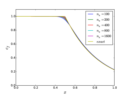
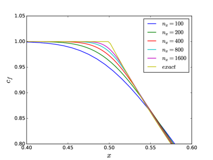
Figure 7: Left: analytical solution and numerical solutions along the fracture at time $t_{f}$ with $n_{x}=100,200,400,800,1600$. Right: zoom view of left figure around $x=0.5$.

Figure 8: Relative $L^{1}$ errors and references in the matrix domain and in the fracture at time $t_{f}$ between the analytical solution and the numerical solutions as a function of the grid size $n_{x}=100,200,400,800,1600$.

5.2 Numerical convergence for an analytical solution with four intersecting fractures

Let $\Omega=(0,1)^{2}$, ${\bf x}_{1}=(0,{1\over 4})$, $\theta_{1}\in(0,\mbox{arctan}({3\over 4}))$, ${\bf x}_{2}=(1,{1\over 4}+\tan(\theta_{1}))$, ${\bf x}_{3}=({3\over 4},0)$, ${\bf x}_{4}=({3\over 4}-\tan(\theta_{2}),1)$, and the intersection of ${\bf x}_{1}{\bf x}_{2}$ and ${\bf x}_{3}{\bf x}_{4}$ equal to

$${\bf x}_{0}=(x_{0},y_{0})={1\over 4(1+\tan(\theta_{1})\tan(\theta_{2}))}(3-\tan(\theta_{2}),1+3\tan(\theta_{1})).$$

It is assumed that $\theta_{1},\theta_{2}\in(0,\mbox{arctan}({3\over 4}))$.

We consider the four fractures $\Gamma_{1}=({\bf x}_{1},{\bf x}_{0})$, $\Gamma_{2}=({\bf x}_{0},{\bf x}_{2})$, $\Gamma_{3}=({\bf x}_{3},{\bf x}_{0})$, $\Gamma_{4}=({\bf x}_{0},{\bf x}_{4})$, with tangential permeabilities $\Lambda_{f,1}=\Lambda_{f,2}>0$, and $\Lambda_{f,3}=\Lambda_{f,4}>0$, and with widths $d_{f,1}=d_{f,2}>0$, and $d_{f,3}=d_{f,4}>0$. It is assumed that $\Lambda_{m}=1$.

The fractures partition the domain $\Omega$ in the following four subdomains

$$\Omega_{1}=\{{\bf x}=(x,y)\in\Omega\,|\,y>{1\over 4}+x\tan(\theta_{1}),x<{3\over 4}-y\tan(\theta_{2})\},$$

$$\Omega_{2}=\{{\bf x}=(x,y)\in\Omega\,|\,y>{1\over 4}+x\tan(\theta_{1}),x>{3\over 4}-y\tan(\theta_{2})\},$$

$$\Omega_{3}=\{{\bf x}=(x,y)\in\Omega\,|\,y<{1\over 4}+x\tan(\theta_{1}),x<{3\over 4}-y\tan(\theta_{2})\},$$

$$\Omega_{4}=\{{\bf x}=(x,y)\in\Omega\,|\,y<{1\over 4}+x\tan(\theta_{1}),x>{3\over 4}-y\tan(\theta_{2})\}.$$

Let us set $\beta_{1}={\sin(\theta_{1})\over d_{f,1}}$, $k_{1}=\Lambda_{f,1}\cos^{2}(\theta_{1})$, $\beta_{2}={\cos(\theta_{2})\over d_{f,3}}$, $k_{2}=\Lambda_{f,3}\cos(\theta_{2})\sin(\theta_{2})$, $r={\Lambda_{f,3}d_{f,3}\sin(\theta_{2})\over\Lambda_{f,1}d_{f,1}\cos(\theta_{1})}$. It is assumed that $k_{1}>1$ and $k_{2}\tan(\theta_{2})>1$. The matrix and fracture porosities are set to $\phi_{m}=\phi_{f}=1$ and the fluid viscosity is set to $\mu=1$.

The pressure solution is set to $u(x,y)=1-x$. In that case, the transport model (19) reduces to the following system of equations which specifies our choice of the boundary and initial conditions: find $c_{m,\alpha}(x,y,t)$, $\alpha=1,\cdots,4$, $c_{f,1}(x,t)$, $c_{f,2}(x,t)$, $c_{f,3}(y,t)$, $c_{f,4}(y,t)$, and $c_{0}(t)$ such that

$$\left\{\begin{array}[]{r@{\,\,}c@{\,\,}ll}\partial_{t}c_{m,\alpha}(x,y,t)+\partial_{x}c_{m,\alpha}(x,y,t)&=&0&\mbox{ on }\Omega_{\alpha}\times(0,T),\,\alpha=1,\cdots,4,\\ c_{m,\alpha}(x,y,0)&=&0&\mbox{ on }\Omega_{\alpha},\,\alpha=1,\cdots,4,\\ c_{m,1}(0,y,t)&=&0&\mbox{ on }({1\over 4},1)\times(0,T),\\ c_{m,3}(0,y,t)&=&0&\mbox{ on }(0,{1\over 4})\times(0,T),\\ c_{m,2}({3\over 4}-y\tan(\theta_{2}),y,t)&=&c_{f,4}(y,t)&\mbox{ on }(y_{0},1)\times(0,T),\\ c_{m,4}({3\over 4}-y\tan(\theta_{2}),y,t)&=&c_{f,3}(y,t)&\mbox{ on }(0,y_{0})\times(0,T),\\ c_{m,3}(x,{1\over 4}+x\tan(\theta_{1}),t)&=&c_{f,1}(x,t)&\mbox{ on }(0,x_{0})\times(0,T),\\ c_{m,4}(x,{1\over 4}+x\tan(\theta_{1}),t)&=&c_{f,2}(x,t)&\mbox{ on }(x_{0},1)\times(0,T),\\ {\cal L}_{1}c_{f,1}(x,t)-\beta_{1}c_{m,1}(x,{1\over 4}+x\tan(\theta_{1}),t)&=&0&\mbox{ on }(0,x_{0})\times(0,T),\\ {\cal L}_{1}c_{f,2}(x,t)-\beta_{1}c_{m,2}(x,{1\over 4}+x\tan(\theta_{1}),t)&=&0&\mbox{ on }(x_{0},1)\times(0,T),\\ {\cal L}_{2}c_{f,3}(y,t)-\beta_{2}c_{m,3}({3\over 4}-y\tan(\theta_{2}),y,t)&=&0&\mbox{ on }(0,y_{0})\times(0,T),\\ {\cal L}_{2}c_{f,4}(y,t)-\beta_{2}c_{m,1}({3\over 4}-y\tan(\theta_{2}),y,t)&=&0&\mbox{ on }(y_{0},1)\times(0,T),\\ c_{f,2}(x_{0},t)=c_{f,3}(y_{0},t)&=&c_{0}(t)&\mbox{ on }(0,T),\\ (r+1)c_{0}(t)-c_{f,1}(x_{0},t)-rc_{f,4}(y_{0},t)&=&0&\mbox{ on }(0,T),\\ c_{f,1}(0,t)=c_{f,4}(1,t)&=&1&\mbox{ on }(0,T),\\ c_{f,1}(x,0)&=&0&\mbox{ on }(0,x_{0}),\\ c_{f,2}(x,0)&=&0&\mbox{ on }(x_{0},1),\\ c_{f,3}(y,0)&=&0&\mbox{ on }(0,y_{0}),\\ c_{f,4}(y,0)&=&0&\mbox{ on }(y_{0},1),\end{array}\right.$$ (60)

where ${\cal L}_{1}=\partial_{t}+k_{1}\partial_{x}+\beta_{1}$ and ${\cal L}_{2}=\partial_{t}-k_{2}\partial_{y}+\beta_{2}$.

This system can also be integrated analytically along the characteristics of the matrix and fracture velocity fields, but it leads to complex computations. It is much easier to obtain the stationary solution of this system which is defined in the fractures by

$$c_{f,1}(x)=e^{-{\beta_{1}\over k_{1}}x},$$

$$c_{f,4}(y)=e^{-{\beta_{2}\over k_{2}}(1-y)},$$

$$c_{0}={e^{-{\beta_{1}\over k_{1}}x_{0}}+re^{-{\beta_{2}\over k_{2}}(1-y_{0})}\over r+1},$$

$$c_{f,2}(x)=e^{-{\beta_{1}\over k_{1}}x}\Bigl{(}c_{0}e^{{\beta_{1}\over k_{1}}x_{0}}+{\beta_{1}\over k_{1}r_{1}}\Bigl{(}e^{(r_{1}x-{3\beta_{2}\over 4k_{2}})}-e^{(r_{1}x_{0}-{3\beta_{2}\over 4k_{2}})}\Bigr{)}\Bigr{)},$$

$$c_{f,3}(y)=\left\{\begin{array}[]{r@{\,\,}c@{\,\,}ll}&e^{{\beta_{2}\over k_{2}}y}\Bigl{(}c_{0}e^{-{\beta_{2}\over k_{2}}y_{0}}+{\beta_{2}\over k_{2}r_{2}}\Bigl{(}e^{(-{r_{2}\over 4}-{\beta_{1}\over 4k_{1}\tan(\theta_{1})})}-e^{(-r_{2}y_{0}-{\beta_{1}\over 4k_{1}\tan(\theta_{1})})}\Bigr{)}\Bigr{)},&\mbox{if}&y<{1\over 4},\\ &e^{{\beta_{2}\over k_{2}}y}\Bigl{(}c_{0}e^{-{\beta_{2}\over k_{2}}y_{0}}+{\beta_{2}\over k_{2}r_{2}}\Bigl{(}e^{(-r_{2}y-{\beta_{1}\over 4k_{1}\tan(\theta_{1})})}-e^{(-r_{2}y_{0}-{\beta_{1}\over 4k_{1}\tan(\theta_{1})})}\Bigr{)}\Bigr{)}&\mbox{if}&y>{1\over 4},\end{array}\right.$$

with $r_{1}={\beta_{1}\over k_{1}}+{\beta_{2}\over k_{2}}\tan(\theta_{1})$ and $r_{2}={\beta_{2}\over k_{2}}+{\beta_{1}\over k_{1}\tan(\theta_{1})}$, and in the matrix by

$$c_{m,1}(x,y)=0,$$

$$c_{m,2}(x,y)=c_{f,4}(y),$$

$$c_{m,3}(x,y)=\left\{\begin{array}[]{r@{\,\,}c@{\,\,}ll}&0&\mbox{if}&y<{1\over 4},\\ &c_{f,1}\Bigl{(}{y-{1\over 4}\over\tan(\theta_{1})}\Bigr{)}&\mbox{if}&y>{1\over 4},\end{array}\right.$$

$$c_{m,4}(x,y)=\left\{\begin{array}[]{r@{\,\,}c@{\,\,}ll}&c_{f,3}(y)&\mbox{if}&y<y_{0},\\ &c_{f,2}\Bigl{(}{y-{1\over 4}\over\tan(\theta_{1})}\Bigr{)}&\mbox{if}&y>y_{0}.\end{array}\right.$$

In the following numerical experiments the parameters are set to $\tan(\theta_{1})={5\over 8}$, $\tan(\theta_{2})={1\over 4}$, $\Lambda_{f,1}=200$, $\Lambda_{f,3}=400$, and $d_{f,1}=d_{f,3}=0.01$. The mesh is, as for the previous test case, a topologically Cartesian $n_{x}\times n_{x}$ grid exhibited in Figure 9 for $n_{x}=20$. Figure 9 also shows the stationary analytical solution in the matrix. The time step is again defined by the maximum time step allowed by the CFL condition (24) and the simulation time is chosen large enough to obtain the numerical stationary solution.

Figure 10 exhibits the convergence of the relative $L^{1}$ errors between the stationary analytical and the numerical solutions both in the matrix domain and in the fracture as a function of the grid size $n_{x}=100,200,400,800$. We can again observe the expected convergence of the numerical solution to the analytical solution with a higher order of convergence in the fracture network due to the fact that the solution is continuous on each individual fracture as exhibited in Figure 10. This property is always true when looking at the solution at the matrix time scale and could be exploited in a future work by using an implicit time integration in the fracture coupled to an explicit time integration in the matrix domain with a higher order discretization in space in the spirit of what has been done in [29].

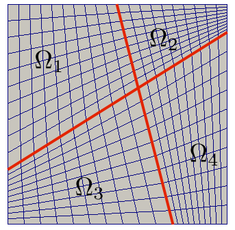
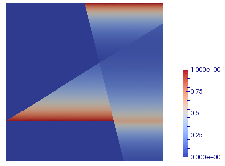
Figure 9: Left: example of mesh with $n_{x}=20$ where the red lines account for the four fractures. Right: stationary analytical solution of (60).

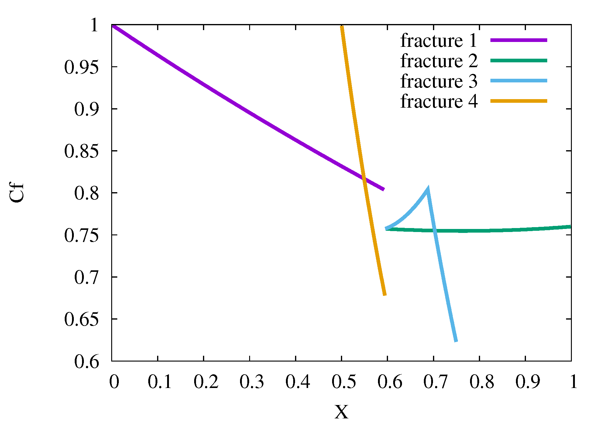
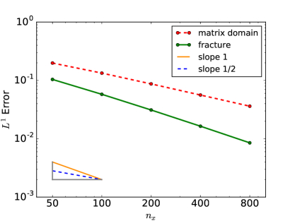
Figure 10: Left: stationary analytical solution in the four fractures as a function of the $x$ coordinate. Right: relative $L^{1}$ errors and references in the matrix domain and in the fracture network between the stationary analytical and numerical solutions as a function of the grid size $n_{x}=100,200,400,800$.

5.3 Fracture network with hexahedral meshes

The objective of this subsection and of the next subsection is to investigate the parallel scalability of the algorithms described in Section 4. In this subsection we consider a topologically Cartesian mesh of size $n_{x}\times n_{x}\times n_{x}$ of the cubic domain $(0,1)^{3}$ exhibited in Figure 11 for $n_{x}=32$. The mesh is exponentially refined at the interface between the matrix and the fracture network exhibited in Figure 12. The permeabilities are isotropic and set to $\Lambda_{f}=20$ in the fracture network and to $\Lambda_{m}=1$ in the matrix. The porosities are set to $\phi_{m}=\phi_{f}=1$ and the fluid viscosity is set to $\mu=1$. The initial concentration is set to $0$ both in the matrix domain and in the fracture network and a value of $1$ of the concentration is injected on the bottom boundaries of the matrix and of the fracture network. The pressure is fixed to $u=1$ and $\gamma u=1$ on the bottom boundary and to $u=0$ and $\gamma u=0$ on the top boundary. The remaining lateral boundaries are considered impervious. Figure 12 exhibits the tracer concentrations obtained with the mesh $n_{x}=128$ at times $t=0$, $t=0.2$, $t=0.4$ and at the final simulation time $t_{f}=0.5$.

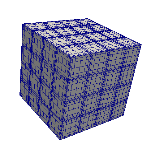
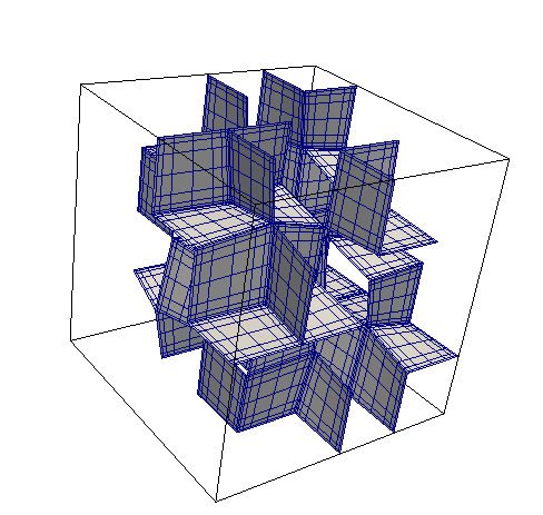
Figure 11: Hexahedral mesh in the matrix domain (left) and in the fracture network (right) with $n_{x}=32$.

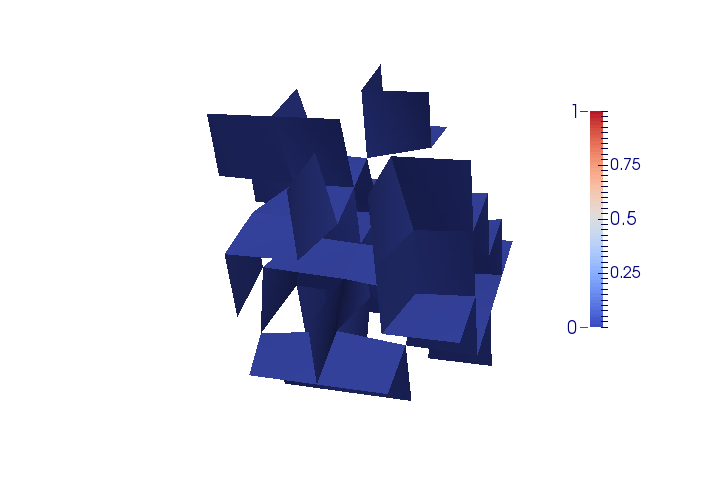
(a) $t=0.0$

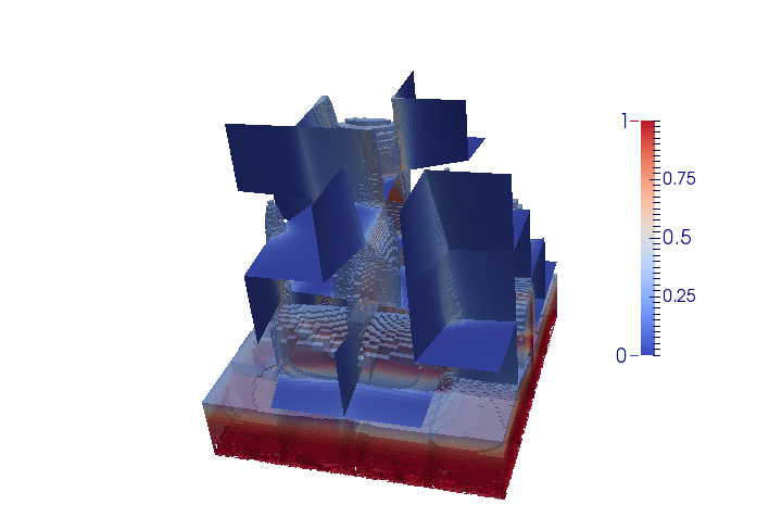
(b) $t=0.2$

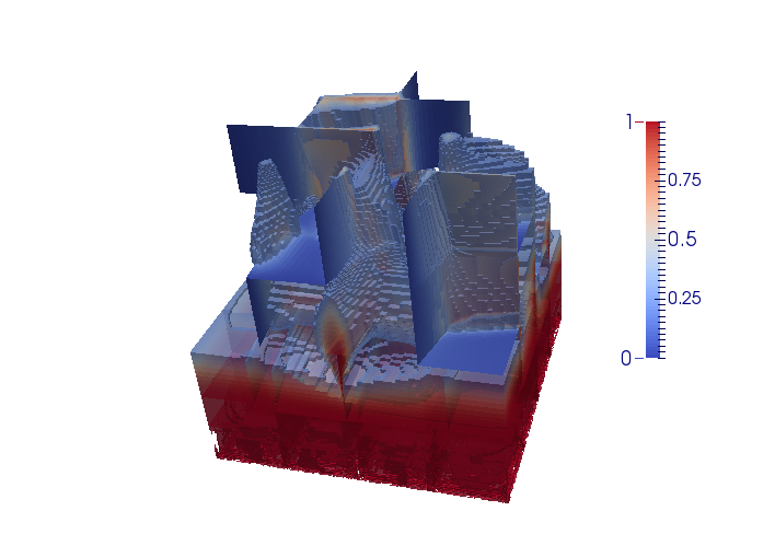
(c) $t=0.4$

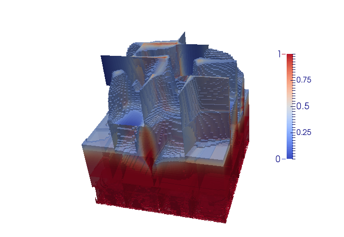
(d) $t=0.5$

Figure 12: Concentration in the matrix domain and in the fracture network obtained at different times with the mesh $n_{x}=128$. A threshold concentration of 0.2 is used in the matrix domain.

Table 1 presents the numbers of linear solver iterations for the stationary pressure solution for a number of MPI processes ranging from $N_{p}=2$ to $N_{p}=512$ and with the mesh size $n_{x}=128$ corresponding to roughly $2.1\times 10^{6}$ cells, $2.1\times 10^{6}$ nodes and $5.2\times 10^{4}$ fractures faces. Both the GMRES and BiCGStab linear solvers from the PETSc library are tested combined with either the Boomer AMG preconditioner from the Hypre library [30], the Aggregation AMG preconditioner from the Trilinos library [27] or the block Jacobi ILU(0) preconditioner from the Euclid library. No restart is used for the GMRES linear solver. Table 5.3 shows the corresponding computation times both for the setup phase of the preconditioner and for the solve phase of the linear solver.

According to these tables, the GMRES and the BiCGStab linear solvers combined with the Boomer AMG preconditioner are good choices for a number of processes $N_{p}\leqslant 128$, while the BiCGStab linear solver combined with the block Jacobi ILU(0) preconditioner is more efficient for this test case for $N_{p}=256$ and $N_{p}=512$. This was expected since the Boomer AMG preconditioner requires a sufficiently large number of unknowns per core to maintain a good parallel scalability due to the high level of communications in particular in the setup phase of the preconditioner. For this linear system, the number of unknowns per MPI process is roughly $4100$ for $N_{p}=512$ which is too small for this type of preconditioner while the block Jacobi preconditioner still maintains a good parallel scalability for such a number of unknowns per MPI process. On the other hand, as shown in Table 3, Boomer AMG exhibits an optimal scalability while ILU(0) is not scalable in terms of iteration count with respect to the ratio ${\Lambda_{f}\over\Lambda_{m}}$ between the fracture and matrix permeabilities. The same remark also holds in terms of scalability with respect to the mesh size which means that the ILU(0) preconditioner is only advantageous for small size and mildly heterogeneous problems.

Tables 1 and 5.3 also clearly show that the BiCGStab linear solver outperforms the GMRES linear solver for cases requiring a large number of iterations due to the fact that the cost of the orthogonalization procedure increases with the dimension of the Krylov subspace. The Aggregation AMG preconditioner yields a larger number of iterations compared with the Boomer AMG preconditioner but has a much lower setup time resulting for this test case in a total lower CPU time. However, this implementation of the Aggregation AMG preconditioner seems to lack robustness with respect to the matrix fracture permeability ratio as exhibited in Table 3.

Table 1: Number of linear solver iterations vs. the number of MPI processes obtained with different linear solvers and preconditioners for the mesh size $n_{x}=128$.

$N_{p}$	2	4	8	16	32	64	128	256	512
GMRES + Boomer AMG	15	15	15	15	15	16	15	15	15
GMRES + Aggregation AMG	59	78	65	39	65	54	73	53	62
GMRES + ILU(0)	751	707	655	644	648	634	633	624	613
BiCGStab + Boomer AMG	9	9	9	9	9	10	9	9	10
BiCGStab + ILU(0)	508	476	484	503	473	513	491	487	484

Table 2: Linear solver setup phase and solve phase computation times vs. the number of MPI processes obtained with different linear solvers and preconditioners for the mesh size $n_{x}=128$.

$N_{p}$		2	4	8	16	32	64	128	256	512
GMRES Boomer AMG	Setup	34.1	20.1	16.3	11.7	11.3	11.9	12.1	19.2	29.3
	Solve	26.3	15.6	14.8	7.2	5.2	3.8	2.5	5.2	9.6
GMRES Aggregation AMG	Setup	4.7	1.9	1.6	1.5	2.3	2.9	4.4	6.6	11.3
	Solve	45.1	20.9	17.0	9.7	5.2	2.5	2.3	1.5	3.2
GMRES ILU(0)	Setup	16.9	21.3	16.3	23.2	14.6	11.0	9.7	6.0	4.8
	Solve	672.3	590.9	281.6	163.9	71.4	30.7	16.7	8.3	4.0
BiCGStab Boomer AMG	Setup	38.0	23.3	15.0	10.3	9.1	9.4	12.8	14.8	23.8
	Solve	37.1	21.3	11.5	7.4	4.1	2.9	2.5	4.4	10.0
BiCGStab ILU(0)	Setup	18.9	19.9	16.5	22.1	14.3	12.4	9.4	5.8	3.9
	Solve	179.4	111.7	86.0	59.9	27.9	15.4	8.0	4.2	2.2

Next, Figure 13 plots the total (Darcy flow and transport models) computation time and the computation time for the transport model only as a function of the number of processes. In these runs the GMRES linear solver is used combined with the Boomer AMG preconditioner for $N_{p}\leqslant 128$ and with the ILU(0) preconditioner for $N_{p}=256,512$. For the range $2-512$ of the number of processes, it appears that the computation time of the Darcy flow linear system solution remains small compared with the transport model computation time. This can be checked by comparison of the computation times in Table 5.3 and in Figure 13. This explains the good scalability obtained for both the total and transport computation times thanks to the explicit nature of the time integration scheme.

Table 3: Number of linear solver iterations vs. the matrix fracture permeability ratio ${\Lambda_{f}\over\Lambda_{m}}$ for $n_{x}=128$ and $N_{p}=2,128$.

	$N_{p}=2$			$N_{p}=128$
$\Lambda_{f}/\Lambda_{m}$	20	100	1000	20	100	1000
GMRES + Boomer AMG	15	15	16	15	15	15
GMRES + Aggregation AMG	59	-	-	73	-	-
GMRES + ILU(0)	751	-	-	633	-	-

• -: The solver doesn’t converge in 1200 iterations.

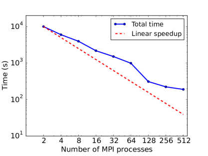
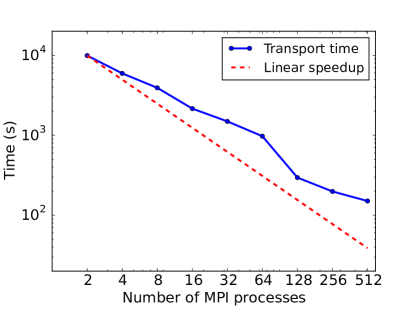
Figure 13: Total computation time (left) and computation time for the transport model (right) vs. the number of MPI processes for the mesh size $n_{x}=128$.

5.4 Fracture network with tetrahedral meshes

This test case considers tetrahedral meshes of the cubic domain $(0,1)^{3}$ conforming to the fracture network. An example of tetrahedral mesh showing both the matrix domain and the fracture network is exhibited in Figure 14. All the physical parameters, initial and boundary conditions are the same as for the previous test case. The mesh used in this subsection contains about $6.2\times 10^{6}$ cells, $9.7\times 10^{5}$ nodes and $7.1\times 10^{4}$ fracture faces. Figure 15 exhibits the tracer concentrations obtained with this tetrahedral mesh at times $t=0$, $t=0.2$, $t=0.4$ and at the final simulation time $t_{f}=0.5$.

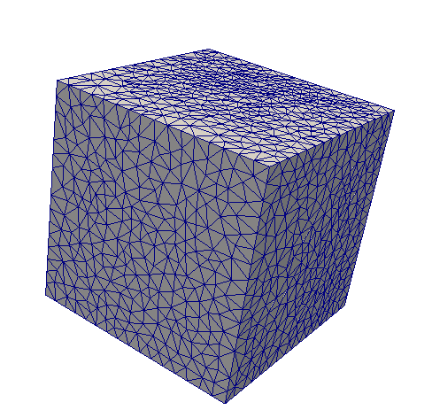
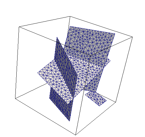
Figure 14: Example of tetrahedral mesh of the matrix domain (left) conforming to the fracture network (right).

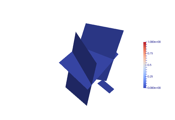
(c) $t=0.0$

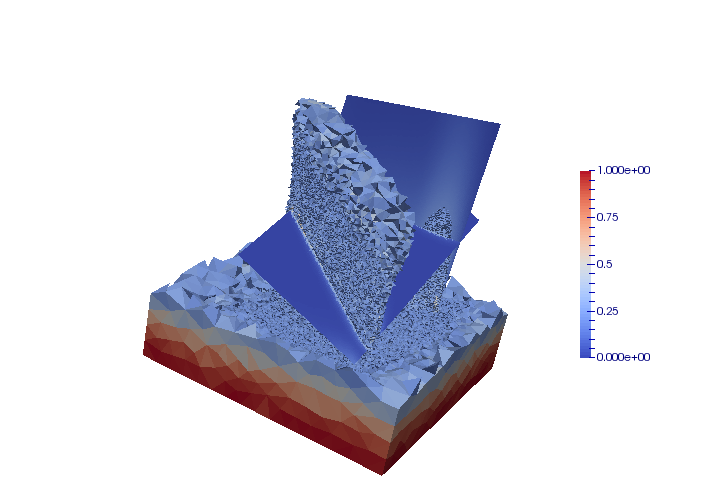
(d) $t=0.2$

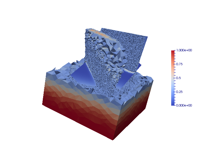
(e) $t=0.4$

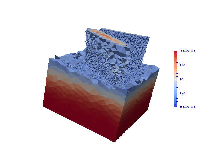
(f) $t=0.5$

Figure 15: Concentration in the matrix domain and in the fracture network obtained at different times for the tetrahedral mesh. A threshold of 0.2 is used in the matrix domain.

As for the previous test case, Tables 4, 5.4 and 6 investigate the performance of the Darcy flow system linear solution for both the GMRES and BiCGStab linear solvers and for the same three preconditioners as in the previous test case. The conclusions are basically the same as for the hexahedral mesh test case. The Boomer AMG preconditioner exhibits an optimal robustness with respect to the matrix fracture permeability ratio ${\Lambda_{f}\over\Lambda_{m}}$. On the other hand it requires a rather high number of unknowns per MPI process to maintain a good parallel scalability due to the high level of communications in particular in the setup phase. The ILU(0) preconditioner can be an interesting alternative but only for small size and midly heterogeneous problems. The aggregation AMG preconditioner from the Trilinos library used in our test cases seems to lack robustness and we did not manage to make it work better through tuning its parameters.

Table 4: Number of linear solver iterations vs. the number of MPI processes obtained with different linear solvers and preconditioners for the tetrahedral mesh.

$N_{p}$	2	4	8	16	32	64	128	256	512
GMRES + Boomer AMG	11	12	12	12	12	12	12	12	12
GMRES + Aggregation AMG	38	78	40	39	52	-	35	-	52
GMRES + ILU(0)	1003	725	717	682	667	656	644	629	612
BiCGStab + Boomer AMG	8	7	8	8	8	8	8	8	8
BiCGStab + ILU(0)	565	513	527	544	535	483	489	483	473

• -: The relative residual norm stagnates after a few iterations.

• -: Some future investigations are necessary.

Table 5: Linear solver setup phase and solve phase computation times vs. the number of MPI processes obtained with different linear solvers and preconditioners for the tetrahedral mesh.

$N_{p}$		2	4	8	16	32	64	128	256	512
GMRES Boomer AMG	Setup time	12.4	7.8	4.9	5.0	4.3	6.2	7.2	13.5	22.4
	Solve time	8.0	5.5	2.9	1.7	1.1	0.9	1.4	3.1	6.9
GMRES Aggregation AMG	Setup time	3.7	1.9	1.2	1.8	2.1	1.6	2.9	3.3	4.7
	Solve time	19.7	20.9	5.1	2.7	2.0	-	1.5	-	3.0
GMRES ILU(0)	Setup time	5.7	7.4	7.2	5.6	4.7	5.2	3.4	2.8	1.8
	Solve time	560.6	254.4	150.0	66.5	30.1	15.2	7.7	4.1	2.8
BiCGStab Boomer AMG	Setup time	21.5	14.5	9.9	6.5	5.3	5.9	8.2	12.4	19.7
	Solve time	24.0	10.2	6.1	3.5	1.8	1.5	2.1	4.3	9.5
BiCGStab ILU(0)	Setup time	5.8	6.4	6.4	5.4	4.7	5.0	3.4	2.6	1.8
	Solve time	110.4	63.0	39.0	19.2	11.6	5.4	2.8	1.4	1.2

• -: The residual norm stagnates after a few iterations.

Table 6: Number of linear solver iterations vs. the matrix fracture permeability ratio ${\Lambda_{f}\over\Lambda_{m}}$ for the tetrahedral mesh and $N_{p}=2,128$.

	$N_{p}=2$			$N_{p}=128$
$\Lambda_{f}/\Lambda_{m}$	20	100	1000	20	100	1000
GMRES + Boomer AMG	11	13	12	12	13	12
GMRES + Aggregation AMG	38	-	-	35	-	-
GMRES + ILU(0)	1002	-	-	644	-	-

• -: The solver doesn’t converge in 1200 iterations.

Figure 16 plots the total (Darcy flow and transport models) computation time and the computation time of the transport model only as a function of the number of processes. In these runs the GMRES linear solver is used combined with the Boomer AMG preconditioner for $N_{p}\leqslant 128$ and with the ILU(0) preconditioner for $N_{p}=256,512$. Compared with the previous subsection, an even better parallel scalability of the transport model computation time is observed in the right Figure 16. This can be explained by the ratio of roughly $6$ between the number of cells and the number of nodes typical of a tetrahedral mesh. For a topologically Cartesian mesh, this ratio is roughly $1$. Since the cell concentrations are computed locally in each process, this explains the better scalability observed for this tetrahedral mesh compared with the previous hexahedral mesh. On the left Figure 16, it is observed that the linear system solution computation time is no longer small compared with the transport computation time for $N_{p}=256$ and $512$. Hence, it significantly reduces the parallel efficiency of the simulation for a large number of processes, say $N_{p}=256,512$ in this test case.

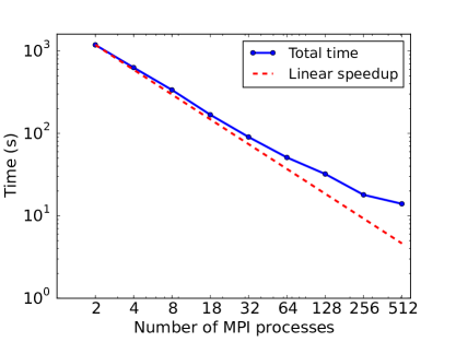
Figure 16: Total computation time (left) and computation time for transport model (right) vs. number of MPI processes with tetrahedral mesh.

5.5 Application to a complex fracture network

In this subsection, our algorithm is applied to a complex fracture network kindly provided by M. Karimi-Fard and A. Lapène from Stanford University and TOTAL. Figure 17 exhibits the mesh of the domain $\Omega=(0,5888.75)\times(0,3157.5)\times(0,250)$ (m) which contains about $1.2\times 10^{7}$ prismatic cells, $6.5\times 10^{6}$ nodes and $5.13\times 10^{5}$ fracture faces. This 3D mesh is defined by the tensor product of a triangular 2D mesh with a uniform vertical 1D mesh with $24$ intervals. The fracture network exhibited in Figure 18 contains 581 connected components. It is a set of $21376\times 24$ faces of the 3D mesh defined by the tensor product of a subset of $21376$ edges of the triangular 2D mesh with the 1D vertical mesh. The 2D triangular mesh contains $517540$ cells and is refined in the neighbourhood of the fracture network down to an average size of $3.5$ m. Figure 18 also shows the location of the injection well and of the two production wells. Each well is vertical of radius $r_{w}=0.1$ m and its centre in the horizontal plane is located at the middle of a fracture edge in the 2D triangular mesh. In the vertical direction, only the $12$ fracture faces at the center of the 1D mesh are perforated. The permeabilities are isotropic and set to $\Lambda_{f}=10^{-11}$ ($m^{2}$) in the fracture network and to $\Lambda_{m}=10^{-15}$ ($m^{2}$) in the matrix domain. The porosities are set to $\phi_{m}=\phi_{f}=0.1$, the fracture width to $d_{f}=1$ m and the fluid viscosity to $\mu=10^{-3}$ Pa.s^-1.

The initial concentration is set to $0$ both in the matrix domain and in the fracture network. A total volume of $5.0\times 10^{6}$ m³ is injected in one year at the injector well with a tracer concentration of $1$. The pressures of each perforated fracture face $\sigma$ of the producer wells are fixed to $p_{w}=0$ and the flow rates are given by the Peaceman model q_σ= WI_σ(p_σ-p_w), where $p_{\sigma}$ is the pressure in the fracture face and $WI_{\sigma}$ the well index of the fracture face. This well index is computed following Peaceman methodology [36], [37], [14] by expanding the fracture face as a box of size $dx\times d_{f}\times dz$. The analytical pressure solution obtained for a vertical well with the well pressure $p_{w}$, the well radius $r_{w}$ and the well flow rate $q_{w}$ per unit length is imposed at the 8 corners of the box. Then, the flow rate $q_{w}dz$ is imposed at the box center and the pressure $p_{c}$ at the box center can be computed analytically using the VAG scheme. We deduce the well index WI = q_w dz pc-pw leading in this simple case to the analytical formula WI = 2 πdz Λ_f log(r0rw) with r_0 = D exp( -2πdz C), and C = 4 3( dx dz df + dx d_f dz + dz d_f dx ),  D = 0.5 dx^2 + d_f^2 . The production lasts $8$ years.

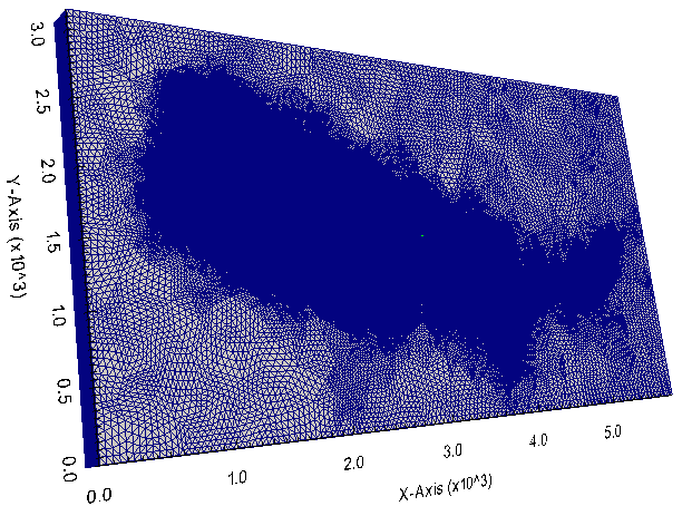
Figure 17: Prismatic mesh of the domain $\Omega$ defined by the tensor product of a vertical 1D uniform mesh with a 2D triangular mesh.

Figure 18: Fracture network showing the location of the single injection well and of the two production wells.

Figure 19 plots the mean tracer concentration in each well as a function of time as well as the total volume of tracer as a function of time in the matrix, in the fracture network and their sum. Figure 20 exhibit the pressure solution in the matrix domain and Figures 21 and 22 shows the tracer concentration after one year of injection and at final time both in the matrix domain and in the fracture network.

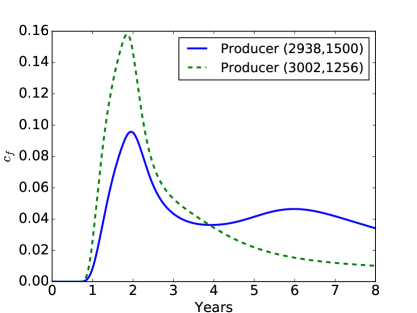
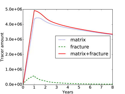
Figure 19: Mean tracer concentration in both production wells as a function of time (left) defined as the ratio between the well tracer flow rate and the well fluid flow rate (equal in our case to the well fracture-face tracer concentration). Volume of tracer as a function of time in the matrix domain, in the fracture network and their sum (right).

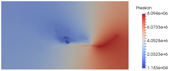
Figure 20: Pressure on the matrix domain.

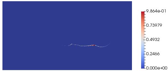
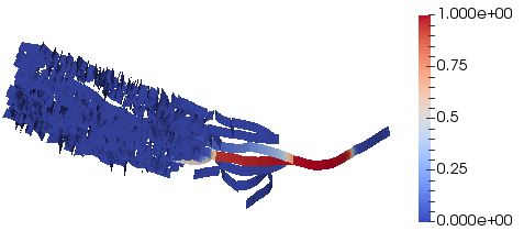
Figure 21: Tracer concentration after one year of injection in the matrix domain (left) and in the fracture network (right).

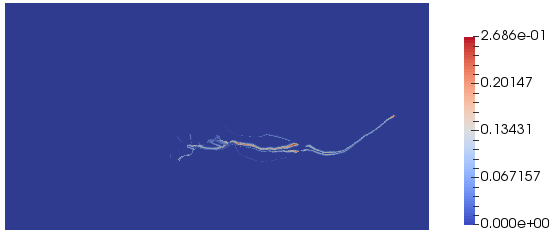
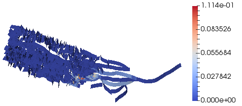
Figure 22: Tracer concentration at final time in the matrix domain (left) and in the fracture network (right).

Figure 23 shows the total computation times with different number of MPI processes $N_{p}=16,32,64,128,256,512$. It is observed that the total computation time exhibits a rather good scalability. In addition, the linear solver (GMRES+Boomer AMG) for the pressure converges in no more than 25 iterations whatever the number of MPI processes. Also the comparison of the total and transport computation times in Figure 23 shows that the time for the pressure solution remains small compared with the transport computation time up to $N_{p}=512$.

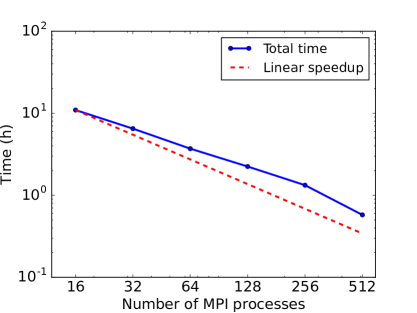
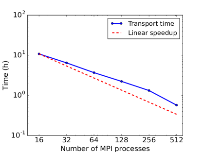
Figure 23: Total computation time in hours (left) and computation time for transport model (right) vs. number of MPI processes with prismatic mesh.

6 Conclusion

This paper introduced a parallel VAG scheme for the simulation of a hybrid dimensional Darcy flow and transport model in a discrete fracture network taking into account the mass exchanges with the matrix. The convergence of the scheme was validated on two original analytical solutions for a flow and transport model that includes fractures. The parallel efficiency of the algorithm was studied for different complexities of fracture networks, and a large range of matrix fracture permeability ratios and different type of meshes. The numerical results exhibit a very good parallel strong scalability as expected from the explicit nature of the time integration of the transport model with a better result on tetrahedral meshes thanks to the communication free computation of the cell unknowns. The Darcy flow solution is remarkably robust using the Boomer AMG preconditioner on all types of fracture networks, meshes and for all permeability ratios that have been tested. On the other hand, it requires as usual a rather high number of unknowns per process to maintain a good parallel scalability. Future work includes the extension of the parallel algorithm to hybrid dimensional multiphase flow models and the use of a more accurate second order MUSCL scheme for the transport model.

Acknowledgments

This work is supported by a joint project between INRIA and BRGM Carnot institutes (ANR, INRIA, BRGM). This work was also granted access to the HPC and visualization resources of “Centre de Calcul Interactif” hosted by University Nice Sophia Antipolis. This work was partially funded by ADEME BRGM research project Orbou (convention 1305C0131). We would like also to thank Mohammad Karimi-Fard and Alexandre Lapène for kindly providing us the mesh of Section 5.5.

References

- [1] Ahmed, R., Edwards, M.G., Lamine, S., Huisman, B.A.H., Pal, M.: Control-volume distributed multi-point flux approximation coupled with a lower-dimensional fracture model. Journal of Computational Physics 284, 462-489 (2015)
- [2] Ahmed, R., Edwards, M.G., Lamine, S., Huisman, B.A.H., Pal, M.: Three-dimensional control-volume distributed multi-point flux approximation coupled with a lower-dimensional surface fracture model. Journal of Computational Physics 303, 470-497 (2015)
- [3] Alboin, C., Jaffré, J., Roberts, J.E., Serres, C.: Modeling fractures as interfaces for flow and transport in porous media. Fluid flow and transport in porous media 295, 13-24 (2002)
- [4] Amir, L., Kern, M., Martin, V., Roberts, J.E.: Décomposition de domaine et préconditionnement pour un modèle 3D en milieu poreux fracturé Proceeding of JANO 8. 8th conference on Numerical Analysis and Optimization, (2005)
- [5] Angot, P., Boyer, F., Hubert, F.: Asymptotic and numerical modelling of flows in fractured porous media. ESAIM Mathematical Modelling and Numerical Analysis 23, 239-275 (2009)
- [6] Antonietti, P.F., Formaggia, L., Scotti, A., Verani, M., Verzott, N.: Mimetic finite difference approximation of flows in fractured porous media. ESAIM Mathematical Modelling and Numerical Analysis 50, 809-832 (2016)
- [7] Balay, S., Adams, M., Brown, J., Brune, P., Buschelman, K., Eijkhout, V., Zhang, H.: PETSc Users Manual. Revision 3.5 (2015)
- [8] Berrone, S., Pieraccini, S., Scialò, S.: An optimization approach for large scale simulations of discrete fracture network flows. Journal of Computational Physics 256, 838-853 (2014)
- [9] Bogdanov, I.I., Mourzenko, V.V., Thovert, J.-F., Adler, P.M.: Two-phase flow through fractured porous media. Physical Review E 68, 026703 (2003)
- [10] Brenner, K., Masson, R.: Convergence of a vertex centered discretization of two-phase Darcy flows on general meshes. International Journal of Finite Volume Methods, june (2013)
- [11] Brenner, K., Groza, M., Guichard, C., Masson, R.: Vertex approximate gradient scheme for hybrid dimensional two-phase Darcy flows in fractured porous media. ESAIM Mathematical Modelling and Numerical Analysis 49, 303-330 (2015)
- [12] Brenner, K., Groza, M., Guichard, C., Lebeau, G., Masson, R.: Gradient discretization of hybrid dimensional Darcy flows in fractured porous media. Numerische Mathematik, 1-41 (2015)
- [13] Brenner, K., Hennicker, J., Masson, R., Samier, P.: Gradient discretization of hybrid dimensional Darcy flows in fractured porous media with discontinuous pressure at matrix fracture interfaces. IMA Journal of Numerical Analysis, published online september 28 (2016)
- [14] Chen, Z., Zhang, Y.: Well flow models for various numerical methods. International Journal of Numerical Analysis and Modeling 6(3), 375-388 (2009)
- [15] Dalissier, E., Guichard, C., Havé, P., Masson, R., Yang, C.: ComPASS: a tool for distributed parallel finite volume discretizations on general unstructured polyhedral meshes. ESAIM: Proceedings 43, 147-163 (2013)
- [16] D’Angelo, C., Scotti, A.: A mixed finite element method for Darcy flow in fractured porous media with non-matching grids. ESAIM Mathematical Modelling and Numerical Analysis 46(2) 465-489 (2012)
- [17] Droniou, J., Eymard, R., Gallouët, T., Herbin, R.: Gradient schemes: A generic framework for the discretisation of linear, nonlinear and nonlocal elliptic and parabolic equations. Mathematical Models and Methods in Applied Sciences 23(13), 2395-2432 (2013)
- [18] Droniou, J., Eymard, R., Gallouët, T., Guichard, C., Herbin, R.: The Gradient discretization method: A framework for the discretization of linear and nonlinear elliptic and parabolic problems. Preprint https://hal.archives-ouvertes.fr/hal-01382358, (2016)
- [19] Eymard, R., Guichard, C., Herbin, R.: Small-stencil 3D schemes for diffusive flows in porous media. Mathematical Modelling and Numerical Analysis 46, 265-290 (2010)
- [20] Eymard, R., Herbin, R., Guichard, C., Masson, R.: Vertex centred discretization of compositional multiphase Darcy flows on general meshes. Computational Geosciences 16(4) 987-1005 (2012)
- [21] Eymard, R., Guichard, C., Masson, R.: High performance computing linear algorithms for two-phase flow in porous media. FVCA 7 Proceedings, (2014)
- [22] Flauraud, E., Nataf, F., Faille, I., Masson, R.: Domain Decomposition for an asymptotic geological fault modeling, Comptes Rendus à l’académie des Sciences de Mécanique 331, 849-855 (2003)
- [23] Faille, I., Fumagalli, A., Jaffré, J., Roberts, J.E.: Model reduction and discretization using hybrid finite volumes of flow in porous media containing faults. Computational Geosciences 20, 317-339 (2016)
- [24] Formaggia, L., Fumagalli, A., Scotti, A., Ruffo, P.: A reduced model for Darcy’s problem in networks of fractures. ESAIM Mathematical Modelling and Numerical Analysis 48(4), 1089-1116 (2014)
- [25] Fumagalli, A., Scotti, A.: A reduced model for flow and transport in fractured porous media with non-matching grids. Numerical Mathematics and Advanced Applications 2011, 499-507 (2013)
- [26] Haegland, H.: Streamline methods with application to flow and transport in fractured media. PhD thesis, University of Bergen (2009)
- [27] Heroux M. A., Willenbring J. M.: Trilinos Users Guide. (2003)
- [28] Geiger, S., Huangfu, Q., Reid, F., Matthai, S., Coumou D., Belayneh, M., Fricke, C., Schmid, K.: Massively parallel sector scale discrete fracture and matrix simulation. Society of Petroleum Engineers (2009)
- [29] Hoteit, J., Firoozabadi, A.: An efficient numerical model for incompressible two-phase flow in fracture media. Advances in Water Resources 31, 891-905, (2008)
- [30] Hypre - Parallel high performance preconditioners, http://acts.nersc.gov/hypre.
- [31] Karimi-Fard, M., Durlofsky, L.J., Aziz, K.: An efficient discrete-fracture model applicable for general-purpose reservoir simulators. Society of Petroleum Engineers, (2004)
- [32] Karypis, G., Kumar, V.: A fast and high quality multilevel scheme for partitioning irregular graphs. SIAM Journal on Scientific Computing 20(1), 359-392 (1998)
- [33] Martin, V., Jaffré, J., Roberts, J.E.: Modeling fractures and barriers as interfaces for flow in porous media. SIAM Journal on Scientific Computing 26(5), 1667-1691 (2005)
- [34] Matthai, S.K., Mezentsev, M.A, Belayneh, M.A: Finite element-node-centred finite-volume two-phase-flow experiments with fractured rock represented by hybrid-element. SPE Reservoir Evaluation & Engineering 12, 740-756 (2007)
- [35] Monteagudu, J., Firoozabadi, A.: Control-volume model for simulation of water injection in fractured media: incorporating matrix heterogeneity and reservoir wettability effects. SPE Journal 12(03), 355-366 (2007)
- [36] Peaceman, D.W.: Interpretation of well-block pressures in numerical reservoir simulation. SPE Journal 18(03), 183-94, (1978)
- [37] Peaceman, D.W.: Interpretation of well-block pressures in numerical reservoir simulation with nonsquare grid blocks and anisotropic permeability. SPE Journal 23(03), 531-43, (1983)
- [38] Reichenberger, V., Jakobs, H., Bastian, P., Helmig, R.: A mixed-dimensional finite volume method for multiphase flow in fractured porous media. Advances in Water Resources 29(7), 1020-1036 (2006)
- [39] Sandve, T.H., Berre, I., Nordbotten, J.M.: An efficient multi-point flux approximation method for discrete fracture-matrix simulations. Journal of Computational Physics 231, 3784-3800 (2012)
- [40] Schwenck, N., Flemisch, B., Helmig, R., Wohlmuth, B.: Dimensionally reduced flow models in fractured porous media: crossings and boundaries. Computational Geosciences 19, 1219-1230 (2015)
- [41] Si, H.: http://tetgen.org
- [42] Tunc, X., Faille, I., Gallouët, T., Cacas, M.C., Havé, P.: A model for conductive faults with non matching grids. Computational Geosciences 16, 277-296 (2012)