High performance Python for direct numerical simulations of turbulent flows

Abstract

Direct Numerical Simulations (DNS) of the Navier Stokes equations is an invaluable research tool in fluid dynamics. Still, there are few publicly available research codes and, due to the heavy number crunching implied, available codes are usually written in low-level languages such as C/C++ or Fortran. In this paper we describe a pure scientific Python pseudo-spectral DNS code that nearly matches the performance of C++ for thousands of processors and billions of unknowns. We also describe a version optimized through Cython, that is found to match the speed of C++. The solvers are written from scratch in Python, both the mesh, the MPI domain decomposition, and the temporal integrators. The solvers have been verified and benchmarked on the Shaheen supercomputer at the KAUST supercomputing laboratory, and we are able to show very good scaling up to several thousand cores.

A very important part of the implementation is the mesh decomposition (we implement both slab and pencil decompositions) and 3D parallel Fast Fourier Transforms (FFT). The mesh decomposition and FFT routines have been implemented in Python using serial FFT routines (either NumPy, pyFFTW or any other serial FFT module), NumPy array manipulations and with MPI communications handled by MPI for Python (mpi4py). We show how we are able to execute a 3D parallel FFT in Python for a slab mesh decomposition using 4 lines of compact Python code, for which the parallel performance on Shaheen is found to be slightly better than similar routines provided through the FFTW library. For a pencil mesh decomposition 7 lines of code is required to execute a transform.

1 Introduction

Direct Numerical Simulations (DNS) is a term reserved for computer simulations of turbulent flows that are fully resolved in both time and space. DNS are usually conducted using numerical methods of such high order and accuracy that numerical dispersion and diffusion errors are negligible compared to their actual physical counterparts. To this end, DNS has historically been carried out with extremely accurate and efficient spectral methods, and in the fluid dynamics community DNS enjoys today the same status as carefully conducted experiments. DNS can provide detailed and highly reliable data not possible to extract from experiments, which in recent years have driven a number of discoveries regarding the very nature of turbulence. The present paper presents a new, computationally attractive tool for performing DNS, realized by recent programming technologies.

Because of the extremely heavy number crunching implied by DNS, researchers aim at highly optimized implementations running on massively parallel computing platforms. The largest known DNS simulations performed today are using hundreds of billions of degrees of freedom, see, e.g., [14, 7]. Normally, this demands a need for developing tailored, hand-tuned codes in what we here call low-level languages: Fortran, C or C++ (despite the possibility for creating high-level abstractions in Fortran 90/2003 and C++, the extreme performance demands of DNS codes naturally leads to minimalistic use of classes and modules). Few DNS codes are openly available and easily accessible to the public and the common fluid mechanics researcher. Some exceptions are hit-3d (Fortran90) [5], Philofluid (Fortran) [11], Tarang (C++) [30], and Turbo (Fortran90) [28]. However, the user interfaces to these codes are not sophisticated and user-friendly, and it is both challenging and time consuming for a user to modify or extend the codes to satisfy their own needs. This is usually the nature of codes written in low-level languages.

It is a clear trend in computational sciences over the last two decades that researchers tend to move from low-level to high-level languages like Matlab, Python, R, and IDL, where prototype solvers can be developed at greater comfort. The experience is that implementations in high-level languages are faster to develop, easier to test, easier to maintain, and they reach a much wider audience because the codes are compact and readable. The downside has been the decreased computational efficiency of high-level languages and in particular their lack of suitability for massively parallel computing. In a field like computational fluid dynamics, this argument has been a show stopper.

Python is a high-level language that over the last two decades has grown very popular in the scientific computing community. A wide range of well established, “gold standard” scientific libraries in Fortran and C have been wrapped in Python, making them directly accessible just as commands in MATLAB. There is little overhead in calling low-level Fortran and C/C++ functions from Python, and the computational speed obtained in a few lines of code may easily compete with hundreds of compiled lines of Fortran or C code. It is important new knowledge in the CFD community if flow codes can be developed with comfort and ease in Python without sacrificing much computational efficiency.

The ability of Python to wrap low-level, computationally highly efficient Fortran and C/C++ libraries for various applications is today well known, appreciated, and utilized by many. A lesser known fact is that basic scientific Python modules like NumPy (cf. [21, 29]), used for linear algebra and array manipulations, and MPI for Python (mpi4py) [18], which wraps (nearly) the entire MPI library, may be used directly to develop, from scratch, high performance solvers that run at speeds comparable to the very best implementations in low-level codes. A general misconception seems to be that Python may be used for fast prototyping and post-processing, as MATLAB, but that serious high-performance computing on parallel platforms require reimplementations in Fortran, C or C++. In this paper, we conquer this misconception: The only real requirement for developing a fast scientific Python solver is that all array manipulations are performed using vectorization (that calls underlying BLAS or LAPACK backends or compiled NumPy ufuncs) such that explicit for loops over long arrays in Python are avoided. The MPI for Python module in turn provides a message passing interface for NumPy arrays at communication speeds very close to pure C code.

There are already several examples on successful use of Python for high-performance parallel scientific computing. The sophisticated finite element framework FEniCS [10] is written mainly in C++, but most application developers are writing FEniCS-based solvers directly in Python, never actually finding themselves in need of writing longer C++ code and firing up a compiler. For large scale applications the developed Python solvers are usually equally fast as their C++ counterparts, because most of the computing time is spent within the low-level wrapped C++ functions that perform the costly linear algebra operations [17]. GPAW [16] is a code devoted to electronic structure calculations, written as a combination of Python and C. GPAW solvers written in Python have been shown to scale well for thousands of processors. The PETSc project [2] is a major provider of linear algebra to the open source community. PETSc was developed in C, but through the package PETSc for Python (petsc4py) almost all routines may be set up and called from Python. PyClaw [12] is another good example, providing a compact, powerful, and intuitive Python interface to the algorithms within the Fortran codes Clawpack and SharpClaw. PyClaw is parallelised through PETSc and has been shown to scale well up to 65,000 cores.

Python has capabilities today for providing short and quick implementations that compete with tailored implementations in low-level languages up to thousands of processors. This fact is not well known, and the purpose of this paper is to demonstrate such a result for DNS and show the technical implementation details that are needed. As such, the major objective of this work is to explain a novel implementation of an excellent research tool (DNS) aimed at a wide audience. To this end, we i) show how a complete pseudo-spectral DNS solver can be written from scratch in Python using less than 100 lines of compact, very readable code, and ii) show that these 100 lines of code can run at speeds comparable to its low-level counterpart in hand-written C++ code on thousands of processors. To establish scaling and benchmark results, we have run the codes on Shaheen, a massively parallel Blue Gene/P machine at the KAUST Supercomputing Laboratory. The code described is part of a larger DNS project and available online (https://github.com/mikaem/spectralDNS) under a GPL license.

2 The Navier-Stokes equations in spectral space

Our DNS implementation is based on a pseudo-spectral Fourier-Galerkin method [4] for the spatial discretization. The Navier-Stokes equations are first cast in rotational form

$$\frac{\partial\bm{u}}{\partial t}-\bm{u}\times\bm{\omega} =\nu\nabla^{2}\bm{u}-\nabla{P},$$ (1)

$$\nabla\cdot\bm{u} =0,$$ (2)

$$\bm{u}(\bm{x}+2\pi\bm{e}^{i},t) =\bm{u}(\bm{x},t),\quad\text{for }\,i=1,2,3,$$ (3)

$$\bm{u}(\bm{x},0) =\bm{u}_{0}(\bm{x})$$ (4)

where $\bm{u}(\bm{x},t)$ is the velocity vector, $\bm{\omega}=\nabla\times\bm{u}$ the vorticity vector, $\bm{e}^{i}$ the Cartesian unit vectors, and the modified pressure $P=p+\bm{u}\cdot\bm{u}/2$, where $p$ is the regular pressure normalized by the constant density. The equations are periodic in all three spatial directions. If all three directions now are discretized uniformly in space using a structured computational mesh with $N$ points in each direction, the mesh points can be represented as

$$\bm{x}=(x,y,z)=\Big{\{}(x_{i},y_{j},z_{k})=\left(\frac{2\pi i}{N},\frac{2\pi j}{N},\frac{2\pi k}{N}\right):\\ \,i,j,k\in 0,\ldots,N-1\Big{\}}.$$ (5)

In the spectral Galerkin method all variables must be transformed from the physical mesh $\bm{x}$ to a discrete and bounded Fourier wavenumber mesh. The three-dimensional wavenumber mesh may be represented as

$$\bm{k}=(k_{x},k_{y},k_{z})=\Big{\{}(l,m,n):\\ \,l,m,n\in-\frac{N}{2}+1,\ldots,\frac{N}{2}\Big{\}}.$$ (6)

The discrete Fourier transforms are used to move between real space $\bm{x}$ and spectral space $\bm{k}$. A component of the velocity vector (with similar notation for other field variables) is approximated in both real and spectral space as

$$u(\bm{x},t) =\frac{1}{N^{3}}\sum_{\bm{k}}\hat{u}_{\bm{k}}(t)e^{\imath\bm{k}\cdot\bm{x}},$$ (7)

$$\hat{u}_{\bm{k}}(t) =\sum_{\bm{x}}u(\bm{x},t)e^{-\imath\bm{k}\cdot\bm{x}},$$ (8)

where $\hat{u}_{\bm{k}}(t)$ is used to represent the Fourier coefficients, $\imath=\sqrt{-1}$ represents the imaginary unit, and $e^{\imath\bm{k}\cdot\bm{x}}$ represents the basis functions for the spectral Galerkin method. Equations (7) and (8) correspond, respectively, to the three-dimensional discrete Fourier transform, $\mathcal{F}$, and its inverse $\mathcal{F}^{-1}$. We use the notation

$$\hat{u}_{\bm{k}}(t)=\hat{{u}}(k_{x},k_{y},k_{z},t)=\mathcal{F}({u}(\bm{x},t))\\ \left[=\mathcal{F}_{k_{x}}\left(\mathcal{F}_{k_{y}}\left(\mathcal{F}_{k_{z}}({u})\right)\right)\right],$$ (9)

$${u}(\bm{x},t)={u}(x,y,z,t)=\mathcal{F}^{-1}(\hat{{u}}_{\bm{k}}(t))\\ \left[=\mathcal{F}^{-1}_{z}\left(\mathcal{F}^{-1}_{y}\left(\mathcal{F}^{-1}_{x}(\hat{{u}})\right)\right)\right],$$ (10)

where the indices on $\mathcal{F}$ and $\mathcal{F}^{-1}$ within the square brackets are used to indicate direction of the transform. Both forward and inverse transforms involve three consecutive transformations, one for each periodic direction. The inverse transforms must be computed in the opposite order of the forward transforms, but otherwise the order is arbitrary. The first forward transform (here in the $z$-direction) is real and the remaining two are complex valued.

The spectral Galerkin method involves taking the inner product of the Navier-Stokes equations with the basis functions, $e^{\imath\bm{k}\cdot\bm{x}}$, which corresponds to performing a three-dimensional Fourier transform of the Navier-Stokes equations. If we also evaluate the analytical spatial derivatives in spectral space, we obtain a system of ordinary differential equation for $\hat{\bm{u}}_{\bm{k}}$, whereas the continuity equation reduces to an orthogonal inner product. All in all we obtain

$$\frac{d\hat{\bm{u}}_{\bm{k}}}{dt}-\widehat{(\bm{u}\times\bm{\omega})}_{\bm{k}} =-\nu|\bm{k}|^{2}\hat{\bm{u}}_{\bm{k}}-\imath\bm{k}\hat{P}_{\bm{k}},$$ (11)

$$\imath\bm{k}\cdot\hat{\bm{u}}_{\bm{k}} =0.$$ (12)

The pressure may be eliminated by taking the divergence of (1), or equivalently by dotting the transformed (11) by $\imath\bm{k}$ and rearranging such that

$$\hat{P}_{\bm{k}}=-\frac{\imath\bm{k}\cdot\widehat{(\bm{u}\times\bm{\omega})}_{\bm{k}}}{|\bm{k}|^{2}}.$$ (13)

Inserting for the pressure in (11), the final equation to solve for the transformed velocity vector in wavenumber space is thus

$$\frac{d\hat{\bm{u}}_{\bm{k}}}{dt}=\widehat{(\bm{u}\times\bm{\omega})}_{\bm{k}}-\nu|\bm{k}|^{2}\hat{\bm{u}}_{\bm{k}}-\bm{k}\frac{\bm{k}\cdot\widehat{(\bm{u}\times\bm{\omega})}_{\bm{k}}}{|\bm{k}|^{2}}.$$ (14)

Note that the transformed velocity components are coupled through the nonlinear convection term and the eliminated pressure.

The pseudo-spectral label arises from the treatment of the convective term, which is computed by first transforming the velocity and vorticity to physical space, performing the cross product, and then transforming the vector ${(\bm{u}\times\bm{\omega})}$ back to Fourier space. The operation requires 2 inverse transforms (velocity and vorticity) and 1 forward transform for each of the three vector components, 9 all together. This is the only operation that requires MPI communication and it is typically the most computationally extensive part of a pseudo-spectral DNS solver.

The time integration of (14) is performed using an explicit method. Canuto et al. [4] provides a good discussion on many different integrators for these equations, and in the Appendix we have used a fourth-order Runge-Kutta method. For the DNS solver described here an explicit integrator is reasonable because the time step by physical measures is required to be small in order to resolve all temporal scales in the flow. And by resolving these scales the integrator is usually well within stability limits as dictated by the numerical scheme. In other words, the CFL number will usually be required to be much lower than 1 in order to resolve the temporal scales.

3 Implementation

We have implemented the pseudo-spectral discretization of the Navier-Stokes equations, as described in the previous section, in high-level Python code. A complete solver is shown in the Appendix. It is strongly remarked that this Python code is not simply a wrapper of a low-level, high-performance flow solver written originally in Fortran, C or C++. The entire code is implemented directly in Python: the mesh, the solution arrays, the MPI domain decomposition, and the time integrators. We are only making use of wrappers for serial FFT, something that is also done by the majority of low-level flow solvers anyway. The current Python implementation may, as such, be used as an easy to follow, working prototype for a complete low-level implementation in Fortran, C or C++.

The scientific Python solver makes extensive use of the NumPy and MPI for Python (mpi4py) packages, but if the pyFFTW module has been installed, this module will be used to perform the FFT instead of NumPy. Note that the pyFFTW module is a wrapper for the FFTW library (www.fftw.org), whereas NumPy wraps FFTPACK (www.netlib.org/fftpack). The program starts with importing the necessary modules and initializing MPI:

⬇

from numpy.fft import fftfreq, fft, ifft, \

irfft2, rfft2, irfftn, rfftn

from mpi4py import MPI

try:

from pyfftw.interfaces.numpy_fft \

import fft, ifft, irfft2, rfft2, \

irfftn, rfftn

except ImportError:

pass # Rely on numpy.fft routines

# Get some MPI

comm = MPI.COMM_WORLD

num_processes = comm.Get_size()

rank = comm.Get_rank()

Importing MPI from mpi4py initializes the MPI communicator. Two different strategies, slab and pencil, have been implemented for the MPI parallel domain decomposition. However, since communication only enters the solver through the FFTs (and post processing), there is very little difference between a serial code and a parallel one. Therefore, we first present a serial version of the code.

3.1 Serial version of code

The computational mesh is in physical space a structured uniform (periodic) cube $[0,2\pi]^{3}$, where each direction is divided into $N$ uniform intervals, where $N=2^{M}$ for a positive integer $M$. Any different size of the box may be easily implemented through scaling of the governing equations. The mesh according to (5) is represented in Python as

⬇

M = 6

# Actual number of nodes in each direction

N = 2**M

# Physical size of computational box

L = 2*pi

# The mesh

X = mgrid[:N, :N, :N].astype(float)*L/N

The matrix X has dimensions (3, N, N, N). Since the Navier Stokes equations are solved in Fourier space, the physical space is only used to compute the convection plus to do post processing. The mesh X is typically used for initialization and is otherwise not needed (and may therefore be deleted to save memory). In parallel mode, X will be split up and divided between the processors. Note that the solver may be operated in either single or double precision mode, and that float in our code is a placeholder for either one of the NumPy datatypes float32 or float64 (single or double precision), depending on settings.

The velocity field to be transformed is real, and the discrete Fourier transform of a real sequence has the property that $\hat{\bm{u}}_{k}=\hat{\bm{u}}_{N-k}^{*}$, where ^∗ denotes the complex conjugate. As such, it is sufficient to use $N/2+1$ Fourier coefficients in the first transformed direction, leading to a transformed wavenumber mesh of size $(N/2+1)N^{2}$. The odd number of wavenumbers does not lead to any issues for the serial version of the code or for the slab decomposition. However, for the pencil decomposition it requires special attention, see Section 3.3.

In our code the real transform is taken in the $z$ direction and the wavenumbers $\bm{k}=(k_{x},k_{y},k_{z})$ stored on the transformed mesh thus has ordering as used by the FFT routines provided by NumPy or pyFFTW:

$$\bm{k}=[ (0,\ldots,N/2-1,-N/2,-N/2+1,\ldots,-1),$$

$$(0,\ldots,N/2-1,-N/2,-N/2+1,\ldots,-1),$$

$$(0,\ldots,N/2-1,N/2)].$$ (15)

A three-dimensional wavenumber mesh is implemented as

⬇

kx = ky = fftfreq(N, 1./N).astype(int)

kz = kx[:Nf].copy(); kz[-1] *= -1

K = array(meshgrid(kx, ky, kz,

indexing=’ij’), dtype=int)

K2 = sum(K*K, 0, dtype=int)

K_over_K2 = K.astype(float) / where(

K2 == 0, 1, K2).astype(float)

where fftfreq(N, 1./N) is a function that creates the wavenumbers $(0,\ldots,N/2-1,-N/2,-N/2+1,\ldots,-1)$. The dimensions of the matrices are (3, N, N, N/2+1) for K and K_over_K2, and (N, N, N/2+1) for K2, and these matrices represent $\bm{k}$, $\bm{k}/|\bm{k}|^{2}$ and $|\bm{k}|^{2}$, respectively. The last two matrices are precomputed for efficiency.

The velocity, curl and pressure are similarily stored in structured (uninitialized) NumPy arrays

⬇

U_hat = empty((3, N, N, Nf), dtype=complex)

P = empty((N, N, N), dtype=float)

P_hat = empty((N, N, Nf), dtype=complex)

curl = empty((3, N, N, N), dtype=float)

Here hat denotes a transformed variable. To transform between, e.g., U and U_hat, calls to FFT routines are required. The three dimensional FFT and its inverse are implemented in Python functions as shown below.

⬇

"""FFT of u in three directions."""

if num_processes == 1:

fu[:] = rfftn(u, axes=(0,1,2))

return fu

def ifftn_mpi(fu, u):

"""Inverse FFT of fu in three directions."""

if num_processes == 1:

u[:] = irfftn(fu, axes=(0,1,2))

return u

# Usage

U_hat = fftn_mpi(U, U_hat)

U = ifftn_mpi(U_hat, U)

For high performance, it is key that the Python code relies on in-place modifications of pre-allocated arrays to avoid unnecessary allocation of large temporary arrays (which often arises from NumPy code with basic array arithmetics). Each of the functions above takes the result array (U_hat or U) as argument, fill this array with values and returns the array to the calling code. A commonly applied convention in Python is to return all result objects from functions as this only involves transfer of references and no copying of data.

We also remark that the three consecutive transforms performed by rfftn/irfftn are actually using one real transform along the $z$-direction and two complex transforms in the remaining two directions. Also note that the simple NumPy/pyFFTW wrapped functions rfftn/irfftn for three dimensional FFT may only be used in single processor mode, and the MPI implementation is detailed in Sections 3.2 and 3.3.

The convection term requires a transform from Fourier to physical space where the cross product $\bm{u}\times\bm{\omega}$ is carried out. The curl in Fourier space is

$$\mathcal{F}(\nabla\times\bm{u})=\hat{\bm{\omega}}_{\bm{k}}=\imath\bm{k}\times\hat{\bm{u}}_{\bm{k}}.$$ (16)

We can now compute the curl in physical space through $\bm{\omega}=\mathcal{F}^{-1}(\hat{\bm{\omega}}_{\bm{k}})$. The convection term may thus be computed as

$$\widehat{(\bm{u}\times\bm{\omega})}_{\bm{k}}=\mathcal{F}(\bm{u}\times\bm{\omega})=\mathcal{F}(\bm{u}\times\mathcal{F}^{-1}(\imath\bm{k}\times\hat{\bm{u}}_{\bm{k}})).$$ (17)

The Python functions for the curl and cross products are

⬇

c[0] = fftn_mpi(a[1]*b[2]

-a[2]*b[1], c[0])

c[1] = fftn_mpi(a[2]*b[0]

-a[0]*b[2], c[1])

c[2] = fftn_mpi(a[0]*b[1]

-a[1]*b[0], c[2])

return c

def Curl(a, c):

c[2] = ifftn_mpi(1j*(K[0]*a[1]

-K[1]*a[0]), c[2])

c[1] = ifftn_mpi(1j*(K[2]*a[0]

-K[0]*a[2]), c[1])

c[0] = ifftn_mpi(1j*(K[1]*a[2]

-K[2]*a[1]), c[0])

return c

and the computation of $\widehat{(\bm{u}\times\bm{\omega})}_{\bm{k}}$ is shown below in the Python function computeRHS. The main body of the solver, including a simple Forward Euler integrator, is implemented as:

⬇

dU = empty((3, N, Nf, N), dtype=complex)

dt = 0.01 # Time step

nu = 0.001 # Viscosity

def computeRHS(dU):

# Compute convective term

curl = Curl(U_hat, curl)

dU = Cross(U, curl, dU)

# Dealias the nonlinear convection

dU *= dealias

# Compute pressure

P_hat[:] = sum(dU*K_over_K2, 0,

out=P_hat)

# Subtract pressure gradient

dU -= P_hat*K

# Subtract viscous term

dU -= nu*K2*U_hat

return dU

t = 0 # Physical time

T = 1.0 # End time

while t <= T:

t += dt

U_hat += computeRHS(dU)*dt

for i in range(3):

U[i] = ifftn_mpi(U_hat[i], U[i])

Obviously, more advanced and accurate integrators may be easily added by modifying the final while loop. See the Appendix for a fourth order Runge Kutta implementation.

The dealias matrix multiplying dU in the above loop deserves a comment. The nonlinear convection term in (14) is here dealiased using the 2/3-rule [22] and dealiasing is then simply achieved by an elementwise multiplication of a convection matrix dU[3, N, N, N/2+1] with a matrix dealias[N, N, N/2+1], that is zero where the wavenumbers are larger than 2/3 of the Nyquist mode and unity otherwise. The relevant code to create such a matrix for dealiasing reads

⬇

dealias = array((abs(K[0]) < kmax_dealias)*

(abs(K[1]) < kmax_dealias)*

(abs(K[2]) < kmax_dealias),

dtype=bool)

Note that the dimensions of dU and dealias differ in the first index since dU contains contributions from all three vector components. However, through automatic broadcasting, NumPy realizes that the last three dimensions are the same and as such all three components of dU (i.e., dU[0], dU[1] and dU[2]) are multiplied elementwise with the same matrix dealias. Note that we have here simply described the most straightforward way of dealiasing a pseudo-spectral solver and that several more advanced and accurate methods exists, see, e.g., Canuto et al. [4].

3.2 1D Slab decomposition

To run the code on several processors using MPI, the mesh and the data structures need to be split up. The most popular strategy in the literature is the “slab” decomposition, where each CPU is assigned responsibility for a certain number of complete 2D planes (slices). In other words, just one of the three indices $(i,j,k)$ is split up and divided amongst the CPUs. The major drawback of the slab decomposition strategy is that the number of CPUs must be smaller than or equal to $N$ for a cubic mesh of size $N^{3}$. The MPI implementation in FFTW makes use of the slab decomposition strategy, but there is currently no interface from Python to these MPI routines.

The decomposed physical and wavenumber meshes for the slab decomposition are implemented through a slight modification of the serial code:

⬇

sx = slice(rank*Np, (rank+1)*Np)

X = mgrid[sx, :N, :N].astype(float)*L/N

K = array(meshgrid(kx, ky[sx], kz,

indexing=’ij’), dtype=int)

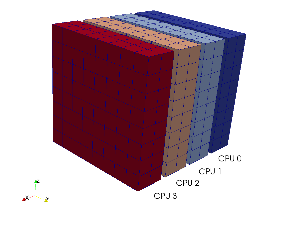
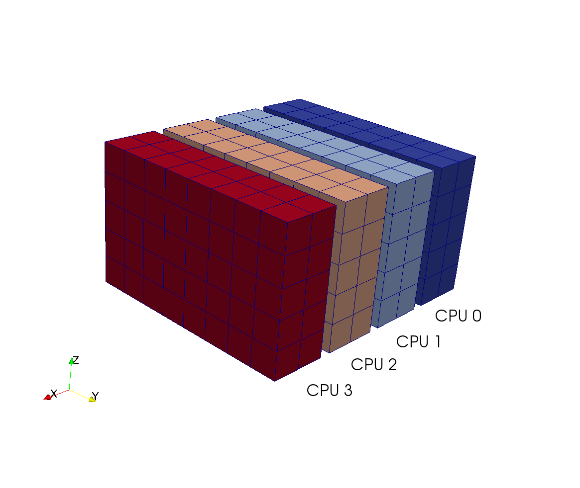
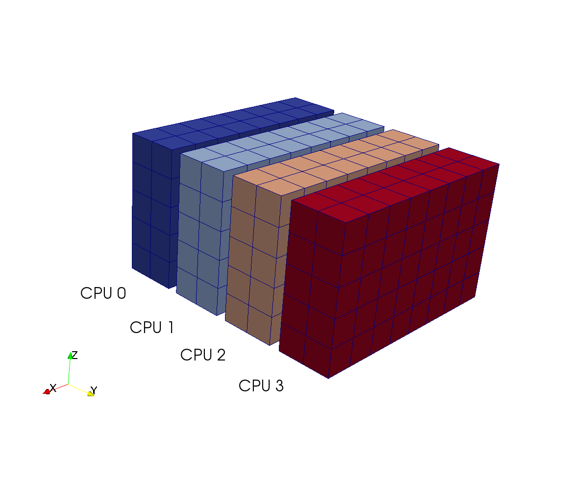
In general, using num_processes CPUs, each CPU gets responsibility for Np = N/num_processes two-dimensional slices and the physical mesh is simply decomposed along the first index. The wavenumber mesh, on the other hand, is split along the second index. The reason for this choice is that the $k_{x}$ direction is the last direction to be transformed by the three consecutive FFTs and for this operation the data structures will need to be aligned in planes normal to the $k_{y}$ direction. This becomes obvious if one considers the MPI decomposition as illustrated in Figure 2 for the case of a physical mesh of size $8^{3}$ divided amongst 4 CPUs.

The entire 3D parallel FFT may be implemented with preallocation of a work array for MPI and 4 lines (the body of fftn_mpi/ifftn_mpi) of compact Python code, see Figure 1. Also shown in Figure 1 is the parallel inverse transform.

⬇

U_mpi = empty((num_processes, Np, Np, Nf), dtype=complex)

def fftn_mpi(u, fu):

"""FFT in three directions using MPI and the slab decomposition"""

Uc_hatT = rfft2(u, axes=(1, 2))

U_mpi[:] = rollaxis(Uc_hatT.reshape(Np, num_processes, Np, Nf), 1)

comm.Alltoall([U_mpi, mpitype], [fu, mpitype])

fu[:] = fft(fu, axis=0)

return fu

def ifftn_mpi(fu, u):

"""Inverse FFT in three directions using MPI.

Need to do ifft in reversed order of fft."""

Uc_hat = ifft(fu, axis=0)

comm.Alltoall([Uc_hat, mpitype], [U_mpi, mpitype])

Uc_hatT[:] = rollaxis(U_mpi, 1).reshape(Uc_hatT.shape)

u[:] = irfft2(Uc_hatT, axes=(2, 1))

return u

Figure 1: Three dimensional forward fftn_mpi and inverse ifftn_mpi FFTs implemented for the slab decomposition.

Consider the function fftn_mpi in Figure 1. In the first call to rfft2 each processor performs a complete two dimensional FFT in both $z$ and $y$ directions on the original real data structure u (i.e., the inner $\mathcal{F}_{k_{y}}(\mathcal{F}_{k_{z}}(u))$ from (9)). The first transform, in the $z$-direction, is real to complex and the second complex to complex. The real to complex transform reduces the size of the data structure to the one seen in Figure 2(b). To be able to perform the final transform in the $x$-direction, data must be communicated between all processors. The second index of the data structure ($y$-direction, see Figure 2(c)) will now be shared amongst the processors. The line involving rollaxis is an advanced transpose operation that performs the transformation from the data structure in Figure 2(b) to the one in Figure 2(c). After the transformation the data structures have the correct shape, but they contain the wrong data. The communication of data required for the final transform takes place in one single MPI Alltoall operation, where the mpitype is a placeholder for either MPI.F_DOUBLE_COMPLEX or MPI.F_FLOAT_COMPLEX depending on settings. After this communication the data structures are lined up for the final FFT in the $x$-direction. The ifftn_mpi routine is basically the inverse of the forward transform and its implementation should be straightforward to follow.

Only one explicit global pre-allocated complex work array (U_mpi[num_processes, Np, Np, N/2+1]) is needed for the Alltoall routine in the three-dimensional FFT. The transform routines of pyFFTW maintain their own work arrays and Uc_hatT and Uc_hat above actually point to this internal data storage. Alternatively, the forward data transfer may be performed completely without explicit work arrays using the in-place Sendrecv_replace instead of Alltoall, along with transpose operations. This is easily implemented, but, since the method has been found slightly slower, details are not shown here.

(a) Physical mesh

(b) Wavenumber mesh after real transform

(c) Final wavenumber mesh.

Figure 2: Slab decomposition of physical mesh 2(a), intermediate wavenumber mesh 2(b), and final wavenumber mesh 2(c). In fftn_mpi from Figure 1 the function rfft2 transforms in $y$ and $z$-directions and moves the real data in 2(a) to the complex datastructure in 2(b). The complex data is then transposed and communicated to reach the final structure seen in 2(c).

3.3 2D Pencil decomposition

For massively parallel simulations the slab decomposition falls short since the number of CPUs allowed is limited by $N$. Large-scale simulations using up to $N^{2}$ CPUs commonly employ the 2D pencil decomposition, first suggested by Ding, Ferraro and Gennery in 1995 [8]. Publically available implementations of the 3D parallel FFT that makes use of the pencil decomposition are the Parallel FFT Subroutine Library by Plimpton [26], the P3DFFT library by Pekurovsky [23, 24], the 2DECOMP&FFT library by Li and Laizet [15] and PFFT by Pippig [25].

(a) Physical mesh

(b) Wavenumber mesh after real transform

(c) Intermediate wavenumber mesh

(d) Final wavenumber mesh.

Figure 3: 2D pencil decomposition of physical mesh 3(a) and the three wavenumber meshes 3(b), 3(c), 3(d). The decomposition shown uses 4 CPUs, two in each direction normal to the direction of the current one-dimensional FFT. The FFT in the $z$-direction transforms the real data in 3(a) to the complex data in 3(b). The data is then transformed and communicated to the composition seen in 3(c). Here the FFT in $x$-direction is carried out before the data is transformed again and communicated to 3(d), where the final FFT is performed.

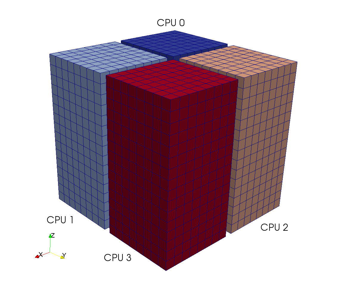
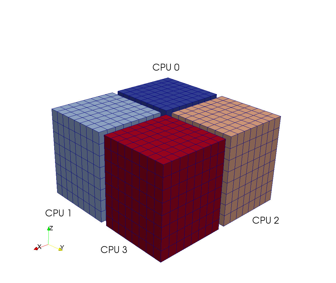
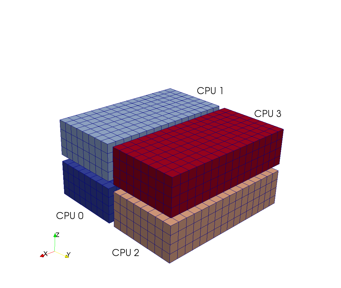
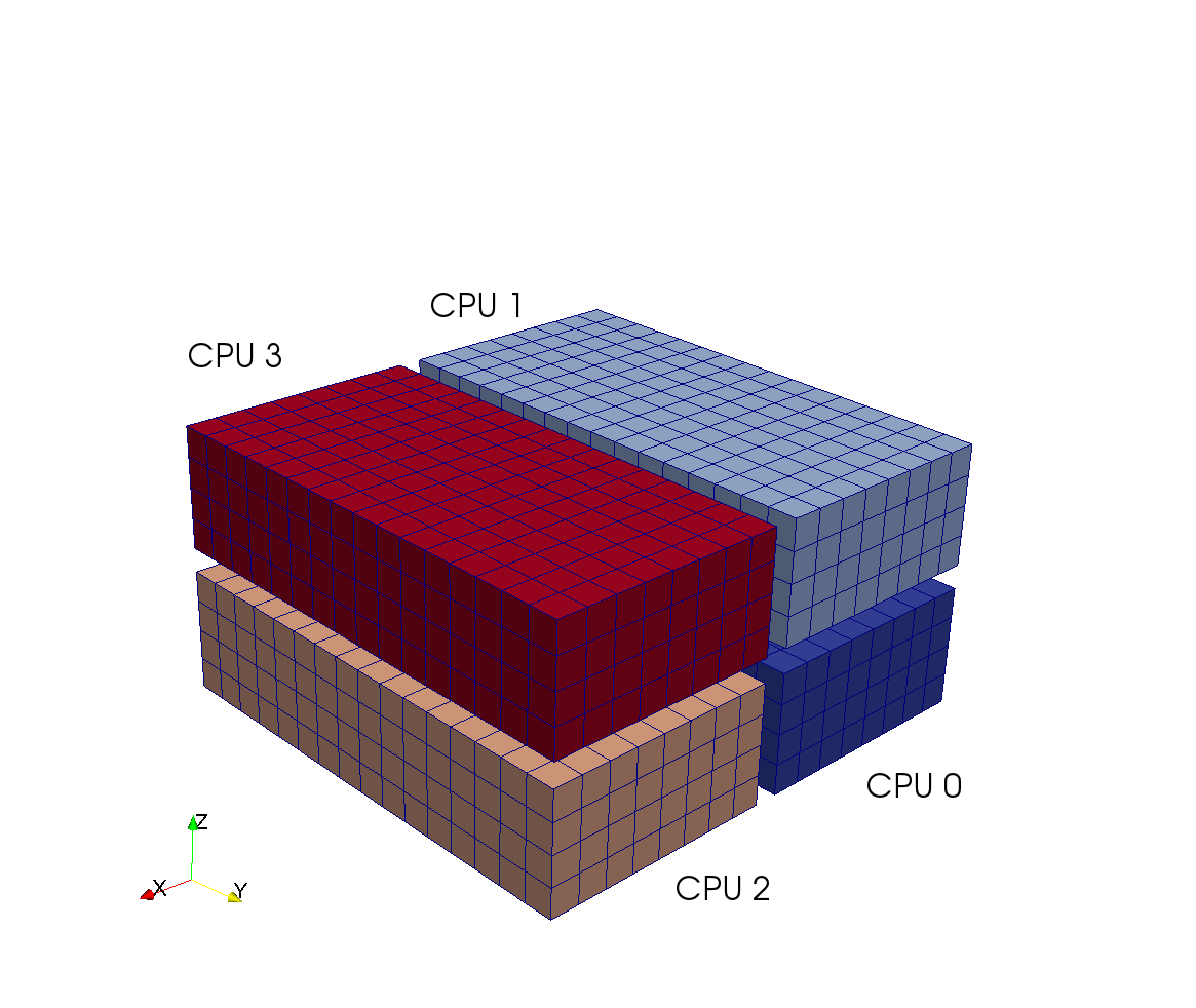
The 2D pencil decomposition strategy is illustrated in Figure 3 for a physical computational box of size $16^{3}$, using 4 CPUs. The datastructures are split in the plane normal to the direction in which the FFT is performed. That is, for the physical mesh in Figure 3 (a) the $x-y$ plane is split up in a $2\times 2$ processor mesh. Each CPU may now perform 64 ($=8\times 8$) real FFTs of length 16 in the $z$-direction on its own $8\times 8\times 16$ physical mesh. Afterwords, the complex data are laid out as shown in Figure 3 (b). The second transform takes place in the $x$-direction, and for this to happen, data must be exchanged between processors 0 and 1 as well as 2 and 3. The datastructures must also be transformed to the shape seen in Figure 3 (c). Each CPU may now perform the 32 ($4\times 8$) individual 1D FFTs in the $x$-direction. The same procedure is followed to end up with datastructures aligned in the final $y$-direction, see Figure 3 (d). However, this time processor 0 communicates with processor 2 and likewise 1 with 3. Evidently, each processor belongs to two different groups of communicators. One for communication in the $x-z$ plane (Figure 3 (b) to (c)) and one for communication in the $x-y$ plane (Figure 3 (c) to (d)). The MPI communicator groups and the distributed mesh are created in Python as shown in Figure 4

⬇

P2 = num_processes / P1 # CPUs in 2nd dir

N1 = N/P1

N2 = N/P2

# Create two communicator groups

commxz = comm.Split(rank/P1)

commxy = comm.Split(rank%P1)

# Get local ranks

xzrank = commxz.Get_rank()

xyrank = commxy.Get_rank()

# Create the decomposed physical mesh

x1 = slice(xzrank * N1, (xzrank+1) * N1)

x2 = slice(xyrank * N2, (xyrank+1) * N2)

X = mgrid[x1, x2, :N].astype(float)*L/N

# Create the decomposed wavenumber mesh

k2 = slice(xyrank*N2, (xyrank+1)*N2)

k1 = slice(xzrank*N1/2, (xzrank+1)*N1/2)

K = array(meshgrid(kx[k2], kx, kx[k1],

indexing=’ij’), dtype=int)

Figure 4: Creation of MPI communicator groups and physical and wavenumber meshes for pencil decomposition.

With reference to Figure 3, the two communicator groups for CPU with global rank 0 is commxz = [0, 1] and commxy = [0, 2]. The decomposition contains two parameters, P1 and P2, that are used to split up the first two indices of the physical mesh. For the case shown P1 may be either 1 or 2, in which case the second parameter P2 is 4 or 2 to arrive at a total of num_processes = P1*P2.

The entire 7 lines of code required for the Python implementation of the 3D parallel FFT with the 2D pencil decomposition appears in Figure 5. The work arrays Uc_hat_y, Uc_hat_x, Uc_hat_z are laid out as seen in Figure 3 (d), (c) and (b) respectively. The array Uc_hat_xr is a copy of Uc_hat_x used only for communication. Note that all MPI communications take place with the data aligned in the $x$-direction, as shown in Figure 3 (c), because this requires no preparation for the Alltoall call. The first index is automatically split up and distributed. In the call to Alltoall the first dimension of Uc_hat_x, i.e. $N$, is automatically broadcasted such that for commxz Uc_hat_x gets the shape (P1, N1, N2, N1/2) and commxy (P2, N2, N2, N1/2).

Note that the Nyquist frequency has been neglected for the pencil decomposition. This is not uncommon in turbulence simulations, because the Nyquist frequency ($k=N/2+1$) “is a coefficient for a Fourier mode that is not carried in the Fourier representation of the solution” [14]. Another more practical reason is that the number of independent wavenumbers in the z-direction is odd and thus not possible to share evenly between an even number of processors. There are, however, several different solutions to this problem, besides neglecting the Nyquist frequency. One solution is to let one processor have responsibility for one more wavenumber than the others, which leads to slightly poor load balancing (increasingly better for large number of processors). A better choice then is to place the real numbers of the Nyquist frequency in the complex part of the lowest wavenumber (which is also real) before transforming and communicating. This is done by Pekurovsky et al. [24] in their P3DFFT code. The approach is quite easily implemented in Python, taking no more than 10 extra lines of code for both the forward and the backward transforms. However, there is additional communication and the computational cost is slightly higher. For this reason, we have here simply chosen to neglect the Nyquist frequency.

⬇

"""fft in three directions using MPI and the pencil decomposition"""

Uc_hat_z[:] = rfft(u, axis=2)

# Transform to x direction neglecting k=N/2 (Nyquist)

Uc_hat_x[:] = rollaxis(Uc_hat_z[:,:,:-1].reshape((N1, N2, P1, N1)), 2). \

reshape(Uc_hat_x.shape)

# Communicate and do fft in x-direction

commxz.Alltoall([Uc_hat_x, mpitype], [Uc_hat_xr, mpitype])

Uc_hat_x[:] = fft(Uc_hat_xr, axis=0)

# Communicate and transform to z-direction

commxy.Alltoall([Uc_hat_x, mpitype], [Uc_hat_xr, mpitype])

Uc_hat_y[:] = rollaxis(Uc_hat_xr.reshape((P2, N2, N2, N1)), 1). \

reshape(Uc_hat_y.shape)

fu[:] = fft(Uc_hat_y, axis=1)

return fu

Figure 5: Three dimensional forward fftn_mpi FFT implemented for the pencil decomposition.

3.4 Optimization

The scientific Python implementation discussed thus far is using no more than NumPy and MPI for Python, and possibly pyFFTW for faster FFTs. The FFTs represent the major computational cost of the solver, but there is also significant cost in all the elementwise operations on the structured NumPy arrays required to build the right hand side of the Navier-Stokes equations ( see the computeRHS function). The elementwise operations, like multiply and divide, are handled by NumPy’s universal functions (ufuncs), that are fast because they are implemented in C. However, some of the ufuncs may be inefficient due to temporary arrays that need to be created, especially for multiple-operator expressions. The most glaring example for the current solver is the cross product (used in computing convection, see Eq. (17)), which is computed most straightforward though NumPy as

⬇

"""c = a x b"""

#Alternative numpy cross product:

#c = numpy.cross(a, b, axis=0)

c[0] = a[1]*b[2]-a[2]*b[1]

c[1] = a[2]*b[0]-a[0]*b[2]

c[2] = a[0]*b[1]-a[1]*b[0]

return c

Note that we have commented out the use of NumPy’s cross function, which is implemented under the hood using ufuncs and runs at approximately the same computational speed as the alternative shown. The term a[1]*b[2]-a[2]*b[1] requires two elementwise multiplications and one elementwise subtraction. This is implemented by NumPy using three separate ufuncs (two multiply, one subtract), each with temporary arrays allocated. For the three items in the c vector, this means that 9 ufuncs are called and the loop over all $N^{3}$ indices in the mesh is performed 9 times, which, needless to say, is very inefficient even though it is vectorized.

For straightforward comparison, the Python solver with slab decomposition has been used as prototype for a pure C++ implementation. The only significant difference between the solvers is that for C++, the 3D FFT computations are using the MPI communication routines that are provided directly through the FFTW library. Otherwise, everything is exactly the same. For a first direct comparison, though, we are neglecting the MPI implementation and running the Python and C++ codes in serial for the Taylor Green test case (see Section 4.2) for three meshes of size $(32^{3},64^{3},128^{3})$. On a MacBook Pro with 2.8 GHz Intel Core i7 we find that the C++ code runs at (0.0092, 0.083, 0.80) seconds per time step for the three mesh sizes, whereas the pure Python solver runs at (0.013, 0.12, 1.3) seconds. As such we may conclude that without MPI the C++ code is approximately 30 % faster. Considering the issue recently discussed with the cross product, we are all in all quite happy with the performance of the Python solver.

Fortunately, many different strategies are known for speeding up pure NumPy code, e.g., Numba [19], Numexpr [20], Weave [31] and Cython [6]. We have obtained best results for Numba and Cython. The Numba module uses just in time compilation of Python functions chosen for optimization. The advantage of using Numba is that no compilation or installation is required by the user who never has to leave the pure Python environment. The downside is that Numba is difficult to install on non-standard platforms like the Blue Gene/P. Nevertheless, a Numba optimized cross product routine may be implemented in an external module and code will be generated and compiled when this module is imported. For efficient speed-up on our structured mesh the code must be rewritten using explicit for loops as seen in Figure 6. The Numba cross product may now be used directly in place of the pure Python version with no further modifications.

⬇

@jit(float[:,:,:,:](float[:,:,:,:],

float[:,:,:,:], float[:,:,:,:]))

def cross(a, b, c):

for i in xrange(a.shape[1]):

for j in xrange(a.shape[2]):

for k in xrange(a.shape[3]):

a0 = a[0,i,j,k]

a1 = a[1,i,j,k]

a2 = a[2,i,j,k]

b0 = b[0,i,j,k]

b1 = b[1,i,j,k]

b2 = b[2,i,j,k]

c[0,i,j,k] = a1*b2 - a2*b1

c[1,i,j,k] = a2*b0 - a0*b2

c[2,i,j,k] = a0*b1 - a1*b0

return c

Figure 6: Numba implementation of the cross product in double precision.

Cython has gained much momentum in recent years and is usually the obvious choice for high performance computing. Using Cython, the cross product should be implemented like for Numba, through explicit for loops which are translated to efficient C code to be highly optimized by the compiler. As shown in Figure 7 an external module may be created and compiled using Python’s standard installation utilities (distutils).

⬇

#cython: wraparound=False

cimport numpy as np

ctypedef np.float64_t real_t

def cross(np.ndarray[real_t, ndim=4] a,

np.ndarray[real_t, ndim=4] b,

np.ndarray[real_t, ndim=4] c):

cdef unsigned int i, j, k

cdef real_t a0, a1, a2, b0, b1, b2

for i in xrange(a.shape[1]):

for j in xrange(a.shape[2]):

for k in xrange(a.shape[3]):

a0 = a[0,i,j,k]

a1 = a[1,i,j,k]

a2 = a[2,i,j,k]

b0 = b[0,i,j,k]

b1 = b[1,i,j,k]

b2 = b[2,i,j,k]

c[0,i,j,k] = a1*b2 - a2*b1

c[1,i,j,k] = a2*b0 - a0*b2

c[2,i,j,k] = a0*b1 - a1*b0

Figure 7: Cython implementation of the cross product in double precision.

Cython generated modules may be imported into Python and the cross function from Cython may be used directly in place of the pure Python version. The Cython code for the cross product runs at about the same speed as Numba and approximately 3 times faster than pure NumPy for a mesh of size $128^{3}$. When Cython is used to compute all elementwise operations that generate the right hand side of the Navier-Stokes equations, the Taylor Green test case runs at (0.0090, 0.080, 0.82) seconds per time step. In other words, with a few quick Cython wrappers we have a Python solver that is comparable in speed to its low-level counterpart in C++. And this solver is scripted and operated in a comfortable interactive environment where post processing and plotting may be performed from a commandline shell.

4 Parallel performance

Our scientific Python DNS solver has been tested on the Shaheen computer at the KAUST Supercomputing Laboratory. The primary computational resource of Shaheen consists of 16 racks of Blue Gene/P. Each rack contains 1024 quad-core, 32-bit, 850 MHz PowerPC compute nodes, for a total of 65,536 compute cores. Each node is equipped with 4GB of system memory, providing a total 64TB of distributed memory across the resource. Blue Gene nodes are interconnected by a three-dimensional point-to-point “torus” network used for general-purpose message-passing and multicast communication.

4.1 Dynamic loading of Python

Running a Python solver on a supercomputer presents a few challenges. Most importantly, the dynamic loading time of Python, i.e., the time to simply get started, may become unreasonably high. To load Python with NumPy on the complete 16 racks of Shaheen takes approximately 45 minutes. The main reason is that large-scale supercomputers, such as Shaheen, make use of parallel file systems designed to support large distributed loads, where each CPU is writing or reading data independently. With dynamic loading, however, each process attempts to access the same files simultaneously and bottlenecks appear.

A few solutions to the loading problem are known. The MPI_Import Python module of Langton [13] is designed to overload the built in import mechanism of Python such that only one rank (the zero rank) searches the filesystem for a module and then subsequently broadcasts the results to the remaining ranks. A drawback is the Python implementation where several modules (e.g., sys, imp, __builtin__,types, mpi4py) need to be imported through the regular Python import mechanism. A second approach of Langton is to rewrite the regular finders and loaders modules such that one rank does all the initial work, caching the modules it finds.

A better solution is provided through the Scalable Python implementation [27, 9], used, e.g., by GPAW [16]. Here CPython is modified slightly such that during import operations only a single process performs the actual I/O, and MPI is used for broadcasting the data to other MPI ranks. The solution provided by Scalable Python is used in this work and as such dynamic loading times are kept very low (approximately 30 seconds for a full rack).

4.2 Verification

To verify the implementation of the scientific Python DNS solver we run the Taylor Green test case for a Reynolds number of 1600. This is a well known test case used, e.g., by the annual Workshop on High-Order CFD Methods, which provides reference data for the temporal evolution of kinetic energy, energy dissipation and vorticity integrated over the computational domain. The Taylor Green test case at Re=1600 starts out as laminar with only one single length scale, and then through a series of complex flow patterns a fully developed, decaying, turbulent flow is obtained. The Taylor Green vortex is initialized as

⬇

dt = 0.001

U[0] = sin(X[0])*cos(X[1])*cos(X[2])

U[1] =-cos(X[0])*sin(X[1])*cos(X[2])

U[2] = 0

for i in range(3):

U_hat[i] = fftn_mpi(U[i], U_hat[i])

where the same code is used for both the slab and the pencil decomposition. The Reynolds number is fixed at 1600 by setting the viscosity coefficient to 1/1600 and the time step is fixed at 0.001. We use a real mesh of size $N=512$, since that matches the reference data. A resolution of $512^{3}$ is reported by by Bratchet [3] to represent a fully resolved DNS of this flow.

The non-optimized code is run on Shaheen using the pencil decomposition and 2048 cores. The entire simulation is set for 20 seconds real time, during which the flow undergoes transition, decays and finally fades out. The simulation takes 12 hours alltogether ($12\cdot 2048$ CPU hours) and neither the kinetic energy nor the vorticity stray more than 0.01 % from the reference solutions, even after 20,000 time steps.

4.3 Parallel scaling

In this section we will investigate parallel scaling and performance of the solver described in previous sections. Optimization of the scientific Python solver will be based on Cython and not Numba, because we only managed to install the former on the Blue Gene nodes. We compare our Python based solvers to the C++ solver described briefly in Sec 3.4 and note that the C++ solver is using the same compiled FFTW library as the Python code. However, it is also important to note that the Python code only makes use of the serial versions of the FFTW routines and performs the MPI communications itself through MPI fo Python, whereas the C++ code uses the built in MPI communication routines that come with the FFTW library.

The only MPI communication required by the current solver can be found in the 3D FFT routines, or when global results, like the total kinetic energy, are computed. Scaling will be efficient as long as the cost for MPI communication is smaller than all the other elementwise operations required to set up the right hand side of the explicit ODE given by Eq. (14). This is not a trivial task, considering that a pseudo-spectral solver demands that every process sends and receives data from all the other processes - at least for the slab decomposition.

It is customary for pseudo-spectral solvers to assume that the main computational cost is due to Fourier transforms, and as such the CPU time should ideally scale like

$$\frac{N^{3}\log_{2}N}{M},$$ (18)

where $M$ is the number of CPUs. In other words, strong scaling implies, as usual, CPU time per time step proportional to $1/M$, whereas weak scaling, where $N^{3}/M$ is kept constant, should ideally show CPU times proportional to $\log_{2}N$. A more thorough analysis of scalability factors for a 3D FFT using the pencil domain decomposition has been given by Ayala and Wang [1]. Note that all results are computed using single precision arithmetics, which is customary for scaling tests of similar DNS solvers.

4.3.1 Weak scaling

Since MPI communications are primarily required by the FFTs, we first run a weak scaling test of the pure forward and inverse FFTs before proceeding to the complete solver. To this end we keep the ratio of mesh size to number of processors ($N^{3}/M$) constant, which ideally should lead to CPU times proportional to $\log_{2}N$. Both slab and pencil decompositions are tested using four meshes of size $N^{3}$, where $N=(2^{7},2^{8},2^{9},2^{10})=(128,256,512,1024)$. For these meshes the slab decomposition uses $M=(2,16,128,1024)$ number of CPUs and the pencil uses twice as many $M=(4,32,256,2048)$ with $P1=(2,4,16,32)$. Note that for $N=1024$ the maximum number of CPUs is reached for the slab decomposition, whereas the pencil decomposition may still use many more. The performance of the FFTs is compared to a C++ code using the same FFTW library with plans corresponding to the Python solver. A simplified setup that also shows how the code is executed is shown in Figure 8. The FFTW library is using a slab mesh decomposition.

⬇

typedef float precision;

int N = pow(static_cast<int>(2), 9);

ptrdiff_t alloc_local, local_n0, local_0_start, local_n1, local_1_start

fftwf_plan rfftn, irfftn;

alloc_local = fftw_mpi_local_size_3d_transposed(N, N, N/2+1,

MPI::COMM_WORLD, &local_n0, &local_0_start,

&local_n1, &local_1_start);

vector<precision> U(2*alloc_local);

vector<complex<precision> > U_hat(alloc_local);

rfftn = fftwf_mpi_plan_dft_r2c_3d(N, N, N, U.data(),

reinterpret_cast<fftwf_complex*>(U_hat.data()),

MPI::COMM_WORLD, FFTW_MPI_TRANSPOSED_OUT);

irfftn = fftwf_mpi_plan_dft_c2r_3d(N, N, N,

reinterpret_cast<fftwf_complex*>(U_hat.data()),

U.data(), MPI::COMM_WORLD, FFTW_MPI_TRANSPOSED_IN);

// Execute forward and inverse transforms

fftwf_mpi_execute_dft_r2c( rfftn, U.data(),

reinterpret_cast<fftwf_complex*>(U_hat.data()));

fftwf_mpi_execute_dft_c2r(irfftn,

reinterpret_cast<fftwf_complex*>(U_hat.data()), U.data());

// Scale the inverse FFT

for (int k=0; k<U.size(); k++)

U[k] /= tot;

Figure 8: C++ setup for the parallel FFT using FFTW.

Figure 9: Weak scaling of forward and inverse FFTs. The scientific Python results are not optimized and C++ is using slab decomposition with MPI communication performed through the FFTW library. The pencil timings are scaled by a factor 0.5 since the pencil results are collected using twice as many cores as slab.

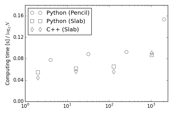
The results are collected as the fastest of 10 forward and inverse FFTs (only execution time, not the setup), and the timings are scaled by $\log_{2}N$ and plotted in Figure 9. Perfect scaling would thus imply a constant compute time as the number of cores is increased. From Figure 9 we observe that both slab and pencil versions of the Python 3D FFTs show good scaling, and only start to trail off significantly for the largest mesh size. The C++ routine can be seen to be slightly faster than Python (slab) for the smallest number of processors (64), whereas the Python routine is fastest for the largest number of cores (1024). In other words, the Python 4-liners (see Figure 1) that embody the complete execution of the 3D FFT with MPI scales slightly better than the 3D FFT routines with MPI provided by FFTW.

From Figure 9 we also observe that the slab decomposition is more efficient than pencil, which is generally in agreement with previous studies (see, e.g., [24]). Note that the pencil computations are using twice as many cores for the same mesh as the slab computations. As such the pencil results in Figure 9 have been scaled by a factor 0.5 to allow for a direct comparison.

Turning now to the complete solver, we run the Taylor Green test case for 100 time steps on the same meshes that were used for the weak scaling of the FFTs. Figure 10 shows the computing times for one such time step (the fastest) for both the scientific Python solver 10(a) and the version optimized with Cython 10(b). The figures clearly show how the Cython optimization leads to a solver that performs as well as C++ for the entire range of processors. Both the slab and pencil optimized implementations are seen to be approximately $20\%$ faster than their non-optimized Python counterparts, but there is generally no difference in scaling performance. Like for the pure FFT test, the scaling performance of the Python solver is actually slightly better than C++, and this leads to the optimized Python solver actually being the fastest for 1024 processors.

(a) Scientific Python solver

(b) Python solver optimized with Cython

Figure 10: Weak scaling of DNS solver. The slab decompositions are using $4\cdot 64^{3}$ nodes per core, whereas the pencil decomposition uses $2\cdot 64^{3}$. The C++ solver uses slab decomposition with MPI communication performed through the FFTW library. The C++ results are the same in 10(a) and 10(b).

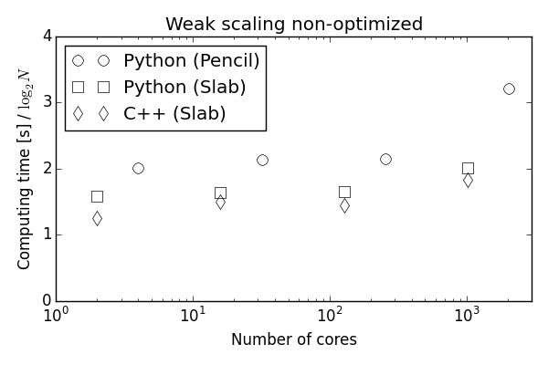
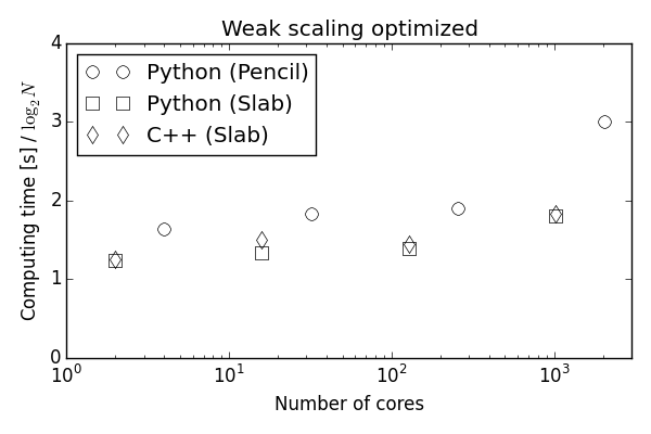
4.3.2 Strong scaling

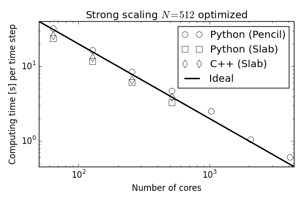
Strong scaling over a wide range of processors is usually more challenging to prove than weak, in our case partly because the efficiency of the FFT routines depends on the length of the datastructures and how well they fit into memory. Nevertheless, we have performed strong scaling tests of the FFTs and the complete solvers using a computational box of size $512^{3}$.

Figure 11: Strong scaling of forward and inverse FFTs. The Python results are non-optimized and C++ is using slab decomposition with MPI communication performed through the FFTW library.

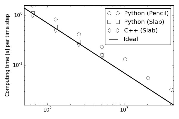
Isolating first the FFTs we plot in Figure 11 the computing time of one forward and inverse FFT, for both the pencil and slab decompositions and, as for the weak scaling, compare it to a C++ version that is using FFTW. The number of cores is varied over the range from 64 to 512 for the slab decomposition, and from 64 to 4096 for the pencil decomposition. The scaling is very good for both slab and pencil, and good speedup is observed throughout the entire range. Like for the weak scaling, the Python slab version is seen also here to scale better than the C++ version for the highest number of processors, and even though C++ is approximately 10 % faster for 64 processors, the Python version is actually faster for 512. The pencil transforms are again seen to be slower than slab, but we achieve good, although not perfect, speedup all the way up to 4096 processors. Note that the results for the pencil transforms depend on the parameter P1, fixed to determine how the two first indices of the computational mesh are distributed. Here we have used $P1=(8,16,16,32,32,64,64)$ and not optimized any further.

Figure 12 shows the performance of the complete solvers. The outcome is similar to that found in the weak scaling test and the optimized Python/Cython code is seen to more than match the performance of the C++ solver for this particular case. Good scaling is observed for the pencil solver all the way up to 4096 processors.

(a) Scientific Python solver

(b) Python solver optimized with Cython

Figure 12: Strong scaling of the DNS solver. The C++ solver uses slab decomposition with MPI communication performed through the FFTW library. The C++ results are the same in 12(a) and 12(b).

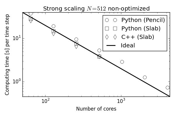
4.4 Comparison to Tarang

At this point the reader may still be skeptical since the C++ solver described in previous sections is not a properly tested and optimized code, and therefore the comparison may not seem fair. For this reason we will finally comment on the performance in relation to the open source C++ pseudo-spectral solver Tarang [30]. Tarang is using the same 4’th order Runge-Kutta integrator as our code, dealiasing is performed in the same way and 3D FFT is performed using FFTW with slab decomposition. As such, computational cost should be more or less identical and the computational speed should be directly comparable to our solver. Furthermore, Tarang has been benchmarked by its own developers on Shaheen.

With this in mind we can collect the timings from Figure 2 of [30], which reads that a box of size $1024^{3}$ (single precision) is running at approximately $50$ seconds per time step, and that a perfectly scaled solver would optimally run at approximately 32 seconds. From the largest mesh used in Figure 10 b) results are plotted for a box of size $1024^{3}$ using 1024 cores. The actual timing reads approximately 18 seconds, whereas optimal performance (perfect weak scaling) would be achieved at slightly less than 15 s. Assuming perfect strong scaling down to 512 cores, this would correspond to 36/30 seconds for actual and optimal performance on the same mesh as used by Tarang. Comparing to Tarang, the optimal performance is thus found to be very similar, whereas the actual is nearly 30 % faster due to better scaling. This leads us to suspect that Tarang has not been using an optimal installation of FFTW on Shaheen, because our C++ solver (which is also using FFTW for parallel FFT), is scaling much better, and scaling performance depends almost exclusively on the 3D parallel FFT.

5 Conclusions

We have described a parallel Python implementation of an open source pseudo-spectral DNS solver for turbulent flows. The solver is implemented using standard scientific Python modules (NumPy, MPI for Python) and a very high level of abstraction, using no more than 100 lines of code, just like a similar MATLAB script, but targeting supercomputer platforms. We have then discussed an optimization of a small part of this solver through the use of Cython. The solver has been verified and benchmarked on the Shaheen supercomputer at the KAUST supercomputing laboratory, and we are able to show excellent scaling up to several thousand cores with performance matching that of a pure C++ implementation.

Appendix

In this Appendix we show a complete Python script that solves Eq. (14) with slab decomposition and a fourth order Runge Kutta method for the Taylor Green test case. Saved as TG.py it runs in parallel on 128 processors with command mpirun -np 128 python TG.py.

⬇

1from numpy.fft import fftfreq, fft, ifft, irfft2, rfft2

2from mpi4py import MPI

3

4nu = 0.000625

5T = 0.1

6dt = 0.01

7N = 2**7

8comm = MPI.COMM_WORLD

9num_processes = comm.Get_size()

10rank = comm.Get_rank()

11Np = N / num_processes

12X = mgrid[rank*Np:(rank+1)*Np, :N, :N].astype(float)*2*pi/N

13U = empty((3, Np, N, N))

14U_hat = empty((3, N, Np, N/2+1), dtype=complex)

15P = empty((Np, N, N))

16P_hat = empty((N, Np, N/2+1), dtype=complex)

17U_hat0 = empty((3, N, Np, N/2+1), dtype=complex)

18U_hat1 = empty((3, N, Np, N/2+1), dtype=complex)

19dU = empty((3, N, Np, N/2+1), dtype=complex)

20Uc_hat = empty((N, Np, N/2+1), dtype=complex)

21Uc_hatT = empty((Np, N, N/2+1), dtype=complex)

22U_mpi = empty((num_processes, Np, Np, N/2+1), dtype=complex)

23curl = empty((3, Np, N, N))

24kx = fftfreq(N, 1./N)

25kz = kx[:(N/2+1)].copy(); kz[-1] *= -1

26K = array(meshgrid(kx, kx[rank*Np:(rank+1)*Np], kz, indexing=’ij’), dtype=int)

27K2 = sum(K*K, 0, dtype=int)

28K_over_K2 = K.astype(float) / where(K2 == 0, 1, K2).astype(float)

29kmax_dealias = 2./3.*(N/2+1)

30dealias = array((abs(K[0]) < kmax_dealias)*(abs(K[1]) < kmax_dealias)*

31 (abs(K[2]) < kmax_dealias), dtype=bool)

32a = [1./6., 1./3., 1./3., 1./6.]

33b = [0.5, 0.5, 1.]

34

35def ifftn_mpi(fu, u):

36 Uc_hat[:] = ifft(fu, axis=0)

37 comm.Alltoall([Uc_hat, MPI.DOUBLE_COMPLEX], [U_mpi, MPI.DOUBLE_COMPLEX])

38 Uc_hatT[:] = rollaxis(U_mpi, 1).reshape(Uc_hatT.shape)

39 u[:] = irfft2(Uc_hatT, axes=(1, 2))

40 return u

41

42def fftn_mpi(u, fu):

43 Uc_hatT[:] = rfft2(u, axes=(1,2))

44 U_mpi[:] = rollaxis(Uc_hatT.reshape(Np, num_processes, Np, N/2+1), 1)

45 comm.Alltoall([U_mpi, MPI.DOUBLE_COMPLEX], [fu, MPI.DOUBLE_COMPLEX])

46 fu[:] = fft(fu, axis=0)

47 return fu

48

49def Cross(a, b, c):

50 c[0] = fftn_mpi(a[1]*b[2]-a[2]*b[1], c[0])

51 c[1] = fftn_mpi(a[2]*b[0]-a[0]*b[2], c[1])

52 c[2] = fftn_mpi(a[0]*b[1]-a[1]*b[0], c[2])

53 return c

54

55def Curl(a, c):

56 c[2] = ifftn_mpi(1j*(K[0]*a[1]-K[1]*a[0]), c[2])

57 c[1] = ifftn_mpi(1j*(K[2]*a[0]-K[0]*a[2]), c[1])

58 c[0] = ifftn_mpi(1j*(K[1]*a[2]-K[2]*a[1]), c[0])

59 return c

60

61def computeRHS(dU, rk):

62 if rk > 0:

63 for i in range(3):

64 U[i] = ifftn_mpi(U_hat[i], U[i])

65 curl[:] = Curl(U_hat, curl)

66 dU = Cross(U, curl, dU)

67 dU *= dealias

68 P_hat[:] = sum(dU*K_over_K2, 0, out=P_hat)

69 dU -= P_hat*K

70 dU -= nu*K2*U_hat

71 return dU

72

73U[0] = sin(X[0])*cos(X[1])*cos(X[2])

74U[1] =-cos(X[0])*sin(X[1])*cos(X[2])

75U[2] = 0

76for i in range(3):

77U_hat[i] = fftn_mpi(U[i], U_hat[i])

78

79t = 0.0

80tstep = 0

81while t < T-1e-8:

82 t += dt; tstep += 1

83 U_hat1[:] = U_hat0[:] = U_hat

84 for rk in range(4):

85 dU = computeRHS(dU, rk)

86 if rk < 3: U_hat[:] = U_hat0 + b[rk]*dt*dU

87 U_hat1[:] += a[rk]*dt*dU

88 U_hat[:] = U_hat1[:]

89 for i in range(3):

90 U[i] = ifftn_mpi(U_hat[i], U[i])

91

92k = comm.reduce(0.5*sum(U*U)*(1./N)**3)

93if rank == 0:

94 assert round(k - 0.124953117517, 7) == 0

References

- [1] O. Ayala and L. P. Wang. Parallel implementation and scalability analysis of 3D Fast Fourier Transform using 2D domain decomposition. Parallel Computing, 39:58–77, 2013.
- [2] S. Balay, J. Brown, K. Buschelman, W. D. Gropp, D. Kaushik, M. G. Knepley, L. Curfman McInnes, B. F. Smith, and H. Zhang. PETSc Web page. http://www.mcs.anl.gov/petsc.
- [3] M. E. Brachet. Direct simulation of three-dimensional turbulence in the taylor-green vortex. Fluid dynamics research, 8(1):1–8, 1991.
- [4] C. Canuto, M. Y. Hussaini, A. Quarteroni, and T. A. Zang. Spectral Methods in Fluid Dynamics. Springer-Verlag New York-Heidelberg-Berlin, 1988.
- [5] S. G. Chumakov. https://code.google.com/p/hit3d/.
- [6] Cython. http://cython.org.
- [7] S. de Bruyn Kops. Classical scaling and intermittency in strongly stratified boussinesq turbulence. J. Fluid Mechanics, 775:436–463, 2015.
- [8] H. Q. Ding, R. D. Ferraro, and D. B. Gennery. A portable 3D FFT package for distributed-memory parallel architectures. In Proceedings of 7th SIAM Conference on Parallel Processing, pages 70–71, 1995.
- [9] J. Enkovaara, N. A. Romero, S. Shende, and J. J. Mortensen. GPAW - massively parallel electronic structure calculations with python-based software. Procedia Computer Science, 4(0):17 – 25, 2011.
- [10] FEniCS. http://fenicsproject.org.
- [11] M. Iovieno et. al. http://areeweb.polito.it/ricerca/ philofluid/.
- [12] D. Ketcheson, K. Mandli, A. Ahmadia, A. Alghamdi, M. de Luna, M. Parsani, M. Knepley, and M. Emmett. Pyclaw: Accessible, extensible, scalable tools for wave propagation problems. SIAM Journal on Scientific Computing, 34(4):C210–C231, 2012.
- [13] A. Langton. https://github.com/langton/MPIImport.
- [14] M. Lee, N. Malaya, and R. D. Moser. Petascale direct numerical simulation of turbulent channel flow on up to 786k cores. In Proceedings of the International Conference on High Performance Computing, Networking, Storage and Analysis, pages 61:1–61:11, New York, USA, 2013.
- [15] N. Li and S. Laizet. 2DECOMP&FFT - A highly scalable 2D decomposition library and FFT interface. In Cray User Group conference, Edinburgh. 2010.
- [16] J. J. Mortensen, L. B. Hansen, and K. W. Jacobsen. Real-space grid implementation of the projector augmented wave method. Phys. Rev. B, 71(3):035109, 2005.
- [17] M. Mortensen and K. Valen-Sendstad. Oasis: A high-level/high-performance open source Navier - Stokes solver. Computer Physics Communications, 188(0):177 – 188, 2015.
- [18] MPI for Python. https://bitbucket.org/mpi4py/mpi4py/.
- [19] Numba. http://numba.pydata.org.
- [20] Numexpr. http://github.com/pydata/numexpr.
- [21] NumPy. http://www.numpy.org.
- [22] S. A. Orzag. On the Elimination of Aliasing in Finite Difference Schemes by Filtering High-Wavenumber Components. Journal of the Atmospheric Sciences, 28:1074, 1971.
- [23] D. Pekurovsky. P3DFFT http://code.google.com/p/ p3dfft/.
- [24] D. Pekurovsky. P3DFFT: a framework for parallel computations of Fourier transforms in three dimensions. SIAM Journal on Scientific Computing, 34(4), 2012.
- [25] M. Pippig. PFFT - An extension of FFTW to massively parallel architectures. SIAM J. Sci. Comput., 35:C213 – C236, 2013.
- [26] S. J. Plimpton. Parallel FFT Subroutine Library http://www.sandia.gov/sjplimp/docs/fft/ README.html.
- [27] Scalable Python. https://github.com/CSC-IT-Center-for-Science/scalable-python.
- [28] B. Teaca. http://aqua.ulb.ac.be/home/turbo/.
- [29] Stefan Van Der Walt, S Chris Colbert, and Gael Varoquaux. The NumPy array: a structure for efficient numerical computation. Computing in Science & Engineering, 13(2):22–30, 2011.
- [30] M. Vermi. http://turbulence.phy.iitk.ac.in/doku.php.
- [31] Weave. http://docs.scipy.org/doc/scipy/reference/ tutorial/weave.html.