On the validity of power functionals for the homogeneous electron gas
in reduced-density-matrix-functional theory

Abstract

Physically valid and numerically efficient approximations for the exchange and correlation energy are critical for reduced-density-matrix-functional theory to become a widely used method in electronic structure calculations. Here we examine the physical limits of power functionals of the form $f(n,n^{\prime})=(nn^{\prime})^{\alpha}$ for the scaling function in the exchange-correlation energy. To this end we obtain numerically the minimizing momentum distributions for the three- and two-dimensional homogeneous electron gas, respectively. In particular, we examine the limiting values for the power $\alpha$ to yield physically sound solutions that satisfy the Lieb-Oxford lower bound for the exchange-correlation energy and exclude pinned states with the condition $n({\bf k})<1$ for all wave vectors ${\bf k}$. The results refine the constraints previously obtained from trial momentum distributions. We also compute the values for $\alpha$ that yield the exact correlation energy and its kinetic part for both the three- and two-dimensional electron gas. In both systems, narrow regimes of validity and accuracy are found at $\alpha\gtrsim 0.6$ and at $r_{s}\gtrsim 10$ for the density parameter, corresponding to relatively low densities.

I Introduction

Reduced-density-matrix-functional theory lowdin ; gilbert (RDMFT) has attracted interest and popularity as an alternative to density-functional theory dft (DFT) to deal with complicated many-particle problems. In contrast with the one-body density in DFT, the key quantity in RDMFT is the one-body reduced density matrix (1-RDM), which provides the exact kinetic energy. It is thus evident that RDMFT can outperform DFT in strongly correlated systems corre1 ; corre2 ; corre3 , and recent extensions and investigations include, e.g., finite temperatures finitetemp , excitation energies excitations , and Mott insulators mott1 ; mott2 . However, so far only a few energy functionals of the 1-RDM have been developed, and their practical applicability is still partly unknown.

The so-called power functionals sharma of RDMFT have been applied in three-dimensional (3D) systems during the past few years nek1 ; nek2 ; mott2 . In this functional the scaling factor for the exchange-correlation ($xc$) energy $E_{xc}$ has a form $f(n,n^{\prime})=(nn^{\prime})^{\alpha}$, where $1/2\leq\alpha\leq 1$ can be viewed as a parameter interpolating between the Hartree-Fock (HF) ($\alpha=1$) and Müller muller ($\alpha=0.5$) approximations. The optimal values for $\alpha$ have been found to vary between $0.525$ (stretched $H_{2}$) and $0.65$ (solids). The best overall fit for the 3D homogeneous electron gas (3DEG) has been obtained with $\alpha=0.55\ldots 0.58$ nek2 . In the two-dimensional (2D) framework, the applications are more scarce. However, Harju and Tölö harju have found reasonable results for 2D quantum Hall droplets at high magnetic fields with $\alpha\sim 0.65\ldots 0.7$.

Power functionals are also subject to physical constraints of RDMFT levy . In the case of the 3DEG, strict constraints regarding the solution of the Euler-Lagrange equation and the Lieb-Oxford (LO) bound lo have been studied by Cioslowski and Pernal kasia ; kasia2 . A similar study on the 2D homogeneous electron gas (2DEG) has been recently carried out by some of the present authors with a particular attention on accessible densities antti . However, both of these studies have resorted to analysis of trial momentum distributions with uncertainty of their accuracy in comparison with numerically exact results.

In this work we numerically obtain the minimizing momentum distributions for the power functional in both the 3DEG and 2DEG. The resulting range of validity for $\alpha$ at various densities is then compared to the results obtained previously with trial momentum distributions in 3D kasia and 2D antti , respectively. In both cases we begin with the general constraints on $n({\bf k})$ and on the densities $\rho$. We then proceed with a closer analysis of (i) the LO bound lo with its recently suggested tighter forms ourbound , and (ii) the exclusion of pinned states with $n({\bf k})=1$ kimball ; klaas1 .

We find that in both 3D and 2D the power functionals have a rather limited range of validity, and only for relatively low densities, although the numerical solutions extend the range in comparison with the previously used trial momentum distributions. We also calculate numerically the exact correlation energies and their kinetic contributions as a function of $\alpha$. The exact solutions coincide only partly, if at all, with the regimes of validity.

II Homogeneous electron gas

For the homogeneous electron gas (EG), here generally in 3D or 2D, we can consider a positive background charge compensating for the electrostatic (Hartree) energy, so that the total energy consists of the kinetic and xc components alone, i.e.,

$$E^{\rm EG}_{\rm tot}[\gamma]=T[\gamma]+E_{xc}[\gamma].$$ (1)

In RDMFT, we can express the kinetic and xc energies (in Hartree atomic units) as

$$T[\gamma]=-\frac{1}{2}\sum_{\sigma=\uparrow,\downarrow}\sum_{p}n_{\sigma}({\bf k}_{p})\int d{\bf r}\,\varphi^{*}_{p\sigma}({\bf r})\nabla^{2}\varphi_{p\sigma}({\bf r})$$ (2)

and

$$E_{xc}[\gamma] = -\frac{1}{2}\sum_{\sigma=\uparrow,\downarrow}\sum_{p,q}^{\infty}\int d{\bf r}\int d{\bf r}^{\prime}f\left(n_{\sigma}({\bf k}_{p}),n_{\sigma}({\bf k}_{q})\right)$$ (3)

$$\times \frac{\varphi^{*}_{p\sigma}({\bf r})\varphi^{*}_{q\sigma}({\bf r}^{\prime})\varphi_{q\sigma}({\bf r})\varphi_{p\sigma}({\bf r}^{\prime})}{|{\bf r}-{\bf r}^{\prime}|}.$$

Here ${\bf k}_{p}$ is the wave vector of the $p$th spin-dependent natural orbital, which is a plane wave. Now, in the thermodynamic limit the summation over plane waves is placed by a momentum-space integration and, hence, we can express the total energy as a functional of the momentum distribution kasia ; antti . Using the normalization constraint and the variational Euler-Lagrange equation finally leads to

$$\frac{1}{2}|{\bf k}|^{2}-\frac{1}{2\pi^{d-1}}\int d{\bf k}^{\prime}\,\frac{\frac{\partial}{\partial n({\bf k})}f\left(n({\bf k}),n({\bf k}^{\prime})\right)}{|{\bf k}-{\bf k}^{\prime}|^{d-1}}=\mu,$$ (4)

where $\mu$ is the Lagrange multiplier, and $d=3$ in 3D and $d=2$ in 2D. Note that the spin index $\sigma$ has been omitted here, and in the following we consistently refer to quantities per particle with spin $\sigma$. It is important to appreciate that the Euler-Lagrange equation only holds for all ${\bf k}$ if the minimizing momentum distribution has no pinned states, i.e., $n({\bf k})\neq 1$ and $n({\bf k})\neq 0$ for all wave vectors ${\bf k}$.

The key quantity in the expressions above is the function $f\left(n({\bf k}),n({\bf k}^{\prime})\right)$ used in RDMFT as a scaling factor to take into account electron–electron correlations beyond the mean-field or HF level. Our main focus here is on the generic power functional,

$$f\left(n({\bf k}),n({\bf k}^{\prime})\right)=\left(n({\bf k})n({\bf k}^{\prime})\right)^{\beta/2}=\left(n({\bf k})n({\bf k}^{\prime})\right)^{\alpha}.$$ (5)

Here $\beta=2$ ($\alpha=1$) and $\beta=1$ ($\alpha=1/2$) correspond to the HF and the Müller functional muller , respectively. The parameter $\beta$ is used below instead of $\alpha$ in order to ease the comparison with Refs. kasia (3D) and antti (2D).

II.1 Three-dimensional case

II.1.1 General constraints

Following Ref. kasia , we first briefly review some fundamental constraints for $\beta$ in 3D. We restrict ourselves to fully variational solutions of Eq. (4); in that case the solutions scale with the electronic density $\rho$ as

$$n({\bf k})=\rho^{1/(3\beta-2)}\eta\left(\rho^{\frac{1-\beta}{3\beta-2}}{\bf k}\right),$$ (6)

where $\eta(x)$ is independent of the density. Using the constraint $0\leq n({\bf k})\leq 1$ with a homogeneous scaling requirement for $f\left(n({\bf k}),n({\bf k}^{\prime})\right)$ leads to a criterion $\beta>2/3$. Further, physical constraints of positive kinetic-energy density $t$ and nonpositive xc energy density $\epsilon_{xc}$ (defined per volume in this work) lead to $\beta<4/3$.

Only a finite range of densities is allowed in the obtained range, $2/3<\beta<4/3$. First, $n({\bf k})\leq 1$ yields a criterion

$$\rho\leq\eta_{\rm max}^{2-3\beta},$$ (7)

where $\eta_{\rm max}$ is the maximum value of $\eta(x)$. Secondly, the Lieb-Oxford (LO) lower bound lo for $E_{xc}$ (of spin-unpolarized gas) yields

$$\epsilon_{xc}\geq-C_{\rm 3D}(2\rho)^{1/3},$$ (8)

where the factor of two results from per-spin notation (see above). Here $C_{\rm 3D}=C_{\rm 3D}^{\rm LO}=1.68$ according to the rigorous LO bound lo , and $C_{\rm 3D}=C_{\rm 3D}^{\rm RPCP}=1.44$ according to a tighter, nonrigorous bound in Ref. ourbound ; see also Refs. lieb2015 ; paola2016 for recent analysis. We consider both of these bounds in the following. Generally, the bound in Eq. (8) holds only for densities

$$\rho\geq\left[4(3\beta-2)^{-3}(-A_{\epsilon})^{3}C_{\rm 3D}^{-3}\right]^{\frac{3\beta-2}{4-3\beta}},$$ (9)

where

$$A_{\epsilon} = \frac{1}{16\pi^{3}}\int d{\bf k}\,\eta({\bf k})|{\bf k}|^{2}$$ (10)

$$- \frac{1}{32\pi^{5}}\int d{\bf k}\int d{\bf k}^{\prime}\,\frac{f\left(\eta({\bf k}),\eta({\bf k}^{\prime})\right)}{|{\bf k}-{\bf k}^{\prime}|^{2}}.$$

To summarize the present section, there is a general constraint $2/3<\beta<4/3$ in the 3D power functional. In addition, the allowed densities are restricted by Eqs. (7) and (9). In the following we examine how these constraints change as we consider either a trial momentum distribution of Ref. kasia , or a numerical one that minimizes the energy functional.

II.1.2 Trial momentum distribution

Cioslowski and Pernal kasia considered a parametrized trial function for $\eta$ similar to that of the Müller functional,

$${\bar{\eta}}({\bf k})=D(\beta,\zeta)(1+\zeta|{\bf k}|^{2})^{-4/\beta},$$ (11)

which is exact for $\beta=1$. Here $D$ is a normalization constraint, and $\zeta$ is solved such that the total energy density $\epsilon=A_{\epsilon}\,\rho^{(2\beta-2)/(3\beta-2)}$ is minimized. This corresponds to the minimization of the integral $A_{\epsilon}$ in Eq. (10). Now, using the condition $n({\bf k})\leq 1$ yields

$$\rho\leq\left[2^{8/\beta}\pi\,Q(\beta)\zeta_{m}^{3/2}\right]^{2-3\beta},$$ (12)

where

$$\zeta_{m}(\beta)=\left[\frac{3\pi^{1-\beta}}{(16\beta^{-1}-10)(4-3\beta)Q(\beta)^{\beta}}\right]^{\frac{2}{3\beta-2}},$$ (13)

and

$$Q(\beta)=\frac{(8\beta^{-1}-1)(8\beta^{-1}-3)\Gamma(4/\beta)^{2}}{\Gamma(8/\beta)}.$$ (14)

The lower bound of $\rho$ is obtained from Eq. (9) by minimizing $A_{\epsilon}$ with the trial wave function kasia . Combining the results implies $\beta\geq 1.113$ with $C_{\rm 3D}^{\rm LO}$ (Ref. lo ) and $\beta\geq 1.168$ with $C_{\rm 3D}^{\rm RPCP}$ (Ref. ourbound ). In both cases, the upper limit $\beta<4/3$ naturally applies (see above).

II.2 Two-dimensional case

II.2.1 General constraints

The 2D case has been considered in detail in Ref. antti . Here we summarize only the main findings: The general constraints implied by the solution of the Euler-Lagrange equation (5), the homogeneous scaling of $f\left(n({\bf k}),n({\bf k}^{\prime})\right)$, and physical $\epsilon_{xc}$ and $t$ lead to $1/2<\beta<3/2$.

The main difference between 3D and 2D results arises from dimension-dependent scaling relations. In 2D, $n({\bf k})$ scales with the density as

$$n({\bf k})=\rho^{1/(2\beta-1)}\eta\left(\rho^{\frac{1-\beta}{2\beta-1}}{\bf k}\right).$$ (15)

Now, $n({\bf k})\leq 1$ leads to

$$\rho\leq\eta_{\rm max}^{1-2\beta},$$ (16)

where $\eta_{\rm max}$ is the maximum value of $\eta(x)$. In addition, the LO bound has a different scaling and constant in 2D. The existence of the lower bound for $\epsilon_{xc}$ has been rigorously proved lsy , and the tightest form for this bound has been suggested in Ref. ourbound . In summary, in 2D we have

$$\epsilon_{xc}\geq-C_{\rm 2D}(2\rho)^{1/2}$$ (17)

with $C_{\rm 2D}=1.96$. The bounds holds for densities

$$\rho\geq\left[2(2\beta-1)^{-2}{I}_{\epsilon}^{2}C_{\rm 2D}^{-2}\right]^{\frac{2\beta-1}{3-2\beta}},$$ (18)

where

$$I_{\epsilon} = \frac{1}{8\pi^{2}}\int d{\bf k}\,\eta({\bf k})|{\bf k}|^{2}$$ (19)

$$- \frac{1}{16\pi^{3}}\int d{\bf k}\int d{\bf k}^{\prime}\,\frac{f\left(\eta({\bf k}),\eta({\bf k}^{\prime})\right)}{|{\bf k}-{\bf k}^{\prime}|}.$$

II.2.2 Trial momentum distribution

In Ref. antti a parametrized trial function for $\eta$ in 2D was suggested:

$${\bar{\eta}}({\bf k})=D(\beta,\zeta)(1+\zeta|{\bf k}|^{2})^{-3/\beta},$$ (20)

which is exact for $\beta=1$. The strategy to generalize the ansatz for arbitrary $\beta$ is similar to the 3D case, i.e., the total energy density $\epsilon=I_{\epsilon}\,\rho^{(2\beta-2)/(2\beta-1)}$ is minimized through the integral $I_{\epsilon}$ in Eq. (19). In contrast to the 3D case, the integral in $I_{\epsilon}$ requires a numerical solution.

In 2D, using the condition $n({\bf k})\leq 1$ yields the upper bound for the density, i.e.,

$$\rho\leq D^{1-2\beta}=\left[4\pi\zeta_{m}(3\beta^{-1}-1)\right]^{1-2\beta},$$ (21)

where $\zeta_{m}$ is the value for $\zeta$ in the trial wave function that minimizes the integral $I_{\epsilon}$. The lower bound for the density is obtained from Eq. (19) through minimization. In Ref. antti this was shown to yield the condition $1.28\leq\beta\leq 3/2$.

II.3 Numerical momentum distribution

In order to assess the quality of the analytical momentum distributions we calculate the momentum distribution numerically by minimizing the energy functional under the $N$-representability constraints. In particular, we compute the limiting values for the density parameter $r^{\rm 3D}_{s}=\left[3/(8\pi\rho)\right]^{1/3}$ (3D) and $r^{\rm 2D}_{s}=(2\pi\rho)^{-1/2}$ (2D), for which the minimizing momentum distribution has border minima, i.e., occupation numbers pinned to $n({\bf k})=1$. Furthermore, the LO bound is considered with $\epsilon_{xc}$ calculated with the numerically obtained momentum distribution.

Assuming that the occupation numbers are spherically symmetric, we can discretize the momentum space into spherical volume elements ${\Omega_{j}}$, i.e., shells (3D) or rings (2D) with thickness $\delta k$. Averaging the occupation numbers over the volume elements ${\Omega_{j}}$, i.e.,

$$n_{j\sigma} =\int_{\Omega_{j}}d{\bf k}n_{\sigma}(k),$$ (22)

and defining the integral weights

$$\mathrm{DWI}_{j} =\frac{1}{(2\pi)^{d}}\int_{\Omega_{j}}\!\!d{\bf k},$$ (23)

$$\mathrm{DKI}_{j} =\frac{1}{2(2\pi)^{d}}\int_{\Omega_{j}}\!\!d{\bf k}k^{2},$$ (24)

$$\mathrm{DXI}_{jk} =\frac{d-1}{(2\pi)^{2d-1}}\iint_{\Omega_{j},\Omega_{k}}\!\!\!\!\!\!\!\!d{\bf k}_{1}d{\bf k}_{2}\frac{1}{|{\bf k}_{1}-{\bf k}_{2}|^{d-1}},$$ (25)

the discretized version of the energy functional reads

$$E[\{n_{j}\}] =\sum_{j\sigma}n_{j\sigma}\mathrm{DKI}_{j}-\mu\sum_{j\sigma}n_{j\sigma}\mathrm{DWI}_{j}$$

$$-\frac{1}{2}\sum_{jk\sigma}f(n_{j\sigma};n_{k\sigma})\mathrm{DXI}_{jk}.$$ (26)

We note that all integral weights, Eqs. (23)–(25), can be solved analytically . Furthermore, the procedure of taking the occupation numbers constant in spherical volume elements implies that we always treat the wave vector ${\bf k}$ as a continuous variable. Accordingly, all calculations are done in the thermodynamic limit, which means that the volume, $V$, and the number of particles, $N$, tend to infinity, while the ratio $\rho=N/V$ remains constant. Hence, the computed total energies are variational–meaning upper bounds–to the true ground-state energy for a given functional. The size of the spherical volume elements determines the quality of this upper bound for a given functional.

The minimization of the functional Eq. (26) is a high-dimensional non-linear optimization problem in terms of the occupation numbers $\{n_{j}\}$. The chemical potential ${\mu}$ is a Lagrangian multiplier ensuring that the minimum configuration $\{n_{j}\}_{0}$ is normalized to the required density ${\rho=\sum_{j\sigma}n_{j\sigma}\mathrm{DWI}_{i}}$. The minimization is carried out using the scheme proposed in Ref baldsiefen , which employs a fictitious non-interacting electron gas at finite temperature in order to constrain the occupation numbers to be ${n_{j}\in[0,1]}$. The momentum distribution is linearly sampled by $N$ volume elements for $k\in[0,k_{c}]$ and the tail of the momentum distribution, from $k\in[k_{c},100k_{c}]$, is logarithmically sampled by $N$ volume elements .

III Results

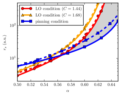
Figure 1: (Color online) Density-dependent bounds on the power functional for the the 3DEG. The dashed lines refer to the results from the variational ansatz and the solid lines correspond to numerical results. The blue (squares) lines separate the regions with pinned states (below the curves) and without pinned states (above the curves). The red (circles) and orange (triangles) lines denote boundary of the regions where the LO bound is obeyed (below the curves) and the regions where it is violated (above the curves) for different values of the constant $C$.

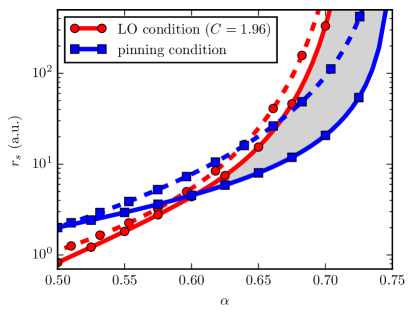
Figure 2: (Color online) Same as Fig. 1 but for the 2DEG. Here we only show the result for the tight LO-type bound in 2D ($C=1.96$) according to Ref. ourbound .

In Figs. 1 and 2 we show the results for the 3DEG and 2DEG, respectively. The solid lines correspond to critical densities obtained from numerical momentum distributions and the dashed lines refer to the variational ansatz for the momentum distributions discussed in Secs. II.1 (3DEG) and II.2 (2DEG). We plot the critical densities, characterized by the Wigner-Seitz radius $r_{s}$, as function of the exponent $\alpha=\beta/2$.

The two upper (red and orange) pairs of curves in Fig. 1 represent the critical densities for which the LO bound holds as an equality. The orange line corresponds to the original LO bound ($C=1.68$) and the red curve to the tighter LO bound ($C=1.44$) proposed in Ref. ourbound . In the region above the curves the LO bound is violated. Naturally, the tighter LO bound ($C=1.44$) leads to a smaller region of validity. The numerical results yield a slightly smaller region of validity than the ansatz. This means that $E_{xc}$ computed from the variational ansatz is larger and therefore violates the LO bound – which is a lower bound – for lower densities (or higher $r_{s}$). The fact that the LO curves for the ansatz and the numerical momentum distributions are very close to each other for the 3DEG indicates that the variational ansatz is very accurate – at least in the region close to the critical density determined by the LO bound.

The lower curves (blue) in Fig. 1 indicate the critical densities at which the momentum distribution acquires pinned states, i.e., above the curve we have $n({\bf k})<1$ for all ${\bf k}$ and below we have $n({\bf k})=1$ for some ${\bf k}$. Note that the ansatz for the momentum distribution breaks down below the dashed, blue curve. The numerical results for the momentum distribution below the solid, blue curve represent boundary minima of the RDMFT energy functional, which means that the Euler-Lagrange equation does not hold for wave vectors ${\bf k}$ with $n({\bf k})=1$. We see that the numerical momentum distributions increase the region of unpinned $n({\bf k})$. Since the ansatz becomes exact for $\alpha=0.5$ (or $\beta=1$) the solid and the dashed blue curves coincide at this value. However, the curves for the LO bound do not coincide at $\alpha=0.5$. Most likely this is due to the fact that the ansatz does not provide valid results below the pinning $r_{s}$. Hence, the $xc$ energies for the LO bound in the region below the dashed, blue curve are computed with momentum distributions that violate the Pauli constraint $0\leq n({\bf k})\leq 1$.

By comparing Figs. 1 and 2 we can see that the results from the variational ansatz are closer to the numerical results in the 3DEG than in the 2DEG. This indicates that the variational ansatz for the 3DEG is closer to the true momentum distribution than the variational ansatz for the 2DEG.

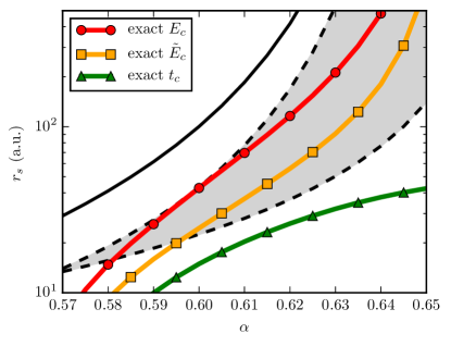
Figure 3: (Color online) Exact $E_{c}$ (red, circles), $\tilde{E}_{c}$ (orange, squares), and $t_{c}$ (green, triangles) for the 3DEG. Within the shaded region the tight LO bound ($C=1.44$) is satisfied and the momentum distribution is strictly smaller than one. The solid black line denotes the violation of the LO bound when the kinetic contribution to the correlations energy taken into account.

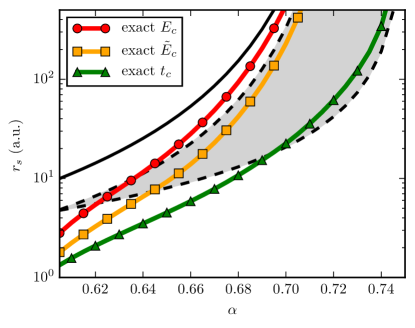
Figure 4: (Color online) Same as Fig. 3 but for the 2DEG. In the shaded region the tight LO bound ($C=1.96$) is satisfied and the momentum distribution is not pinned, i.e., $n(k)<1$. The solid black line denotes the violation of the LO bound when the kinetic contribution to the correlations energy taken into account.

Next we consider the correlation energies $E_{c}$ produced by the power functional. We remind that $E_{c}$ for the EG is known exactly from quantum Monte Carlo simulations for the 3DEG OB and the 2DEG AMGB . The total energy per particle of the EG is usually written as

$$\epsilon(r_{s})=\frac{A}{r_{s}^{2}}+\frac{B}{r_{s}}+e_{c}(r_{s})~{},$$ (27)

where $A$ and $B$ are well-known constants for the HF energy of the EG VignaleBook . The correlation energy, as implicitly defined in Eq. (27), contains a kinetic energy contribution $t_{c}$, or equivalently, we can decompose

$$\epsilon_{c}(r_{s})=t_{c}(r_{s})+\tilde{\epsilon}_{c}(r_{s})~{},$$ (28)

where $t_{c}$ is explicitly given by

$$t_{c}=\frac{1}{n}\frac{1}{(2\pi)^{d}}\int\!\!d{\bf k}k^{2}\Big{[}n(k)-n_{0}(k)\Big{]}~{}.$$ (29)

Here $n(k)$ is the momentum distribution of the interacting EG and $n_{0}(k)$ is the momentum distribution of the non-interacting EG, i.e., the Fermi step function. By using scaling relations, $\tilde{e}_{c}$ and $t_{c}$ can be obtained from the parameterizations of $e_{c}$ Takada .

In Figs. 3 and 4 we show the densities for which the total correlation energy $E_{c}$, the correlation energy without kinetic contribution $\tilde{E}_{c}$ and the kinetic correlation energy $t_{c}$ are exact as a function of $\alpha$. For the exact functional all three quantities would be exactly reproduced. However, we can see that for the power functional the three quantities are exact for different densities at the same power $\alpha$. This demonstrates the fact that even if the correlation energy is exact for a given density, the minimizing momentum distribution is not the exact momentum distribution.

We point out that for the 3DEG the kinetic contribution to the correlation energy is never exact in the region of the $\alpha$–$r_{s}$ plane for which $n(k)<1$ (cf. Fig. 3). For the 2DEG we find the somewhat surprising result that for $\alpha\gtrsim 0.64$ the correlation energy is exact for densities that violate the LO bound (cf. Fig. 4). This apparent contradiction can be resolved by remembering that $E_{c}$ contains kinetic contributions. Hence, we have plotted the solid black lines in both Figs. 3 and 4, which correspond to the critical densities for the violation of the LO bound when the kinetic correlation is included in $E_{xc}$ . Similarly we see that $\tilde{E}_{c}$, which excludes kinetic correlations, is always in the region of the $\alpha$–$r_{s}$ plane where the LO bound is obeyed.

IV Summary and conclusions

To summarize, we have numerically solved the minimizing momentum distributions for the power functional in both the three- and two-dimensional homogeneous electron gas. In particular, we have studied the ranges of validity for the power $\alpha$ and the density parameter $r_{s}$ in terms of satisfying the Lieb-Oxford lower bound for $E_{xc}$ and excluding the pinned states with $n({\bf k})=1$. The results have been compared to previous limits obtained from variational momentum distributions.

On the plane spanned by $\alpha$ and $r_{s}$, we have found regions of validity for the power functionals at $\alpha\gtrsim 0.57$ and $r_{s}\gtrsim 10$ in three dimensions and at $\alpha\gtrsim 0.60$ and $r_{s}\gtrsim 5$ in two dimensions. The lower boundaries of these regions in terms of $r_{s}$ – determined by the existence of pinned states – are pushed further to lower values when using the numerical solutions instead of the variational momentum distributions. However, the range of validity corresponds to relatively low densities, significantly lower than typical densities in, e.g., atoms, molecules, or clusters. In two dimensions, $r_{s}\sim 5$ could be realized in semiconductor quantum-dot systems reimann .

We have also computed the numerically exact correlation energies and their kinetic contributions (in terms of density-functional theory). The exact solutions partly coincide with the regimes of validity, but not with the same power $\alpha$ for both quantities $E_{c}$ and $t_{c}$. Therefore, the minimizing momentum distribution is not the exact one even if the correlation energy is exact for a given density.

- (1) P.-O. Löwdin, Phys. Rev. 97, 1474 (1955).
- (2) T. L. Gilbert, Phys. Rev. B 12, 2111 (1975).
- (3) For a review, see, e.g., R. M. Dreizler and E. K. U. Gross, Density Functional Theory (Springer, Berlin, 1990); U. von Barth, Phys. Scr. T109, 9 (2004).
- (4) D. R. Rohr, J. Toulouse, and K. Pernal, Phys. Rev. A 82, 052502 (2010).
- (5) K. J. H. Giesbertz, E. J. Baerends, and O. V. Gritsenko, Phys. Rev. Lett. 101, 033004 (2008).
- (6) N. N. Lathiotakis, N. Helbig, A. Rubio, and N. I. Gidopoulos, Phys. Rev. A 90, 032511 (2014).
- (7) T. Baldsiefen, A. Cangi, and E. K. U. Gross, Phys. Rev. A 92, 052514 (2015).
- (8) K. Pernal, J. Chem. Phys. 136, 184105 (2012).
- (9) S. Sharma, J. K. Dewhurst, S. Shallcross, and E. K. U. Gross, Phys. Rev. Lett. 110, 116403 (2013).
- (10) Y. Shinohara, S. Sharma, S. Shallcross, N. N. Lathiotakis, and E. K. U. Gross, J. Chem. Theor. Comp. 11, 4895 (2015).
- (11) S. Sharma, J. K. Dewhurst, N. N. Lathiotakis, and E. K. U. Gross, Phys. Rev. B 78, 201103(R) (2008).
- (12) N. N. Lathiotakis, N. Helbig, and E. K. U. Gross, Phys. Rev. B 75, 195120 (2007).
- (13) N. N. Lathiotakis, S. Sharma, J. K. Dewhurst, F. G. Eich, M. A. L. Marques, and E. K. U. Gross, Phys. Rev. A 79, 040501(R) (2009).
- (14) A. M. K. Müller, Phys. Lett. A 105, 446 (1984).
- (15) E. Tölö and A. Harju, Phys. Rev. B 81, 075321 (2010).
- (16) M. Levy, Density Matrices and Density Functionals, (Reidel, Dordrecht, 1987).
- (17) J. Cioslowski and K. Pernal, J. Chem. Phys. 111, 3396 (1999).
- (18) J. Cioslowski and K. Pernal, Phys. Rev. A 61, 034503 (2000).
- (19) A. Putaja and E. Räsänen, Phys. Rev. B 84, 035104 (2011).
- (20) E. H. Lieb, Phys. Lett. 70A, 444 (1979); E. H. Lieb and S. Oxford, Int. J. Quantum Chem. 19, 427 (1981).
- (21) E. Räsänen, S. Pittalis, K. Capelle, and C. R. Proetto, Phys. Rev. Lett. 102, 206406 (2009).
- (22) J. C. Kimball, J. Phys. A 8, 1513 (1975).
- (23) K. J. H. Giesbertz and R. van Leeuwen, J. Chem. Phys. 139, 104109 (2013).
- (24) M. Lewin and E. H. Lieb, Phys. Rev. A 91, 022507 (2015).
- (25) M. Seidl, S. Vuckovic, and P. Gori-Giorgi, Mol. Phys. (2016); doi:10.1080/00268976.2015.1136440.
- (26) E. H. Lieb, J. P. Solovej, and J. Yngvason, Phys. Rev. B 51, 10646 (1995).
- (27) T. Baldsiefen and E. K. U. Gross, Comput. Theor. Chem. 1003, 114 (2013).
- (28) G. F. Giuliani and G. Vignale, Quantum Theory of the Electron Liquid, (Cambridge University Press, 2005).
- (29) G. Ortiz, M. Harris, and P. Ballone, Phys. Rev. Lett. 82, 5317 (1999).
- (30) C. Attaccalite, S. Moroni, P. Gori-Giorgi, and G. B. Bachelet, Phys. Rev. Lett. 88, 256601 (2002).
- (31) Y. Takada and H. Yasuhara, Phys. Rev. B 44, 7879 (1991).
- (32) S. M. Reimann and M. Manninen, Rev. Mod. Phys. 74, 1283 (2002).