Radiative Seesaw-type Mechanism of Fermion Masses and Non-trivial Quark Mixing

Abstract

We propose a predictive inert two Higgs doublet model, where the standard Model (SM) symmetry is extended by $S_{3}\otimes Z_{2}\otimes Z_{12}$ and the field content is enlarged by extra scalar fields, charged exotic fermions and two heavy right-handed Majorana neutrinos. The charged exotic fermions generate a non-trivial quark mixing and provide one-loop-level masses for the first- and second-generation charged fermions. The masses of the light active neutrinos are generated from a one-loop-level radiative seesaw mechanism. Our model successfully explains the observed SM fermion mass and mixing pattern.

I Introduction

Despite its great success, the standard Model (SM) does not address several fundamental issues such as, for example, the number of fermion families and the observed pattern of fermion masses and mixing. As is known, in the quark sector the mixing is small while in the lepton sector two of the mixing angles are large. The three neutrino flavors mix with each other and at least two of the neutrinos have non-vanishing masses, which according to neutrino oscillation experimental data must be smaller than the SM charged fermion masses by many orders of magnitude. This so called “flavor puzzle” motivates extensions of the SM with larger scalar and/or fermion sector and with extended gauge groups, supplemented with discrete flavor symmetries, so that the resulting fermion mass matrix textures would explain the observed pattern of fermion masses and mixing. The implementation of these discrete flavor symmetries in several extensions of the SM is expected to provide an elegant solution of the “flavor puzzle” (for recent reviews on discrete flavor groups see, for instance, Refs. Ishimori:2010au ; Altarelli:2010gt ; King:2013eh ; King:2014nza ). In fact, considerable attention has already been paid in the literature to the $S_{3}$ Pakvasa:1977in ; Cardenas:2012bg ; Dias:2012bh ; Dev:2012ns ; Meloni:2012ci ; Canales:2013cga ; Ma:2013zca ; Kajiyama:2013sza ; Hernandez:2013hea ; Hernandez:2014lpa ; Hernandez:2014vta ; Vien:2014vka ; Ma:2014qra ; Das:2015sca ; Hernandez:2015dga ; Hernandez:2015zeh ; Hernandez:2016rbi ; Hernandez:2015hrt ; CarcamoHernandez:2016pdu ; Xing:2010iu $A_{4}$ Ma:2001dn ; Babu:2002dz ; Altarelli:2005yp ; Altarelli:2005yx ; deMedeirosVarzielas:2005qg ; He:2006dk ; Varzielas:2012ai ; Cooper:2012wf ; Ishimori:2012fg ; Ahn:2013mva ; Memenga:2013vc ; Bhattacharya:2013mpa ; Ferreira:2013oga ; Felipe:2013vwa ; Hernandez:2013dta ; King:2013hj ; Morisi:2013qna ; Morisi:2013eca ; Felipe:2013ie ; King:2014iia ; Karmakar:2014dva ; Campos:2014lla ; Hernandez:2015tna ; Karmakar:2015jza ; Pramanick:2015qga ; Bonilla:2016sgx ; Belyaev:2016oxy ; CarcamoHernandez:2017cwi ; CarcamoHernandez:2017kra , $S_{4}$ Yang:2011fh ; BhupalDev:2012nm ; Mohapatra:2012tb ; Varzielas:2012pa ; Ding:2013hpa ; Ishimori:2010fs ; Ding:2013eca ; Hagedorn:2011un ; Campos:2014zaa , $T_{7}$ Luhn:2007sy ; Hagedorn:2008bc ; Cao:2010mp ; Luhn:2012bc ; Kajiyama:2013lja ; Bonilla:2014xla ; Hernandez:2015cra ; Arbelaez:2015toa ; Hernandez:2015yxx and $\Delta(27)$ deMedeirosVarzielas:2006fc ; Ma:2006ip ; Varzielas:2012nn ; Bhattacharyya:2012pi ; Ferreira:2012ri ; Ma:2013xqa ; Nishi:2013jqa ; Varzielas:2013sla ; Aranda:2013gga ; Varzielas:2013eta ; Abbas:2014ewa ; Varzielas:2015aua ; Bjorkeroth:2015uou ; Chen:2015jta ; Abbas:2015zna ; Vien:2016tmh ; Hernandez:2016eod ; Chulia:2016giq ; CarcamoHernandez:2017owh flavor groups. Several models with discrete flavor symmetries, which bring about radiative seesaw mechanisms of fermion mass generation, have also been discussed in the literature Ma:1989ys ; Ma:1989cn ; Dong:2006gx ; Hernandez:2013mcf ; Adhikari:2015woo ; Nomura:2016emz ; Kownacki:2016hpm ; Nomura:2016ezz . A typical flaw of these models is the large number of free parameters and consequent limited predictive power, since they lack a mechanism underlying the observed hierarchy of quark mixing angles and masses. The experimental data suggest an empirical relation of the Cabbibo mixing angle to the first- and second-generation down-type quark masses $\sin\theta_{C}\sim\sqrt{\frac{m_{d}}{m_{s}}}$ Gatto:1968ss ; Cabibbo:1968vn ; Oakes:1969vm , which seems to imply a radiative seesaw mechanism of fermion mass generation, where the Cabbibo mixing arises from the down-type quark sector, whereas the up quark sector contributes to the remaining mixing angles. Inspired with this observation we propose an extension of the inert two Higgs doublet model (2HDM) realizing this idea. In our model a mismatch between the down- and up-type quark mass matrix textures is introduced, by distinguishing the two Higgs doublets with respect to the $Z_{2}$ flavor symmetry, preserved at all scales. One of these doublets–the SM Higgs–is $Z_{2}$-even, while another one is $Z_{2}$-odd. In order to maintain the $Z_{2}$-symmetry intact, we assume the latter to be VEV-less. The described setup is similar to the well-known inert 2HDM Deshpande:1977rw , but with the difference that here some of the SM fermions are $Z_{2}$-odd. Furthermore, compared to Ref. Deshpande:1977rw , the discrete symmetry in our model is extended from $Z_{2}$ to $S_{3}\otimes Z_{2}\otimes Z_{12}$, and the field content is enlarged by extra scalars, heavy charged exotic fermions and two heavy right-handed Majorana neutrinos. Note that only the $Z_{2}$ is preserved at low energies, whereas the $S_{3}\otimes Z_{12}$ symmetry is spontaneously broken. The latter allows us to explain the observed SM fermion mass and mixing pattern. In our modified inert 2HDM, the SM fermion mass and mixing pattern is due to a combination of tree and 1-loop-level effects. At tree level only the third generation charged fermions acquire masses and there is no quark mixing, while the first and second generation charged fermion masses and the quark mixing arise from one-loop-level radiative seesaw-type mechanism, triggered by virtual $Z_{2}$-charged scalar fields and electrically charged exotic fermions running inside the loops. Light active neutrino masses are generated from a one loop level radiative seesaw mechanism. Due to the preserved $Z_{2}$ symmetry, our model features natural dark matter candidates.

The following comparison of our model with the similar models in the literature could be in order. Despite the similar quality of the data description, our model is more predictive than the model of Ref. Branco:2010tx , since the latter, focused only on the quark sector, has a total of 12 free parameters, whereas the quark sector of our model is described by 9 free effective parameters, which are adjusted to reproduce the 10 physical observables of the quark sector. The models of Refs. Ishimori:2014jwa ; Ishimori:2014nxa ; Hernandez:2015zeh , Refs. CarcamoHernandez:2012xy ; Campos:2014zaa ; Hernandez:2015dga ; Hernandez:2013hea ; Hernandez:2014vta , Refs. Bhattacharyya:2012pi ; Vien:2014ica and Ref. Branco:2011wz possess in the quark sector 9, 10, 12, and 13 free parameters, respectively. For the lepton sector, our model is less predictive than in the quark sector, however, under some reasonable assumptions, the number of effective parameters in this sector can be reduced. As shown in detail in section III, our model can successfully accommodate the eight physical observables in the lepton sector, with only five effective free parameters for the case of normal neutrino mass hierarchy. With respect to the inverted neutrino mass hierarchy, more parameters are needed to successfully reproduce the masses and leptonic mixing angles.

The content of this paper goes as follows. In Sect. II we introduce the model setup. Section III deals with the derivation of fermion masses and mixings and provides our corresponding results. Our conclusions are stated in Sect. VI. Appendix A gives a brief description of the $S_{3}$ group. Appendix B shows the analytical expressions for the dimensionless parameters of the SM fermion mass matrices generated at one loop level.

II The Model

We consider a modified inert 2HDM, with the Standard Model gauge symmetry supplemented with the $S_{3}\otimes Z_{2}\otimes Z_{12}$ discrete group, and a scalar sector composed of 2 scalar SM doublets, i.e., $\phi_{1}$ and $\phi_{2}$ plus 4 scalar SM singlets. Out of these four SM scalar singlets, two scalar fields are grouped in a $S_{3}$ doublet, whereas the remaining ones are assigned to be one $S_{3}$ trivial singlet and one $S_{3}$ non-trivial singlet. The $Z_{2}$ symmetry is assumed to be preserved whereas the $S_{3}\otimes Z_{12}$ discrete group is broken at certain scale $\Lambda_{int}$. The fermion sector of the SM is extended to include four SM gauge singlet charged leptons $E_{1L}$, $E_{2L}$, $E_{1R}$ and $E_{2R}$, two right handed neutrinos $N_{1R}$, $N_{2R}$ and four $SU\left(2\right)_{L}$ singlet heavy quarks $T_{nL}$, $T_{nR}$, $B_{nL}$, $B_{nR}$ ($n=1,2$). The reasons for these specific choices will be explained below. It is assumed that the heavy exotic $T_{n}$ and $B_{n}$ quarks have electric charges equal to $\frac{2}{3}$ and $-\frac{1}{3}$, respectively. The $S_{3}\otimes Z_{2}\otimes Z_{12}$ assignments of the scalar fields are:

$$\phi_{1} \sim \left(\mathbf{1},1,1\right),\hskip 42.67912pt\phi_{2}\sim\left(\mathbf{1,}-1,1\right),$$

$$\xi \sim \left(\mathbf{2},1,1\right),\hskip 42.67912pt\eta\sim\left(\mathbf{1},-1,1\right),\hskip 42.67912pt\tau\sim\left(\mathbf{1}^{\prime},1,e^{-\frac{i\pi}{6}}\right).$$ (1)

The requirement of unbroken $Z_{2}$ symmetry implies that the $Z_{2}$ charged scalar fields $\phi_{2}$ and $\eta$ do not acquire vacuum expectation values. The remaining scalar fields, i.e., $\phi_{1}$, $\xi$ and $\tau$, which are neutral under the $Z_{2}$ symmetry, have non vanishing vacuum expectation values. Let us give a motivation for the above presented extension (1) of the scalar sector of the original inert 2HDM Deshpande:1977rw . One $Z_{2}$ odd SM singlet scalar $\eta$ (apart from the $Z_{2}$ odd scalar doublet $\phi_{2}$) is needed to implement the radiative seesaw mechanism of fermion mass generation. It yields a non-trivial quark mixing, provides masses for the first- and second-generation charged fermions and contributes to the light active neutrino masses. Furthermore, one $Z_{12}$-charged SM singlet scalar ($\tau$) is needed to generate the SM charged fermion mass and quark mixing pattern compatible with the observations. We also need an $S_{3}$-doublet scalar ($\xi$) to non-trivially couple it to the first- and second-generation right-handed SM down-type quarks, which we unify into an $S_{3}$-doublet.

We decompose the Higgs doublets $\phi_{1}$ and $\phi_{2}$ in the standard way as

$$\phi_{l} = \left(\begin{array}[]{c}\varphi_{l}^{+}\\ \frac{1}{\sqrt{2}}\left(v_{l}+\mathop{\mathrm{R}e}\phi_{l}^{0}+i\mathop{\mathrm{I}m}\phi_{l}^{0}\right)\end{array}\right),$$ (4)

$$v_{l} = v\delta_{l1},\hskip 19.91684ptl=1,2.$$ (5)

Here $v$ is a Higgs VEV breaking the electroweak symmetry.

The $S_{3}$-symmetry is broken by the VEV of the $S_{3}$ scalar doublet $\xi$. We choose the VEV alignment

$$\left\langle\xi\right\rangle=v_{\xi}\left(1,0\right),$$ (6)

compatible with the scalar potential minimization condition as demonstrated in Ref. Hernandez:2015dga . In the literature there have been constructed several $S_{3}$ flavor models with the similar VEV alignment of an $S_{3}$ scalar doublet (see for instance Refs. Hernandez:2013hea ; Hernandez:2014vta ; Hernandez:2015dga ; Hernandez:2015zeh ).

The $S_{3}\otimes Z_{2}\otimes Z_{12}$ assignments of the fermions of the model are as follows

$$q_{1L} \sim \left(\mathbf{1}^{\prime}\mathbf{,}1,1\right),\hskip 28.45274ptq_{2L}\sim\left(\mathbf{1},1,1\right),\hskip 28.45274ptq_{3L}\sim\left(\mathbf{1},1,1\right),\hskip 28.45274pt$$

$$u_{3R} \sim \left(\mathbf{1},1,1\right),\hskip 28.45274ptu_{1R}\sim\left(\mathbf{1}^{\prime},-1,-1\right),\hskip 28.45274ptu_{2R}\sim\left(\mathbf{1},-1,e^{\frac{i\pi}{3}}\right)$$

$$D_{R} = \left(d_{1R},d_{2R}\right)\sim\left(\mathbf{2},-1,e^{\frac{i\pi}{3}}\right),\hskip 28.45274ptd_{3R}\sim\left(\mathbf{1}^{\prime},1,i\right),$$

$$l_{1L} \sim \left(\mathbf{1},1,1\right),\hskip 28.45274ptl_{2L}\sim\left(\mathbf{1},1,1\right),\hskip 28.45274ptl_{3L}\sim\left(\mathbf{1},1,1\right),$$

$$l_{1R} \sim \left(\mathbf{1},-1,-1\right),\hskip 28.45274ptl_{2R}\sim\left(\mathbf{1}^{\prime},-1,i\right),\hskip 28.45274ptl_{3R}\sim\left(\mathbf{1}^{\prime},1,i\right),\hskip 28.45274pt$$

$$T_{1L} \sim \left(\mathbf{1},-1,1\right),\hskip 28.45274ptT_{1R}\sim\left(\mathbf{1}^{\prime},-1,1\right),\hskip 28.45274ptT_{2L}\sim\left(\mathbf{1},-1,1\right),\hskip 28.45274ptT_{2R}\sim\left(\mathbf{1},-1,1\right),$$

$$B_{1L} \sim \left(\mathbf{1},1,1\right),\hskip 28.45274ptB_{1R}\sim\left(\mathbf{1}^{\prime}\mathbf{,}-1,1\right),\hskip 28.45274ptB_{2L}\sim\left(\mathbf{1}^{\prime},1,1\right),\hskip 28.45274ptB_{2R}\sim\left(\mathbf{1,}-1,1\right),$$

$$E_{1L} \sim \left(\mathbf{1},-1,1\right),\hskip 28.45274ptE_{1R}\sim\left(\mathbf{1,-}1,1\right),\hskip 28.45274ptE_{2L}\sim\left(\mathbf{1},-1,1\right),\hskip 28.45274ptE_{2R}\sim\left(\mathbf{1,-}1,1\right),$$

$$N_{1R} \sim \left(\mathbf{1},-1,1\right),\hskip 28.45274ptN_{2R}\sim\left(\mathbf{1},-1,1\right).$$ (7)

Now it is timely to comment on the reasons for the introduction of the extended symmetry $S_{3}\otimes Z_{2}\otimes Z_{12}$. The $S_{3}$ symmetry reduces the number of parameters in the Yukawa sector of the model, improving its predictivity. The $Z_{12}$ symmetry shapes the hierarchical structure of the fermion mass matrices that gives rise to the observed charged fermion mass and quark mixing pattern. The preserved $Z_{2}$ symmetry selects the allowed entries in the quark mass matrices, so that the down-type quark sector contributes to the Cabbibo mixing, whereas the up-type quark sector contributes to the remaining mixing angles. The $Z_{2}$ symmetry allows also the implementation of a radiative seesaw type-mechanism (induced by the $Z_{2}$ charged scalar fields and the exotic charged fermions running in the internal lines of the loop), which gives rise to a non-trivial quark mixing and generates the masses for the first- and second-generation charged fermions. Besides that, due to the unbroken $Z_{2}$ symmetry, light active neutrino masses receive contributions from a one-loop radiative seesaw mechanism (induced by the $\eta$ and $\phi_{2}$ scalar fields and the heavy Majorana neutrinos $N_{1R}$ and $N_{2R}$ running in the internal lines of the loops). Let us note that the masses of the light active neutrinos are generated from a one-loop-level radiative seesaw mechanism. It is worth mentioning that in order to be compatible with the neutrino oscillation data, we need at least two light massive active neutrinos. Having only one right-handed Majorana neutrino, will lead to two massless active neutrinos, which is in clear contradiction with the experimental data on neutrino oscillation experiments. That is why we introduced in the model two massive right-handed neutrinos $N_{1R}$, $N_{2R}$, which is the minimal number necessary for this purpose, both for normal and inverted neutrino mass hierarchy. For similar reasons we introduced in our model four $SU\left(2\right)_{L}$ singlet heavy quarks $T_{nL}$, $T_{nR}$, $B_{nL}$, $B_{nR}$ ($n=1,2$), necessary to avoid the appearance of massless charged SM fermions.

With the above particle content, the following quark and lepton Yukawa terms, invariant under the symmetries of the model, arise:

$$\tciLaplace_{Y}^{q} = m_{T_{1}}\overline{T}_{1L}T_{1R}+m_{T_{2}}\overline{T}_{2L}T_{2R}+y_{3}^{\left(u\right)}\overline{q}_{3L}\widetilde{\phi}_{1}u_{3R}$$ (8)

$$+y_{1}^{\left(u\right)}\overline{q}_{1L}\widetilde{\phi}_{2}T_{1R}+x_{1}^{\left(u\right)}\overline{T}_{1L}\eta u_{3R}$$

$$+y_{2}^{\left(u\right)}\overline{q}_{2L}\widetilde{\phi}_{2}T_{2R}+x_{2}^{\left(u\right)}\overline{T}_{2L}\eta u_{3R}$$

$$+x_{3}^{\left(u\right)}\overline{T}_{1L}\eta u_{1R}\frac{\tau^{6}}{\Lambda^{6}}+x_{4}^{\left(u\right)}\overline{T}_{2L}\eta u_{2R}\frac{\tau^{2}}{\Lambda^{2}}$$

$$+m_{B_{1}}\overline{B}_{1L}B_{1R}+m_{B_{2}}\overline{B}_{2L}B_{2R}+y_{3}^{\left(d\right)}\overline{q}_{3L}\phi_{1}d_{3R}\frac{\tau^{3}}{\Lambda^{3}}$$

$$+x_{2}^{\left(d\right)}\overline{B}_{1L}\eta D_{R}\frac{\xi\tau^{2}}{\Lambda^{3}}+x_{4}^{\left(d\right)}\overline{B}_{2L}\eta D_{R}\frac{\xi\tau^{2}}{\Lambda^{3}}$$

$$+y_{1}^{\left(d\right)}\overline{q}_{1L}\phi_{2}B_{1R}+x_{1}^{\left(d\right)}\overline{B}_{1L}\eta D_{R}\frac{\xi\xi\tau^{2}}{\Lambda^{4}}$$

$$+y_{2}^{\left(d\right)}\overline{q}_{2L}\phi_{2}B_{2R}+x_{3}^{\left(d\right)}\overline{B}_{2L}\eta D_{R}\frac{\xi\xi\tau^{2}}{\Lambda^{4}}+h.c$$

$$\tciLaplace_{Y}^{l} = m_{E_{1}}\overline{E}_{1L}E_{1R}+m_{E_{2}}\overline{E}_{2L}E_{2R}+y_{3}^{\left(l\right)}\overline{l}_{3L}\phi_{1}l_{3R}\frac{\tau^{3}}{\Lambda^{3}}$$ (9)

$$+x_{1}^{\left(l\right)}\overline{l}_{1L}\phi_{2}E_{1R}+y_{1}^{\left(l\right)}\overline{E}_{1L}\eta l_{1R}\frac{\tau^{6}}{\Lambda^{6}}$$

$$+x_{2}^{\left(l\right)}\overline{l}_{2L}\phi_{2}E_{1R}+y_{2}^{\left(l\right)}\overline{E}_{1L}\eta l_{2R}\frac{\tau^{3}}{\Lambda^{3}}$$

$$+x_{3}^{\left(l\right)}\overline{l}_{1L}\phi_{2}E_{2R}+y_{3}^{\left(l\right)}\overline{E}_{2L}\eta l_{1R}\frac{\tau^{6}}{\Lambda^{6}}$$

$$+x_{4}^{\left(l\right)}\overline{l}_{2L}\phi_{2}E_{2R}+y_{4}^{\left(l\right)}\overline{E}_{2L}\eta l_{2R}\frac{\tau^{3}}{\Lambda^{3}}$$

$$+y_{11}^{\left(\nu\right)}\overline{l}_{1L}\widetilde{\phi}_{2}N_{1R}+y_{21}^{\left(\nu\right)}\overline{l}_{2L}\widetilde{\phi}_{2}N_{1R}$$

$$+y_{31}^{\left(\nu\right)}\overline{l}_{3L}\widetilde{\phi}_{2}N_{1R}+y_{12}^{\left(\nu\right)}\overline{l}_{1L}\widetilde{\phi}_{2}N_{2R}$$

$$+y_{22}^{\left(\nu\right)}\overline{l}_{2L}\widetilde{\phi}_{2}N_{2R}+y_{32}^{\left(\nu\right)}\overline{l}_{3L}\widetilde{\phi}_{2}N_{2R}$$

$$+m_{1N}\overline{N}_{1R}N_{1R}^{c}+m_{2N}\overline{N}_{2R}N_{2R}^{c}+h.c$$

Here we considered $S_{3}\otimes Z_{2}$ soft breaking mass terms for the charged exotic fermions. In addition, we have neglected the mixings between the $T_{1}$ ($B_{1}$) and $T_{2}$ ($B_{2}$) exotic quarks as well as the mixings between the $E_{1}$ and $E_{2}$ charged exotic leptons, by considering these charged exotic fermions as physical eigenstates. After the spontaneous breaking of the electroweak and $S_{3}\otimes Z_{12}$ discrete symmetries, these interactions generate at tree- and one-loop-levels the quark and lepton mass matrices. The one loop Feynman diagrams contributions to the fermion mass matrices are shown in Fig. 1.
The hierarchy of charged fermion masses and quark mixing angles arises in our model from the breaking of the $Z_{12}$ discrete group. In order to relate the quark masses with the quark mixing parameters, the VEVs of the SM scalar singlets $\xi$ and $\tau$ are set as follows:

$$v_{\xi}\sim\Lambda_{int}\sim v_{\tau}=\lambda\Lambda.$$ (10)

where $\lambda=0.225$ is one of the Wolfenstein parameters and $\Lambda$ corresponds to the model cutoff.

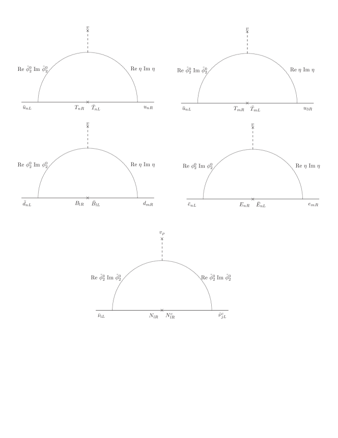
Figure 1: One loop Feynman diagrams contributions to the fermion mass matrices. Here $n=1,2$, $m=1,2$ and $l=1,2$.

From the quark Yukawa interactions it follows that the heavy exotic $T_{n}$ ($B_{n}$) quarks ($n=1,2$) will have a dominant decay mode into a SM up- (down-) type quark and a heavy CP even or CP odd neutral Higgs boson, which is identified as missing energy, due to the preserved $Z_{2}$ symmetry. Furthermore, from the lepton Yukawa interactions it follows that the charged exotic leptons $E_{n}$ ($n=1,2$) will decay dominantly into a SM charged lepton and a heavy CP even or CP odd neutral Higgs boson. The exotic $T_{n}$ and $B_{n}$ quarks are produced in pairs at the LHC via gluon fusion and the Drell-Yan mechanism, and the charged exotic leptons $E_{n}$ ($n=1,2$) are also produced in pairs but only via the Drell-Yan mechanism. Thus, observing an excess of events with respect to the SM background in the dijet and opposite sign dileptons final states can be a signal in support of this model at the LHC. On the other hand, it is worth mentioning that a heavy CP even Higgs can be produced at the LHC in association with a CP odd Higgs boson via Drell-Yan annihilation, with a cross section of about $0.1$ fb for heavy CP even and CP odd scalar masses of $600$ GeV and LHC center of mass energy of $\sqrt{s}=13$ TeV. To conclude this section, let us comment on the $h\rightarrow\gamma\gamma$ decay in our model, where $h$ is the $126$ GeV Higgs boson. In the standard model, this decay is dominated by $W$ loop diagrams, which can interfere destructively with the subdominant top quark loop; whereas In the 2HDM, the $h\rightarrow\gamma\gamma$ decay receives additional contributions from loops with charged scalars $H^{\pm}$, proportional to $\sin 2\beta$ (for the case where the Higgs doublets have different $Z_{N}$ charges), where $\tan\beta=v_{2}/v_{1}$ (cf. Ref. Hernandez:2015dga ). In our model $\tan\beta=0$ since $v_{2}=0$, and thus the charged Higgs boson contribution to the $126$ GeV Higgs diphoton decay is absent. From the explicit form of the $h\rightarrow\gamma\gamma$ decay rate given in Hernandez:2015dga for the 2HDM, it is easy to see that the Higgs diphoton decay rate in our model coincides with the SM expectation, since the light and heavy CP even neutral Higgs bosons do not mix, as a result of the preserved $Z_{2}$ symmetry.

III Quark masses and mixings

From the quark sector Yukawa terms (8) we find the quark mass matrices

$$M_{U} = \left(\begin{array}[]{ccc}\varepsilon_{11}^{\left(u\right)}\lambda^{6}&0&\varepsilon_{13}^{\left(u\right)}\\ 0&\varepsilon_{22}^{\left(u\right)}\lambda^{2}&\varepsilon_{23}^{\left(u\right)}\\ 0&0&y_{3}^{\left(u\right)}\end{array}\right)\frac{v}{\sqrt{2}},$$ (14)

$$M_{D} = \left(\begin{array}[]{ccc}\varepsilon_{11}^{\left(d\right)}\lambda^{4}&\varepsilon_{12}^{\left(d\right)}\lambda^{3}&0\\ \varepsilon_{21}^{\left(d\right)}\lambda^{4}&\varepsilon_{22}^{\left(d\right)}\lambda^{3}&0\\ 0&0&y_{3}^{\left(d\right)}\lambda^{3}\end{array}\right)\frac{v}{\sqrt{2}},$$ (18)

where $\varepsilon_{ij}^{\left(u,d\right)}$ are dimensionless parameters generated at one loop level whose corresponding expressions are given in Appendix B. In addition, $y_{3}^{\left(u\right)}$ and $y_{3}^{\left(d\right)}$ are $\mathcal{O}(1)$ dimensionless couplings generated at tree level from renormalizable and nonrenormalizable Yukawa terms, respectively.

Figure 2: Charm and strange quark masses randomly generated. The horizonal lines are the minimum and maximum values of the SM quark masses inside the $3\sigma$ experimentally allowed range.

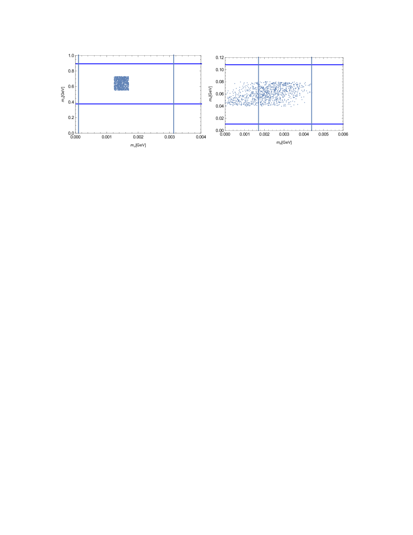
Figure 3: Correlations between the first and second generation SM quark masses. The horizonal and vertical lines are the minimum and maximum values of the second and first generation quark masses, respectively, inside the $3\sigma$ experimentally allowed range.

In order to show that the quark textures given above can fit the experimental data, and considering that the parameters $\varepsilon_{ij}^{\left(u,d\right)}$ are generated at one loop level, we choose a benchmark scenario where we set:

$$\varepsilon_{11}^{\left(u\right)} = a_{11}^{\left(u\right)}\lambda^{2},\hskip 28.45274pt\varepsilon_{22}^{\left(u\right)}=a_{22}^{\left(u\right)}\lambda^{2},\hskip 28.45274pt\varepsilon_{13}^{\left(u\right)}=a_{13}^{\left(u\right)}\lambda^{3},\hskip 28.45274pt\varepsilon_{23}^{\left(u\right)}=a_{23}^{\left(u\right)}\lambda^{2},$$

$$\varepsilon_{11}^{\left(d\right)} = a_{11}^{\left(d\right)}\lambda^{3},\hskip 28.45274pt\varepsilon_{21}^{\left(d\right)}=a_{21}^{\left(d\right)}\lambda^{2},\hskip 28.45274pt\varepsilon_{12}^{\left(d\right)}=a_{12}^{\left(d\right)}\lambda^{3},\hskip 28.45274pt\varepsilon_{22}^{\left(d\right)}=a_{22}^{\left(d\right)}\lambda^{2}.$$ (19)

where $a_{nn}^{\left(u\right)}$, $a_{n3}^{\left(u\right)}$, $a_{mn}^{\left(d\right)}$ ($m,n=1,2$) are $\mathcal{O}(1)$ parameters. Let us note that from the quark mass matrices given above, it follows that the Cabbibo mixing arises from the down-type quark sector, whereas the up-type quark sector contributes to the remaining mixing angles. Besides that, the low energy quark flavor data indicates that the CP violating phase in the quark sector is associated with the quark mixing angle in the 1-3 plane, as follows from the Standard parametrization of the quark mixing matrix. Consequently, in order to get quark mixing angles and a CP violating phase consistent with the experimental data, we assume that all dimensionless parameters given in Eqs. (14) and (18) are real, except $a_{13}^{\left(u\right)}$, which is taken to be complex. Since the observed pattern of charged fermion masses and quark mixing angles is generated from the $S_{3}\otimes Z_{12}$ symmetry breaking, and in order to have the right value of the Cabbibo mixing, we need $a_{21}^{\left(d\right)}\approx a_{22}^{\left(d\right)}$. In addition we set $y_{3}^{\left(u\right)}\approx 1$, as suggested by naturalness arguments. Then the quark sector of our model contains nine effective free parameters, i.e., $a_{11}^{\left(u\right)}$, $a_{22}^{\left(u\right)}$, $|a_{13}^{\left(u\right)}|$, $a_{23}^{\left(u\right)}$, $a_{11}^{\left(d\right)}$, $a_{12}^{\left(d\right)}$, $a_{22}^{\left(d\right)}$, $y_{3}^{\left(d\right)}$ and the phase $\arg\left(a^{\left(u\right)}_{13}\right)$, which are fitted to reproduce the ten physical observables of the quark sector, i.e., the six quark masses, the three mixing angles and the CP violating phase. By varying these parameters, we find the quark masses, the three quark mixing angles, and the CP violating phase $\delta$ reported in Table 1, which correspond to the best-fit values:

$$a_{23}^{\left(u\right)} \simeq 0.81,\hskip 28.45274pt|a_{13}^{\left(u\right)}|\simeq 0.3,\hskip 28.45274pt\arg\left(a^{\left(u\right)}_{13}\right)=-113^{\circ},\hskip 28.45274pta_{22}^{\left(u\right)}\simeq 1.43,\hskip 28.45274pta_{11}^{\left(u\right)}\simeq 1.27,$$

$$a_{11}^{\left(d\right)} \simeq 0.84,\hskip 28.45274pta_{12}^{\left(d\right)}\simeq 0.4,\hskip 28.45274pta_{22}^{\left(d\right)}\simeq 0.57,\hskip 28.45274pty_{3}^{\left(d\right)}\simeq 1.42.$$ (20)

Observable	Model value	Experimental value
$m_{u}(MeV)$	$1.47$	$1.45_{-0.45}^{+0.56}$
$m_{c}(MeV)$	$641$	$635\pm 86$
$m_{t}(GeV)$	$172.2$	$172.1\pm 0.6\pm 0.9$
$m_{d}(MeV)$	$3.00$	$2.9_{-0.4}^{+0.5}$
$m_{s}(MeV)$	$59.2$	$57.7_{-15.7}^{+16.8}$
$m_{b}(GeV)$	$2.82$	$2.82_{-0.04}^{+0.09}$
$\sin\theta_{12}$	$0.2257$	$0.2254$
$\sin\theta_{23}$	$0.0412$	$0.0413$
$\sin\theta_{13}$	$0.00352$	$0.00350$
$\delta$	$68^{\circ}$	$68^{\circ}$

Table 1: Model and experimental Olive:2016xmw ; Bora:2012tx ; Xing:2007fb values of the quark masses and CKM parameters.

It is worth mentioning, as follows from Eq. (69) given in Appendix B, that the functions $\varepsilon_{11}^{\left(u\right)}$, $\varepsilon_{22}^{\left(u\right)}$, $\varepsilon_{13}^{\left(u\right)}$ and $\varepsilon_{23}^{\left(u\right)}$ depend on the dimensionless parameters $x_{1}^{\left(u\right)}$, $x_{2}^{\left(u\right)}$, $x_{3}^{\left(u\right)}$, $x_{4}^{\left(u\right)}$, $y_{1}^{\left(u\right)}$, $y_{2}^{\left(u\right)}$, on the masses $m_{T_{1}}$, $m_{T_{2}}$, $m_{\mathop{\mathrm{R}e}\phi_{2}^{0}}$, $m_{\mathop{\mathrm{R}e}\eta}$, $m_{\mathop{\mathrm{I}m}\phi_{2}^{0}}$ and $m_{\mathop{\mathrm{I}m}\eta}$ as well as on the trilinear scalar coupling $C_{\phi_{2}\phi_{1}\eta}$.  Furthermore, the functions $\varepsilon_{11}^{\left(d\right)}$, $\varepsilon_{22}^{\left(d\right)}$, $\varepsilon_{12}^{\left(d\right)}$ and $\varepsilon_{21}^{\left(d\right)}$ depend on the dimensionless parameters $x_{1}^{\left(d\right)}$, $x_{2}^{\left(d\right)}$, $x_{3}^{\left(d\right)}$, $x_{4}^{\left(d\right)}$, $y_{1}^{\left(d\right)}$, $y_{2}^{\left(d\right)}$, on the masses $m_{B_{1}}$, $m_{B_{2}}$, $m_{\mathop{\mathrm{R}e}\phi_{2}^{0}}$, $m_{\mathop{\mathrm{R}e}\eta}$, $m_{\mathop{\mathrm{I}m}\phi_{2}^{0}}$ and $m_{\mathop{\mathrm{I}m}\eta}$ as well as on the trilinear scalar coupling $C_{\phi_{2}\phi_{1}\eta}$. Consequently, there is a good amount of parametric freedom to reproduce the obtained values for the $\varepsilon_{ij}^{\left(u,d\right)}$ ($i,j=1,2,3$) functions that successfully reproduce the physical observables of the quark sector. For instance, the best-fit values given above imply that $\varepsilon_{11}^{\left(u\right)}\simeq 6.4\times 10^{-2}$, which can be obtained by setting $m_{T_{1}}=1$ TeV, $m_{\mathop{\mathrm{R}e}\phi_{2}^{0}}=420$ GeV, $m_{\mathop{\mathrm{R}e}\eta}=560$ GeV, $m_{\mathop{\mathrm{I}m}\phi_{2}^{0}}=600$ GeV, $m_{\mathop{\mathrm{I}m}\eta}=800$ GeV, $C_{\phi_{2}\phi_{1}\eta}=3$ TeV, $x_{3}^{\left(u\right)}=y_{1}^{\left(u\right)}=3$. Similar considerations apply for the down-type quark and lepton sector.

In order to study the sensitivity of the obtained values for the SM quark masses under small variations around the best-fit values (maximum variation of $+0.2$, minimum of $-0.2$), we show in Fig. 2 the predicted charm and strange masses as functions of the iteration. We find that, for a slight deviation from the best-fit values, the obtained charm and strange masses stay inside the $3\sigma$ experimentally allowed range. We also have numerically checked that the remaining SM quark masses are kept inside the $3\sigma$ experimentally allowed limits when we perform small variations around the best-fit values, with the exception of the down and bottom quark masses. The sensitivity of the down-type quark mass under small variations around the best-fit values is due to the fact that all entries in the upper left block of the SM down-type quark mass matrix are different from zero, thus implying that there is an important region of parameter space where the determinant of the down-type quark mass matrix takes low values. With respect to the bottom quark mass, we find that most of the points are inside the $3\sigma$ experimentally allowed range. Those outside the $3\sigma$ experimentally allowed range correspond to values close to the lower and upper experimental bounds of the bottom quark mass. Consequently, our model is very predictive for the quark sector. Correlations between the first- and second-generation SM quark masses are shown in Fig. 3. The horizontal and vertical lines are the minimum and maximum values of the second- and first- generation quark masses, respectively, inside the $3\sigma$ experimentally allowed range.

IV Lepton masses and mixings

From the lepton Yukawa terms (9) we derive the neutrino mass matrices

$$M_{l} = \left(\begin{array}[]{ccc}\varepsilon_{11}^{\left(l\right)}\lambda^{6}&\varepsilon_{12}^{\left(l\right)}\lambda^{3}&0\\ \varepsilon_{21}^{\left(l\right)}\lambda^{6}&\varepsilon_{22}^{\left(l\right)}\lambda^{3}&0\\ 0&0&y_{3}^{\left(l\right)}\lambda^{3}\end{array}\right)\frac{v}{\sqrt{2}},$$ (24)

$$M_{\nu} = \left(\begin{array}[]{ccc}W_{1}^{2}&W_{1}W_{2}\cos\varphi&W_{1}W_{3}\cos\left(\varphi-\varrho\right)\\ W_{1}W_{2}\cos\varphi&W_{2}^{2}&W_{2}W_{3}\cos\varrho\\ W_{1}W_{3}\cos\left(\varphi-\varrho\right)&W_{2}W_{3}\cos\varrho&W_{3}^{2}\end{array}\right),$$ (28)

where $\varepsilon_{nm}^{\left(l\right)}$ ($n,m=1,2$) are dimensionless parameters generated at one loop level whose corresponding expressions are given in Appendix B. The parameters of the neutrino mass matrix of Eq. (28) take the form

$$\overrightarrow{W_{j}} = \left(\frac{A_{j1}\sqrt{m_{N_{1}}f_{1}^{\left(\nu\right)}}}{64\pi^{3}\Lambda},\frac{A_{j2}\sqrt{m_{N_{2}}f_{2}^{\left(\nu\right)}}}{64\pi^{3}\Lambda}\right),\hskip 14.22636ptj=1,2,3$$

$$\cos\varphi = \frac{\overrightarrow{W_{1}}\cdot\overrightarrow{W_{2}}}{\left|\overrightarrow{W_{1}}\right|\left|\overrightarrow{W_{2}}\right|},\hskip 7.11317pt\cos\left(\varphi-\varrho\right)=\frac{\overrightarrow{W}_{1}\cdot\overrightarrow{W_{3}}}{\left|\overrightarrow{W}_{1}\right|\left|\overrightarrow{W_{3}}\right|},\hskip 7.11317ptW_{j}=\left|\overrightarrow{W_{j}}\right|,$$

$$\cos\varrho = \frac{\overrightarrow{W_{2}}\cdot\overrightarrow{W_{3}}}{\left|\overrightarrow{W_{2}}\right|\left|\overrightarrow{W_{3}}\right|},\hskip 14.22636ptA_{js}=y_{js}^{\left(\nu\right)}\frac{v}{\sqrt{2}}\hskip 14.22636pts=1,2,$$

$$f_{s} = \frac{m_{R}^{2}}{m_{R}^{2}-m_{N_{s}}^{2}}\ln\left(\frac{m_{R}^{2}}{m_{N_{s}}^{2}}\right)-\frac{m_{I}^{2}}{m_{I}^{2}-m_{N_{s}}^{2}}\ln\left(\frac{m_{I}^{2}}{m_{N_{s}}^{2}}\right),$$

$$m_{R} = m_{\mathop{\mathrm{R}e}\phi_{2}^{0}},\hskip 28.45274ptm_{I}=m_{\mathop{\mathrm{I}m}\phi_{2}^{0}}.$$ (29)

In order to show that the lepton textures given above can fit the experimental data, and considering that the parameters $\varepsilon_{ij}^{\left(l\right)}$ are generated at one loop level, we choose a benchmark scenario where we set:

$$\varepsilon_{11}^{\left(l\right)}=a_{11}^{\left(l\right)}\lambda^{2},\hskip 28.45274pt\varepsilon_{21}^{\left(l\right)}=a_{21}^{\left(l\right)}\lambda^{2},\hskip 28.45274pt\varepsilon_{12}^{\left(l\right)}=a_{12}^{\left(l\right)}\lambda^{2},\hskip 28.45274pt\varepsilon_{22}^{\left(l\right)}=a_{22}^{\left(l\right)}\lambda^{2}.$$ (30)

where $a_{nm}^{\left(l\right)}$ ($n,m=1,2,3$) are $\mathcal{O}(1)$ parameters.

Then it follows that the charged lepton mass matrix takes the following form:

$$M_{l}=\frac{v}{\sqrt{2}}\left(\begin{array}[]{ccc}a_{11}^{\left(l\right)}\lambda^{8}&a_{12}^{\left(l\right)}\lambda^{5}&0\\ a_{21}^{\left(l\right)}\lambda^{8}&a_{22}^{\left(l\right)}\lambda^{5}&0\\ 0&0&y_{3}^{\left(l\right)}\lambda^{3}\end{array}\right).$$ (31)

which implies that the following relation is fulfilled:

$$M_{l}M_{l}^{T}=\frac{v^{2}}{2}\left(\begin{array}[]{ccc}\left(a_{12}^{\left(l\right)}\right)^{2}\lambda^{10}+\left(a_{11}^{\left(l\right)}\right)^{2}\lambda^{16}&a_{12}^{\left(l\right)}a_{22}^{\left(l\right)}\lambda^{10}+a_{11}^{\left(l\right)}a_{21}^{\left(l\right)}\lambda^{16}&0\\ a_{12}^{\left(l\right)}a_{22}^{\left(l\right)}\lambda^{10}+a_{11}^{\left(l\right)}a_{21}^{\left(l\right)}\lambda^{16}&\left(a_{22}^{\left(l\right)}\right)^{2}\lambda^{10}+\left(a_{21}^{\left(l\right)}\right)^{2}\lambda^{16}&0\\ 0&0&\left(y_{3}^{\left(l\right)}\right)^{2}\lambda^{6}\end{array}\right)\allowbreak.$$ (32)

The mass matrix $M_{l}M_{l}^{T}$ can be diagonalized by a rotation matrix $R_{l}$ according to

$$R_{l}^{T}M_{l}M_{l}^{T}R_{l}=\left(\begin{array}[]{ccc}m_{e}^{2}&0&0\\ 0&m_{\mu}^{2}&0\\ 0&0&m_{\tau}^{2}\end{array}\right),\hskip 28.45274pt\hskip 28.45274ptR_{l}=\left(\begin{array}[]{ccc}\cos\theta_{l}&\sin\theta_{l}&0\\ -\sin\theta_{l}&\cos\theta_{l}&0\\ 0&0&1\end{array}\right)\allowbreak,\hskip 28.45274pt\hskip 28.45274pt\tan\theta_{l}\simeq\frac{a_{12}^{\left(l\right)}}{a_{22}^{\left(l\right)}},$$ (33)

where the charged lepton masses are given by

$$m_{e} \simeq \lambda^{8}\cdot\frac{\left|a_{12}^{\left(l\right)}a_{21}^{\left(l\right)}-a_{11}^{\left(l\right)}a_{22}^{\left(l\right)}\right|}{\sqrt{\left(a_{12}^{\left(l\right)}\right)^{2}+\left(a_{22}^{\left(l\right)}\right)^{2}}}\frac{v}{\sqrt{2}},$$ (34)

$$m_{\mu} \simeq \lambda^{5}\cdot\sqrt{\left(a_{12}^{\left(l\right)}\right)^{2}+\left(a_{22}^{\left(l\right)}\right)^{2}}\frac{v}{\sqrt{2}},$$ (35)

$$m_{\tau} = \lambda^{3}\cdot y_{3}^{\left(l\right)}\frac{v}{\sqrt{2}}.$$ (36)

Thus we correctly reproduce the charged lepton mass hierarchy from the symmetry structure of the model.

To simplify further the analysis, we set $\varphi=\varrho$, obtaining that the light neutrino mass matrix is given by

$$M_{\nu}=\left(\begin{array}[]{ccc}W_{1}^{2}&\kappa W_{1}W_{2}&W_{1}W_{3}\\ \kappa W_{1}W_{2}&W_{2}^{2}&\kappa W_{2}W_{3}\\ W_{1}W_{3}&\kappa W_{2}W_{3}&W_{3}^{2}\end{array}\right),\hskip 56.9055pt\kappa=\cos\varphi.$$ (37)

Assuming that the neutrino Yukawa couplings are real, we find that for the normal (NH) and inverted (IH) mass hierarchies, the light neutrino mass matrix is diagonalized by a rotation matrix $R_{\nu}$, according to

$$R_{\nu}^{T}M_{\nu}R_{\nu} = \left(\begin{array}[]{ccc}0&0&0\\ 0&m_{\nu_{2}}&0\\ 0&0&m_{\nu_{3}}\end{array}\right)\allowbreak,\hskip 28.45274ptR_{\nu}=\left(\begin{array}[]{ccc}-\frac{W_{3}}{\sqrt{W_{1}^{2}+W_{3}^{2}}}&\frac{W_{1}}{\sqrt{W_{1}^{2}+W_{3}^{2}}}\sin\theta_{\nu}&\frac{W_{1}}{\sqrt{W_{1}^{2}+W_{3}^{2}}}\cos\theta_{\nu}\\ 0&\cos\theta_{\nu}&-\sin\theta_{\nu}\\ \frac{W_{1}}{\sqrt{W_{1}^{2}+W_{3}^{2}}}&\frac{W_{3}}{\sqrt{W_{1}^{2}+W_{3}^{2}}}\sin\theta_{\nu}&\frac{W_{3}}{\sqrt{W_{1}^{2}+W_{3}^{2}}}\cos\theta_{\nu}\end{array}\right),\hskip 14.22636pt\mbox{for NH}$$ (44)

$$\tan\theta_{\nu} = -\sqrt{\frac{W_{2}^{2}-m_{\nu_{2}}}{m_{\nu_{3}}-W_{2}^{2}}}$$ (45)

$$m_{\nu_{1}} = 0,\hskip 14.22636ptm_{\nu_{2,3}}=\frac{W_{1}^{2}+W_{2}^{2}+W_{3}^{2}}{2}\mp\frac{\sqrt{\left(W_{1}^{2}-W_{2}^{2}+W_{3}^{2}\right)^{2}+4\kappa^{2}W_{2}^{2}\left(W_{1}^{2}+W_{3}^{2}\right)}}{2}.$$ (46)

$$R_{\nu}^{T}M_{\nu}R_{\nu} = \left(\begin{array}[]{ccc}m_{\nu_{1}}&0&0\\ 0&m_{\nu_{2}}&0\\ 0&0&0\end{array}\right)\allowbreak,\hskip 28.45274ptR_{\nu}=\left(\begin{array}[]{ccc}\frac{W_{1}}{\sqrt{W_{1}^{2}+W_{3}^{2}}}\sin\theta_{\nu}&\frac{W_{1}}{\sqrt{W_{1}^{2}+W_{3}^{2}}}\cos\theta_{\nu}&-\frac{W_{3}}{\sqrt{W_{1}^{2}+W_{3}^{2}}}\\ \cos\theta_{\nu}&-\sin\theta_{\nu}&0\\ \frac{W_{3}}{\sqrt{W_{1}^{2}+W_{3}^{2}}}\sin\theta_{\nu}&\frac{W_{3}}{\sqrt{W_{1}^{2}+W_{3}^{2}}}\cos\theta_{\nu}&\frac{W_{1}}{\sqrt{W_{1}^{2}+W_{3}^{2}}}\end{array}\right),\hskip 14.22636pt\mbox{for IH}$$ (53)

$$\tan\theta_{\nu} = -\sqrt{\frac{W_{2}^{2}-m_{\nu_{1}}}{m_{\nu_{2}}-W_{2}^{2}}}$$ (54)

$$m_{\nu_{1,2}} = \frac{W_{1}^{2}+W_{2}^{2}+W_{3}^{2}}{2}\mp\frac{1}{2}\sqrt{\left(W_{1}^{2}-W_{2}^{2}+W_{3}^{2}\right)^{2}+4\kappa^{2}W_{2}^{2}\left(W_{1}^{2}+W_{3}^{2}\right)},\hskip 14.22636ptm_{\nu_{3}}=0.$$ (55)

With the rotation matrices in the charged lepton sector $R_{l}$, given by Eq. (33), and in the neutrino sector $R_{\nu}$, given by Eqs. (44) and (53) for NH and IH, respectively, we find the PMNS mixing matrix:

$$U=R_{l}^{T}R_{\nu}=\left\{\begin{array}[]{l}\left(\begin{array}[]{ccc}-\frac{W_{3}}{\sqrt{W_{1}^{2}+W_{3}^{2}}}\cos\theta_{l}&\frac{W_{1}}{\sqrt{W_{1}^{2}+W_{3}^{2}}}\cos\theta_{l}\sin\theta_{\nu}-\cos\theta_{\nu}\sin\theta_{l}&\sin\theta_{l}\sin\theta_{\nu}+\frac{W_{1}}{\sqrt{W_{1}^{2}+W_{3}^{2}}}\cos\theta_{l}\cos\theta_{\nu}\\ -\frac{W_{3}}{\sqrt{W_{1}^{2}+W_{3}^{2}}}\sin\theta_{l}&\cos\theta_{l}\cos\theta_{\nu}+\frac{W_{1}}{\sqrt{W_{1}^{2}+W_{3}^{2}}}\sin\theta_{\nu}\sin\theta_{l}&\frac{W_{1}}{\sqrt{W_{1}^{2}+W_{3}^{2}}}\sin\theta_{l}\cos\theta_{\nu}-\cos\theta_{l}\sin\theta_{\nu}\\ \frac{W_{1}}{\sqrt{W_{1}^{2}+W_{3}^{2}}}&\frac{W_{3}}{\sqrt{W_{1}^{2}+W_{3}^{2}}}\sin\theta_{\nu}&\frac{W_{3}}{\sqrt{W_{1}^{2}+W_{3}^{2}}}\cos\theta_{\nu}\end{array}\right)\ \ \ \ \ \mbox{for NH},\\ \left(\begin{array}[]{ccc}\frac{W_{1}}{\sqrt{W_{1}^{2}+W_{3}^{2}}}\cos\theta_{l}\sin\theta_{\nu}-\cos\theta_{\nu}\sin\theta_{l}&\sin\theta_{l}\sin\theta_{\nu}+\frac{W_{1}}{\sqrt{W_{1}^{2}+W_{3}^{2}}}\cos\theta_{l}\cos\theta_{\nu}&-\frac{W_{3}}{\sqrt{W_{1}^{2}+W_{3}^{2}}}\cos\theta_{l}\\ \cos\theta_{l}\cos\theta_{\nu}+\frac{W_{1}}{\sqrt{W_{1}^{2}+W_{3}^{2}}}\sin\theta_{l}\sin\theta_{\nu}&\frac{W_{1}}{\sqrt{W_{1}^{2}+W_{3}^{2}}}\cos\theta_{\nu}\sin\theta_{l}-\cos\theta_{l}\sin\theta_{\nu}&-\frac{W_{3}}{\sqrt{W_{1}^{2}+W_{3}^{2}}}\sin\theta_{l}\\ \frac{W_{3}}{\sqrt{W_{1}^{2}+W_{3}^{2}}}\sin\theta_{\nu}&\frac{W_{3}}{\sqrt{W_{1}^{2}+W_{3}^{2}}}\cos\theta_{\nu}&\frac{W_{1}}{\sqrt{W_{1}^{2}+W_{3}^{2}}}\end{array}\right)\allowbreak\ \ \ \ \mbox{for IH}.\end{array}\right.$$ (56)

From the standard parametrization of the leptonic mixing matrix, it follows that the lepton mixing angles for NH and IH, respectively, are

$$\sin^{2}\theta_{12} = \frac{\left(\frac{W_{1}}{\sqrt{W_{1}^{2}+W_{3}^{2}}}\cos\theta_{l}\sin\theta_{\nu}-\cos\theta_{\nu}\sin\theta_{l}\right)^{2}}{1-\left(\sin\theta_{l}\sin\theta_{\nu}+\frac{W_{1}}{\sqrt{W_{1}^{2}+W_{3}^{2}}}\cos\theta_{l}\cos\theta_{\nu}\right)^{2}},\hskip 28.45274pt\sin^{2}\theta_{13}=\left(\sin\theta_{l}\sin\theta_{\nu}+\frac{W_{1}}{\sqrt{W_{1}^{2}+W_{3}^{2}}}\cos\theta_{l}\cos\theta_{\nu}\right)^{2},$$

$$\sin^{2}\theta_{23} = \frac{\left(\frac{W_{1}}{\sqrt{W_{1}^{2}+W_{3}^{2}}}\sin\theta_{l}\cos\theta_{\nu}-\cos\theta_{l}\sin\theta_{\nu}\right)^{2}}{1-\left(\sin\theta_{l}\sin\theta_{\nu}+\frac{W_{1}}{\sqrt{W_{1}^{2}+W_{3}^{2}}}\cos\theta_{l}\cos\theta_{\nu}\right)^{2}}\ ,\ \ \ \ \ \ \ \ \mbox{for NH}$$ (57)

$$\sin^{2}\theta_{12} = \frac{\left(\sin\theta_{l}\sin\theta_{\nu}+\frac{W_{1}}{\sqrt{W_{1}^{2}+W_{3}^{2}}}\cos\theta_{l}\cos\theta_{\nu}\right)^{2}}{1-\frac{W_{3}^{2}\cos^{2}\theta_{l}}{W_{1}^{2}+W_{3}^{2}}},\hskip 48.36967pt\sin^{2}\theta_{13}=\frac{W_{3}^{2}\cos^{2}\theta_{l}}{W_{1}^{2}+W_{3}^{2}},$$

$$\sin^{2}\theta_{23} = \frac{\frac{W_{3}^{2}}{W_{1}^{2}+W_{3}^{2}}\sin^{2}\theta_{l}}{1-\frac{W_{3}^{2}\cos^{2}\theta_{l}}{W_{1}^{2}+W_{3}^{2}}}\ ,\hskip 159.33542pt\mbox{for IH}$$ (58)

In the charged lepton sector the model has five free parameters $a_{11}^{(l)},a_{12}^{(l)},a_{21}^{(l)},a_{22}^{(l)},y_{3}^{(l)}$. Fitting Eqs. (34)-(36) for $m_{e,\mu,\tau}$ to the corresponding experimental values Bora:2012tx , we found $\mathcal{O}(1)$ solutions for these parameters. Therefore, we conclude that the model correctly predicts the charged lepton mass hierarchy according to Eqs. (34)-(36). On the other hand, it does not predict the particular values of the charged lepton masses. In fact, within the hierarchical structure incorporated in Eqs. (34)-(36), the five free $\mathcal{O}(1)$ parameters $a_{11}^{(l)},a_{12}^{(l)},a_{21}^{(l)},a_{22}^{(l)},y_{3}^{(l)}$ allow to reproduce the experimental values of $m_{e,\mu,\tau}$ with arbitrary precision limited only by the experimental errors.

The charged lepton sector “contributes” to the neutrino sector with a single free parameter $\theta_{l}$ defined in Eq. (33). It remains unrestricted by the charged lepton masses. Thus, in the neutrino sector we have five free parameters $W_{1,2,3},\kappa,\theta_{l}$ and five observables: two neutrino mass squared splittings $\Delta m_{21}^{2}$, $\Delta m_{31}^{2}$ (we define $\Delta m_{ij}^{2}=m_{i}^{2}-m_{j}^{2}$) and three mixing angles $\sin^{2}\theta_{12}$, $\sin^{2}\theta_{13}$, $\sin^{2}\theta_{23}$ for both NH and IH. We solve Eqs. (46), (55) and (57), (58) with respect to the model parameters for the central values of the corresponding observables shown in Table 2. The unique solutions for NH and IH are

for NH: $$\kappa\simeq 0.7,\hskip 42.67912ptW_{1}\simeq 0.09\,\mbox{eV}^{\frac{1}{2}},\ \ W_{2}\simeq 0.16\mbox{eV}^{\frac{1}{2}},\ \ W_{3}\simeq 0.15\,\mbox{eV}^{\frac{1}{2}},\ \ \theta_{l}\simeq 18.95^{\circ}$$ (59)

forIH: $$\kappa\simeq 6.11\times 10^{-3},\ \ W_{1}\simeq 0.14\,\mbox{eV}^{\frac{1}{2}},\ \ W_{2}\simeq 0.22\,\mbox{eV}^{\frac{1}{2}},\ \ W_{3}\simeq 0.17\,\mbox{eV}^{\frac{1}{2}},\ \ \theta_{l}\simeq-78.30^{\circ}.$$ (60)

Fig. 4 shows the correlation between $\Delta m_{21}^{2}$ and $\Delta m_{31}^{2}$ for the cases of normal and inverted neutrino mass hierarchies, respectively. We find that a slight variation from the best-fit values yields, for several points of the parameter space, an important deviation in the values of the neutrino mass squared splittings and leptonic mixing parameters, especially for the case of inverted neutrino mass hierarchy.

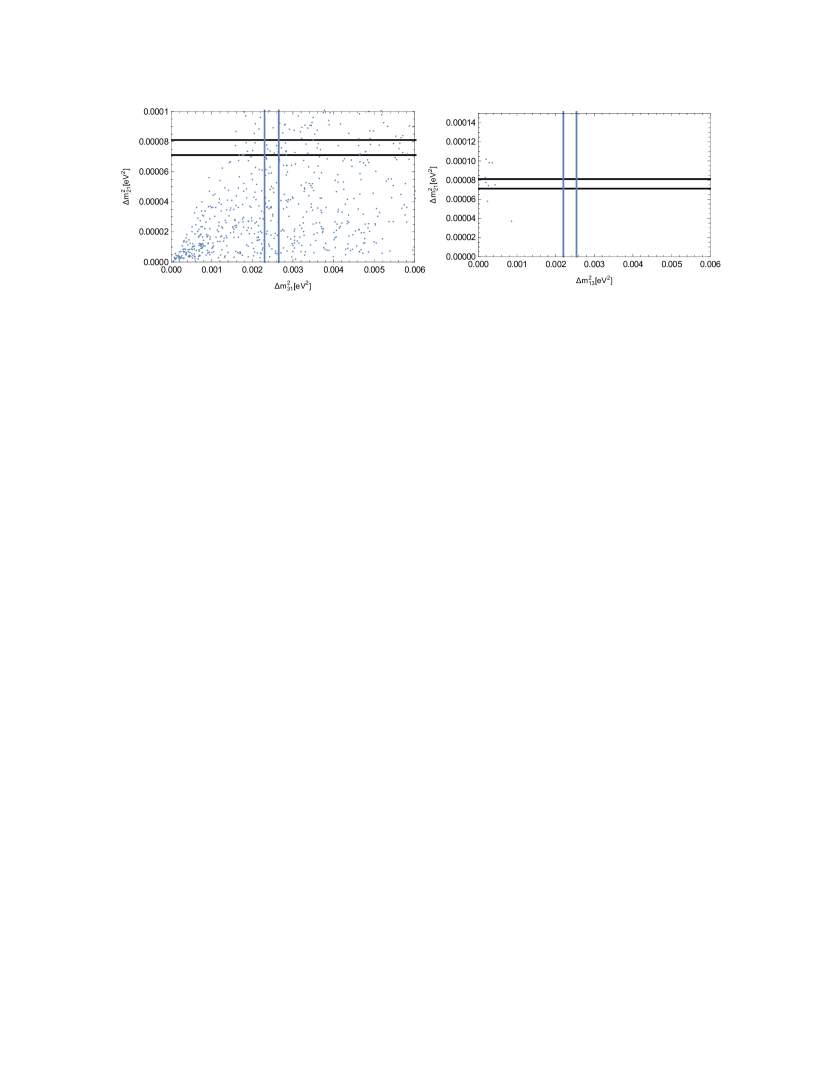
Figure 4: Correlations between $\Delta m_{21}^{2}$ and $\Delta m_{31}^{2}$ for the cases of normal (left plot) and inverted (right plot) neutrino mass hierarchy. The horizonal and vertical lines are the minimum and maximum values of the neutrino mass squared splittings inside the $3\sigma$ experimentally allowed range.

Observable	Experimental value	(i)	(ii)’	(ii)
$m_{e}(MeV)$	$0.487$	no prediction	input	0.43
$m_{\mu}(MeV)$	$102.8\pm 0.0003$	no prediction	113.07	115.1
$\Delta m_{21}^{2}$($10^{-5}$eV2) (NH)	$7.60_{-0.18}^{+0.19}$	7.62	7.72	7.62
$\Delta m_{31}^{2}$($10^{-3}$eV2) (NH)	$2.48_{-0.07}^{+0.05}$	2.52	2.70	2.52
$\sin^{2}\theta_{12}$ (NH)	$0.323\pm 0.016$	0.324	0.258	0.303
$\sin^{2}\theta_{23}$ (NH)	$0.567_{-0.128}^{+0.032}$	0.542	0.526	0.527
$\sin^{2}\theta_{13}$ (NH)	$0.0234\pm 0.0020$	0.0234	0.0224	0.0204
$\Delta m_{21}^{2}$($10^{-5}$eV2) (IH)	$7.60_{-0.18}^{+0.19}$	-	-	-
$\Delta m_{13}^{2}$($10^{-3}$eV2) (IH)	$2.38_{-0.06}^{+0.05}$	-	-	-
$\sin^{2}\theta_{12}$ (IH)	$0.323\pm 0.016$	-	-	-
$\sin^{2}\theta_{23}$ (IH)	$0.573_{-0.043}^{+0.025}$	-	-	-
$\sin^{2}\theta_{13}$ (IH)	$0.0240\pm 0.0019$	-	-	-

Table 2: The symmetry inspired benchmark scenarios (i) and (ii) versus the experimental values of the charged lepton masses Bora:2012tx , neutrino oscillation observables for the normal (NH) and inverted (IH) mass hierarchies Forero:2014bxa . Scenario (i): the four model parameters (62) fit the five neutrino oscillation observables for the NH. Scenario (ii)’: from the experimental input value $m_{e}=0.487$MeV we determine a model parameter $a_{12}^{(l)}=0.52$ and then calculate $m_{\mu}=113.07$MeV; the neutrino oscillation observables for the NH are fitted with three parameters (63). Scenario (ii)’: the same as (ii), but fitting jointly the four model parameters (64) to the seven observables.

Nevertheless the model in its present version is not predictive in the lepton sector except for the charged lepton mass hierarchy Eqs. (34)-(36). This is because the number of free parameters equals the number of observables.

However, considering the model parameters for NH in Eq.  (59) we note that their numerical values $W_{2}\simeq W_{3}$, $\kappa\approx 1$ may point to an approximate underlying $\mu-\tau$ symmetry. In fact for $W_{2}=W_{3}$, $\kappa=1$ the light active neutrino mass matrix (37) coincides in structure with the $\mu-\tau$ symmetric Fukuyama-Nishiura texture Fukuyama:1997ky :

$$M_{\nu}=\left(\begin{array}[]{ccc}A&B&B\\ B&C&D\\ B&D&C\end{array}\right).$$ (61)

With this observation let us study a $\mu-\tau$-symmetry inspired benchmark scenario in our model. Incorporation of the $\mu-\tau$-symmetry in our model implies $W_{2}=W_{3}$ and $\kappa=1$ and, therefore, $C=D$ in (61) leading to two vanishing eigenvalues, which is in clear contradiction with the neutrino oscillation data. After all this symmetry cannot be exact, since it is explicitly broken in the charged lepton sector (for more details on the phenomenological aspects of the $\mu-\tau$ interchange symmetry see, for instance, Refs.  Mohapatra:2004mf ). However, the $\mu-\tau$-symmetry can be incorporated in our model as a “minimally” broken symmetry. Its maximal breaking corresponds to the violation of both $W_{2}=W_{3}$ and $\kappa=1$ conditions. In this sense the minimal breaking is introduced by the violation of only one of these conditions. As can easily be checked the case $W_{2}\neq W_{3}$ with $\kappa=1$ is an inappropriate one since it has two zero eigenvalues of the neutrino mass matrix Eq. (37). Thus, we study the benchmark scenario
(i) with $W_{2}=W_{3}$ and $\kappa$ being a free $\mu-\tau$-symmetry breaking parameter. In this case there is only one zero neutrino mass matrix eigenvalue. Now we have four free model parameters $W_{1}$, $W_{2}$, $\kappa$ and $\theta_{l}$ versus the five physical observables in the neutrino sector, i.e., the two neutrino mass squared splittings and the three leptonic mixing parameters. Thus, the model is able to predict one of these observables using the experimental values of the other four. Instead of doing this we conventionally fit the model parameters to the experimental values of all the five observables within the corresponding experimental errors. The best fit results are shown in Table 2 for

$$\kappa \simeq 0.70,\hskip 28.45274ptW_{1}\simeq 0.09\mbox{eV}^{\frac{1}{2}},\hskip 28.45274ptW_{2}\simeq 0.16\mbox{eV}^{\frac{1}{2}},\hskip 28.45274pt\theta_{l}\simeq 19.81^{\circ}.$$ (62)

corresponding to the normal neutrino hierarchy. Here the parameter $\kappa$ is not too far from its $\mu-\tau$-symmetric value $\kappa=1$. In the case of the inverted hierarchy it is two-three orders of magnitude away from from this value and the $\mu-\tau$-symmetry does not show up as an approximate symmetry of the neutrino sector. A more detailed study of this observation and its possible implementation in the model Lagrangian will be addressed elsewhere.

Let us examine even more restrictive benchmark scenario assuming additionally to $W_{3}=W_{2}$ also the relation for the model parameters $a_{11}^{\left(l\right)}=a_{22}^{\left(l\right)}=a_{21}^{\left(l\right)}=1$ in the sector of charged leptons $e,\mu$. So that there is only one free parameter $a_{12}^{\left(l\right)}$ to fit $m_{e}$ and $m_{\mu}$ using Eqs. (34)-(35). This scenario is motivated by the fact we already discussed above (see the paragraph after Eqs. (58)) that our model correctly reproduces the charged lepton mass hierarchy with all the parameters $a_{11}^{(l)},a_{12}^{(l)},a_{21}^{(l)},a_{22}^{(l)}$ of the order $\mathcal{O}(1)$. Setting all these parameters to be $a_{ij}^{(l)}=1$ leads to a rather rough estimate of $m_{e}$ and $m_{\mu}$. Moreover, in this case $\tan\theta_{l}=1$, which is incompatible with the neutrino oscillation data as seen from (62). Therefore, we release $a_{12}^{(l)}$ assuming it to be the only free parameter in the $e-\mu$-sector of charged leptons. Thus we consider a benchmark scenario
(ii) with $a_{11}^{\left(l\right)}=a_{22}^{\left(l\right)}=a_{21}^{\left(l\right)}=1$, $W_{2}=W_{3}$. There are only four free parameters are $W_{1},W_{2},\kappa$ and $a_{12}^{(l)}$ to reproduce seven observable: $m_{e},m_{\mu}$ and five neutrino oscillation parameters. Note that the charged lepton $e-\mu$-sector depends only on one of these parameters, namely, $a_{12}^{(l)}$. It is tempting to try to make a prediction for $m_{\mu}$ starting from the best measured $m_{e}$. This also restricts the number of the free parameters in the neutrino sector down to $W_{1},W_{2},\kappa$. In this way we solve Eq. (34) with respect to $a_{12}^{(l)}$ for the central experimental value of $m_{e}$ and predict $m_{\mu}$ using (35). The result is shown in Table 2 in the column (ii)’ for $a_{12}^{(l)}=0.52$ obtained from $m_{e}$. In the neutrino sector, having three parameters, the model is able to predict any two of the five observables using as an input the experimental values of the other three. However, as in the scenario (i) we fit all the neutrino oscillation observables, $\Delta m_{21}^{2}$, $\Delta m_{31}^{2}$, $\sin^{2}\theta_{12}$, $\sin^{2}\theta_{13}$, $\sin^{2}\theta_{23}$ with the model parameters $W_{1},W_{2},\kappa$. The best fit values shown in the column (ii)’ of Table 2 correspond to

$$\kappa=0.71,\ \ \ W_{1}=0.05\mbox{eV}^{\frac{1}{2}},\ \ \ W_{2}=-0.17\mbox{eV}^{\frac{1}{2}}.$$ (63)

Now, instead of fixing $a_{12}^{(l)}$ from $m_{e}$, we fit all the model parameters $W_{1},W_{2},\kappa,a_{12}^{(l)}$ to seven observables $m_{e},m_{\mu}$ and $\Delta m_{21}^{2}$, $\Delta m_{31}^{2}$, $\sin^{2}\theta_{12}$, $\sin^{2}\theta_{13}$, $\sin^{2}\theta_{23}$. The best-fit values are shown in the column (ii) of Table 2 and correspond to the following values of the model parameters:

$$\kappa \simeq 0.71,\hskip 28.45274ptW_{1}\simeq 0.06\mbox{eV}^{\frac{1}{2}},\hskip 28.45274ptW_{2}\simeq-0.17\mbox{eV}^{\frac{1}{2}},\hskip 28.45274pta_{12}^{\left(l\right)}\simeq 0.56.$$ (64)

As seen from Table 3 in the scenario (ii) the neutrino oscillation parameters $\sin^{2}\theta_{12}$, $\sin^{2}\theta_{23}$, $\Delta m_{21}^{2}$, $\Delta m_{31}^{2}$ are inside the $1\sigma$ experimentally allowed range. The reactor mixing parameter $\sin^{2}\theta_{13}$ is inside the $2\sigma$ range.

Now we evaluate in our model the effective Majorana neutrino mass parameter of neutrinoless double beta ($0\nu\beta\beta$) decay

$$m_{\beta\beta}=\left|\sum_{j}U_{ek}^{2}m_{\nu_{k}}\right|,$$ (65)

where $U_{ej}^{2}$ and $m_{\nu_{k}}$ are the PMNS mixing matrix elements and the Majorana neutrino masses, respectively.

Parameter	$\Delta m_{21}^{2}$($10^{-5}$eV2)	$\Delta m_{31}^{2}$($10^{-3}$eV2)	$\left(\sin^{2}\theta_{12}\right)_{\exp}$	$\left(\sin^{2}\theta_{23}\right)_{\exp}$	$\left(\sin^{2}\theta_{13}\right)_{\exp}$
Best fit	$7.60$	$2.48$	$0.323$	$0.567$	$0.0234$
$1\sigma$ range	$7.42-7.79$	$2.41-2.53$	$0.307-0.339$	$0.439-0.599$	$0.0214-0.0254$
$2\sigma$ range	$7.26-7.99$	$2.35-2.59$	$0.292-0.357$	$0.413-0.623$	$0.0195-0.0274$
$3\sigma$ range	$7.11-8.11$	$2.30-2.65$	$0.278-0.375$	$0.392-0.643$	$0.0183-0.0297$

Table 3: Range for experimental values of neutrino mass squared splittings and leptonic mixing parameters, taken from Ref. Forero:2014bxa , for the case of normal hierarchy.

As we already mentioned the model parameters in Eq. (28) may have arbitrary complex phases. Therefore there may occur cancellation between the terms in Eq. (65), which we are not able to control in the model. Thus we can predict only upper bounds for $m_{\beta\beta}$. For the parameters (59), (60) we find

$$m_{\beta\beta}\leq\left\{\begin{array}[]{l}\ \,4\ \mbox{meV}\ \ \ \ \ \ \ \mbox{for \ \ \ \ NH}\\ 49\ \mbox{meV}\ \ \ \ \ \ \ \mbox{for \ \ \ \ IH}\\ \end{array}\right.$$ (66)

Our obtained value $m_{\beta\beta}\approx 4\ \mbox{meV}$ for the effective Majorana neutrino mass parameter is beyond the reach of the present and forthcoming $0\nu\beta\beta$ decay experiments. The current best upper bound on the effective neutrino mass is $m_{\beta\beta}\leq 160$ meV, which corresponds to $T_{1/2}^{0\nu\beta\beta}(^{136}\mathrm{Xe})\geq 1.1\times 10^{26}$ years at 90% C.L, as indicated by the KamLAND-Zen experiment KamLAND-Zen:2016pfg . This bound will be improved within a not too far future. The GERDA “phase-II”experiment Abt:2004yk ; Ackermann:2012xja is expected to reach $T^{0\nu\beta\beta}_{1/2}(^{76}{\mathrm{G}e})\geq 2\times 10^{26}$ years, which corresponds to $m_{\beta\beta}\leq 100$ meV. A bolometric CUORE experiment, using ${}^{130}Te$ Alessandria:2011rc , is currently under construction and has an estimated sensitivity of about $T_{1/2}^{0\nu\beta\beta}(^{130}\mathrm{Te})\sim 10^{26}$ years, which corresponds to $m_{\beta\beta}\leq 50$ meV. Furthermore, there are proposals for ton-scale next-to-next generation $0\nu\beta\beta$ experiments with ¹³⁶Xe KamLANDZen:2012aa ; Albert:2014fya and ⁷⁶Ge Abt:2004yk ; Guiseppe:2011me , claiming sensitivities over $T_{1/2}^{0\nu\beta\beta}\sim 10^{27}$ years, which corresponds to $m_{\beta\beta}\sim 12-30$ meV. For a recent review, see for example Ref. Bilenky:2014uka . Consequently, as follows from Eq. (66), our model predicts $T_{1/2}^{0\nu\beta\beta}$ at the level of sensitivities of the next generation or next-to-next generation $0\nu\beta\beta$ experiments.

V Dark Matter candidate

It is worth mentioning that there is a viable dark matter (DM) candidate in our model. If we consider a specific scenario where only the extra scalar doublet $\phi_{2}$ acquires mass at low energy, while the rest of extra scalars and exotic fermions live at high energies, an approach to the well-know inert Higgs doublet model could be done. This model, originally proposed in Deshpande:1977rw and extensively studied in a number of recent works Honorez:2010re ; Diaz:2015pyv , introduces an additional doublet, namely denoted in the literature as $H_{2}$, odd under an additional $Z_{2}$ symmetry. The lightest inert $Z_{2}$-odd particle turns out to be stable and hence a suitable DM candidate. Our additional scalar doublet $\phi_{2}$, analogous to $H_{2}$, is odd under $Z_{2}$, which guarantees that it does not have direct couplings with SM fermion pairs and then its stability. The inert Higgs dark matter, in particular, could annihilate into $WW^{*}$, $ZZ^{*}$, $hh^{*}$ and $t\overline{t}^{*}$. In the region restricted by the relic density constraint, i.e: $\Omega_{DM}h^{2}=0.1181\pm 0.0012$ the annihilation on the DM into $W^{+}$ $W^{-}$ and $ZZ$ is very effective, much more than annihilation into $hh^{*}$ and $t\overline{t}^{*}$. The DM constraints can only be satisfied for restricted values of $m_{\phi_{2}}$. In Diaz:2015pyv , three viable regions of DM are pointed out: a small regime with $3\leq m_{H_{2}}\leq 50$ GeV, an intermediate regime with $60\leq m_{H_{2}}\leq 100$ GeV and a large regime $3m_{H_{2}}\geq 550$ GeV. Therefore, if we expect $\phi_{2}$ to be a DM candidate, its mass must fall in some of the three allowed regions. The limits on $m_{\phi_{2}}$ can be translated into some restrictions on the other model parameters, for example, $\epsilon_{ij}^{f}$ ($f=u,d,\nu$), whose precise values are fixed by the requirement of having a realistic spectrum of SM fermion masses and mixing angles. The resulting constraints on the $\epsilon_{ij}^{l}$ parameters will yield bounds on the exotic fermion masses, thus setting limits on the total production cross sections of the non-SM particles at the LHC. Derivation of these constraints requires a dedicated study beyond the scope of the present paper and is left for future studies.

VI Conclusions

We have constructed an extension of the inert 2HDM, based on the extended $S_{3}\otimes Z_{2}\otimes Z_{12}$ symmetry that successfully describes the current pattern of SM fermion masses and mixings. In our model the $Z_{2}$ is preserved, whereas the $S_{3}$ and $Z_{12}$ symmetries are broken, giving rise to the observed pattern of charged fermion masses and mixing angles. The preserved $Z_{2}$ symmetry allows the implementation of a one loop level radiative seesaw mechanism, which generates the masses for the first- and second-generation charged fermions, as well as a non-trivial quark mixing.

In our modified inert 2HDM, the SM fermion masses and mixing pattern arise from a combination of tree and one-loop-level effects. At tree level only the third-generation charged fermions acquire masses and there is no quark mixing, while the first- and second-generation charged fermion masses and the quark mixing arise from one loop level radiative seesaw-type mechanisms, triggered by virtual $Z_{2}$-charged scalar fields and electrically charged exotic fermions running inside the loops. Light active neutrino masses are generated from a one-loop-level radiative seesaw mechanism.

As follows from the expressions for the loop functions given in Eq. (70), the entries of the SM charged fermion and light active neutrino mass matrices generated at one-loop-level are monotonically decreasing functions of the masses of the other particles in the loops shown in Fig. 1. The condition that the mass matrices be compatible with the observed masses and mixing of the SM fermions sets constraints on the masses of the $Z_{2}$-odd scalars and the non-SM fermions. Derivation of these constraints requires a dedicated study because of the complexity of the model parameter space.

The preserved $Z_{2}$ symmetry of our model allows not only implementation of the radiative seesaw-type mechanism, but also provides natural dark matter candidates, stable due to this symmetry. They are the right-handed Majorana neutrinos $N_{1R}$, $N_{2R}$ and/or the lightest of the $Z_{2}$ odd scalars $\mathop{\mathrm{R}e}\eta$, $\mathop{\mathrm{I}m}\eta$, $\mathop{\mathrm{R}e}\phi_{2}^{0}$, $\mathop{\mathrm{I}m}\phi_{2}^{0}$. Their masses are constrained by the dark matter relic density. The constraints on the masses of the $Z_{2}$ odd scalars states, will yield bounds on the total production cross sections of these particles at the LHC. The implications of our model in collider physics and dark matter requires careful studies that we left outside the scope of this paper and defer for a future publication.
Acknowledgments.
This work was partially supported by Fondecyt (Chile), Grants No. 1170803, No. 1150792, No. 1140390, No. 3150472 and by CONICYT (Chile) Ring ACT1406 and CONICYT PIA/Basal FB0821.

Appendices

Appendix A The product rules of the $S_{3}$ discrete group

The $S_{3}$ group has three irreducible representations: $\mathbf{1}$, $\mathbf{1}^{\prime}$ and $\mathbf{2}$. Denoting the basis vectors for two $S_{3}$ doublets as $\left(x_{1},x_{2}\right)^{T}$ and $\left(y_{1},y_{2}\right)^{T}$ and $y^{\prime}$ a non-trivial $S_{3}$ singlet, the multiplication rules for the $S_{3}$ discrete group take the form Ishimori:2010au :

$$\left(\begin{array}[]{c}x_{1}\\ x_{2}\end{array}\right)_{\mathbf{2}}\otimes\left(\begin{array}[]{c}y_{1}\\ y_{2}\end{array}\right)_{\mathbf{2}}=\left(x_{1}y_{1}+x_{2}y_{2}\right)_{\mathbf{1}}+\left(x_{1}y_{2}-x_{2}y_{1}\right)_{\mathbf{1}^{\prime}}+\left(\begin{array}[]{c}x_{2}y_{2}-x_{1}y_{1}\\ x_{1}y_{2}+x_{2}y_{1}\end{array}\right)_{\mathbf{2}},$$ (67)

$$\left(\begin{array}[]{c}x_{1}\\ x_{2}\end{array}\right)_{\mathbf{2}}\otimes\left(y^{\prime}\right)_{\mathbf{1}^{\prime}}=\left(\begin{array}[]{c}-x_{2}y^{\prime}\\ x_{1}y^{\prime}\end{array}\right)_{\mathbf{2}},\hskip 28.45274pt\hskip 28.45274pt\left(x^{\prime}\right)_{\mathbf{1}^{\prime}}\otimes\left(y^{\prime}\right)_{\mathbf{1}^{\prime}}=\left(x^{\prime}y^{\prime}\right)_{\mathbf{1}}.$$ (68)

Appendix B Analytical expressions for the dimensionless parameters of the SM fermion mass matrices generated at one loop level

The dimensionless parameters $\varepsilon_{ij}^{\left(u,d\right)}$ ($i,j=1,2,3$) generated at one loop level that appear in the SM quark mass matrices are given by

$$\varepsilon_{11}^{\left(u\right)} = \frac{1}{16\pi^{2}}\frac{C_{\phi_{2}\phi_{1}\eta}x_{3}^{\left(u\right)}y_{1}^{\left(u\right)}}{m_{T_{1}}}\left[C_{0}\left(\frac{m_{\mathop{\mathrm{R}e}\phi_{2}^{0}}}{m_{T_{1}}},\frac{m_{\mathop{\mathrm{R}e}\eta}}{m_{T_{1}}}\right)-C_{0}\left(\frac{m_{\mathop{\mathrm{I}m}\phi_{2}^{0}}}{m_{T_{1}}},\frac{m_{\mathop{\mathrm{I}m}\eta}}{m_{T_{1}}}\right)\right],$$

$$\varepsilon_{22}^{\left(u\right)} = \frac{1}{16\pi^{2}}\frac{C_{\phi_{2}\phi_{1}\eta}x_{4}^{\left(u\right)}y_{2}^{\left(u\right)}}{m_{T_{2}}}\left[C_{0}\left(\frac{m_{\mathop{\mathrm{R}e}\phi_{2}^{0}}}{m_{T_{2}}},\frac{m_{\mathop{\mathrm{R}e}\eta}}{m_{T_{2}}}\right)-C_{0}\left(\frac{m_{\mathop{\mathrm{I}m}\phi_{2}^{0}}}{m_{T_{2}}},\frac{m_{\mathop{\mathrm{I}m}\eta}}{m_{T_{2}}}\right)\right],$$

$$\varepsilon_{13}^{\left(u\right)} = \frac{1}{16\pi^{2}}\frac{C_{\phi_{2}\phi_{1}\eta}x_{1}^{\left(u\right)}y_{1}^{\left(u\right)}}{m_{T_{1}}}\left[C_{0}\left(\frac{m_{\mathop{\mathrm{R}e}\phi_{2}^{0}}}{m_{T_{1}}},\frac{m_{\mathop{\mathrm{R}e}\eta}}{m_{T_{1}}}\right)-C_{0}\left(\frac{m_{\mathop{\mathrm{I}m}\phi_{2}^{0}}}{m_{T_{1}}},\frac{m_{\mathop{\mathrm{I}m}\eta}}{m_{T_{1}}}\right)\right],$$

$$\varepsilon_{23}^{\left(u\right)} = \frac{1}{16\pi^{2}}\frac{C_{\phi_{2}\phi_{1}\eta}x_{2}^{\left(u\right)}y_{2}^{\left(u\right)}}{m_{T_{2}}}\left[C_{0}\left(\frac{m_{\mathop{\mathrm{R}e}\phi_{2}^{0}}}{m_{T_{2}}},\frac{m_{\mathop{\mathrm{R}e}\eta}}{m_{T_{2}}}\right)-C_{0}\left(\frac{m_{\mathop{\mathrm{I}m}\phi_{2}^{0}}}{m_{T_{2}}},\frac{m_{\mathop{\mathrm{I}m}\eta}}{m_{T_{2}}}\right)\right],$$

$$\varepsilon_{11}^{\left(d\right)} = \frac{1}{16\pi^{2}}\frac{C_{\phi_{2}\phi_{1}\eta}x_{1}^{\left(d\right)}y_{1}^{\left(d\right)}}{m_{B_{1}}}\left[C_{0}\left(\frac{m_{\mathop{\mathrm{R}e}\phi_{2}^{0}}}{m_{B_{1}}},\frac{m_{\mathop{\mathrm{R}e}\eta}}{m_{B_{1}}}\right)-C_{0}\left(\frac{m_{\mathop{\mathrm{I}m}\phi_{2}^{0}}}{m_{B_{1}}},\frac{m_{\mathop{\mathrm{I}m}\eta}}{m_{B_{1}}}\right)\right],$$

$$\varepsilon_{22}^{\left(d\right)} = \frac{1}{16\pi^{2}}\frac{C_{\phi_{2}\phi_{1}\eta}x_{4}^{\left(d\right)}y_{2}^{\left(d\right)}}{m_{B_{2}}}\left[C_{0}\left(\frac{m_{\mathop{\mathrm{R}e}\phi_{2}^{0}}}{m_{B_{2}}},\frac{m_{\mathop{\mathrm{R}e}\eta}}{m_{B_{2}}}\right)-C_{0}\left(\frac{m_{\mathop{\mathrm{I}m}\phi_{2}^{0}}}{m_{B_{2}}},\frac{m_{\mathop{\mathrm{I}m}\eta}}{m_{B_{2}}}\right)\right],$$

$$\varepsilon_{21}^{\left(d\right)} = \frac{1}{16\pi^{2}}\frac{C_{\phi_{2}\phi_{1}\eta}x_{3}^{\left(d\right)}y_{2}^{\left(d\right)}}{m_{B_{2}}}\left[C_{0}\left(\frac{m_{\mathop{\mathrm{R}e}\phi_{2}^{0}}}{m_{B_{2}}},\frac{m_{\mathop{\mathrm{R}e}\eta}}{m_{B_{2}}}\right)-C_{0}\left(\frac{m_{\mathop{\mathrm{I}m}\phi_{2}^{0}}}{m_{B_{2}}},\frac{m_{\mathop{\mathrm{I}m}\eta}}{m_{B_{2}}}\right)\right],$$

$$\varepsilon_{12}^{\left(d\right)} = \frac{1}{16\pi^{2}}\frac{C_{\phi_{2}\phi_{1}\eta}x_{2}^{\left(d\right)}y_{1}^{\left(d\right)}}{m_{B_{1}}}\left[C_{0}\left(\frac{m_{\mathop{\mathrm{R}e}\phi_{2}^{0}}}{m_{B_{1}}},\frac{m_{\mathop{\mathrm{R}e}\eta}}{m_{B_{1}}}\right)-C_{0}\left(\frac{m_{\mathop{\mathrm{I}m}\phi_{2}^{0}}}{m_{B_{1}}},\frac{m_{\mathop{\mathrm{I}m}\eta}}{m_{B_{1}}}\right)\right],$$ (69)

where the following function has been introduced:

$$C_{0}\left(\widehat{m}_{1},\widehat{m}_{2}\right)=\frac{1}{\left(1-\widehat{m}_{1}^{2}\right)\left(1-\widehat{m}_{2}^{2}\right)\left(\widehat{m}_{1}^{2}-\widehat{m}_{2}^{2}\right)}\left\{\widehat{m}_{1}^{2}\widehat{m}_{2}^{2}\ln\left(\frac{\widehat{m}_{1}^{2}}{\widehat{m}_{2}^{2}}\right)-\widehat{m}_{1}^{2}\ln\widehat{m}_{1}^{2}+\widehat{m}_{2}^{2}\ln\widehat{m}_{2}^{2}\right\}$$ (70)

The dimensionless parameters $\varepsilon_{nm}^{\left(l\right)}$ ($n,m=1,2$) generated at one loop level that appear in the SM charged lepton mass matrices take the form

$$\varepsilon_{11}^{\left(l\right)} = \frac{C_{\phi_{2}\phi_{1}\eta}}{16\pi^{2}}\left\{\frac{x_{1}^{\left(l\right)}y_{1}^{\left(l\right)}}{m_{E_{1}}}\left[C_{0}\left(\frac{m_{\mathop{\mathrm{R}e}\phi_{2}^{0}}}{m_{E_{1}}},\frac{m_{\mathop{\mathrm{R}e}\eta}}{m_{E_{1}}}\right)-C_{0}\left(\frac{m_{\mathop{\mathrm{I}m}\phi_{2}^{0}}}{m_{E_{1}}},\frac{m_{\mathop{\mathrm{I}m}\eta}}{m_{E_{1}}}\right)\right]\right.$$

$$+\left.\frac{x_{3}^{\left(l\right)}y_{3}^{\left(l\right)}}{m_{E_{2}}}\left[C_{0}\left(\frac{m_{\mathop{\mathrm{R}e}\phi_{2}^{0}}}{m_{E_{2}}},\frac{m_{\mathop{\mathrm{R}e}\eta}}{m_{E_{2}}}\right)-C_{0}\left(\frac{m_{\mathop{\mathrm{I}m}\phi_{2}^{0}}}{m_{E_{2}}},\frac{m_{\mathop{\mathrm{I}m}\eta}}{m_{E_{2}}}\right)\right]\right\}$$

$$\varepsilon_{22}^{\left(l\right)} = \frac{C_{\phi_{2}\phi_{1}\eta}}{16\pi^{2}}\left\{\frac{x_{2}^{\left(l\right)}y_{2}^{\left(l\right)}}{m_{E_{1}}}\left[C_{0}\left(\frac{m_{\mathop{\mathrm{R}e}\phi_{2}^{0}}}{m_{E_{1}}},\frac{m_{\mathop{\mathrm{R}e}\eta}}{m_{E_{1}}}\right)-C_{0}\left(\frac{m_{\mathop{\mathrm{I}m}\phi_{2}^{0}}}{m_{E_{1}}},\frac{m_{\mathop{\mathrm{I}m}\eta}}{m_{E_{1}}}\right)\right]\right.$$

$$+\left.\frac{x_{4}^{\left(l\right)}y_{4}^{\left(l\right)}}{m_{E_{2}}}\left[C_{0}\left(\frac{m_{\mathop{\mathrm{R}e}\phi_{2}^{0}}}{m_{E_{2}}},\frac{m_{\mathop{\mathrm{R}e}\eta}}{m_{E_{2}}}\right)-C_{0}\left(\frac{m_{\mathop{\mathrm{I}m}\phi_{2}^{0}}}{m_{E_{2}}},\frac{m_{\mathop{\mathrm{I}m}\eta}}{m_{E_{2}}}\right)\right]\right\}$$

$$\varepsilon_{21}^{\left(l\right)} = \frac{C_{\phi_{2}\phi_{1}\eta}}{16\pi^{2}}\left\{\frac{x_{2}^{\left(l\right)}y_{1}^{\left(l\right)}}{m_{E_{1}}}\left[C_{0}\left(\frac{m_{\mathop{\mathrm{R}e}\phi_{2}^{0}}}{m_{E_{1}}},\frac{m_{\mathop{\mathrm{R}e}\eta}}{m_{E_{1}}}\right)-C_{0}\left(\frac{m_{\mathop{\mathrm{I}m}\phi_{2}^{0}}}{m_{E_{1}}},\frac{m_{\mathop{\mathrm{I}m}\eta}}{m_{E_{1}}}\right)\right]\right.$$

$$+\left.\frac{x_{4}^{\left(l\right)}y_{3}^{\left(l\right)}}{m_{E_{2}}}\left[C_{0}\left(\frac{m_{\mathop{\mathrm{R}e}\phi_{2}^{0}}}{m_{E_{2}}},\frac{m_{\mathop{\mathrm{R}e}\eta}}{m_{E_{2}}}\right)-C_{0}\left(\frac{m_{\mathop{\mathrm{I}m}\phi_{2}^{0}}}{m_{E_{2}}},\frac{m_{\mathop{\mathrm{I}m}\eta}}{m_{E_{2}}}\right)\right]\right\}$$

$$\varepsilon_{12}^{\left(l\right)} = \frac{C_{\phi_{2}\phi_{1}\eta}}{16\pi^{2}}\left\{\frac{x_{1}^{\left(l\right)}y_{2}^{\left(l\right)}}{m_{E_{1}}}\left[C_{0}\left(\frac{m_{\mathop{\mathrm{R}e}\phi_{2}^{0}}}{m_{E_{1}}},\frac{m_{\mathop{\mathrm{R}e}\eta}}{m_{E_{1}}}\right)-C_{0}\left(\frac{m_{\mathop{\mathrm{I}m}\phi_{2}^{0}}}{m_{E_{1}}},\frac{m_{\mathop{\mathrm{I}m}\eta}}{m_{E_{1}}}\right)\right]\right.$$ (71)

$$+\left.\frac{x_{3}^{\left(l\right)}y_{4}^{\left(l\right)}}{m_{E_{2}}}\left[C_{0}\left(\frac{m_{\mathop{\mathrm{R}e}\phi_{2}^{0}}}{m_{E_{2}}},\frac{m_{\mathop{\mathrm{R}e}\eta}}{m_{E_{2}}}\right)-C_{0}\left(\frac{m_{\mathop{\mathrm{I}m}\phi_{2}^{0}}}{m_{E_{2}}},\frac{m_{\mathop{\mathrm{I}m}\eta}}{m_{E_{2}}}\right)\right]\right\}$$

References

- (1) H. Ishimori, T. Kobayashi, H. Ohki, Y. Shimizu, H. Okada and M. Tanimoto, Prog. Theor. Phys. Suppl. 183, 1 (2010) doi:10.1143/PTPS.183.1 [arXiv:1003.3552 [hep-th]].
- (2) G. Altarelli and F. Feruglio, Rev. Mod. Phys. 82, 2701 (2010) doi:10.1103/RevModPhys.82.2701 [arXiv:1002.0211 [hep-ph]].
- (3) S. F. King and C. Luhn, Rept. Prog. Phys. 76, 056201 (2013) doi:10.1088/0034-4885/76/5/056201 [arXiv:1301.1340 [hep-ph]].
- (4) S. F. King, A. Merle, S. Morisi, Y. Shimizu and M. Tanimoto, New J. Phys. 16, 045018 (2014) doi:10.1088/1367-2630/16/4/045018 [arXiv:1402.4271 [hep-ph]].
- (5) S. Pakvasa and H. Sugawara, Phys. Lett. 73B, 61 (1978). doi:10.1016/0370-2693(78)90172-7
- (6) H. Cardenas, A. C. B. Machado, V. Pleitez and J.-A. Rodriguez, Phys. Rev. D 87, no. 3, 035028 (2013) doi:10.1103/PhysRevD.87.035028 [arXiv:1212.1665 [hep-ph]].
- (7) A. G. Dias, A. C. B. Machado and C. C. Nishi, Phys. Rev. D 86, 093005 (2012) doi:10.1103/PhysRevD.86.093005 [arXiv:1206.6362 [hep-ph]].
- (8) S. Dev, R. R. Gautam and L. Singh, Phys. Lett. B 708, 284 (2012) doi:10.1016/j.physletb.2012.01.051 [arXiv:1201.3755 [hep-ph]].
- (9) D. Meloni, JHEP 1205, 124 (2012) doi:10.1007/JHEP05(2012)124 [arXiv:1203.3126 [hep-ph]].
- (10) F. González Canales, A. Mondragón, M. Mondragón, U. J. Saldaña Salazar and L. Velasco-Sevilla, Phys. Rev. D 88, 096004 (2013) doi:10.1103/PhysRevD.88.096004 [arXiv:1304.6644 [hep-ph]].
- (11) E. Ma and B. Melic, Phys. Lett. B 725, 402 (2013) doi:10.1016/j.physletb.2013.07.015 [arXiv:1303.6928 [hep-ph]].
- (12) Y. Kajiyama, H. Okada and K. Yagyu, Nucl. Phys. B 887, 358 (2014) doi:10.1016/j.nuclphysb.2014.08.009 [arXiv:1309.6234 [hep-ph]].
- (13) A. E. Cárcamo Hernández, R. Martinez and F. Ochoa, Eur. Phys. J. C 76, no. 11, 634 (2016) doi:10.1140/epjc/s10052-016-4480-3 [arXiv:1309.6567 [hep-ph]].
- (14) A. E. Cárcamo Hernández, E. Cataño Mur and R. Martinez, Phys. Rev. D 90, no. 7, 073001 (2014) doi:10.1103/PhysRevD.90.073001 [arXiv:1407.5217 [hep-ph]].
- (15) A. E. Cárcamo Hernández, R. Martinez and J. Nisperuza, Eur. Phys. J. C 75, no. 2, 72 (2015) doi:10.1140/epjc/s10052-015-3278-z [arXiv:1401.0937 [hep-ph]].
- (16) V. V. Vien and H. N. Long, Zh. Eksp. Teor. Fiz. 145, 991 (2014) [J. Exp. Theor. Phys. 118, no. 6, 869 (2014)] doi:10.7868/S0044451014060044, 10.1134/S1063776114050173 [arXiv:1404.6119 [hep-ph]].
- (17) E. Ma and R. Srivastava, Phys. Lett. B 741, 217 (2015) doi:10.1016/j.physletb.2014.12.049 [arXiv:1411.5042 [hep-ph]].
- (18) D. Das, U. K. Dey and P. B. Pal, Phys. Lett. B 753, 315 (2016) doi:10.1016/j.physletb.2015.12.038 [arXiv:1507.06509 [hep-ph]].
- (19) A. E. Cárcamo Hernández, I. de Medeiros Varzielas and E. Schumacher, Phys. Rev. D 93, no. 1, 016003 (2016) doi:10.1103/PhysRevD.93.016003 [arXiv:1509.02083 [hep-ph]].
- (20) A. E. Cárcamo Hernández, I. de Medeiros Varzielas and N. A. Neill, Phys. Rev. D 94, no. 3, 033011 (2016) doi:10.1103/PhysRevD.94.033011 [arXiv:1511.07420 [hep-ph]].
- (21) A. E. Cárcamo Hernández, I. de Medeiros Varzielas and E. Schumacher, arXiv:1601.00661 [hep-ph].
- (22) A. E. Cárcamo Hernández, Eur. Phys. J. C 76, no. 9, 503 (2016) doi:10.1140/epjc/s10052-016-4351-y [arXiv:1512.09092 [hep-ph]].
- (23) A. E. Cárcamo Hernández, S. Kovalenko and I. Schmidt, JHEP 1702, 125 (2017) doi:10.1007/JHEP02(2017)125 [arXiv:1611.09797 [hep-ph]].
- (24) Z. z. Xing, D. Yang and S. Zhou, Phys. Lett. B 690, 304 (2010) doi:10.1016/j.physletb.2010.05.045 [arXiv:1004.4234 [hep-ph]].
- (25) E. Ma and G. Rajasekaran, Phys. Rev. D 64, 113012 (2001) doi:10.1103/PhysRevD.64.113012 [hep-ph/0106291].
- (26) K. S. Babu, E. Ma and J. W. F. Valle, Phys. Lett. B 552, 207 (2003) doi:10.1016/S0370-2693(02)03153-2 [hep-ph/0206292].
- (27) G. Altarelli and F. Feruglio, Nucl. Phys. B 720, 64 (2005) doi:10.1016/j.nuclphysb.2005.05.005 [hep-ph/0504165].
- (28) G. Altarelli and F. Feruglio, Nucl. Phys. B 741, 215 (2006) doi:10.1016/j.nuclphysb.2006.02.015 [hep-ph/0512103].
- (29) I. de Medeiros Varzielas, S. F. King and G. G. Ross, Phys. Lett. B 644, 153 (2007) doi:10.1016/j.physletb.2006.11.015 [hep-ph/0512313].
- (30) X. G. He, Y. Y. Keum and R. R. Volkas, JHEP 0604, 039 (2006) doi:10.1088/1126-6708/2006/04/039 [hep-ph/0601001].
- (31) I. de Medeiros Varzielas and D. Pidt, JHEP 1303, 065 (2013) doi:10.1007/JHEP03(2013)065 [arXiv:1211.5370 [hep-ph]].
- (32) I. K. Cooper, S. F. King and C. Luhn, JHEP 1206, 130 (2012) doi:10.1007/JHEP06(2012)130 [arXiv:1203.1324 [hep-ph]].
- (33) H. Ishimori and E. Ma, Phys. Rev. D 86, 045030 (2012) doi:10.1103/PhysRevD.86.045030 [arXiv:1205.0075 [hep-ph]].
- (34) Y. H. Ahn, S. K. Kang and C. S. Kim, Phys. Rev. D 87, no. 11, 113012 (2013) doi:10.1103/PhysRevD.87.113012 [arXiv:1304.0921 [hep-ph]].
- (35) N. Memenga, W. Rodejohann and H. Zhang, Phys. Rev. D 87, no. 5, 053021 (2013) doi:10.1103/PhysRevD.87.053021 [arXiv:1301.2963 [hep-ph]].
- (36) S. Bhattacharya, E. Ma, A. Natale and A. Rashed, Phys. Rev. D 87, 097301 (2013) doi:10.1103/PhysRevD.87.097301 [arXiv:1302.6266 [hep-ph]].
- (37) P. M. Ferreira, L. Lavoura and P. O. Ludl, Phys. Lett. B 726, 767 (2013) doi:10.1016/j.physletb.2013.09.058 [arXiv:1306.1500 [hep-ph]].
- (38) R. Gonzalez Felipe, H. Serodio and J. P. Silva, Phys. Rev. D 88, no. 1, 015015 (2013) doi:10.1103/PhysRevD.88.015015 [arXiv:1304.3468 [hep-ph]].
- (39) A. E. Carcamo Hernandez, I. de Medeiros Varzielas, S. G. Kovalenko, H. Päs and I. Schmidt, Phys. Rev. D 88, no. 7, 076014 (2013) doi:10.1103/PhysRevD.88.076014 [arXiv:1307.6499 [hep-ph]].
- (40) S. F. King, S. Morisi, E. Peinado and J. W. F. Valle, Phys. Lett. B 724, 68 (2013) doi:10.1016/j.physletb.2013.05.067 [arXiv:1301.7065 [hep-ph]].
- (41) S. Morisi, D. V. Forero, J. C. Romão and J. W. F. Valle, Phys. Rev. D 88, no. 1, 016003 (2013) doi:10.1103/PhysRevD.88.016003 [arXiv:1305.6774 [hep-ph]].
- (42) S. Morisi, M. Nebot, K. M. Patel, E. Peinado and J. W. F. Valle, Phys. Rev. D 88, 036001 (2013) doi:10.1103/PhysRevD.88.036001 [arXiv:1303.4394 [hep-ph]].
- (43) R. González Felipe, H. Serôdio and J. P. Silva, Phys. Rev. D 87, no. 5, 055010 (2013) doi:10.1103/PhysRevD.87.055010 [arXiv:1302.0861 [hep-ph]].
- (44) S. F. King, JHEP 1408, 130 (2014) doi:10.1007/JHEP08(2014)130 [arXiv:1406.7005 [hep-ph]].
- (45) B. Karmakar and A. Sil, Phys. Rev. D 91, 013004 (2015) doi:10.1103/PhysRevD.91.013004 [arXiv:1407.5826 [hep-ph]].
- (46) M. D. Campos, A. E. Cárcamo Hernández, S. Kovalenko, I. Schmidt and E. Schumacher, Phys. Rev. D 90, no. 1, 016006 (2014) doi:10.1103/PhysRevD.90.016006 [arXiv:1403.2525 [hep-ph]].
- (47) A. E. Cárcamo Hernández and R. Martinez, Nucl. Phys. B 905, 337 (2016) doi:10.1016/j.nuclphysb.2016.02.025 [arXiv:1501.05937 [hep-ph]].
- (48) B. Karmakar and A. Sil, Phys. Rev. D 93, no. 1, 013006 (2016) doi:10.1103/PhysRevD.93.013006 [arXiv:1509.07090 [hep-ph]].
- (49) S. Pramanick and A. Raychaudhuri, Phys. Rev. D 93, no. 3, 033007 (2016) doi:10.1103/PhysRevD.93.033007 [arXiv:1508.02330 [hep-ph]].
- (50) C. Bonilla, M. Nebot, R. Srivastava and J. W. F. Valle, Phys. Rev. D 93, no. 7, 073009 (2016) doi:10.1103/PhysRevD.93.073009 [arXiv:1602.08092 [hep-ph]].
- (51) A. S. Belyaev, J. E. Camargo-Molina, S. F. King, D. J. Miller, A. P. Morais and P. B. Schaefers, JHEP 1606, 142 (2016) doi:10.1007/JHEP06(2016)142 [arXiv:1605.02072 [hep-ph]].
- (52) A. E. Cárcamo Hernández, S. Kovalenko, H. N. Long and I. Schmidt, arXiv:1705.09169 [hep-ph].
- (53) A. E. Cárcamo Hernández and H. N. Long, arXiv:1705.05246 [hep-ph].
- (54) R. Z. Yang and H. Zhang, Phys. Lett. B 700, 316 (2011) doi:10.1016/j.physletb.2011.05.014 [arXiv:1104.0380 [hep-ph]].
- (55) P. S. Bhupal Dev, B. Dutta, R. N. Mohapatra and M. Severson, Phys. Rev. D 86, 035002 (2012) doi:10.1103/PhysRevD.86.035002 [arXiv:1202.4012 [hep-ph]].
- (56) R. N. Mohapatra and C. C. Nishi, Phys. Rev. D 86, 073007 (2012) doi:10.1103/PhysRevD.86.073007 [arXiv:1208.2875 [hep-ph]].
- (57) I. de Medeiros Varzielas and L. Lavoura, J. Phys. G 40, 085002 (2013) doi:10.1088/0954-3899/40/8/085002 [arXiv:1212.3247 [hep-ph]].
- (58) G. J. Ding, S. F. King, C. Luhn and A. J. Stuart, JHEP 1305, 084 (2013) doi:10.1007/JHEP05(2013)084 [arXiv:1303.6180 [hep-ph]].
- (59) H. Ishimori, Y. Shimizu, M. Tanimoto and A. Watanabe, Phys. Rev. D 83, 033004 (2011) doi:10.1103/PhysRevD.83.033004 [arXiv:1010.3805 [hep-ph]].
- (60) G. J. Ding and Y. L. Zhou, Nucl. Phys. B 876, 418 (2013) doi:10.1016/j.nuclphysb.2013.08.011 [arXiv:1304.2645 [hep-ph]].
- (61) C. Hagedorn and M. Serone, JHEP 1110, 083 (2011) doi:10.1007/JHEP10(2011)083 [arXiv:1106.4021 [hep-ph]].
- (62) M. D. Campos, A. E. Cárcamo Hernández, H. Päs and E. Schumacher, Phys. Rev. D 91, no. 11, 116011 (2015) doi:10.1103/PhysRevD.91.116011 [arXiv:1408.1652 [hep-ph]].
- (63) C. Luhn, S. Nasri and P. Ramond, Phys. Lett. B 652, 27 (2007) doi:10.1016/j.physletb.2007.06.059 [arXiv:0706.2341 [hep-ph]].
- (64) C. Hagedorn, M. A. Schmidt and A. Y. Smirnov, Phys. Rev. D 79, 036002 (2009) doi:10.1103/PhysRevD.79.036002 [arXiv:0811.2955 [hep-ph]].
- (65) Q. H. Cao, S. Khalil, E. Ma and H. Okada, Phys. Rev. Lett. 106, 131801 (2011) doi:10.1103/PhysRevLett.106.131801 [arXiv:1009.5415 [hep-ph]].
- (66) C. Luhn, K. M. Parattu and A. Wingerter, JHEP 1212, 096 (2012) doi:10.1007/JHEP12(2012)096 [arXiv:1210.1197 [hep-ph]].
- (67) Y. Kajiyama, H. Okada and K. Yagyu, JHEP 1310, 196 (2013) doi:10.1007/JHEP10(2013)196 [arXiv:1307.0480 [hep-ph]].
- (68) C. Bonilla, S. Morisi, E. Peinado and J. W. F. Valle, Phys. Lett. B 742, 99 (2015) doi:10.1016/j.physletb.2015.01.017 [arXiv:1411.4883 [hep-ph]].
- (69) A. E. Cárcamo Hernández and R. Martinez, J. Phys. G 43, no. 4, 045003 (2016) doi:10.1088/0954-3899/43/4/045003 [arXiv:1501.07261 [hep-ph]].
- (70) C. Arbeláez, A. E. Cárcamo Hernández, S. Kovalenko and I. Schmidt, Phys. Rev. D 92, no. 11, 115015 (2015) doi:10.1103/PhysRevD.92.115015 [arXiv:1507.03852 [hep-ph]].
- (71) A. E. Cárcamo Hernández and R. Martinez, PoS PLANCK 2015, 023 (2015) [arXiv:1511.07997 [hep-ph]].
- (72) I. de Medeiros Varzielas, S. F. King and G. G. Ross, Phys. Lett. B 648, 201 (2007) doi:10.1016/j.physletb.2007.03.009 [hep-ph/0607045].
- (73) E. Ma, Mod. Phys. Lett. A 21, 1917 (2006) doi:10.1142/S0217732306021190 [hep-ph/0607056].
- (74) I. de Medeiros Varzielas, D. Emmanuel-Costa and P. Leser, Phys. Lett. B 716, 193 (2012) doi:10.1016/j.physletb.2012.08.008 [arXiv:1204.3633 [hep-ph]].
- (75) G. Bhattacharyya, I. de Medeiros Varzielas and P. Leser, Phys. Rev. Lett. 109, 241603 (2012) doi:10.1103/PhysRevLett.109.241603 [arXiv:1210.0545 [hep-ph]].
- (76) P. M. Ferreira, W. Grimus, L. Lavoura and P. O. Ludl, JHEP 1209, 128 (2012) doi:10.1007/JHEP09(2012)128 [arXiv:1206.7072 [hep-ph]].
- (77) E. Ma, Phys. Lett. B 723, 161 (2013) doi:10.1016/j.physletb.2013.05.011 [arXiv:1304.1603 [hep-ph]].
- (78) C. C. Nishi, Phys. Rev. D 88, no. 3, 033010 (2013) doi:10.1103/PhysRevD.88.033010 [arXiv:1306.0877 [hep-ph]].
- (79) I. de Medeiros Varzielas and D. Pidt, J. Phys. G 41, 025004 (2014) doi:10.1088/0954-3899/41/2/025004 [arXiv:1307.0711 [hep-ph]].
- (80) A. Aranda, C. Bonilla, S. Morisi, E. Peinado and J. W. F. Valle, Phys. Rev. D 89, no. 3, 033001 (2014) doi:10.1103/PhysRevD.89.033001 [arXiv:1307.3553 [hep-ph]].
- (81) I. de Medeiros Varzielas and D. Pidt, JHEP 1311, 206 (2013) doi:10.1007/JHEP11(2013)206 [arXiv:1307.6545 [hep-ph]].
- (82) M. Abbas and S. Khalil, Phys. Rev. D 91, no. 5, 053003 (2015) doi:10.1103/PhysRevD.91.053003 [arXiv:1406.6716 [hep-ph]].
- (83) I. de Medeiros Varzielas, JHEP 1508, 157 (2015) doi:10.1007/JHEP08(2015)157 [arXiv:1507.00338 [hep-ph]].
- (84) F. Björkeroth, F. J. de Anda, I. de Medeiros Varzielas and S. F. King, Phys. Rev. D 94, no. 1, 016006 (2016) doi:10.1103/PhysRevD.94.016006 [arXiv:1512.00850 [hep-ph]].
- (85) P. Chen, G. J. Ding, A. D. Rojas, C. A. Vaquera-Araujo and J. W. F. Valle, JHEP 1601, 007 (2016) doi:10.1007/JHEP01(2016)007 [arXiv:1509.06683 [hep-ph]].
- (86) M. Abbas, S. Khalil, A. Rashed and A. Sil, Phys. Rev. D 93, no. 1, 013018 (2016) doi:10.1103/PhysRevD.93.013018 [arXiv:1508.03727 [hep-ph]].
- (87) V. V. Vien, A. E. Cárcamo Hernández and H. N. Long, Nucl. Phys. B 913, 792 (2016) doi:10.1016/j.nuclphysb.2016.10.010 [arXiv:1601.03300 [hep-ph]].
- (88) A. E. Cárcamo Hernández, H. N. Long and V. V. Vien, Eur. Phys. J. C 76, no. 5, 242 (2016) doi:10.1140/epjc/s10052-016-4074-0 [arXiv:1601.05062 [hep-ph]].
- (89) S. C. Chuliá, R. Srivastava and J. W. F. Valle, Phys. Lett. B 761, 431 (2016) doi:10.1016/j.physletb.2016.08.028 [arXiv:1606.06904 [hep-ph]].
- (90) A. E. Cárcamo Hernández, S. Kovalenko, J. W. F. Valle and C. A. Vaquera-Araujo, arXiv:1705.06320 [hep-ph].
- (91) E. Ma, D. Ng, J. T. Pantaleone and G. G. Wong, Phys. Rev. D 40, 1586 (1989). doi:10.1103/PhysRevD.40.1586
- (92) E. Ma, D. Ng and G. G. Wong, Z. Phys. C 47, 431 (1990). doi:10.1007/BF01565864
- (93) P. V. Dong, D. T. Huong, T. T. Huong and H. N. Long, Phys. Rev. D 74, 053003 (2006) doi:10.1103/PhysRevD.74.053003 [hep-ph/0607291].
- (94) A. E. Carcamo Hernandez, R. Martinez and F. Ochoa, Phys. Rev. D 87, no. 7, 075009 (2013) doi:10.1103/PhysRevD.87.075009 [arXiv:1302.1757 [hep-ph]].
- (95) R. Adhikari, D. Borah and E. Ma, Phys. Lett. B 755, 414 (2016) doi:10.1016/j.physletb.2016.02.039 [arXiv:1512.05491 [hep-ph]].
- (96) T. Nomura and H. Okada, Phys. Lett. B 761, 190 (2016) doi:10.1016/j.physletb.2016.08.023 [arXiv:1606.09055 [hep-ph]].
- (97) C. Kownacki and E. Ma, Phys. Lett. B 760, 59 (2016) doi:10.1016/j.physletb.2016.06.024 [arXiv:1604.01148 [hep-ph]].
- (98) T. Nomura, H. Okada and N. Okada, Phys. Lett. B 762, 409 (2016) doi:10.1016/j.physletb.2016.09.038 [arXiv:1608.02694 [hep-ph]].
- (99) R. Gatto, G. Sartori and M. Tonin, Phys. Lett. 28B, 128 (1968). doi:10.1016/0370-2693(68)90150-0
- (100) N. Cabibbo and L. Maiani, Phys. Lett. 28B, 131 (1968). doi:10.1016/0370-2693(68)90151-2
- (101) R. J. Oakes, Phys. Lett. 29B, 683 (1969). doi:10.1016/0370-2693(69)90110-5
- (102) N. G. Deshpande and E. Ma, Phys. Rev. D 18, 2574 (1978). doi:10.1103/PhysRevD.18.2574
- (103) G. C. Branco, D. Emmanuel-Costa and C. Simoes, Phys. Lett. B 690, 62 (2010) doi:10.1016/j.physletb.2010.05.009 [arXiv:1001.5065 [hep-ph]].
- (104) H. Ishimori and S. F. King, Phys. Lett. B 735, 33 (2014) doi:10.1016/j.physletb.2014.06.003 [arXiv:1403.4395 [hep-ph]].
- (105) G. C. Branco, H. R. C. Ferreira, A. G. Hessler and J. I. Silva-Marcos, JHEP 1205, 001 (2012) doi:10.1007/JHEP05(2012)001 [arXiv:1101.5808 [hep-ph]].
- (106) A. E. Carcamo Hernandez, C. O. Dib, N. Neill H and A. R. Zerwekh, JHEP 1202, 132 (2012) doi:10.1007/JHEP02(2012)132 [arXiv:1201.0878 [hep-ph]].
- (107) V. V. Vien and H. N. Long, J. Korean Phys. Soc. 66, no. 12, 1809 (2015) doi:10.3938/jkps.66.1809 [arXiv:1408.4333 [hep-ph]].
- (108) H. Ishimori, S. F. King, H. Okada and M. Tanimoto, Phys. Lett. B 743, 172 (2015) doi:10.1016/j.physletb.2015.02.027 [arXiv:1411.5845 [hep-ph]].
- (109) C. Patrignani et al. [Particle Data Group], Chin. Phys. C 40, no. 10, 100001 (2016). doi:10.1088/1674-1137/40/10/100001
- (110) K. Bora, Horizon 2 (2013) [arXiv:1206.5909 [hep-ph]].
- (111) Z. z. Xing, H. Zhang and S. Zhou, Phys. Rev. D 77, 113016 (2008) doi:10.1103/PhysRevD.77.113016 [arXiv:0712.1419 [hep-ph]].
- (112) D. V. Forero, M. Tortola and J. W. F. Valle, Phys. Rev. D 90, no. 9, 093006 (2014) doi:10.1103/PhysRevD.90.093006 [arXiv:1405.7540 [hep-ph]].
- (113) T. Fukuyama and H. Nishiura, hep-ph/9702253.
- (114) C. S. Lam, Phys. Lett. B 507, 214 (2001); W. Grimus and L. Lavoura, JHEP 0107, 045 (2001); Eur. Phys. J. C 28, 123 (2003); T. Kitabayashi and M. Yasue, Phys. Rev. D 67, 015006 (2003); Y. Koide, Phys. Rev. D 69, 093001 (2004); P. F. Harrison and W. G. Scott, Phys. Lett. B 547, 219 (2002); W. Grimus, A. S. Joshipura, S. Kaneko, L. Lavoura, H. Sawanaka and M. Tanimoto, Nucl. Phys. B 713, 151 (2005); S. Choubey and W. Rodejohann, Eur. Phys. J. C 40, 259 (2005); R. N. Mohapatra, S. Nasri and H. B. Yu, Phys. Lett. B 615, 231 (2005); C. S. Lam, hys. Rev. D 71, 093001 (2005); R. N. Mohapatra, JHEP 0410, 027 (2004).
- (115) A. Gando et al. [KamLAND-Zen Collaboration], Phys. Rev. Lett. 117, no. 8, 082503 (2016) Addendum: [Phys. Rev. Lett. 117, no. 10, 109903 (2016)] doi:10.1103/PhysRevLett.117.109903, 10.1103/PhysRevLett.117.082503 [arXiv:1605.02889 [hep-ex]].
- (116) I. Abt et al., hep-ex/0404039.
- (117) K. H. Ackermann et al. [GERDA Collaboration], Eur. Phys. J. C 73, no. 3, 2330 (2013) doi:10.1140/epjc/s10052-013-2330-0 [arXiv:1212.4067 [physics.ins-det]].
- (118) F. Alessandria et al., arXiv:1109.0494 [nucl-ex].
- (119) A. Gando et al. [KamLAND-Zen Collaboration], Phys. Rev. C 85, 045504 (2012) doi:10.1103/PhysRevC.85.045504 [arXiv:1201.4664 [hep-ex]].
- (120) J. B. Albert et al. [EXO-200 Collaboration], Phys. Rev. D 90, no. 9, 092004 (2014) doi:10.1103/PhysRevD.90.092004 [arXiv:1409.6829 [hep-ex]].
- (121) C. E. Aalseth et al. [Majorana Collaboration], Nucl. Phys. Proc. Suppl. 217, 44 (2011) doi:10.1016/j.nuclphysbps.2011.04.063 [arXiv:1101.0119 [nucl-ex]].
- (122) S. M. Bilenky and C. Giunti, Int. J. Mod. Phys. A 30, no. 04n05, 1530001 (2015) doi:10.1142/S0217751X1530001X [arXiv:1411.4791 [hep-ph]].
- (123) L. Lopez Honorez and C. E. Yaguna, JHEP 1009, 046 (2010) doi:10.1007/JHEP09(2010)046 [arXiv:1003.3125 [hep-ph]].
- (124) M. A. Díaz, B. Koch and S. Urrutia-Quiroga, Adv. High Energy Phys. 2016, 8278375 (2016) doi:10.1155/2016/8278375 [arXiv:1511.04429 [hep-ph]].