Broadcast and aggregation in BBC

Abstract

In distributed systems, where multi-party communication is essential, two communication paradigms are ever present: (1) one-to-many, commonly denoted as broadcast; and (2) many-to-one denoted as aggregation or collection.

In this paper we present the BBC process calculus, which inherently models the broadcast and aggregation communication modes. We then apply this process calculus to reason on hierarchical network structure and provide examples on its expressive power.

1 Introduction

In the setting of distributed systems, interprocess communication will often be in the form of multi-party communication. Here there are two dual paradigms: that of one-to-many communication, commonly denoted as broadcast, and that of many-to-one, denoted as aggregation or collection.

Many-to-one communication is a commonly occurring phenomenon and often occurs in settings with intricate network topologies. As an example consider the case of a smart grid with thousands of meters (such as electricity, water, heating, etc …) that report their current measurements. A central server somewhere will collect these data; however, the server will usually not be directly reachable from the meters – there will be several intermediate hops, each one facilitated by a relay. If the underlying protocol of the network is correct, we would expect this complicated network to be semantically equivalent to a simple planar network, where each node is at one-hop distance from the server.

There has already been considerable interest in understanding the semantic foundations of one-to-many communication in the process calculus community, starting with the work by Prasad [7] on a broadcast version of CCS. Later, Ene and Muntean extended the notion to a broadcast version of the $\pi$-calculus [1] and proved that this notion is strictly more expressive than standard $\pi$-calculus synchronization.

Other process calculi with a notion of broadcast arise in the search for behavioural models of protocols for wireless networks. Singh et al. describe a process calculus with localities [10], and Kouzapas and Philippou [4] introduce another process calculus with a notion of localities, whose configuration can evolve dynamically.

In this paper we introduce a process calculus BBC that has both forms of communication. For both many-to-one and one-to-many communication, it is often a natural assumption that communication is bounded; this reflects two distinct aspects of the limitations of a medium. In the case of broadcast, the bound limits the number of possible recipients of a message. In the case of collection, the bound limits the number of messages that can be received. For this reason, BBC uses a notion of bounded broadcast and collection. Moreover, the syntax of the calculus introduces an explicit notion of connectivity that makes it possible to represent a communication topology directly. By using a proof technique introduced by Palamidessi [6] we show that even a version of BBC that only uses collection is more expressive than the $\pi$-calculus.

The remainder of our paper is organized as follows. In Section 2 we introduce the syntax of BBC, while Section 3 gives a reduction semantics. In Section 4 we introduce a notion of barbed bisimilarity, and in Section 5 we use this notion to prove the correctness of a protocol that uses both broadcast and collection. In Section 6 we outline a simple type system for BBC in which channels can be distinguished as being used for broadcast or for collection. Finally, in Section 7 we show that even a version of BBC that only uses collection is more expressive than the $\pi$-calculus.

2 The syntax of BBC

2.1 The syntactic categories

A central notion in BBC is that of names. As in the distributed $\pi$-calculus [8], processes reside at named sites, called locations, and use named channels for communication. We assume that names are taken from a countably infinite set Names. In general, we denote names of channels by $a,b,c\ldots$, names of locations by $l,m,n\ldots$ and if nothing is assumed about the usage of the name we denote them by $x,y,z\ldots$.

We let $M\in\textbf{Msg}$ range over the set of messages, let $P$ range over the set of processes and let $N$ range over the set of networks. Since a collecting input (defined below) can receive a multiset of messages, each coming from a distinct sender, we also consider multiset expressions $E$ and multiset variables $S$ that can be instantiated to multiset expressions. The formation rules defining the syntactic categories of BBC are given below.

$$M ::=x\mid S\mid(M_{1},\ldots,M_{k})\mid g(E)\mid f(M)$$

$$P ::=a\,(\lambda\vec{x}M\,)P_{1}\mid a\,[\lambda\vec{x}M.S\,]P_{1}\mid{\overline{a}}\langle M\rangle.P_{1}\mid(\nu x:\beta_{x})P_{1}\mid[M_{1}=M_{2}]P_{1}\mid[M_{1}\neq M_{2}]P_{1}\mid\left(P_{1}\mid P_{2}\right)$$

$$\mid\left(P_{1}+P_{2}\right)\mid\mathbf{0}\mid A\left(\vec{M}\right)$$

$$E ::=\{M_{1},\ldots,M_{k}\}\mid S$$

$$N ::=l[P]\mid\left(N_{1}\mid N_{2}\right)\mid(\nu x:b)N\mid l\triangleright m$$

Table 1: Formation rules for BBC

2.2 Messages and patterns

For ordinary expressions we assume a collection of term constructors ranged over by $f$, that build messages out of other messages. Moreover, we assume the existence of a collection of multiset selectors ranged over by $g$; these can be used to build messages out of multisets.

If a channel is to be chosen among a collection of candidate channels, we can use a multiset selector to describe this.

Example 1.

An example of a multiset selector is the function find-a that intuitively returns the name $a$ if this name occurs as the first component in a multiset of pairs of names and the name $k\neq a$ and is defined by $\mbox{find-a}(S)=a\;\text{if}\;(a,x)\in S\;\text{for some }x$ and $k$ otherwise.

Practical examples of interest are the election of a common channel in a ad-hoc network; selection of a channel for cooperative sensing or for communication within an ad-hoc cluster.

An important notion is that of an input pattern which is of the form $(\lambda\vec{x}M$), where the variable names in $\vec{x}$ are distinct and occur free in $M$. A message $O$ matches this pattern, if it can be obtained from it through substitution.

More formally, a term substitution is a finite function $\theta:\textbf{Names}\rightarrow\textbf{Msg}$. The substitution can also be written as a list of bindings $\theta=[x_{1}\mapsto M_{1},\ldots,x_{k}\mapsto M_{k}]$. The action of $\theta$ on an arbitrary message or multiset expression is defined in the expected way. $M^{\prime}$ is said to match $(\lambda\vec{x}M)$ with $\theta$ if for a substitution $\theta$ with $\mbox{dom}(\theta)=\vec{x}$ $M^{\prime}=M\theta$ is true.

2.3 Processes

In a collecting communication setting, the receiver can make no assumption about the number of messages that will be received, nor on the order in which they are received. Moreover, we cannot assume that a message that has arrived will only occur once among the messages received during a single collecting communication. We shall therefore think of a collecting input as receiving a multiset of messages.

There are two kinds of input prefixes in BBC:

• The broadcast input $a\,(\lambda\vec{x}M\,)P_{1}$ in which a single term matching the pattern $(\lambda\vec{x}M$) is received on the channel $a$. The pattern variables in $\vec{x}$ are bound in $P_{1}$ and get instantiated with the appropriate subterms that correspond to the pattern.

• The collection input $a\,[\lambda\vec{x}M.S\,]P_{1}$ in which a non-empty multiset of terms $\{M_{1},\ldots,M_{K}\}$ each of which matches the pattern $[\lambda\vec{x}M]$ is received on the channel $a$. Note that in this case the scope of the pattern variables in $\vec{x}$ does not extend to $P_{1}$. Following the input, the multiset variable $S$ is instantiated to the multiset $\{M_{1},\ldots,M_{K}\}$.

In a restriction $(\nu x:\beta_{x})P_{1}$ the notion of bounded communication is made explicit: we declare the name $x$ to be private within $P_{1}$ and to have bound $\beta_{x}$, where $\beta_{x}:\textbf{Names}\rightarrow\mathbb{N}$ is a function such that for any location name $m$ we have that $\beta_{x}(m)=k$, if it is the case that for a process located at $m$ there are at most $k$ senders that are able to send a message to it using the channel $x$.

The remaining process constructs are standard. The output process ${\overline{a}}\langle M\rangle.P_{1}$ sends out the message $M$ on the channel named $a$ and then continues as $P_{1}$. Match $[M_{1}=M_{2}]P_{1}$ and mismatch $[M_{1}\neq M_{2}]P_{1}$ proceed as $P_{1}$ if $M_{1}$ and $M_{2}$ are equal, respectively distinct. Parallel composition $P_{1}\mid P_{2}$ runs the components $P_{1}$ and $P_{2}$ in parallel. Nondeterministic choice $P_{1}+P_{2}$ can proceed as either $P_{1}$ or $P_{2}$; inaction $\mathbf{0}$, has no behaviour.

Finally, we allow agent identifiers $A(\vec{M})$ parameterized by a sequence of messages; an identifier must be defined using an equation of the form $A(\vec{x})\stackrel{{\scriptstyle\mathrm{def}}}{{=}}P$. The only names free in $P$ must be the parameters found in $\vec{x}$, that is $\mathrm{fn}(P)\subseteq\vec{x}$. Definitions of this form can be recursive, with occurrences of $A(\vec{x})$ (with names in $\vec{x}$ instantiated by concrete messages) occurring within $P$.

Restriction and broadcast input are name binders; for a process $P$, the sets of free names $\mathrm{fn}(P)$ and bound names $\mathrm{bn}(P)$ of $P$ are defined as expected. For collection input we define

$$\mathrm{bn}(a\,[\lambda\vec{x}{M\,S}\,]P_{1})=\mathrm{bn}(P_{1})$$

Replication, denoted as $!\;P$, is a derived construct in BBC; a replicated process $!\;P$ is expressed by the agent identifier $A_{P}$ whose defining equation is $A_{P}=P\mid A_{P}$ and should therefore be thought of as an unbounded supply of parallel copies of $P$.

2.4 Networks

As in the distributed $\pi$-calculus [8] a parallel composition of located processes is called a network. According to the formation rules, a network $N$ can be a process $P$ running at location $l$, which is denoted as $l[P]$. We also allow parallel composition $P_{1}\mid P_{2}$ and restriction $(\nu x)N$ at network level. Moreover, the neighbourhood predicate $l\triangleright k$ denotes that location $l$ is close to $k$. For the neighbourhood predicate, parallel composition is thought of as logical conjunction. So, if $l$ and $k$ are close to each other, then $l\bowtie m$ can be written instead of $l\triangleright m|m\triangleright l$.

For any term $M$, the set of free names $\mathrm{fn}(M)$ is defined in the standard way.

The usual notions of $\alpha$-conversion also apply here. We write $P_{1}\equiv_{\alpha}P_{2}$ if $P_{1}$ can be obtained from $P_{2}$ by renaming bound names in $P_{2}$, and likewise we write $N_{1}\equiv_{\alpha}N_{2}$ if $N_{1}$ can be obtained from $N_{2}$ by renaming bound names in $N_{2}$.

3 The semantics of BBC

We now describe a reduction semantics of BBC.

3.1 Evaluation of message terms

In our semantics, we rely on an evaluation relation $\leadsto$ defined for both message terms and multiset expressions.

Example 2.

Assume that our set of function symbols contains the projection function which extracts the first coordinate of a pair of names and that this is the only function symbol that can lead to evaluation. The evaluation relation can then be defined by the axiom

$$\text{first}(x,y)\leadsto x$$

and the rules

$$\frac{M\leadsto M^{\prime}}{\{\!|\,M,\ldots\,|\!\}\leadsto\{\!|\,M^{\prime},\ldots\,|\!\}}\quad\frac{M\leadsto M^{\prime}}{f(M)\leadsto f(M^{\prime})}\quad\frac{E\leadsto E^{\prime}}{g(E)\leadsto g(E^{\prime})}$$

A message term $M$ is normal if $M\not\leadsto M_{1}$ for any $M_{1}$.

3.2 Structural congruence and normal form

Structural congruence $\equiv$ is defined for both processes and networks; two processes (or networks) are related, if they are identical up to simple structural modifications such as the ordering of parallel components. The relation is defined as the least equivalence relation satisfying the proof rules and axioms of Tables 2 and 3.

(P-Out)	$$\frac{M\leadsto M^{\prime}}{{\overline{a}}\langle M\rangle.P\equiv{\overline{a}}\langle M^{\prime}\rangle.P}\hskip 14.22636pt$$	(P-Com)	$P_{1}\mid P_{2}\equiv P_{2}\mid P_{1}$
(P-As)	$(P_{1}\mid P_{2})\mid P_{3}\equiv P_{1}\mid(P_{2}\mid P_{3})$	(P-Com-Plus)	$P_{1}+P_{2}\equiv P_{2}+P_{1}$
(P-As-Plus)	$(P_{1}+P_{2})+P_{3}\equiv P_{1}+(P_{2}+P_{3})$	(P-Nil)	$P\mid\mathbf{0}\equiv P$
(P-Ext)	$(\nu x)(P_{1}\mid P_{2})\equiv(\nu x)P_{1}\mid P_{2}$ if $x\not\in\mathrm{fn}(P_{2})$	(P-New)	$(\nu x)(\nu y)P\equiv(\nu y)(\nu x)P$
(P-Eq-1)	$[M=M]P\equiv P$	(P-Eq-2)	$[M\neq N]P\equiv P$
(P-Eq-3)	$$\frac{M\leadsto M^{\prime}}{[M\neq N]P\equiv[M^{\prime}=N]P}\hskip 14.22636pt$$	(P-Eq-4)	$$\frac{M\leadsto M^{\prime}}{[M=N]P\equiv[M^{\prime}=N]P}\hskip 14.22636pt$$
(P-Eq-5)	$[M\neq N]P\equiv[N\neq M]P$	(P-Eq-6)	$[M=N]P\equiv[N=M]P$
(P-Alpha)	$$\frac{P_{1}\equiv_{\alpha}P_{2}}{P_{1}\equiv P_{2}}\hskip 14.22636pt$$	(P-AG)	$$\frac{A(\vec{x})\stackrel{{\scriptstyle\mathrm{def}}}{{=}}P}{A(\vec{M})\equiv P\theta}\hskip 14.22636pt$$
(P-Par)	$$\frac{P_{1}\equiv P_{2}}{P_{1}\mid Q\equiv P_{2}\mid Q}\hskip 14.22636pt$$	(P-Res)	$$\frac{P_{1}\equiv P_{2}}{(\nu x)P_{1}\equiv(\nu x)P_{2}}\hskip 14.22636pt$$

Table 2: Structural congruence for processes

In the rules defining structural congruence, the parallel composition is commutative and associative both at the level of processes (rules (P-Com) and (P-As)) and of networks (rules (N-Com) and (N-As)). This justifies the use of iterated parallel composition $\prod_{i\in I}P_{i}$ introduced earlier.

The restriction axioms describe the scope rules of name restrictions. The scope extension axioms (P-Ext) and (N-Ext) express that the scope of an extension can be safely extended to cover another parallel component if the restricted name does not appear free in this component. The exchange axioms (P-New) and (N-New) allow us to exchange the order of restrictions.

The agent axiom (P-Ag) tells us that an instantiated agent identifier $A(\vec{n})$ should be seen as the same as the right-hand side of its defining equation $A(\vec{x})=P$ instantiated by the substitution $\theta$ that maps the names in $\vec{x}$ component-wise to those of $\vec{n}$.

Finally, the rules (P-Par) and (P-Res) express that structural congruence is indeed a congruence relation for parallel composition and restriction.

(N-Cong)	$$\frac{P_{1}\equiv P_{2}}{l[P_{1}]\equiv l[P_{2}]}\hskip 14.22636pt$$	(N-Com)	$N_{1}\mid N_{2}\equiv N_{2}\mid N_{1}$
(N-As)	$(N_{1}\mid N_{2})\mid N_{3}\equiv N_{1}\mid(N_{2}\mid N_{3})$	(N-Nil)	$N\mid\mathbf{0}\equiv N$
(N-Ext)	$(\nu x)(N_{1}\mid N_{2})\equiv(\nu x)N_{1}\mid N_{2}$ if $x\not\in\mathrm{fn}(P_{2})$	(N-New)	$(\nu x)(\nu y)N\equiv(\nu y)(\nu x)N$
(N-Loc)	$l[P\mid Q]\equiv l[P]\mid l[Q]$	(N-Eq)	$(\nu n)l[P]\equiv l[(\nu n)P]\quad\text{if }l\neq n$
(N-Alpha)	$$\frac{N_{1}\equiv_{\alpha}N_{2}}{P_{1}\equiv N_{2}}\hskip 14.22636pt$$	(N-Par)	$$\frac{N_{1}\equiv N_{2}}{P_{1}\mid N_{3}\equiv N_{2}\equiv N_{3}}\hskip 14.22636pt$$
(N-Res)	$$\frac{N_{1}\equiv N_{2}}{(\nu x)N_{1}\equiv(\nu x)N_{2}}\hskip 14.22636pt$$

Table 3: Structural congruence for networks

By using the laws of structural congruence, any network can be rewritten to normal form. Informally, a network is in normal form if it consists of the total neighbourhood information as one parallel component and the location information as the other. In the following, the notation $\prod_{i\in I}P_{i}$ is used to denote iterated parallel composition, i.e. the parallel composition of $P_{1},\ldots,P_{k}$, where $I=\{1,\ldots,k\}$.

Definition 1.

A network $N$ is on normal form if $N=(\nu\vec{m})(\mathcal{C}\mid\prod_{k\in K}l_{k}[P_{k}])$ where $\mathcal{C}=\prod_{i\in I}\prod_{j\in I\setminus\{i\}}l_{i}\triangleright m_{j}.$

We write $l\triangleright m\in\mathcal{C}$ if $\mathcal{C}\equiv l\triangleright m\mid\mathcal{C}^{\prime}$ for some $\mathcal{C}^{\prime}$. It is easy do see that any network $N$ can be rewritten into normal form.

Theorem 1.

For any network $N$, there exists a network $N_{1}$ such that $N_{1}\equiv N$ and $N_{1}$ is on normal form.

Proof.

Induction in the structure of $N$. The proof is similar to that for the $\pi$-calculus [9]; the idea is to use the scope extension axioms to push out restrictions while $\alpha$-converting bound names whenever needed. ∎

3.3 The reduction relation

(Broad)	$\begin{array}[]{ll}(\nu\vec{n}:\vec{\beta})(\mathcal{C}\mid l[{\overline{a}}\langle M\rangle.P_{k}]\mid\prod_{i=1}^{k}m_{i}[a\,(\lambda\vec{x}M^{\prime}_{i})\,Q_{i}]\mid N_{1})&\\ \longrightarrow&\\ (\nu\vec{n}:\vec{\beta})(\mathcal{C}\mid l[P_{k}]\mid\prod_{i=k^{\prime}+1}^{k}m_{i}[a\,(\lambda\vec{x}M^{\prime}_{i})\,Q_{i}]\mid\prod_{i=1}^{k^{\prime}}m_{\ell}[Q_{i}\theta_{i}]\mid N_{1})&\end{array}$
	where $l\triangleright m_{i}\in\mathcal{C}$ for all $1\leq i\leq m$ and either
	(1) $a\not\in\vec{n}$, $k^{\prime}=|\{m_{\ell}\mid l_{k}\triangleright m_{\ell}\in\mathcal{C}\}|\leq b(a,l)$ for all $\ell\in L$, or
	(2) $a\in\vec{n}$, $k^{\prime}\leq|\{m_{\ell}\mid l_{k}\triangleright m_{\ell}\in\mathcal{C}\}|\leq\beta_{a}(l)$ for all $\ell\in L$,
	and for all $1\leq i\leq m^{\prime}$ we have $M=M^{\prime}_{i}\theta_{i}$ for some $\theta_{i}$,
(Local)	$\begin{array}[]{ll}(\nu\vec{n}:\vec{\beta})(\mathcal{C}\mid\mathcal{D}\mid l[{\overline{a}}\langle M\rangle.P\mid a\,(\lambda\vec{x}M^{\prime})\,Q\mid P^{\prime}]\mid N_{1})&\\ \longrightarrow&\\ (\nu\vec{n}:\vec{\beta})(\mathcal{C}_{1}\mid\mathcal{D}_{1}\mid l_{k}[P\mid Q\theta\mid P^{\prime}]\mid N_{1})\\ \end{array}$
	where $M=M^{\prime}\theta$ for some $\theta$
(Coll)	$\begin{array}[]{ll}(\nu\vec{n}:\vec{\beta})(\mathcal{C}\mid\prod_{k\in K}l_{k}[{\overline{a}}\langle M_{k}\rangle.P_{k}\mid P^{\prime}_{k}]\mid m[a\,[\lambda\vec{x}M.S\,]Q_{\ell}]\mid N_{1})\\ \longrightarrow&\\ (\nu\vec{n}:\vec{\beta})(\mathcal{C}\mid\prod_{k\in K}l_{k}[P_{k}\mid P^{\prime}_{k}]\mid m[Q_{\ell}[S\mapsto\{\!|\,M_{1},\ldots,M_{|K|}\,|\!\}]\mid N_{1})\end{array}$
	where $l_{j}\triangleright m\in\mathcal{C}$ for all $j\in K$ and either $a\not\in\vec{n}$, and $1\leq|K|\leq b(a,m)$ or $a\in\vec{n}$ and $1\leq|K|\leq\beta_{a}(m)$
	and for all $j\in K$ we have $M_{j}=M\theta_{\ell}$ for some $\theta_{\ell}$

Table 4: Reduction rules for communication in BBC networks on normal form, assuming connectivity $b(a,m)$

In our reduction rules, we assume that network terms are on normal form, as defined above. The rules are given in Table 4.

We call a location that contains an available input a receiving location for channel $a$ and a location which contains an availabke output a sending location. For broadcast, we require that if the number of receiving locations for a channel $a$ exceeds the bound $b(a,l)$ for $a$ (or $\beta_{a}(m)$, if $a$ is a bound name), then at most $b(a,l)$ receiving locations can receive the message. All other receiving locations do not receive anything and will still be waiting for an input. Each of the receiving locations must be connected to the sending location $l$. This is captured by the rule (R-Broadcast).

For collection, the number of locations that can simultaneously send messages on a channel $a$ cannot exceeds the bound $b(a,l)$ for $a$ (or $\beta_{a}(m)$, if $a$ is a bound name). Moreover, each sending location must be connected to the receiving location $m$. This is captured by the rule (R-Collect). Finally, the reduction rule (R-Local) describes local communication within the confines of a single location.

Example 3.

Consider the network

$$N =l_{1}\triangleright l_{3}\mid l_{2}\mid l_{3}\mid l_{1}[{\overline{a}}\langle(a,b)\rangle]$$

$$\mid l_{2}[{\overline{a}}\langle(c,b)\rangle]\mid l_{3}[a\,[\lambda x(x,b).S]\,.{\overline{d}}\langle\text{find-a}(S)\rangle]$$

Assume that $b(a)=2$. This network consists of three locations. Location $l_{1}$ offers an output on the $a$-channel of the pair $(a,b)$, and location $l_{2}$ offers an output on the $a$-channel of the pair $(c,b)$. At location $l_{3}$ we have a process that on the channel $a$ will receive a set of messages, all of which are of the form $(x,b)$ for some $x$, and subsequently output $a$ if one of the pairs received contained $a$.

We have $N\rightarrow l_{1}\triangleright l_{3}\mid l_{2}\mid l_{3}\mid l_{1}[\mathbf{0}]\mid l_{2}[\mathbf{0}]\mid l_{3}[{\overline{d}}\langle a\rangle]$.

4 Bisimilarity in BBC

4.1 Barbs

In our treatment of bisimilarity, we define an observability predicate (aka barbs) We write $P\downarrow_{a,\mathsf{B}}$ if $P$ admits a broadcast observation on channel $a$, and $\vdash P\downarrow_{a,\mathsf{C}}$ if $P$ admits a collection observation on channel $a$. We can define a similar predicate for networks. We write $N\downarrow_{a,d}@l$ if $N$ allows a barb $\downarrow_{a,d}$ at location $l$. Table 5 contains the most interesting rules.

(Inp-B)	$a\,(\lambda\vec{x}M\,)P_{1}\downarrow_{a,\mathsf{B}}$	(Inp-C)	$a\,[\lambda\vec{x}M.S\,]P_{1}\downarrow_{a,\mathsf{C}}$
(Outp)	${\overline{a}}\langle M\rangle.P\downarrow_{a,d}$	(Par)	$$\frac{P_{1}\downarrow_{a,d}}{P_{1}\mid P_{2}\downarrow_{a,d}}\hskip 14.22636pt$$
(New)	$${\frac{P_{1}\downarrow_{a,d}}{(\nu x:\beta_{n})P_{1}\downarrow_{a,d}}}{\qquad x\neq a}\hfill$$	(Locate)	$$\frac{P\downarrow_{a,d}}{l[P]\downarrow_{a,d}@\ell}\hskip 14.22636pt$$
(Cong)	$$\frac{N_{1}\downarrow_{a,d}@l\quad N_{1}\equiv N}{N\downarrow_{a,d}@l}\hskip 14.22636pt$$

Table 5: Selected rules for barbs

Definition 2.

A weak barbed bisimulation $R$ is a symmetric binary relation on networks which satisfies that whenever $N_{1}RN_{2}$ we have

1. If $N_{1}\rightarrow N^{\prime}_{1}$ then for some $N^{\prime}_{2}$ we have $N_{2}\rightarrow^{*}N^{\prime}_{2}$ where $N^{\prime}_{1}RN^{\prime}_{2}$

2. For every location $l$, if $N_{1}\downarrow_{a,d}@l$ then also $N_{2}\downarrow_{a,d}@l$

We write $N_{1}\stackrel{{\scriptstyle\cdot}}{{\approx}}N_{2}$ if $N_{1}RN_{2}$ for some weak barbed bisimulation $R$.

Theorem 2.

Weak barbed bisimilarity is an equivalence.

As in other process calculi, the notion of barbed bisimilarity is unfortunately not a congruence, as it is not preserved under parallel composition.

Two networks are weak barbed congruent if they are barbed bisimilar in every parallel context, i.e. no surrounding network can tell them apart.

Definition 3.

We write $N_{1}\approx N_{2}$ if for all networks $N$ we have that $N_{1}\mid N\stackrel{{\scriptstyle\cdot}}{{\approx}}N_{2}\mid N$

5 A hierarchical protocol

In this section we outline how one can reason about a distributed protocol that involves both collection and broadcast. The protocol itself is generic but representative of the current trend in distributed communication systems with a large number of devices and very few controlling/central entities. In essence, this protocol is composed by traffic collection in the upstream direction, i.e. from the leaves to the central entity, and traffic broadcast in the downstream direction, i.e. from the central entity to the leaf nodes.

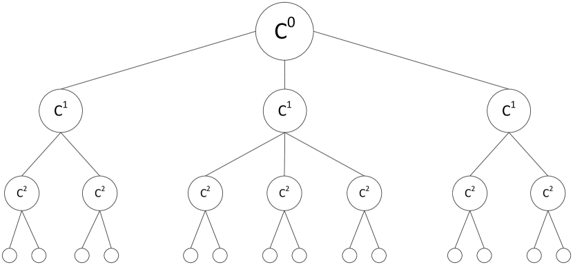
Figure 1: A multi-level network.

Figure 1 shows the multi-level network topology assumed for this protocol; the topology is that of a tree. Each level of the network is connected to the one above through a local collection and broadcast node, which we simply denote as local central node. This node is then a leaf node of the above level, e.g. the nodes denoted as $C^{1}$ are leaf nodes of the level $l_{0}$, while being the local central nodes at each of the locations of $l_{1}^{i}$, which for ease of notation we denote solely as $l_{1}$. We assume that there can be at most $\beta$ nodes connected to every central node, meaning that the bound of every channel should be $\beta$.

The goal of the distributed protocol is to collect information from all leaf nodes in the network; and then communicate it to a central entity, denoted as $C^{0}$. The central entity $C^{0}$, then reaches a global decision, which is then communicated to the leaf nodes. For simplicity, we assume that this decision only depends on the data collected from the leaves.

5.1 The $n$-level protocol in BBC

In what follows, we define the components of the network and protocol inductively. We assume the network to have $n$ levels or depth $n$, where level $0$ corresponds to the central entity, while level $n$ denotes the level where all the leaf nodes are.

One of the sub-networks of the $n$-level protocol at level $k$ , as depicted in Figure 1, is composed by $m$ nodes and a local central node $C_{k}$. We denote this sub-network by the agent identifier $D^{k,n}\left(a^{\prime}_{k},a^{\prime\prime}_{k},b^{\prime}_{k},b^{\prime\prime}_{k},\mathcal{L},\ell_{k-1}\right)$ where $\mathcal{L}$ is a set of locations and $\ell_{k-1}$ is the local central location at $k-1$ level. The other name parameters are

• $a^{\prime}_{k},a^{\prime\prime}_{k}$ - names of the channels used for communications at location $l_{k}$, i.e. between the leaf nodes and the local central entity; the names transmitted are collected by the central node at level $k+1$.

• $b^{\prime}_{k},b^{\prime\prime}_{k}$ - names of the channels that the local central entity uses to communicate to the local central entity for which it is a lead, i.e. the channel over which the local central entity $C_{k}$ communicates with the local central entity $C_{k-1}$. The names transmitted are broadcast to the child nodes of the local central (at level $k-1$).

• $\mathcal{L}$ is the set of nodes at this level.

At the leaf level, $k=0$ we have,

$$D^{0,n}(a^{\prime}_{0},a^{\prime\prime}_{0},b^{\prime}_{0},b^{\prime\prime}_{0}\mathcal{L},\ell_{0}) \stackrel{{\scriptstyle\mathrm{def}}}{{=}}\prod_{\ell_{i}\in\mathcal{L}}\ell_{i}[P_{i}(a^{\prime}_{0},a^{\prime\prime}_{0})]\mid\prod_{\ell_{i}\in\mathcal{L}}\ell_{i}\triangleright\ell_{1}\mid\ell_{0}[C^{0}(a^{\prime}_{0},a^{\prime\prime}_{0},b^{\prime}_{0},b^{\prime\prime}_{0})]$$

The subprocess $P_{i}$ where $\ell_{i}\in\mathcal{L}$ is defined by

$$P_{i}(a^{\prime}_{0},a^{\prime\prime}_{0})\stackrel{{\scriptstyle\mathrm{def}}}{{=}}(\nu\omega_{i}){\overline{a^{\prime}_{0}}}\langle\omega_{i}\rangle.a^{\prime\prime}_{0}(z).(Q_{i}(z)\mid P_{i}(a^{\prime}_{0},a^{\prime\prime}_{0}))$$

where $Q_{i}(z)$ depicts the computation that occurs at the leaf $\ell_{i}$; we shall not describe this here and $\omega_{i}$ is the local name that is the contribution made by the process.

The local central node is defined by

$$C^{0,n}(a^{\prime},a^{\prime\prime},b^{\prime},b^{\prime\prime})\stackrel{{\scriptstyle\mathrm{def}}}{{=}}a^{\prime}(S).{\overline{b^{\prime}}}\langle f(S)\rangle.b^{\prime\prime}(z).{\overline{a^{\prime\prime}}}\langle z\rangle.C^{0,n}(a^{\prime},a^{\prime\prime},b^{\prime},b^{\prime\prime})$$

This process will receive names that are collected to the set $S$ and then pass the processed information $f(S)$ upwards on the $b$ channel. After this, the local central node waits for a response to the information sent and passes on the received name to its children.

The selection function $f:\mathcal{P}(\mathcal{N})\rightarrow\mathcal{N}$ processes the messages received from the leaf nodes and selects a name; this could be e.g. a channel estimate. We require that selection is idempotent in the sense that for any family of multisets $S_{1},\ldots,S_{k}$ we have

$$f(\{f(S_{1}),\ldots,f(S_{k})\})=f(\cup^{k}_{i=1}S_{i})$$

If we think of names as natural numbers, the function $f(S)=\min_{x\in S}x$ is an example of an idempotent selection function.

For intermediate levels, $0<k<n$, $D^{k}\left(a_{k},b_{k},\ell_{k},\ell_{k-1}\right)$ is defined as follows,

$$D^{k+1,n}(a^{\prime}_{k+1},a^{\prime\prime}_{k+1},b^{\prime}_{k+1},b^{\prime\prime}_{k+1},\mathcal{L},\ell_{k+1})\stackrel{{\scriptstyle\mathrm{def}}}{{=}}(\nu\vec{\ell},a^{\prime}_{k}:\beta,a^{\prime\prime}_{k}:\beta,b^{\prime}_{k}:\beta,b^{\prime\prime}_{k}:\beta)$$

$$\left(\prod_{\mathcal{L}_{i}\in\mathsf{Locs}(\mathcal{L},k)}D^{k,n}(a^{\prime}_{k},a^{\prime\prime}_{k},b^{\prime}_{k},b^{\prime\prime}_{k},\mathcal{L}_{i},\ell_{i})\mid\right.\left.\prod^{m}_{i=1}\ell_{i}\triangleright\ell_{k}\mid\ell_{k+1}[C^{k+1}(a^{\prime}_{k},a^{\prime\prime}_{k},b^{\prime}_{k},b^{\prime\prime}_{k})]\right)$$

where the set of locations $\mathsf{Locs}(\mathcal{L},k)$ can be partitioned as $\mathsf{Locs}(\mathcal{L},k)=\bigcup_{i}{i\in I}\mathcal{L}_{i}$ where $I$ is some index set and $\mathcal{L}_{i}\cap\mathcal{L}_{j}=\emptyset$ for all $i\neq j,i,j\in I$. $m^{\prime}_{i}$ is the number of neighbours in the $i$’th sub-network found at level $k+1$ and $\ell_{i}\in\vec{\ell}$.

The definition of local central nodes is (for $k<n$)

$$C^{k,n}((a_{k},b_{k})\stackrel{{\scriptstyle\mathrm{def}}}{{=}}a_{k}(S).{\overline{b_{k}}}\langle f(S)\rangle.b_{k}(z).{\overline{a_{k}}}\langle z\rangle.(Q_{c}(z)\!\mid\!C^{k}(a_{k},b_{k}))$$

Finally, at level $n$ the information collected from all the leaf nodes reaches the central entity, where the final processing of the received information is performed. The description of the entire network $D^{n}$ is $D^{n,n}_{m}(a_{0},\ell_{c})$, defined as

$$D^{n,n}(a^{\prime}_{n},a^{\prime\prime}_{n},b^{\prime}_{n},b^{\prime\prime}_{n},\ell_{n})\stackrel{{\scriptstyle\mathrm{def}}}{{=}}(\nu\vec{\ell},a^{\prime}_{n-1}:\beta,a^{\prime\prime}_{n-1}:\beta,b^{\prime}_{n-1}:\beta,b^{\prime\prime}_{n-1}:\beta)$$

$$\left(\prod_{\mathcal{L}_{i}\in\mathsf{Locs}(\mathcal{L},n)}D^{1,n}_{m^{\prime}_{i}}(a^{\prime}_{n-1},a^{\prime\prime}_{n-1},b^{\prime}_{n-1},b^{\prime\prime}_{n-1},\mathcal{L}_{i},\ell_{n})\right.\mid \left.\prod^{m}_{i=1}\ell_{i}\triangleright\ell_{0}\mid\ell_{0}[C^{n}(a^{\prime}_{n},a^{\prime\prime}_{n},b^{\prime}_{n},b^{\prime\prime}_{n})]\right)$$

Here the central entity will collect the estimates from its children and then broadcast back the value of the selection.

$$C^{n,n}(a^{\prime}_{n},a^{\prime\prime}_{n},b^{\prime}_{n},b^{\prime\prime}_{n})\stackrel{{\scriptstyle\mathrm{def}}}{{=}}a^{\prime}_{n}(S).{\overline{b^{\prime}_{n}}}\langle f(S)\rangle.C^{n,n}(a^{\prime}_{n},a^{\prime\prime}_{n},b^{\prime}_{n},b^{\prime\prime}_{n}))$$ (1)

5.2 Correctness

We would like the multi-level network that serves $K$ leaf nodes to be equivalent to a single-level network containing the same $K$ leaf nodes but now connected to a single central entity.

To this end we define the flattened version of a hierarchical network $N$, denoted $\textsf{flat}(N,\ell)$. This is precisely a network in which all nodes are connected to the same central node at location $\ell$.

This operation is defined inductively as follows.

$$\textsf{flat}(D^{0,n}(a^{\prime}_{0},a^{\prime\prime}_{0},b^{\prime}_{0},b^{\prime\prime}_{0},\mathcal{L},\ell_{0}),\ell)\stackrel{{\scriptstyle\mathrm{def}}}{{=}}D^{0,n}(a^{\prime}_{0},a^{\prime\prime}_{0},b^{\prime}_{0},b^{\prime\prime}_{0},\mathcal{L},\ell_{0})$$

$$\textsf{flat}(D^{k+1,n}(a^{\prime}_{k+1},a^{\prime\prime}_{k+1},b^{\prime}_{k+1},b^{\prime\prime}_{k+1},\mathcal{L},\ell_{k+1}),\ell)\stackrel{{\scriptstyle\mathrm{def}}}{{=}}$$

$$(\nu\vec{\ell},a^{\prime}_{k},a^{\prime\prime}_{k},b^{\prime}_{k},b^{\prime\prime}_{k})\left(\prod^{m}_{\mathcal{L}_{i}\in\mathsf{Locs}(\mathcal{L},k)}\textsf{flat}(D^{k,n}(a^{\prime}_{k},a^{\prime\prime}_{k},b^{\prime}_{k},b^{\prime\prime}_{k},\mathcal{L}_{i},\ell_{i}))\mid\prod^{m}_{i=1}\ell_{i}\triangleright\ell\right)\text{where}\;0<k<n$$

Theorem 3.

For every $n\geq 0$, for every set of distinct names $\{a^{\prime}_{0},a^{\prime\prime}_{0},b^{\prime}_{0},b^{\prime\prime}_{0}\}$ and set of locations $\mathcal{L}$ we have

$$D^{0,n}(a^{\prime}_{0},a^{\prime\prime}_{0}.b^{\prime}_{0},b^{\prime\prime}_{0},\mathcal{L},\ell)\stackrel{{\scriptstyle\cdot}}{{\approx}}\textsf{flat}(D^{0,n}(a^{\prime}_{0},a^{\prime\prime}_{0},b^{\prime}_{0},b^{\prime\prime}_{0},\mathcal{L},\ell),\ell)$$

6 A type system

We can formulate a type discipline that distinguishes between broadcast and collection and assigns bounds to these.

Types are given by the formation rules

$$T::=\textsf{Ch}_{\mathsf{C}}(T)\mid\textsf{Ch}_{\mathsf{B}}(T)\mid T^{k}\mid T_{1}\times T_{2}\cdots\times T_{k}\mid T_{1}\rightarrow T_{2}\mid\textsf{Loc}$$

We now explain the intent behind these formation rules.

• The type $\textsf{Ch}_{\mathsf{C}}(T)$ is the type of a channel than can collect messages of type $T$, and the type $\textsf{Ch}_{\mathsf{B}}(T)$ is the type of a channel that can broadcast a message of type $T$.

• A multiset with $k$ elements of type $T$ will have type $T^{k}$.

• A tuple with $k$ components of types $T_{1},\ldots,T_{k}$, respectively, will have type $T_{1}\times\cdots\times T_{k}$

• A constructor $f$ will have type $T_{1}\rightarrow T_{2}$, and a multiset $g$ will have type $T^{k}\rightarrow T$. If $g$ has type $T^{k}\rightarrow T$, $g$ produces an element of type $T$ from a multiset of $k$ terms, each having type $T$.

• Locations have type Loc.

A type environment $\Gamma$ is a finite function $\Gamma:\textbf{Names}\cup\textbf{Sels}\cup\textbf{Cons}\rightarrow\textbf{Types}$ that assigns types to all names, term constructors and multiset selectors.

Type judgments are relative to a type environment and a set of agent variables $\Theta$ and are of the form

$$\Gamma\vdash M:T$$ for terms

$$\Gamma\vdash^{\Theta}P$$ for processes

$$\Gamma\vdash^{\Theta}N$$ for networks

When the set is the same in all the judgements of a type rule, we omit it throughout the rule.

(Var)	$\Gamma\vdash x:T$ if $\Gamma(x)=T$	(SetVar)	$\Gamma\vdash S:T^{k}$ if $\Gamma(S)=T^{k}$
(Multiset)	$$\frac{\Gamma\vdash M_{i}:T\quad 1\leq i\leq k}{\Gamma\vdash\{M_{1},\ldots,M_{k}\}:T^{k}}\hskip 14.22636pt$$	(Select)	$$\frac{E:T^{k}\quad\Gamma(g)=T^{k}\rightarrow T}{\Gamma\vdash g(E):T}\hskip 14.22636pt$$
(Cons)	$$\frac{\Gamma\vdash M:T_{1}\quad\Gamma(f)=T_{1}\rightarrow T_{2}}{\Gamma\vdash f(M):T_{2}}\hskip 14.22636pt$$

Table 6: Type rules for message terms

(B-Inp)	$$\frac{\Gamma,\vec{x}:\vec{T}\vdash M:T_{1}\quad\Gamma(a)=\textsf{Ch}_{\mathsf{B}}(T_{1})\quad\Gamma,\vec{x}:\vec{T}\vdash P_{1}}{\Gamma\vdash a\,(\lambda\vec{x}M\,)P_{1}}\hskip 14.22636pt$$
(C-Inp)	$$\frac{\Gamma,\vec{x}:\vec{T}\vdash M:T_{1}\quad\Gamma(a)=\textsf{Ch}_{\mathsf{C}}(T_{1})\quad\Gamma,\vec{x}:\vec{T}\vdash P_{1}}{\Gamma\vdash a\,[\lambda\vec{x}M.S\,]P_{1}}\hskip 14.22636pt$$
(Outp)	$$\frac{\Gamma(a)=\textsf{Ch}_{\mathsf{d}}(T)\quad\mathsf{d}\in\{\mathsf{B},\mathsf{C}\}\quad\Gamma\vdash M:T_{1}}{\Gamma\vdash{\overline{a}}\langle M\rangle.P_{1}}\hskip 14.22636pt$$
(Nil)	$\Gamma\vdash\mathbf{0}$	(Par)	$$\frac{\Gamma\vdash P_{1}\quad\Gamma\vdash P_{2}}{\Gamma\vdash P_{1}\mid P_{2}}\hskip 14.22636pt$$
(Sum)	$$\frac{\Gamma\vdash P_{1}\quad\Gamma\vdash P_{2}}{\Gamma\vdash P_{1}+P_{2}}\hskip 14.22636pt$$	(Match)	$$\frac{\Gamma\vdash M_{1}:T\quad\Gamma\vdash M_{2}:T\quad\Gamma\vdash P_{1}}{\Gamma\vdash[M_{1}=M_{2}]P_{1}}\hskip 14.22636pt$$
(Mismatch)	$$\frac{\Gamma\vdash M_{1}:T\quad\Gamma\vdash M_{2}:T\quad\Gamma\vdash P_{1}}{\Gamma\vdash[M_{1}\neq M_{2}]P_{1}}\hskip 14.22636pt$$	(New)	$$\frac{\Gamma,x:T\vdash P_{1}}{\Gamma\vdash(\nu x:\beta_{n})P_{1}}\hskip 14.22636pt$$
(Agent)	$$\frac{\Gamma\vdash M_{i}:T_{i}\quad 1\leq i\leq|\vec{M}|\quad A\in\Theta}{\Gamma\vdash^{\Theta}A(\vec{M})}\hskip 14.22636pt$$
(Call)	$$\frac{\Gamma,\vec{x}:\vec{T}\vdash^{\Theta\cup\{A\}}\vdash P\quad\Gamma\vdash M_{i}:T_{i}\quad 1\leq i\leq|\vec{M}|\quad A(\vec{x})\stackrel{{\scriptstyle\mathrm{def}}}{{=}}P}{\Gamma\vdash^{\Theta}A(M)}\hskip 14.22636pt$$

Table 7: Type rules for processes

(Par-N)	$$\frac{\Gamma\vdash N_{1}\quad\Gamma\vdash N_{2}}{\Gamma\vdash N_{1}\mid N_{2}}\hskip 14.22636pt$$
(New)	$$\frac{\Gamma,x:T\vdash N_{1}}{\Gamma\vdash(\nu x:\beta_{n})N_{1}}\hskip 14.22636pt$$
(Loc)	$$\frac{\Gamma\vdash P\quad\Gamma(\ell)=\textsf{Loc}}{\Gamma\vdash l[P]}\hskip 14.22636pt$$
(Near)	$$\frac{\Gamma(l)=\textsf{Loc}\quad\Gamma(m)=\textsf{Loc}}{\Gamma\vdash l\triangleright m}\hskip 14.22636pt$$
(Not-Near)	$$\frac{\Gamma(l)=\textsf{Loc}\quad\Gamma(m)=\textsf{Loc}}{\Gamma\vdash l\not\triangleright\,m}\hskip 14.22636pt$$

Table 8: Type rules for networks

The following result, which guarantees that a well-typed network stays well-typed under reductions, is easily established.

Theorem 4.

If $\Gamma\vdash N$ and $N\rightarrow N^{\prime}$ then $\Gamma\vdash N^{\prime}$

Proof.

Induction in the reduction rules. A crucial lemma needed in the proof is that whenever $N_{1}\equiv N_{2}$, then $\Gamma\vdash N_{1}$ if and only if $\Gamma\vdash N_{2}$. ∎

7 The expressive power of BBC

There is no compositional encoding of BBC into the $\pi$-calculus. In the presence of broadcast this follows from the negative result due to Ene and Muntean [1]. However, the result also holds if we only consider collection. The following criteria for compositionality are due to Palamidessi [6] and Ene and Muntean [1].

Definition 4.

An encoding $[\![\quad]\!]$ is compositional if

1. $[\![N_{1}\mid N_{2}]\!]=[\![N_{1}]\!]\mid[\![N_{2}]\!]$.

2. For any substitution $\sigma$ we have $[\![N\sigma]\!]=[\![N]\!]\sigma$

3. If $N\rightarrow^{*}N^{\prime}$ then $[\![N]\!]\rightarrow^{*}[\![N^{\prime}]\!]$.

4. If $[\![N]\!]\rightarrow^{*}M$ then $[\![N]\!]\rightarrow^{*}M\rightarrow^{*}[\![N^{\prime}]\!]$ for some $N^{\prime}$.

A central notion in the study of process calculi is that of an electoral system. This is a network in which the participants perform a computation that elects a unique leader. Following [6, 1], our definition assumes a network in which the names used are the ‘natural names’ that represent the identity of the $n$ processes in the network.

Definition 5 (Electoral system).

A network $N=P_{1}\mid\cdots\mid P_{n}$ is an electoral system if for every computation $C$, there exists an extension $C^{\prime}$ of $C$, and an index $k\in\{1,\ldots,n\}$ such that for every $i\in\{1,\ldots,n\}$ the projection $C^{\prime}_{i}$ contains exactly one output action of the form $k$ and any trace of a $P_{i}$ may contain at most one action of the form $\overline{l}$ with $l\in\{1,\ldots,n\}$.

We now describe such a system in BBC. The system uses a common channel $a$ whose bound is $n$, where $n$ is the number of principals. The idea is to collect names until $n$ sets of names have been collected. The first to do so sends out a success announcement to everyone in the form of a name $\textsf{chosen}(m)$; the collection function $g(S)$ is defined to select the name with the minimal index among the names of $S$ unless $S$ contains one or more occurrences of a name of the form $\textsf{chosen}(m^{\prime})$ for some $m$. Thus, the first component to receive sufficiently many names from all other components chooses the leader.

Our network is of the form

$$N=\prod^{n}_{i=1}l[l_{i}]{P_{i}}\mid\prod^{n}_{i=1}\prod^{m}_{j=1,j\neq i}l_{i}\triangleright l_{j}$$

We define the $n$ components as follows:

$$P_{i}\stackrel{{\scriptstyle\mathrm{def}}}{{=}} {\overline{a}}\langle i\rangle.a\,[\lambda x.S_{1}\,]\ldots a\,[\lambda x.S_{k}\,]{\overline{a}}\langle\textsf{chosen}(g(\{\{g(S_{1}),\ldots g(S_{k})\}\}))\rangle.P$$

The selection function is defined by

$$g(S)=\begin{cases}\min_{x\in S}x&\text{if}\;S\subseteq\{1,\ldots,n\}\\ \textsf{chosen}(n)&\text{if}\;\textsf{chosen}(n)\in S\end{cases}$$

As there is no such electoral system for the $\pi$-calculus [6], we can use the same proof as that given by Ene and Muntean to conclude that there can be no compositional encoding of BBC in the $\pi$-calculus.

8 Directions for further work

In this paper we have presented the BBC calculus, which is a distributed process calculus that generalizes the $\pi$-calculus with notions of channels with bounded forms of broadcast and collection and an explicit notion of connectivity.

The present work only considers barbed bisimulation; it is well-known that this relation is not preserved by parallel composition and that the notion of barbed congruence does not lend itself well to coinductive proof techniques. Further work includes finding a labelled characterization of barbed congruence; this requires a labelled transition semantics in the spirit of [1].

At present, we informally distinguish between channels for broadcast and collection. However, if we think of channels as radio frequencies, one would sometimes like the same frequency to be used for both broadcast and collection. An interesting direction of work is therefore to develop a type system that will allow the same channel to be used non-uniformly in both modes and according to a protocol. This is a variant of binary session types [2] that has been adapted to a setting with broadcast communication by [5]. A further step in this direction is to study multiparty session types [3] and how the projection to local session types can be defined in the setting of BBC.

References

• [1] Cristian Ene and Traian Muntean. A broadcast-based calculus for communicating systems. In Proceedings of IPDPS’1. IEEE Computer Society, 2001. 10.1007/3-540-48321-7_21
• [2] Kohei Honda, Vasco Thudichum Vasconcelos, and Makoto Kubo. Language primitives and type discipline for structured communication-based programming. In ESOP, volume 1381 of LNCS, pages 122–138. Springer, 1998. 10.1007/BFb0053567
• [3] Kohei Honda, Nobuko Yoshida, and Marco Carbone. Multiparty asynchronous session types. In George C. Necula and Philip Wadler, editors, POPL, pages 273–284. ACM, 2008. 10.1145/1328438.1328472
• [4] Dimitrios Kouzapas and Anna Philippou. A process calculus for dynamic networks. In Roberto Bruni and Juergen Dingel, editors, Formal Techniques for Distributed Systems, volume 6722 of Lecture Notes in Computer Science, pages 213–227. Springer Berlin Heidelberg, 2011. 10.1007/978-3-642-21461-5_14
• [5] Dimitrios Kouzapas and Ramunas Gutkovas and Simon J. Gay. Session Types for Broadcasting In Alastair F. Donaldson and Vasco T. Vasconcelos. Proceedings 7th Workshop on Programming Language Approaches to Concurrency and Communication-cEntric Software, PLACES 2014, Grenoble, France, 12 April 2014, pages 25–31. 10.4204/EPTCS.155.4
• [6] Catuscia Palamidessi. Comparing the expressive power of the synchronous and asynchronous pi-calculi. MSCS, 13(5):685–719, 2003. 10.1017/S0960129503004043
• [7] K. V. S. Prasad. A calculus of broadcasting systems. Sci. Comput. Prog., 25(2-3):285–327, 1995. 10.1016/0167-6423(95)00017-8
• [8] James Riely and Matthew Hennessy. A typed language for distributed mobile processes (extended abstract). In POPL, pages 378–390, 1998. 10.1145/268946.268978
• [9] Davide Sangiorgi and David Walker. The $\pi$-Calculus: A Theory of Mobile Processes, Cambridge University Press, 2001. ISBN 978-0-521-78177-0.
• [10] Anu Singh, C. R. Ramakrishnan, and Scott A. Smolka. A process calculus for mobile ad hoc networks. Science of Computer Programming, 75(6):440–469, 2010. 10.1016/j.scico.2009.07.008