Generating Discriminative Object Proposals via Submodular Ranking

Abstract

A multi-scale greedy-based object proposal generation approach is presented. Based on the multi-scale nature of objects in images, our approach is built on top of a hierarchical segmentation. We first identify the representative and diverse exemplar clusters within each scale by using a diversity ranking algorithm. Object proposals are obtained by selecting a subset from the multi-scale segment pool via maximizing a submodular objective function, which consists of a weighted coverage term, a single-scale diversity term and a multi-scale reward term. The weighted coverage term forces the selected set of object proposals to be representative and compact; the single-scale diversity term encourages choosing segments from different exemplar clusters so that they will cover as many object patterns as possible; the multi-scale reward term encourages the selected proposals to be discriminative and selected from multiple layers generated by the hierarchical image segmentation. The experimental results on the Berkeley Segmentation Dataset and PASCAL VOC2012 segmentation dataset demonstrate the accuracy and efficiency of our object proposal model. Additionally, we validate our object proposals in simultaneous segmentation and detection and outperform the state-of-art performance.

I Introduction

Object recognition has long been a core problem in computer vision. Recent developments in object recognition provide two effective solutions: 1) sliding-window-based object detection and localization [32, 8, 12], 2) segmentation-based approaches [5, 30, 10, 3]. The sliding window approach incurs high computational cost as it analyses windows over a very large set of locations and scales. Segmentation-based methods lead to fewer regions to consider and to better spatial support for objects of interest with richer shape and contextual information; but the problem of segmenting an image to identify regions with high object spatial support is a challenge.

To improve object spatial support and speed up object localization for object recognition, generating high-quality category-independent object proposals as the input for object recognition system has drawn attention recently [10, 30, 7, 3]. Motivated by findings from cognitive psychology and neurobiology [29, 33, 9, 21] that the human vision system has the amazing ability to localize objects before recognizing them, a limited number of high-quality and category-independent object proposals can be generated in advance and used as inputs for many computer vision tasks. This approach has played a dominant role in semantic segmentation [2, 4] and leads to competitive performance on detection [13]. There are two main categories of object proposal generation methods depending on the shape of proposals: bounding-box-based proposals [36, 7, 30] and segment-based proposals [3, 10, 28].

Objects in an image are intrinsically hierarchical and of different scales. Consider the table in Figure 1(a) for example. The objects on the table can be regarded as a part of the table (Figure 1(b)), and at the same time, they constitute a group of objects on the table (Figure 1(c)). More specifically, these objects include plates, forks, the Santa Claus, and a bottle (Figure 1(d)). Therefore, multi-scale segmentation is essential to localize and segment different objects. There have been a few attempts [5, 10, 3] to combine multiple scale information in the object proposal generation process, but very few papers have studied the importance of proposal selection given segments from hierarchical image segmentations. Figure 1(e)1(f)1(g) show the generated proposals from three state-of-art algorithms [5, 10, 3]. However, they do not cover all the objects in the image well.

(a) Input

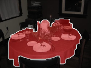
(b) Coarse layer sample

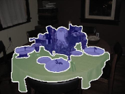
(c) Middle layer samples

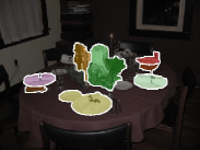
(d) Fine layer samples

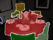
(e) CPMC [5]

(f) Categ. Indep. [10]

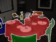
(g) MCG [3]

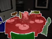
(h) Our method

Figure 1: Objects in an image are naturally hierarchical. (a) is an original image from Pascal VOC2012; (b) - (d) show segments around the table from different scales using method [5]; (e) shows the best seven object proposals generated from CPMC [5]; (f) are proposals from Categ. Indep. [10]; (g) are proposals from MCG [3]; (h) are proposals from our method.

We present a greedy approach to efficiently extract high-quality object proposals from an image via maximizing a submodular objective function. We first construct diverse exemplar clusters of segments over a range of scales using diversity ranking; then rank and select high-quality object proposals from the multi-scale segment pool generated by hierarchical image segmentation. Our objective function is composed of three terms: a weighted coverage term, a single-scale diversity term and a multi-scale reward term. The first term encourages the selected set to be compact and well represent all segments in an image. The second term enforces the selected segments (object proposals) to be diverse and cover as many different objects as possible. The third term encourages the selected proposals to correspond to objects with high confidence and selected from different scales. The algorithm takes object scale information into account and avoids selecting segments from the same layer repeatedly. Compared to existing segment-based methods, our method (Figure 1(h)) can select representative, diverse and discriminative object proposals from different layers (for example, the bottle from fine layer and the table from coarse layer). Our main contributions are as follows:

• The generation of object proposals is solved by maximizing a submodular objective function. An efficient greedy-based optimization algorithm with guaranteed performance is presented based on the submodularity property.

• We naturally integrate multi-scale and object discriminativeness information into the objective function. The generated proposals are representative, diverse and discriminative.

• Our approach achieves state-of-the-art performance on two popular datassets, and our generated object proposals, when integrated into simultaneous segmentation and detection, achieves state of the art results.

II Related work

The goal of object proposal algorithms is to generate a small number of high-quality category-independent proposals such that each object in an image is well captured by at least one proposal [1, 10]. Existing object proposal approaches can be roughly divided into bounding-box and segment based approaches. [36] generated bounding boxes by utilizing edge and contour clues. In [30], a data-driven grouping strategy which combines segmentation and exhaustive search is presented to produce bounding-box-based proposals. [7] proposed the binarized normed gradients (BING) feature to efficiently produce object boxes. Instead of generating bounding-box-based proposals, our work focuses on extracting segment-based proposals which aims to cover all the objects in an image and can provide more accurate shape and location information. Some algorithms have been reported to generate segment-based object proposals. [5] segmented objects by solving a series of constrained parametric min-cut (CPMC) problems. [17] reused inference in graph cuts to solve the parametric min-cut problems much more efficiently. [10] performed graph cuts and ranked proposals using structured learning. In [3], a hierarchical segmenter is used to combine multi-scale information, and a grouping strategy is presented to extract object candidates. Different from their work, we design an efficient greedy-based ranking method to leverage multi-scale information in the process of selecting object proposals from a large hierarchical segment pool.

Object proposals have been used in many computer vision tasks, such as segmentation [2, 5], object detection [13] and large-scale classification [30]. Semantic segmentation and object detection have been shown to support each other mutually in a wide variety of algorithms. [25] showed that better quality segmentation can improve object recognition performance. [13, 6, 16] used hierarchical segmentations and combined several top-down cues for object detection. The more demanding task of simultaneous detection and segmentation (SDS) is investigated in [16] which detects and labels the segments at the same time. We use this same detection and segmentation framework but with our object proposal generation method to demonstrate the effectiveness of proposals generated by our approach.

Submodular optimization is a useful optimization tool in machine learning and computer vision problems [22, 23, 19, 18, 24, 35]. [22] demonstrates how submodularity speeds up optimization algorithm in large scale problems. In [19], a diffusion-based framework is proposed to solve cosegmentation problems via submodular optimization. [18] used the facility location problem to model salient region detection where salient regions are obtained by maximizing a submodular objective function.

III Submodular Proposal Extraction

We first obtain a large pool of segments from different scales using hierarchical image segmentation. Diverse exemplar clusters are then generated via diversity ranking within each layer to discover potential objects in an image. We define a submodular objective function to rank and select a discriminative and compact subset from a large set of segments of different scales, then the selected segments are used as the final object proposals.

III-A Preliminaries

Submodularity: Let $V$ be a finite set, $A\subseteq B\subseteq V$ and $a\in V\setminus B$. A set function $F:2^{v}\rightarrow R$ is submodular if $F(A\bigcup a)-F(A)\geqslant F(B\bigcup a)-F(B)$. This is the diminishing return property: adding an element to a smaller set helps more than adding it to a larger set [27].

III-B Hierarchical Segmentation

We build our object proposal generation framework on top of hierarchical segmentation. Following [5, 17], we generate segments for an image at different scales by solving multiple constrained parametric min-cut problems with different seeds and unary terms.

III-C Exemplar Cluster Generation

In a coarser layer, an image is segmented into only a few segments. However, the number of segments increases dramatically as we go to finer layers. To reduce the redundancy and maintain segment diversity, we introduce an exemplar cluster generation step to pre-process segments within layers.

Let $V$ denote the set containing segments from all layers of an image (the multi-scale segment pool), and $V^{l}$ be the set of segments from layer $l$. Then $V=\bigcup_{l=1}^{L}V^{l}$, $L$ is the total number of layers, and $V^{l}$s are disjoint. For each layer $l$, we obtain a partition of its segments $\{P_{1}^{l},P_{2}^{l},...,P_{t}^{l}\}$ using a diversity ranking algorithm [19]. $P_{t}^{l}$ is the set of segments assigned to cluster $t$. Each segment belongs to only one cluster, and clusters are disjoint. For each layer $L$, we have $V^{l}=\cup_{t=1}^{T}P_{t}^{l}$, where $T$ is the number of clusters.

III-D Submodular Multi-scale Proposal Generation

We present a proposal generation method by selecting a subset $A$ which contains high-quality segments (object proposals) from the set $V$.

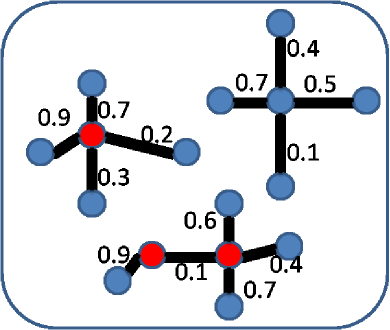
(a) H(A)=7.7

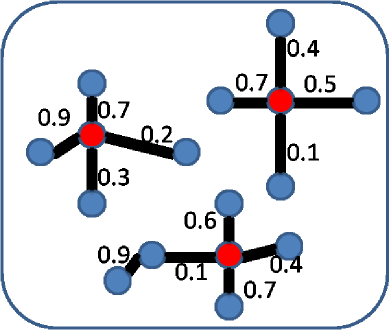
(b) H(A)=8.6

Figure 2: The weighted coverage term for the representative proposal selection (best viewed in color). The node denotes the segment vertex, and the value next to the edge is the similarity between vertices. The red nodes are selected vertices. To select three nodes among all, by computing the weighted coverage term, we favours selecting a more representative set (three center nodes in (b) will lead to higher $H(A)$ than the less representative one since the two nodes are from one group in (a)). Hence the selected $A$ is representative and compact.

Given an image $I$, we construct an undirected graph $G=(V,E)$ for the segment hypotheses in $I$. Each vertex $v\in V$ is an element from the multi-scale segment pool. Each edge $e\in E$ models the pairwise relation between vertices. Two segments are connected if they are overlapping (between layers) or adjoining (within a layer). The weight $w_{ij}$ associated with the edge $e_{ij}$ measures the appearance similarity between vertices $v_{i}$ and $v_{j}$. We extract a CNN feature descriptor [15] for each segment: $X=[x_{1},x_{2},...,x_{|V|}]$. $w_{ij}$ is defined as the Gaussian similarity between two vertices’ feature descriptors.

$$w_{ij}=\begin{cases}exp(-\epsilon d^{2}(x_{i},x_{j})),&\text{if $e_{ij}\in E$}.\\ 0,&\text{otherwise}.\end{cases}$$ (1)

As suggested in [34], we set the normalization factor $\epsilon=1/\sigma_{i}\sigma_{j}$ and the local scale $\sigma_{i}$ is selected by the local statistic of vertex $i$’s neighbourhood. We adopt the simple choice which sets $\sigma_{i}=d(x_{i},x_{M})$ where $x_{M}$ corresponds to the $M$’th closest neighbour of vertex $i$.

III-D1 Weighted Coverage Term

The selected subset $A$ should be representative of the whole set $V$. The similarity of subset $A$ to the whole set $V$ is maximized with a constraint on the size of $A$. Accordingly, we introduce a weighted coverage term for selecting representative proposals.

Let $N_{A}$ denote the number of selected segments. Then the weighed coverage term is formulated as:

$$H(A)=\sum_{i\in V}\max_{j\in A}w_{ij}$$ (2)

$$s.t.\quad A\subseteq V,N_{A}\leqslant K$$

where $K$ is the maximum number of segments to be chosen in set $A$. The weighted coverage of each segment $v_{i}$ is $\max_{j\in A}w_{ij}$. Equation (2) measures the representativeness of $A$ to $V$ and favours selecting segments which can cover (or represent) the other unselected segments. Maximizing the weighted coverage term encourages the selected set $A$ to be representative and compact as shown in Figure 2.

III-D2 Single-Scale Diversity Term

The weighted coverage term will give rise to a highly representative set $A$; however, segments from each layer (corresponding to each image scale) still possess redundancy. Therefore, we introduce a diversity term to force segments within a layer $l$ to be different. The single-layer diversity term is formulated as follows:

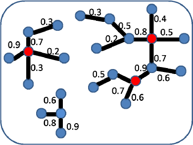
(a) D(A)=0.90

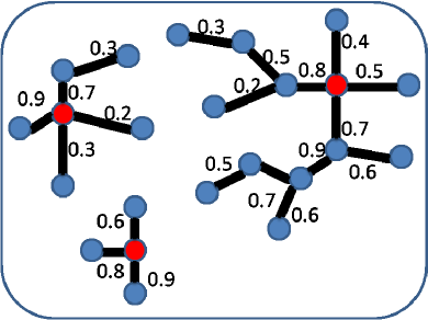
(b) D(A)=1.13

Figure 3: The single-layer diversity term for the diverse proposal selection. Each node denotes a segment vertex (best viewed in color). Similarity between vertices are labelled next to each edge. The red node labels the selected segments. Each figure shows three exemplar clusters as connected groups. We can see the three exemplar clusters are unbalanced. Purely computing the weighted coverage term will pick the third node from the largest cluster to gain more similarity between the selected set and the whole set as in (a). While by computing the single-layer diversity term, we observe that (b) is preferred to (a) as it encourage diversity among the selected nodes.

$$D(A)=\sum_{l=1}^{L}D_{l}(A)=\sum_{t,l}\sqrt{\sum_{j\in P_{t}^{l}\cap A}\frac{1}{|V^{l}|}(\sum_{i\in V^{l}}w_{ij})}$$ (3)

where $P_{t}^{l}$ is the set of segments which belong to cluster $t$ in layer $l$ (defined in section III-C). $|V^{l}|$ is the number of segments in layer $l$. This single-scale diversity term encourages $A$ to include elements from different clusters and leads to more diverse segments from each layer. The single-layer diversity term is submodular; a detailed proof is provided in the supplementary material.

In many images, the background composes a large part of the image. For a single layer, the segments corresponding to objects are only a small percentage of all segments. The segment distributions corresponding to different objects and the background are generally unbalanced. The weighted coverage term favours selecting segments that well represent all segments, resulting in redundancy and occasionally missing small objects. Together with the single-layer diversity term, diversity among the selected segments are enforced as shown in Figure 3.

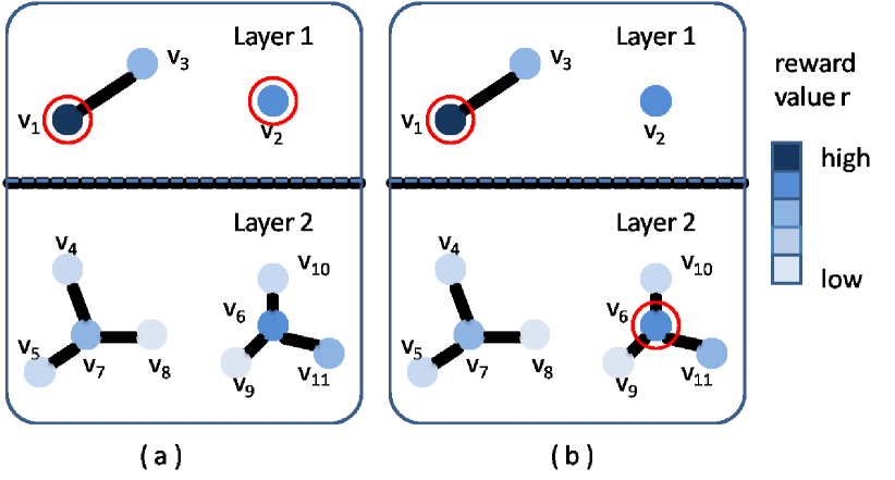
Figure 4: The multi-scale reward term for selecting proposals from different scales (best viewed in color). The nodes represent segments. The reward value $r_{i}$ of segment $v_{i}$ is reflected by color. The higher $r_{i}$, the more likely it is an object. The red circle denotes the selected nodes. Suppose $v_{1}$ has already been selected. We observe that $R\{v_{1},v_{2}\}-R\{v_{1}\}<R\{v_{1},v_{6}\}-R\{v_{1}\}$. In another word, although $v_{2}$ and $v_{6}$ have similar reward value, $v_{6}$ from layer $2$ will brings higher marginal gain; thus $v_{6}$ is favoured over $v_{2}$ and (b) is preferred to (a).

III-D3 Multi-Scale Reward Term

Considering the multi-scale nature of objects in an image, we propose the following discriminative multi-scale reward term to encourage selected segments to have high likelihood of high object coverage. The multi-scale reward term is defined as:

$$R(A)=\sum_{l=1}^{L}\sqrt{\sum_{j\in V^{l}\bigcap A}r_{j}}$$ (4)

$V^{l}$ is the set of segments from layer $l$. The value $r_{j}$ estimates the likelihood of a segment to be an object. It determines the priority of a segment being chosen in its layer. We use CNN features to train a SVM model over object segments and non-object segments in training images and then assign a confidence score for each segment during testing. The confidence score is used as $r_{j}$ for a segment $v_{j}$.

The multi-scale reward term encourages $A$ to select a set of discriminative segments from multi-scale segments generated from a hierarchical segmentation. As soon as an element is selected from a layer, other elements from the same layer start to have diminishing gain because of the submodular property of $R(A)$. A simple example is shown in Figure 4. Similar to $D(A)$, $R(A)$ is submodular and the proof is presented in the supplementary material.

IV Optimization

We combine the weighted coverage term, the single-scale diversity term and the multi-scale reward term to find high-quality object proposals. The final objective function of object proposal generation is formulated as below:

$$\max_{A}F(A) = \max_{A}H(A)+\alpha D(A)+\beta R(A)$$

$$= \max_{A}\sum_{i\in V}\max_{j\in A}w_{ij}+\beta\sum_{l=1}^{L}\sqrt{\sum_{j\in V^{l}\bigcap A}r_{j}}$$

$$+\alpha\sum_{n,l}\sqrt{\sum_{j\in P_{t}^{l}\cap A}\frac{1}{|V^{l}|}(\sum_{i\in V^{l}}w_{ij})}$$

$$s.t.\quad A\subseteq V,N_{A}\leq K,\alpha\geq 0,\beta\geq 0$$

The submodularity is preserved by taking non-negative linear combinations of the three submodular terms $H(A)$, $D(A)$, and $R(A)$. Direct maximization of equation (IV) is an NP-hard problem. We can approximately solve the problem via a greedy algorithm [14, 27] based on its submodularity property. A lower bound of $(e-1)/e$ times the optimal value is guaranteed as proved in [27] (e is the base of the natural logarithm).

	AUC	Recall	BSS
C,T+layout [10]	77.5	83.4	67.2
all feature [10]	80.2	79.7	66.2
Ours	81.1	83.6	71.8

TABLE I: Comparison of object proposals’ quality on the BSDS dataset, measured with AUC, recall and BSS.

The algorithm starts from an empty set $A=\varnothing$. It adds the element $a^{*}$ which provides the largest marginal gain among the unselected elements to $A$ iteratively. The iterations stop when $|A|$ reaches the desired capacity number $K$. The optimization steps can be further accelerated using a lazy greedy approach from [22]. Instead of recomputing gain for every unselected element after each iteration, an ordered list of marginal benefits will be maintained in descending order. Only the top unselected segment is re-evaluated at each iteration. Other unselected segments will be re-evaluated only if the top segment does not remain at the top after re-evaluation. The pseudo code is presented in Algorithm 1.

Algorithm 1 Submodular object proposal generation

Input: $I$, $G=(V,E)$, $K$, $\alpha$, $\beta$

Output: $A$

Initialization: $A\leftarrow\varnothing$, $U\leftarrow V$

loop

     $a^{*}=arg\underset{a\in U}{\max}F(A\cup\{a\})-F(A)$

     if $|A|\geq K$ then

         break      

     $A\leftarrow A\cup\{a^{*}\}$

     $U\leftarrow U-\{a^{*}\}$

V Experiments

We evaluate our approach on two public datasets: BSDS [26] and PASCAL VOC2012 [11] segmentation dataset. The results for PASCAL VOC2012 are on the validation set of the segmentation task. We evaluate the object proposal quality by assessing the best proposal for each object using the Jaccard index score (see details in section V-A). We also compare our ranking method with several baselines [10] and analyses the efficiency of our object proposals on the object recognition task.

Method	N	Plane	Bike	Bird	Boat	Bottle	Bus	Car	Cat	Chair	Cow	Table	Dog	Horse	MBike	Person	Plant	Sheep	Sofa	Train	TV	Global
Ours	1100	82.3	48.8	84.6	76.7	71.4	80.6	67.7	93.1	69.7	86.0	78.5	89.7	83.2	77.3	72.9	70.4	77.8	85.8	85.0	87.5	76.5
[3]	1100	80.0	47.8	83.9	76.4	71.1	78.5	68.9	89.3	68.5	85.9	79.8	85.8	80.4	75.4	73.5	69.3	84.9	82.6	81.7	85.8	76.0
[10]	1100	75.1	49.1	80.7	68.8	62.8	76.4	63.3	89.4	64.6	83.0	80.3	83.7	78.4	78.0	66.9	66.2	69.5	82.0	84.3	81.8	71.6
[2]	1100	74.4	46.6	80.5	69.4	64.6	73.5	61.2	89.0	65.1	80.5	78.4	85.2	77.2	70.6	67.9	68.8	73.5	81.6	75.8	82.0	71.4
[20]	1100	73.8	40.6	75.8	66.7	52.7	79.7	50.6	91.2	59.2	80.2	80.7	87.4	79.0	74.7	62.1	54.6	65.0	84.6	82.4	79.5	67.4
[31]	1100	68.3	39.6	70.6	64.8	58.0	68.2	51.8	77.6	58.2	72.6	70.4	74.0	66.2	59.9	59.8	55.4	67.7	71.3	68.6	78.7	63.1
ours	100	75.2	40.8	78.4	70.3	55.5	72.8	51.1	83.4	56.8	77.3	66.7	84.4	75.2	65.9	59.3	54.9	68.1	77.9	76.1	76.8	64.3
[3]	100	70.2	38.8	73.6	67.7	55.3	68.5	50.6	82.4	54.4	78.1	67.7	77.7	69.3	66.3	59.9	51.4	70.2	74.1	72.6	78.1	63.7
[10]	100	70.6	40.8	74.8	59.9	49.6	65.4	50.4	81.5	54.5	74.9	68.1	77.3	69.3	66.8	56.2	54.3	64.1	72.0	71.6	69.9	61.7
[5]	100	72.7	36.2	73.6	63.3	45.4	67.4	39.5	84.1	47.7	73.2	64.0	81.1	72.2	64.3	52.8	42.9	62.2	72.9	74.3	69.5	59.0

TABLE II: VOC2012 val set. Jaccard index at the instance level and class level.

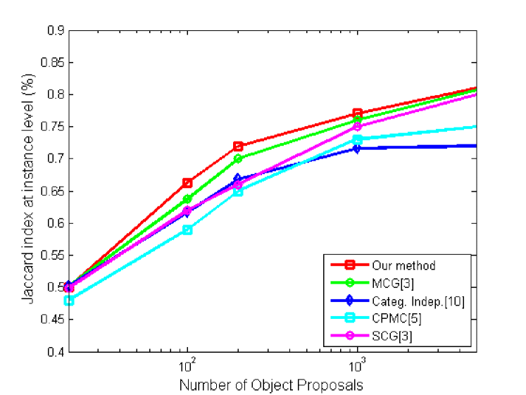
Figure 5: Object proposal quality on PASCAL VOC2012 validation set, measured with the Jaccard index at instance level $J_{i}$.

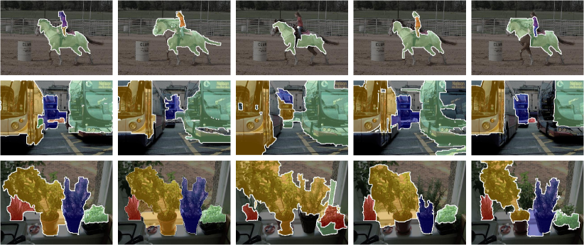
Figure 6: Sample object proposals from the PASCAL VOC2012. The left column shows the best four proposals for objects in our model. The remaining columns show the highest ranked proposals with at least 50 percent overlap with an object. The second column is from our method, the third column is from Categ. Indep. [10], the fourth column is from CPMC [5], and the last column is from MCG [3].

V-A Proposal evaluation

To measure the quality of a set of object proposals, we followed [3] and compute the Jaccard index score, or the best segmentation overlap score (BSS) for each object. The overall quality of a object proposal set is measured at the class level and the instance level. The Jaccard index at instance level, denoted as $J_{i}$, is defined as the mean of BSS over all objects. The Jaccard index at class level, $J_{c}$ is defined as the mean of BSS over objects from each category.

V-A1 BSDS dataset

We compare our object proposals with [10]. For fair comparison, we also compute the area under the ROC curve (AUC) and recall defined with an overlap threshold at 50 per cent. The results are summarized in Table I. Our object proposal achieves the best performance.

V-A2 PASCAL VOC2012

Method	Plane	Bike	Bird	Boat	Bottle	Bus	Car	Cat	Chair	Cow	Table	Dog	Horse	MBike	Person	Plant	Sheep	Sofa	Train	TV	Mean
O2P [16]	56.5	19.0	23.0	12.2	11.0	48.8	26.0	43.3	4.7	15.6	7.8	24.2	27.5	32.3	23.5	4.6	32.3	20.7	38.8	32.3	25.2
SDS-A [16]	61.8	43.4	46.6	27.2	28.9	61.7	46.9	58.4	17.8	38.8	18.6	52.6	44.3	50.2	48.2	23.8	54.2	26.0	53.2	55.3	42.9
SDS-B [16]	65.7	49.6	47.2	30.0	31.7	66.9	50.9	69.2	19.6	42.7	22.8	56.2	51.9	52.6	52.6	25.7	54.2	32.2	59.2	58.7	47.0
SDS-C [16]	67.4	49.6	49.1	29.9	32.0	65.9	51.4	70.6	20.2	42.7	22.9	58.7	54.4	53.5	54.4	24.9	54.1	31.4	62.2	59.3	47.7
Ours	68.2	14.0	64.7	51.3	39.3	62.1	45.6	65.8	9.9	49.1	30.8	61.9	54.9	65.9	54.5	31.8	48.4	29.5	73.9	65.6	48.9

TABLE III: Results on AP^r on the PASCAL VOC2012 val. All numbers are $\%$.

We evaluate our object proposal approach on the PASCAL VOC2012 validation dataset. The SVM classifier for reward value (details in section III-D3) is trained on the training dataset. Our object proposals are compared with [20, 5, 2, 31, 10, 3]. As shown in Table II, our method outperform all other methods with the same number of object proposals for Jaccard index at the instance level. Meanwhile, we achieve the highest scores on most of the classes (14 out of 20). In Figure 5, we show how $J_{i}$ changes as the number of object proposals increases. Since our approach prefers to select representative, diverse and multi-scale object proposals, our proposal quality outperform MCG [3], Categ. Indep. [10], CPMC [5], and SCG [3] with only a small number of proposals. In Figure 6, we show some qualitative results of our object proposals. We observe that our proposals can capture diverse objects of different sizes. In addition, we compare our proposal generation time with MCG [3] which also uses multi-scale information. Our method takes about 7 seconds per image compared to 10 seconds reported in [3]. The parameters are set $\alpha=3.9$, $\beta=2.0$ in our experiments.

Method	Plane	Bike	Bird	Boat	Bottle	Bus	Car	Cat	Chair	Cow	Table	Dog	Horse	MBike	Person	Plant	Sheep	Sofa	Train	TV	Mean
O2P [16]	46.8	21.2	22.1	13.0	10.1	41.9	24.0	39.2	6.7	14.6	9.9	24.0	24.4	28.6	25.6	7.0	29.0	18.8	34.6	25.9	23.4
SDS-A [16]	48.3	39.8	39.2	25.1	26.0	49.5	39.5	50.7	17.6	32.5	18.5	46.8	37.7	41.1	43.2	23.4	43.0	26.2	45.1	47.7	37.0
SDS-B [16]	51.1	42.1	40.8	27.5	26.8	53.4	42.6	56.3	18.5	36.0	20.6	48.9	41.9	43.2	45.8	24.8	44.2	29.7	48.9	48.8	39.6
SDS-C [16]	53.2	42.1	42.1	27.1	27.6	53.3	42.7	57.3	19.3	36.3	21.4	49.0	43.6	43.5	47.0	24.4	44.0	29.9	49.9	49.4	40.2
SDS-C+ref [16]	52.3	42.6	42.2	28.6	28.6	58.0	45.4	58.9	19.7	37.1	22.8	49.5	42.9	45.9	48.5	25.5	44.5	30.2	52.6	51.4	41.4
Ours	54.7	19.4	54.3	40.9	34.4	52.0	41.3	59.3	13.3	42.9	25.8	51.9	44.8	51.5	47.0	31.4	42.6	28.5	59.2	53.8	42.4

TABLE IV: Results on AP${}^{r}_{vol}$ on the PASCAL VOC2012 val. All numbers are $\%$.

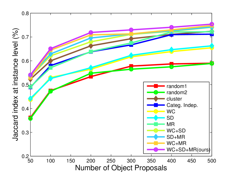
Figure 7: Comparing different ranking methods (random selection, clustering, Categ. Indep. [10], WC, SD, MR, WC+SD, WC+MR, SD+MR, WC+SD+MR(ours)).

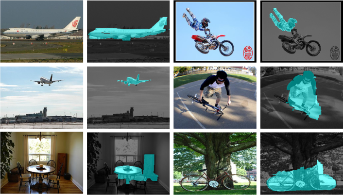
Figure 8: Top detections on: aeroplane, person, dining table, bicycle.Our detection results work well on objects of different scales.

V-B Ranking performance

To explore our method’s ranking ability, we compare our ranking method with four baselines on the PASCAL VOC2012 dataset. 1) Random1 randomly selects object proposals from the multi-scale segment pool. 2) Random2 randomly selects object proposals from each layer evenly, and combine them together. 3) Clustering selects the object proposals which are closest to the cluster center based on euclidean distance. The cluster centres are obtained via k-means clustering and k is set to be the number of object proposals to be selected. 4) Categ. Indep. is the method from [10] to rank segments. In order to show the importance of each term in our model, we evaluate each term: the weighted coverage term(WC), the single-layer diversity term (SD), and the multi-scale reward term (MR). Results of different term combinations (WC+SD, WC+MR, SD+MR) and the full model (WC+SD+MR) are also presented.

Figure 7 shows the quality of the selected object proposals using different ranking methods from the same segment pool. The two random selection methods achieve similar object proposal qualities. Comparing WC, SD and MR terms independently, WC achieves lower quality than the other two. As discussed in III-D1, it emphasize the representativeness of the selected set regardless of whether the segment is an object or not. The clustering method also has the same weakness. The MR term is comparable to structured learning as it also takes into account multi-scale information. Adding the MR term to each of the WC and SD terms increases performance as it introduces discriminative information into the proposal selection process. Our full ranking model selects the best object proposals amongst all.

V-C Semantic Segmentation and Object Detection

To analyse the utility of the object proposals generated by our approach in real object recognition tasks, we perform semantic segmentation and object detection on the PASCAL VOC2012 validation set. We follow the settings in [16], where 2000 object proposals are generated for each image using our algorithm. Then we extract CNN features for both the regions and their bounding boxes using the deep convolutional neural network model pre-trained on ImageNet and fine-tuned on the PASCAL VOC2012 training set, the same as in [16]. These features are concatenated, then passed through linear classifiers trained for region and box classification tasks. After non-maxima suppression, we select the top 20,000 detections for each category.

The results are evaluated with the traditional bounding box AP^b and the extended metric AP^r as in [16] (the superscripts $b$ and $r$ correspond to region and bounding box). The AP^r score is the average precision of whether a hypothesis overlaps with the ground-truth instance by over $50\%$, and the AP${}^{r}_{vol}$ is the volume under the precision recall (PR) curve, which are suitable for the simultaneous segmentation and detection task. The evaluation of the detection task uses $AP^{b}$ and $AP^{b}_{vol}$, which are conventional evaluation metric for object detection.

Table III and Table IV shows the AP^r and AP${}^{r}_{vol}$ results for each class. We can see that the results using our object proposals, both our mean AP^r and mean AP${}^{r}_{vol}$ have achieved state of the art using a seven-layer network, and we outperform previous methods in 14 out of 20 classes. In contrast to SDS [16], we neither fine tune different networks for regions and boxes nor refine the regions after classification. But our results still not only outperform the corresponding SDS-A but also the complicated SDS-B and SDS-C methods which finetuned two networks separately and as a whole. Moreover, on the more meaningful measurement of AP${}^{r}_{vol}$ shown in Table IV, results based on our object proposals even outperform that of SDS-C+ref, where the segments are refined within their $10\times 10$ grid using a pretrained model with class priors. It shows the importance of good quality regions even before carefully designed feature extraction and region refinement after classification.

Table V shows the mean AP^b and mean AP${}^{b}_{vol}$ results for object detection. We achieved better results than RCNN [15], RCNN-MCG [16] and SDS-A [16], which shows that better region proposals not only improve segmentation but also give better localization of objects. Figure 8 shows some examples of our detection results.

	RCNN	RCNN-MCG	SDS-A	Ours
mean APb	51.0	51.7	51.9	52.4
mean AP${}^{b}_{vol}$	41.9	42.4	43.2	44.3

TABLE V: Results on AP^b and AP${}^{b}_{vol}$ on the PASCAL VOC2012 val. All numbers are $\%$.

VI Conclusion

We presented an efficient approach to extract multi-scale object proposals. Built on the top of hierarchical image segmentation, exemplar clusters are first generated within each scale to discover different object patterns. By introducing a weighted coverage term, a single-scale diversity term and a multi-scale reward term, we define a submodular objective function to select object proposals from multiple scales. The problem is solved using a highly efficient greedy algorithm with guaranteed performance. The experimental results on the BSDS dataset and the PASCAL VOC2012 dataset demonstrate that our method achieves state-of-art performance and is computationally efficient. We further evaluate our object proposals on a simultaneous detection and segmentation task to demonstrate the effectiveness of our approach and outperform the object proposals generated by other methods.

References

- [1] B. Alexe, T. Deselaers, and V. Ferrari. Measuring the objectness of image windows. PAMI, 34:2189–2202, 2012.
- [2] P. Arbelaez, B. Hariharan, C. Gu, S. Gupta, L. Bourdev, and J. Malik. Semantic segmentation using regions and parts, 2012. CVPR.
- [3] P. Arbelaez, J. Pont-Tuset, J. T. Barron, F. Marques, and J. Malik. Multiscale combinatorial grouping, 2014. CVPR.
- [4] J. Carreira, R. Caseiro, J. Batista, and C. Sminchisescu. Semantic segmentation with second-order pooling, 2012. ECCV.
- [5] J. Carreira and C. Sminchisescu. Cpmc: Automatic object segmentation using constrained parametric min-cuts. PAMI, 34(7):1312–1328, 2012.
- [6] X. Chen, A. Jain, A. Gupta, and L. Davis. Jigsaw puzzle: Piecing together the segmentation jigsaw using context, 2011. CVPR.
- [7] M. Cheng, Z. Zhang, W. Lin, and P. torr. Bing: Binarized normed gradients for objectness estimation at 300fps, 2014. CVPR.
- [8] N. Dalal and B. Triggs. Histograms of oriented gradients for human detection, 2005. CVPR.
- [9] R. Desimone and J. Duncan. Neural mechanisms of selective visual attention. Annual review of neuroscience, 1995.
- [10] I. Endres and D. Hoiem. Category-independent object proposals with diverse ranking. PAMI, 36(2):222–234, 2014.
- [11] M. Everingham, L. Van Gool, C. K. I. Williams, J. Winn, and A. Zisserman. The PASCAL Visual Object Classes Challenge 2012 (VOC2012) Results. http://www.pascal-network.org/challenges/VOC/voc2012/workshop/index.html.
- [12] P. Felzenszwalb, R. Girshick, D. McAllester, and D. Ramanan. Object detection with discriminatively trained part based models. PAMI, 32(9):1627–1645, 2010.
- [13] A. Y. S. Fidler, R. Mottaghi, and R. Urtasun. Bottom-up segmentation for top-down detection, 2013. CVPR.
- [14] R. D. Galvao. Uncapacitated facility location problems: contributions. Pesquisa Operacional, 24(1):7–38, 2004.
- [15] R. Girshick, J. Donahue, T. Darrell, and J. Malik. Rich feature hierarchies for accurate object detection and semantic segmentation. In CVPR, 2014.
- [16] B. Hariharan, P. Arbelaez, R. Girshick, and J. Malik. Simultaneous detection and segmentation, 2014. ECCV.
- [17] A. Humayun, F. Li, and J. M. Rehg. Rigor: Reusing inference in graph cuts for generating object regions, 2014. CVPR.
- [18] Z. Jiang and L. Davis. Submodular salient region detection, 2013. CVPR.
- [19] G. Kim, E. Xing, L. FeiFei, and T. Kanade. Distributed cosegmentation via submodular optimization on anisotropic diffusion, 2012. CVPR.
- [20] J. Kim and K. Grauman. Shape sharing for object segmentation, 2012. ECCV.
- [21] C. Koch and S. Ullman. Shifts in selective visual attention: towards the underlying neural circuitry. Human Neurbiology, pages 4Nature Reviews Neuroscience:219–227, 1985.
- [22] J. Leskovec, A. Krause, C. Guestrin, C. Faloutsos, J. VanBriesen, and N. Glance. Cost-effective outbreak detection in networks, 2007. KDD.
- [23] M. Liu, R. Chellappa, O. Tuzel, and S. Ramalingam. Entropy-rate clustering: Clustering analysis via maximizing a submodular function subject to a matroid constraint. PAMI, 36(1):99–112, 2013.
- [24] R. Liu, Z. Lin, and S. Shan. Adaptive partial differential equation learning for visual saliency detection, 2014. CVPR.
- [25] T. Malisiewicz and A. A. Efros. Improving spatial support for objects via multiple segmentations. In British Machine Vision Conference (BMVC), September 2007.
- [26] D. Martin, C. Fowlkes, and J. Malik. Learning to find brightness and texture boundaries in natural images, 2002. NIPS.
- [27] G. Nemhauser, L. Wolsey, and M. Fisher. An analysis of approximations for maximizing submodular set functions. Mathematical Programming, 14(1):265–294, 1978.
- [28] B. Singh, X. Han, Z. Wu, and L. Davis. Pspgc: Part-based seeds for parametric graph-cuts, 2014. ACCV.
- [29] H. Teuber. Physiological psychology. Annual review of psychology, 6(1):267–296, 1955.
- [30] J. Uijlings, K. van de Sande, T. Gevers, and A. Smeulders. Selective search for object recognition, 2013. IJCV.
- [31] K. E. A. van de Sande, J. R. R. Uijlings, T. Gevers, and A. W. M. Smeulders. Segmentation as selective search for object recognition, 2011. ICCV.
- [32] P. Viola and M. Jones. Robust real-time face detection. IJCV, 57(2):137–154, 2004.
- [33] J. Wolfe and T. Horowitz. What attributes guide the deployment of visual attnetion and how do they do it? Nature Reviews Neuroscience, pages 5:1–7, 2004.
- [34] L. Zelnik-Manor and P. Perona. Self-tuning spectral clustering, 2004. NIPS.
- [35] F. Zhu, Z. Jiang, and L. Shao. Submodular object recognition, 2014. CVPR.
- [36] C. Zitnick and P. Dollar. Edge boxes: Locating object proposals from edges, 2014. ECCV.