High Dimensional Inference with Random Maximum A-Posteriori Perturbations

Tamir Hazan, Francesco Orabona, Anand D. Sarwate  Subhransu Maji and Tommi Jaakkola Manuscript received February 10, 2016; revised November 4, 2016; accepted xxxxxxxxxx T. Hazan is with the Faculty of Industrial Engineering & Management, Technion - Israel Institute of Technology, Technion City, Haifa 32000, Israel (e-mail: tamir.hazan@technion.ac.il). F. Orabona is with the Department of Computer Science, Stony Brook University, Stony Brook, NY 11794-2424. This work was done in part when he was with Yahoo Labs, 229 W 43rd St., New York, NY 10036, USA (e-mail: francesco@orabona.com). A.D. Sarwate is with the Department of Electrical and Computer Engineering, Rutgers, The State University of New Jersey, 94 Brett Road, Piscataway NJ 08854, USA (e-mail: asarwate@ece.rutgers.edu). S. Maji is with the College of Information and Computer Sciences, University of Massachusetts Amherst, 140 Governors Drive, MA 01003-9264, USA (e-mail: smaji@cs.umass.edu). T. Jaakkola is with the Department of Electrical Engineering and Computer Science, Massachusetts Institute of Technology, 77 Massachusetts Avenue, Cambridge, MA 02139, USA (e-mail: tommi@csail.mit.edu).Preliminary versions of these results appeared in conference proceedings [1, 2, 3, 4].
Abstract

This paper presents a new approach, called perturb-max, for high-dimensional statistical inference that is based on applying random perturbations followed by optimization. This framework injects randomness to maximum a-posteriori (MAP) predictors by randomly perturbing the potential function for the input. A classic result from extreme value statistics asserts that perturb-max operations generate unbiased samples from the Gibbs distribution using high-dimensional perturbations. Unfortunately, the computational cost of generating so many high-dimensional random variables can be prohibitive. However, when the perturbations are of low dimension, sampling the perturb-max prediction is as efficient as MAP optimization. This paper shows that the expected value of perturb-max inference with low dimensional perturbations can be used sequentially to generate unbiased samples from the Gibbs distribution. Furthermore the expected value of the maximal perturbations is a natural bound on the entropy of such perturb-max models. A measure concentration result for perturb-max values shows that the deviation of their sampled average from its expectation decays exponentially in the number of samples, allowing effective approximation of the expectation.

Index Terms:
Graphical models, MAP inference, Measure concentration, Markov Chain Monte Carlo

I Introduction

Modern machine learning tasks in computer vision, natural language processing, and computational biology involve inference in high-dimensional models. Examples include scene understanding [5], parsing [6], and protein design [7]. In these settings, inference involves finding a likely assignment (or equivalently, structure) that fits the data: objects in images, parsers in sentences, or molecular configurations in proteins. Each structure corresponds to an assignment of values to random variables and the preference of a structure is based on defining potential functions that account for interactions over these variables. Given the observed data, these preferences yield a posterior probability distribution on assignments called the Gibbs distribution. The probability of an assignment is proportional to the exponential of the potential function value. High dimensional models that are commonly used in contemporary machine learning often incorporate local potential functions on the variables of the model that are derived from the data (signal) as well as higher order potential functions that account for interactions between the model variables and derived from domain-specific knowledge (coupling). The resulting posterior probability landscape is often “ragged”; in such landscapes Markov chain Monte Carlo (MCMC) approaches to sampling from the Gibbs distribution may become prohibitively expensive [8, 9, 10]. By contrast, when no data terms (local potential functions) exist, MCMC approaches can be quite successful. These methods include Gibbs sampling [11], Metropolis-Hastings [12], or Swendsen-Wang [13].

An alternative to sampling from the Gibbs distribution is to look for the maximum a posteriori probability (MAP) assignment. Substantial effort has gone into developing optimization algorithms for recovering MAP assignments by exploiting domain-specific structural restrictions [14, 15, 16, 17, 5, 18] or by linear programming relaxations [19, 20, 7, 21, 22]. MAP inference is nevertheless limiting when there are a number of alternative likely assignments. Such alternatives arise either from inherent ambiguities (e.g., in image segmentation or text analysis) or due to the use of computationally/representationally limited potential functions (e.g., super-modularity) aliasing alternative assignments to have similar scores. For an example, see Figure 1.

Recently, several works have leveraged the current efficiency of MAP solvers to build (approximate) samplers for the Gibbs distribution, thereby avoiding the computational burden of MCMC methods [23, 24, 2, 25, 26, 27, 28, 29, 30, 31, 32, 33]. These works have shown that one can represent the Gibbs distribution by calculating the MAP assignment of a randomly perturbed potential function, whenever the perturbations follow the Gumbel distribution [23, 24]. Unfortunately the total number of assignment (or structures), and consequently the total number of random perturbations, is exponential in the structure’s dimension. We call this a perturb-max approach.

In this work, we perform high dimensional inference tasks using the expected value of perturb-max programs that are restricted to low dimensional perturbations. In this setting, the number of random perturbations is linear is the assignment’s dimension and as a result statistical inference is as fast as computing the MAP assignment, as illustrated in Figure 1. We also provide measure concentration inequalities that show the expected perturb-max value can be estimated with high probability using only a few random samples. This work simplifies and extends our preliminary results [1, 2, 4, 3].

We begin by introducing the setting of high dimensional inference as well as the necessary background in extreme value statistics in Section II. Subsequently, we develop high dimensional inference algorithms that rely on the expected MAP value of randomly perturbed potential functions, while using only low dimensional perturbations. In Section III-A we propose a novel sampling algorithm and in Section III-C we derive bounds on the entropy that may be of independent interest. Finally, we show that the expected value of the perturb-max value can be estimated efficiently despite the unboundedness of the perturbations. To show this we must prove new measure concentration results for the Gumbel distribution. In particular, in Section IV we prove new Poincaré and modified log-Sobolev inequalities for (non-strictly) log-concave distributions.

Refer to caption
Refer to caption
Refer to caption
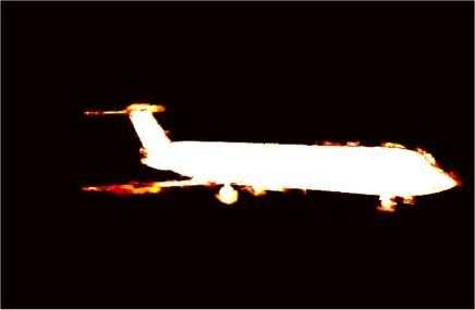
Figure 1: Comparing MAP inference and perturbation models. A segmentation is modeled by 𝐱=(x1,x2,,xn)𝐱subscript𝑥1subscript𝑥2subscript𝑥𝑛\mathbf{x}=(x_{1},x_{2},\ldots,x_{n}) where n𝑛n is the number of pixels and xi{0,1}subscript𝑥𝑖01x_{i}\in\{0,1\} is a discrete label relating a pixel to foreground (xi=1subscript𝑥𝑖1x_{i}=1) or background (xi=0subscript𝑥𝑖0x_{i}=0). θ(𝐱)𝜃𝐱\theta(\mathbf{x}) is the (super-modular) score of each segmentation. Left: original image along with the annotated boundary. Middle: the MAP segmentation argmax𝐱θ(𝐱)subscriptargmax𝐱𝜃𝐱\mathop{\mathrm{argmax}}_{\mathbf{x}}\theta(\mathbf{x}) recovered by the graph-cuts optimization algorithm using a region inside the boundary as seed pixels[15]. Note that the “optimal” solution is inaccurate because thin and long objects (wings) are labeled incorrectly. Right: The marginal probabilities of the perturb-max model estimated using 20 samples (random perturbations of θ(𝐱)𝜃𝐱\theta(\mathbf{x}) followed by executing graph-cuts). The information about the wings is recovered by these samples. Estimating the marginal probabilities of the corresponding Gibbs distribution by MCMC sampling is slow in practice and provably hard in theory [2, 9].

II Inference and random perturbations

We first describe the high dimensional statistical inference problems that motivate this work. These involve defining the potential function, the Gibbs distribution, and its entropy. Further background can be found in standard texts on graphical models [34]. We will then describe the MAP inference problem and describe how to use extreme value statistics to perform statistical inference while recovering the maximal assignment of randomly perturbed potential functions [35][36, pp.159–61]. To do this, we apply random perturbations to the potential function and use MAP solvers to produce a solution to the perturbed problem.

II-A High dimensional models, inference and extreme value statistics

Statistical inference for high dimensional problems involves reasoning about the states of discrete variables whose configurations (assignments of values) describe discrete structures. Suppose that our model has n𝑛n variables 𝐱=(x1,x2,,xn)𝐱subscript𝑥1subscript𝑥2subscript𝑥𝑛\mathbf{x}=(x_{1},x_{2},\ldots,x_{n}) where each xisubscript𝑥𝑖x_{i} takes values in a discrete set 𝒳isubscript𝒳𝑖\mathcal{X}_{i}. Let 𝒳=𝒳1×𝒳2××𝒳n𝒳subscript𝒳1subscript𝒳2subscript𝒳𝑛\mathcal{X}=\mathcal{X}_{1}\times\mathcal{X}_{2}\times\cdots\times\mathcal{X}_{n} so that 𝐱𝒳𝐱𝒳\mathbf{x}\in\mathcal{X}. Let Dom(θ)𝒳Dom𝜃𝒳\mathrm{Dom}(\theta)\subseteq\mathcal{X} be a subset of possible configurations and θ:𝒳:𝜃𝒳\theta:\mathcal{X}\to\mathbb{R} be a potential function that gives a score to an assignment or structure 𝐱𝐱\mathbf{x}. For convenience we define θ(𝐱)=𝜃𝐱\theta(\mathbf{x})=-\infty for 𝐱Dom(θ)𝐱Dom𝜃\mathbf{x}\notin\mathrm{Dom}(\theta). The potential function induces a probability distribution on configurations 𝐱=(x1,x2,,xn)𝐱subscript𝑥1subscript𝑥2subscript𝑥𝑛\mathbf{x}=(x_{1},x_{2},\ldots,x_{n}) via the Gibbs distribution:

p(𝐱)=Δ1Z(θ)exp(θ(𝐱))whereZ(θ)=Δ𝐱𝒳exp(θ(𝐱)).formulae-sequencesuperscriptΔ𝑝𝐱1𝑍𝜃𝜃𝐱wheresuperscriptΔ𝑍𝜃subscript𝐱𝒳𝜃𝐱\displaystyle p(\mathbf{x})\stackrel{{\scriptstyle\Delta}}{{=}}\frac{1}{Z(\theta)}\exp(\theta(\mathbf{x}))\qquad\mbox{where}\qquad Z(\theta)\stackrel{{\scriptstyle\Delta}}{{=}}\sum_{\mathbf{x}\in\mathcal{X}}\exp(\theta(\mathbf{x})). (1)

The normalization constant Z(θ)𝑍𝜃Z(\theta) is called the partition function. Sampling from the Gibbs distribution is often difficult because the partition function involves exponentially many terms (equal to the number of discrete structures in 𝒳𝒳\mathcal{X}). Computing the partition function is #P#𝑃\#P-hard in general (e.g., Valiant [37]).

II-B MAP inference

In practical inference tasks, the Gibbs distribution is constructed given observed data. Thus we call its maximizing assignment the maximum a-posteriori (MAP) prediction. We express the MAP inference problem as maximizing p(𝐱)𝑝𝐱p(\mathbf{x}), which is defined in Equation (1). Since the exponent is a monotone function, maximizing p(𝐱)𝑝𝐱p(\mathbf{x}) is equivalent to maximizing θ(𝐱)𝜃𝐱\theta(\mathbf{x}) and MAP prediction amounts to finding

𝐱=argmax𝐱𝒳θ(𝐱).superscript𝐱subscriptargmax𝐱𝒳𝜃𝐱\displaystyle{\mathbf{x}^{*}}=\mathop{\mathrm{argmax}}_{\mathbf{x}\in\mathcal{X}}\theta(\mathbf{x}). (2)

Methods for performing the optimization in (2) for high dimensional potential functions have been extensively researched in the last decade [15, 7, 17, 5, 18]. These have been useful in many cases of practical interest in computer vision, such as foreground-background image segmentation with supermodular potential functions (e.g., [38]), parsing and tagging (e.g., [6, 39]), branch and bound for scene understanding and pose estimation [40, 41], and dynamic programming predictions for outdoor scene understanding [42]. Although the run-time of these solvers can be exponential in the number of variables, they are often surprisingly effective in practice, [19, 43, 7, 44, 22].

II-C Inference and extreme value statistics

Although MAP prediction is NP-hard in general, it is often simpler than sampling from the Gibbs distribution. Nevertheless, usually there are several values of 𝐱𝐱\mathbf{x} whose scores θ(𝐱)𝜃𝐱\theta(\mathbf{x}) are close to θ(𝐱)𝜃superscript𝐱\theta({\mathbf{x}^{*}}) and we would like to sample these structures (see Figure 1). From such samples it is possible to estimate the amount of uncertainty in these models. A standard uncertainty measure is the entropy function:

H(p)𝐻𝑝\displaystyle H(p) =𝐱𝒳p(𝐱)logp(𝐱).absentsubscript𝐱𝒳𝑝𝐱𝑝𝐱\displaystyle=-\sum_{\mathbf{x}\in\mathcal{X}}p(\mathbf{x})\log p(\mathbf{x}). (3)

Sampling methods for posterior distributions often resort to MCMC algorithms that converge slowly in many practical settings [8, 9, 10].

An alternative approach to drawing unbiased samples from the Gibbs distribution is by randomly perturbing the potential function and solving the perturbed MAP problem. The “perturb-max” approach adds a random function γ:𝒳:𝛾𝒳\gamma:\mathcal{X}\to\mathbb{R} to the potential function in (1) and solves the resulting MAP problem:

𝐱=argmax𝐱𝒳{θ(𝐱)+γ(𝐱)},superscript𝐱subscriptargmax𝐱𝒳𝜃𝐱𝛾𝐱\displaystyle{\mathbf{x}^{*}}=\mathop{\mathrm{argmax}}_{\mathbf{x}\in\mathcal{X}}\left\{\theta(\mathbf{x})+\gamma(\mathbf{x})\right\}, (4)

where γ(𝐱)𝛾𝐱\gamma(\mathbf{x}) is a random function on 𝒳𝒳\mathcal{X}. The simplest approach to designing a perturbation function is to associate an independent and identically distributed (i.i.d.) random variable γ(𝐱)𝛾𝐱\gamma(\mathbf{x}) for each 𝐱𝒳𝐱𝒳\mathbf{x}\in\mathcal{X}. In this case, the distribution of the perturb-max value θ(𝐱)+γ(𝐱)𝜃𝐱𝛾𝐱\theta(\mathbf{x})+\gamma(\mathbf{x}) has an analytic form. To verify this observation we denote by F(t)=(γ(𝐱)t)𝐹𝑡𝛾𝐱𝑡F(t)=\mathbb{P}(\gamma(\mathbf{x})\leq t) the cumulative distribution function of γ(𝐱)𝛾𝐱\gamma(\mathbf{x}). The independence of γ(𝐱)𝛾𝐱\gamma(\mathbf{x}) across 𝐱𝒳𝐱𝒳\mathbf{x}\in\mathcal{X} implies that

γ(max𝐱𝒳{θ(𝐱)+γ(𝐱)}t)subscript𝛾subscript𝐱𝒳𝜃𝐱𝛾𝐱𝑡\displaystyle\mathbb{P}_{\gamma}\left(\max_{\mathbf{x}\in\mathcal{X}}\left\{\theta(\mathbf{x})+\gamma(\mathbf{x})\right\}\leq t\right) =γ(𝐱𝒳:{θ(𝐱)+γ(𝐱)}t)\displaystyle=\mathbb{P}_{\gamma}\left(\forall\mathbf{x}\in\mathcal{X}:\left\{\theta(\mathbf{x})+\gamma(\mathbf{x})\right\}\leq t\right) (5)
=γ(𝐱𝒳:{θ(𝐱)+γ(𝐱)}t)\displaystyle=\mathbb{P}_{\gamma}\left(\forall\mathbf{x}\in\mathcal{X}:\left\{\theta(\mathbf{x})+\gamma(\mathbf{x})\right\}\leq t\right) (6)
=𝐱𝒳F(tθ(𝐱)).absentsubscriptproduct𝐱𝒳𝐹𝑡𝜃𝐱\displaystyle=\prod_{\mathbf{x}\in\mathcal{X}}F(t-\theta(\mathbf{x})). (7)

Unfortunately, the product of cumulative distribution functions is not usually a simple distribution.

The Gumbel, Fréchet, and Weibull distributions, used in extremal statistics, are max-stable distributions: the product 𝐱𝒳F(tθ(𝐱))subscriptproduct𝐱𝒳𝐹𝑡𝜃𝐱\prod_{\mathbf{x}\in\mathcal{X}}F(t-\theta(\mathbf{x})) can be described by their own cumulative distribution function F()𝐹F(\cdot) [45, 46, 47]. In this work we focus on the Gumbel distribution with zero mean, which is described by a doubly exponential cumulative distribution function

G(t)=exp(exp((t+c))),𝐺𝑡𝑡𝑐\displaystyle G(t)=\exp(-\exp(-(t+c))), (8)

where c0.5772𝑐0.5772c\approx 0.5772 is the Euler-Mascheroni constant. Throughout our work we use the max-stability of the Gumbel distribution as described in the following theorem.

Theorem 1 (Max-stability of Gumbel perturbations [45, 46, 47])

Let γ={γ(𝐱):𝐱𝒳}𝛾conditional-set𝛾𝐱𝐱𝒳\gamma=\{\gamma(\mathbf{x}):\mathbf{x}\in\mathcal{X}\} be a collection of i.i.d. Gumbel random variables whose cumulative distribution function is given by G(t)=(γ(𝐱)t)=exp(exp((t+c)))𝐺𝑡𝛾𝐱𝑡𝑡𝑐G(t)=\mathbb{P}(\gamma(\mathbf{x})\leq t)=\exp(-\exp(-(t+c))). Then the random variable max𝐱𝒳{θ(𝐱)+γ(𝐱)}subscript𝐱𝒳𝜃𝐱𝛾𝐱\max_{\mathbf{x}\in\mathcal{X}}\left\{\theta(\mathbf{x})+\gamma(\mathbf{x})\right\} is distributed according to the Gumbel distribution whose mean is the log-partition function logZ(θ)𝑍𝜃\log Z(\theta).

Proof:

The proof is known, but we include it for completeness. By the independence assumption,

γ(max𝐱𝒳{θ(𝐱)+γ(𝐱)}t)=xXγ(𝐱)(θ(𝐱)+γ(𝐱)t).subscript𝛾subscript𝐱𝒳𝜃𝐱𝛾𝐱𝑡subscriptproduct𝑥𝑋subscript𝛾𝐱𝜃𝐱𝛾𝐱𝑡\displaystyle\mathbb{P}_{\gamma}\left(\max_{\mathbf{x}\in\mathcal{X}}\{\theta(\mathbf{x})+\gamma(\mathbf{x})\}\leq t\right)=\prod_{x\in X}\mathbb{P}_{\gamma(\mathbf{x})}\left(\theta(\mathbf{x})+\gamma(\mathbf{x})\leq t\right).

The random variable θ(𝐱)+γ(𝐱)𝜃𝐱𝛾𝐱\theta(\mathbf{x})+\gamma(\mathbf{x}) follows the Gumbel distribution with mean θ(𝐱)𝜃𝐱\theta(\mathbf{x}). Therefore

γ(x)(θ(𝐱)+γ(𝐱)t)=G(tθ(𝐱)).subscript𝛾𝑥𝜃𝐱𝛾𝐱𝑡𝐺𝑡𝜃𝐱\displaystyle\mathbb{P}_{\gamma(x)}\left(\theta(\mathbf{x})+\gamma(\mathbf{x})\leq t\right)=G(t-\theta(\mathbf{x})).

Lastly, the double exponential form of the Gumbel distribution yields the result:

xXG(tθ(𝐱))subscriptproduct𝑥𝑋𝐺𝑡𝜃𝐱\displaystyle\prod_{x\in X}G(t-\theta(\mathbf{x})) =exp(𝐱𝒳exp((tθ(𝐱)+c)))absentsubscript𝐱𝒳𝑡𝜃𝐱𝑐\displaystyle=\exp\left(-\sum_{\mathbf{x}\in\mathcal{X}}\exp\left(-(t-\theta(\mathbf{x})+c)\right)\right)
=exp(exp((t+clogZ(θ)))\displaystyle=\exp\left(-\exp(-(t+c-\log Z(\theta))\right)
=G(tlogZ(θ)).absent𝐺𝑡𝑍𝜃\displaystyle=G(t-\log Z(\theta)).

We can use the log-partition function to recover the moments of the Gibbs distribution. Thus the log-partition function characterizes the stability of the randomized MAP predictor 𝐱superscript𝐱{\mathbf{x}^{*}} in (4).

Corollary 1 (Sampling from perturb-max models [48, 49, 50])

Under the conditions of Theorem 1 the Gibbs distribution measures the stability of the perturb-max argument. That is, for all 𝐱^^𝐱\hat{\mathbf{x}},

exp(θ(𝐱^))Z(θ)𝜃^𝐱𝑍𝜃\displaystyle\frac{\exp(\theta(\hat{\mathbf{x}}))}{Z(\theta)} =γ(𝐱^=argmax𝐱𝒳{θ(𝐱)+γ(𝐱)}),absentsubscript𝛾^𝐱subscriptargmax𝐱𝒳𝜃𝐱𝛾𝐱\displaystyle=\mathbb{P}_{\gamma}\left(\hat{\mathbf{x}}=\mathop{\mathrm{argmax}}_{\mathbf{x}\in\mathcal{X}}\left\{\theta(\mathbf{x})+\gamma(\mathbf{x})\right\}\right), (9)
Proof:

From Theorem 1, we have logZ(θ)=𝔼γ[max𝐱𝒳{θ(𝐱)+γ(𝐱)}]𝑍𝜃subscript𝔼𝛾delimited-[]subscript𝐱𝒳𝜃𝐱𝛾𝐱\log Z(\theta)=\mathbb{E}_{\gamma}[\max_{\mathbf{x}\in\mathcal{X}}\left\{\theta(\mathbf{x})+\gamma(\mathbf{x})\right\}], so we can take the derivative with respect to some θ(𝐱^)𝜃^𝐱\theta(\hat{\mathbf{x}}). We note that by differentiating the left hand side we get the Gibbs distribution:

logZ(θ)θ(𝐱^)=exp(θ(𝐱^))Z(θ).𝑍𝜃𝜃^𝐱𝜃^𝐱𝑍𝜃\displaystyle\frac{\partial\log Z(\theta)}{\partial\theta(\hat{\mathbf{x}})}=\frac{\exp(\theta(\hat{\mathbf{x}}))}{Z(\theta)}.

Differentiating the right hand side is slightly more involved. First, we can differentiate under the integral sign (cf. [51]) so

θ(𝐱^)|𝒳|max𝐱𝒳{θ(𝐱)+γ(𝐱)}𝑑γ𝜃^𝐱subscriptsuperscript𝒳subscript𝐱𝒳𝜃𝐱𝛾𝐱differential-d𝛾\displaystyle\frac{\partial}{\partial\theta(\hat{\mathbf{x}})}\int_{\mathbb{R}^{|\mathcal{X}|}}\max_{\mathbf{x}\in\mathcal{X}}\left\{\theta(\mathbf{x})+\gamma(\mathbf{x})\right\}d\gamma =|𝒳|θ(𝐱^)max𝐱𝒳{θ(𝐱)+γ(𝐱)}𝑑γ.absentsubscriptsuperscript𝒳𝜃^𝐱subscript𝐱𝒳𝜃𝐱𝛾𝐱differential-d𝛾\displaystyle=\int_{\mathbb{R}^{|\mathcal{X}|}}\frac{\partial}{\partial\theta(\hat{\mathbf{x}})}\max_{\mathbf{x}\in\mathcal{X}}\left\{\theta(\mathbf{x})+\gamma(\mathbf{x})\right\}d\gamma.

The (sub)gradient of the max-function is the indicator function (an application of Danskin’s Theorem [52]):

θ(𝐱^)max𝐱𝒳{θ(𝐱)+γ(𝐱)}𝜃^𝐱subscript𝐱𝒳𝜃𝐱𝛾𝐱\displaystyle\frac{\partial}{\partial\theta(\hat{\mathbf{x}})}\max_{\mathbf{x}\in\mathcal{X}}\left\{\theta(\mathbf{x})+\gamma(\mathbf{x})\right\} =𝟏(𝐱^=argmax𝐱𝒳{θ(𝐱)+γ(𝐱)}).absent1^𝐱subscriptargmax𝐱𝒳𝜃𝐱𝛾𝐱\displaystyle=\mathbf{1}\left(\hat{\mathbf{x}}=\mathop{\mathrm{argmax}}_{\mathbf{x}\in\mathcal{X}}\left\{\theta(\mathbf{x})+\gamma(\mathbf{x})\right\}\right).

The corollary then follows by applying the expectation to both sides of the last equation. ∎

An alternative proof of the preceding corollary can be given by considering the probability density function g(t)=G(t)𝑔𝑡superscript𝐺𝑡g(t)=G^{\prime}(t) of the Gumbel distribution. This proof consists of two steps. First, the probability that 𝐱^^𝐱\hat{\mathbf{x}} maximizes θ(𝐱)+γ(𝐱)𝜃𝐱𝛾𝐱\theta(\mathbf{x})+\gamma(\mathbf{x}) is g(tθ(𝐱^))𝐱𝐱^G(tθ(𝐱))dt𝑔𝑡𝜃^𝐱subscriptproduct𝐱^𝐱𝐺𝑡𝜃𝐱𝑑𝑡\int g(t-\theta(\hat{\mathbf{x}}))\prod_{\mathbf{x}\neq\hat{\mathbf{x}}}G(t-\theta(\mathbf{x}))dt. Second, g(tθ(𝐱^))=exp(θ(𝐱^))exp((t+c))G(tθ(𝐱^))𝑔𝑡𝜃^𝐱𝜃^𝐱𝑡𝑐𝐺𝑡𝜃^𝐱g(t-\theta(\hat{\mathbf{x}}))=\exp(\theta(\hat{\mathbf{x}}))\cdot\exp(-(t+c))G(t-\theta(\hat{\mathbf{x}})). Thus, the probability that 𝐱^^𝐱\hat{\mathbf{x}} maximizes θ(𝐱)+γ(𝐱)𝜃𝐱𝛾𝐱\theta(\mathbf{x})+\gamma(\mathbf{x}) is proportional to exp(θ(𝐱^))𝜃^𝐱\exp(\theta(\hat{\mathbf{x}})), i.e., it is the Gibbs distribution.

We can also use the random MAP perturbation to estimate the entropy of the Gibbs distribution.

Corollary 2

Let p(x)𝑝𝑥p(x) be the Gibbs distribution, defined in (3) and let 𝐱superscript𝐱{\mathbf{x}^{*}} be given by (4). Under the conditions of Theorem 1,

H(p)𝐻𝑝\displaystyle H(p) =𝔼γ[γ(𝐱)].absentsubscript𝔼𝛾delimited-[]𝛾superscript𝐱\displaystyle=\mathbb{E}_{\gamma}\left[\gamma({\mathbf{x}^{*}})\right].
Proof:

The proof consists of evaluating the entropy in Equation (3) and using Theorem 1 to replace logZ(θ)𝑍𝜃\log Z(\theta) with 𝔼γ[θ(𝐱)+γ(𝐱)]subscript𝔼𝛾delimited-[]𝜃superscript𝐱𝛾superscript𝐱\mathbb{E}_{\gamma}[\theta({\mathbf{x}^{*}})+\gamma({\mathbf{x}^{*}})]. Formally,

H(p)𝐻𝑝\displaystyle H(p) =𝐱𝒳p(𝐱)θ(𝐱)+𝔼γ[θ(𝐱)+γ(𝐱)]absentsubscript𝐱𝒳𝑝𝐱𝜃𝐱subscript𝔼𝛾delimited-[]𝜃superscript𝐱𝛾superscript𝐱\displaystyle=-\sum_{\mathbf{x}\in\mathcal{X}}p(\mathbf{x})\theta(\mathbf{x})+\mathbb{E}_{\gamma}[\theta({\mathbf{x}^{*}})+\gamma({\mathbf{x}^{*}})]
=𝐱𝒳p(𝐱)θ(𝐱)+𝐱𝒳θ(𝐱)γ(𝐱=𝐱)+𝔼γ[γ(𝐱)]absentsubscript𝐱𝒳𝑝𝐱𝜃𝐱subscript𝐱𝒳𝜃𝐱subscript𝛾superscript𝐱𝐱subscript𝔼𝛾delimited-[]𝛾superscript𝐱\displaystyle=-\sum_{\mathbf{x}\in\mathcal{X}}p(\mathbf{x})\theta(\mathbf{x})+\sum_{\mathbf{x}\in\mathcal{X}}\theta(\mathbf{x})\mathbb{P}_{\gamma}({\mathbf{x}^{*}}=\mathbf{x})+\mathbb{E}_{\gamma}[\gamma({\mathbf{x}^{*}})]
=𝔼γ[γ(𝐱)],absentsubscript𝔼𝛾delimited-[]𝛾superscript𝐱\displaystyle=\mathbb{E}_{\gamma}[\gamma({\mathbf{x}^{*}})],

where in the last line we used Corollary 1, which says γ(𝐱=𝐱)=p(𝐱)subscript𝛾superscript𝐱𝐱𝑝𝐱\mathbb{P}_{\gamma}({\mathbf{x}^{*}}=\mathbf{x})=p(\mathbf{x}). ∎

A direct proof of the preceding corollary can be given by showing that 𝔼γ[γ(𝐱)1[𝐱^=𝐱]]=p(𝐱^)logp(𝐱^)subscript𝔼𝛾delimited-[]𝛾superscript𝐱1delimited-[]^𝐱superscript𝐱𝑝^𝐱𝑝^𝐱\mathbb{E}_{\gamma}\left[\gamma({\mathbf{x}^{*}})\cdot 1[\hat{\mathbf{x}}={\mathbf{x}^{*}}]\right]=-p(\hat{\mathbf{x}})\log p(\hat{\mathbf{x}}) while the entropy is then attained by summing over all 𝐱^^𝐱\hat{\mathbf{x}}, since 𝐱^𝒳1[𝐱^=𝐱]=1subscript^𝐱𝒳1delimited-[]^𝐱superscript𝐱1\sum_{\hat{\mathbf{x}}\in\mathcal{X}}1[\hat{\mathbf{x}}={\mathbf{x}^{*}}]=1. To establish this equality we note that

𝔼γ[γ(𝐱)1[𝐱^=𝐱]]subscript𝔼𝛾delimited-[]𝛾superscript𝐱1delimited-[]^𝐱superscript𝐱\displaystyle\mathbb{E}_{\gamma}\left[\gamma({\mathbf{x}^{*}})\cdot 1[\hat{\mathbf{x}}={\mathbf{x}^{*}}]\right] =(tθ(𝐱^))g(tθ(𝐱^))𝐱𝐱^G(tθ(𝐱))dt.absent𝑡𝜃^𝐱𝑔𝑡𝜃^𝐱subscriptproduct𝐱^𝐱𝐺𝑡𝜃𝐱𝑑𝑡\displaystyle=\int(t-\theta(\hat{\mathbf{x}}))g(t-\theta(\hat{\mathbf{x}}))\prod_{\mathbf{x}\neq\hat{\mathbf{x}}}G(t-\theta(\mathbf{x}))dt.

Using the relation between g(t)𝑔𝑡g(t) and G(t)𝐺𝑡G(t) and the fact that xXG(tθ(x))=G(tlogZ(θ))subscriptproduct𝑥𝑋𝐺𝑡𝜃𝑥𝐺𝑡𝑍𝜃\prod_{x\in X}G(t-\theta(x))=G(t-\log Z(\theta)) while changing the integration variable to t^=tθ(𝐱^)^𝑡𝑡𝜃^𝐱\hat{t}=t-\theta(\hat{\mathbf{x}}) we can rephrase this quantity as texp((c+t))G(t+logp(𝐱^))𝑑t𝑡𝑐𝑡𝐺𝑡𝑝^𝐱differential-d𝑡\int t\exp(-(c+t))G(t+\log p(\hat{\mathbf{x}}))dt. Again by using the relation between g(t+logp(𝐱^))𝑔𝑡𝑝^𝐱g(t+\log p(\hat{\mathbf{x}})) and G(t+logp(𝐱^))𝐺𝑡𝑝^𝐱G(t+\log p(\hat{\mathbf{x}})) we derive that 𝔼γ[γ(𝐱)1[𝐱^=𝐱]]=p(𝐱^)tg(t+logp(𝐱^))𝑑tsubscript𝔼𝛾delimited-[]𝛾superscript𝐱1delimited-[]^𝐱superscript𝐱𝑝^𝐱𝑡𝑔𝑡𝑝^𝐱differential-d𝑡\mathbb{E}_{\gamma}\left[\gamma({\mathbf{x}^{*}})\cdot 1[\hat{\mathbf{x}}={\mathbf{x}^{*}}]\right]=p(\hat{\mathbf{x}})\int tg(t+\log p(\hat{\mathbf{x}}))dt while the integral is now the mean of a Gumbel random variable with expected value of logp(𝐱^)𝑝^𝐱-\log p(\hat{\mathbf{x}}).

The preceding derivations show that perturbing the potential function θ(𝐱)𝜃𝐱\theta(\mathbf{x}) and then finding the MAP estimate 𝐱superscript𝐱{\mathbf{x}^{*}} of the perturbed Gibbs distribution allows us to perform many core tasks for high-dimensional statistical inference by using i.i.d. Gumbel perturbations. The distribution of 𝐱superscript𝐱{\mathbf{x}^{*}} is p(𝐱)𝑝𝐱p(\mathbf{x}), its expected maximum value is the log-partition function, and the expected maximizing perturbation is the entropy of p(𝐱)𝑝𝐱p(\mathbf{x}). While theoretically appealing, these derivations are computationally intractable when dealing with high-dimensional structures. These derivations involve generating high-dimensional perturbations, namely |𝒳|𝒳|\mathcal{X}| random variables in the image of γ()𝛾\gamma(\cdot), one for each assignment in 𝒳=𝒳1×𝒳n𝒳subscript𝒳1subscript𝒳𝑛\mathcal{X}=\mathcal{X}_{1}\times\cdots\mathcal{X}_{n}, which grows exponentially with n𝑛n. The goal of this paper is to apply high-dimensional inference using max-solvers that involve a low-dimensional perturbation term. More specifically, we wish to involve only a linear (in n𝑛n) number of random variables.

III Low-dimensional perturbations

We now turn towards making the perturb-max framework more practical. The log-partition function logZ(θ)𝑍𝜃\log Z(\theta) (c.f. Theorem 2) is the key quantity to understand: its gradient is the Gibbs distribution and the entropy is its Fenchel dual. It is well-known that computing Z(θ)𝑍𝜃Z(\theta) for high-dimensional models is challenging because of the exponential size of 𝒳𝒳\mathcal{X}. This complexity carries over to the perturb-max approach to estimating the log-partition function, which also involves generating an exponential number of Gumbel random variables. In this section we show that the log-partition function can be computed using low-dimensional perturbations in a sequence of expected max-value computations. This will give us some insight on performing high dimensional inference using low dimensional perturbations. In what follows we will use the notation 𝐱ijsuperscriptsubscript𝐱𝑖𝑗\mathbf{x}_{i}^{j} to refer to the tuple (xi,xi+1,,xj)subscript𝑥𝑖subscript𝑥𝑖1subscript𝑥𝑗(x_{i},x_{i+1},\ldots,x_{j}) for i<j𝑖𝑗i<j, with 𝐱=𝐱1n𝐱superscriptsubscript𝐱1𝑛\mathbf{x}=\mathbf{x}_{1}^{n}.

The partition function has a self-reducible form. That is, we can compute it iteratively while computing partial partition functions of lower dimensions:

Z(θ)=x1x2xnexp(θ(x1,x2,,xn)).𝑍𝜃subscriptsubscript𝑥1subscriptsubscript𝑥2subscriptsubscript𝑥𝑛𝜃subscript𝑥1subscript𝑥2subscript𝑥𝑛\displaystyle Z(\theta)=\sum_{x_{1}}\sum_{x_{2}}\cdots\sum_{x_{n}}\exp(\theta(x_{1},x_{2},\ldots,x_{n})). (10)

For example, the partition function is the sum, over x1subscript𝑥1x_{1}, of partial partition functions x2,,xnexp(θ(𝐱))subscriptsubscript𝑥2subscript𝑥𝑛𝜃𝐱\sum_{x_{2},\ldots,x_{n}}\exp(\theta(\mathbf{x})). Fixing x1,x2,,xisubscript𝑥1subscript𝑥2subscript𝑥𝑖x_{1},x_{2},\ldots,x_{i}, the remaining summations are partial partition functions xi+1,,xnexp(θ(𝐱))subscriptsubscript𝑥𝑖1subscript𝑥𝑛𝜃𝐱\sum_{x_{i+1},\ldots,x_{n}}\exp(\theta(\mathbf{x})). With this in mind, we can compute each partial partition function using Theorem 1 but with low-dimensional perturbations for each partial partition.

Theorem 2

Let {γi(xi)}xi𝒳i,i=1,,nsubscriptsubscript𝛾𝑖subscript𝑥𝑖formulae-sequencesubscript𝑥𝑖subscript𝒳𝑖𝑖1𝑛\{\gamma_{i}(x_{i})\}_{x_{i}\in\mathcal{X}_{i},i=1,\ldots,n}, be a collection of independent and identically distributed (i.i.d.) random variables following the Gumbel distribution, defined in Theorem 1. Define γi={γi(xi)}xi𝒳isubscript𝛾𝑖subscriptsubscript𝛾𝑖subscript𝑥𝑖subscript𝑥𝑖subscript𝒳𝑖\gamma_{i}=\{\gamma_{i}(x_{i})\}_{x_{i}\in\mathcal{X}_{i}}. Then

logZ=𝔼γ1maxx1𝔼γnmaxxn{θ(𝐱)+i=1nγi(xi)}.𝑍subscript𝔼subscript𝛾1subscriptsubscript𝑥1subscript𝔼subscript𝛾𝑛subscriptsubscript𝑥𝑛𝜃𝐱superscriptsubscript𝑖1𝑛subscript𝛾𝑖subscript𝑥𝑖\displaystyle\log Z=\mathbb{E}_{\gamma_{1}}\max_{x_{1}}\cdots\mathbb{E}_{\gamma_{n}}\max_{x_{n}}\left\{\theta(\mathbf{x})+\sum_{i=1}^{n}\gamma_{i}(x_{i})\right\}. (11)
Proof:

The result follows from applying Theorem 1 iteratively. Let θn(𝐱1n)=θ(𝐱1n)subscript𝜃𝑛superscriptsubscript𝐱1𝑛𝜃superscriptsubscript𝐱1𝑛\theta_{n}(\mathbf{x}_{1}^{n})=\theta(\mathbf{x}_{1}^{n}) and define

θi1(𝐱1i1)=𝔼γimaxxi{θi(𝐱1i)+γi(xi)}i=2,3,,nformulae-sequencesubscript𝜃𝑖1superscriptsubscript𝐱1𝑖1subscript𝔼subscript𝛾𝑖subscriptsubscript𝑥𝑖subscript𝜃𝑖superscriptsubscript𝐱1𝑖subscript𝛾𝑖subscript𝑥𝑖𝑖23𝑛\displaystyle\theta_{i-1}(\mathbf{x}_{1}^{i-1})=\mathbb{E}_{\gamma_{i}}\max_{x_{i}}\{\theta_{i}(\mathbf{x}_{1}^{i})+\gamma_{i}(x_{i})\}\qquad i=2,3,\ldots,n

If we think of 𝐱1i1superscriptsubscript𝐱1𝑖1\mathbf{x}_{1}^{i-1} as fixed and apply Theorem 1 to θi(𝐱1i1,xi)subscript𝜃𝑖superscriptsubscript𝐱1𝑖1subscript𝑥𝑖\theta_{i}(\mathbf{x}_{1}^{i-1},x_{i}), we see that from (10),

θi1(𝐱1i1)=logxiexp(θi(𝐱1i)).subscript𝜃𝑖1superscriptsubscript𝐱1𝑖1subscriptsubscript𝑥𝑖subscript𝜃𝑖superscriptsubscript𝐱1𝑖\displaystyle\theta_{i-1}(\mathbf{x}_{1}^{i-1})=\log\sum_{x_{i}}\exp(\theta_{i}(\mathbf{x}_{1}^{i})).

Applying this for i=n𝑖𝑛i=n to i=2𝑖2i=2, we obtain (11). ∎

The computational complexity of the alternating procedure in (11) is still exponential in n𝑛n. For example, the innermost iteration θn1(𝐱1n1)=𝔼γnmaxxn{θn(𝐱1n)+γn(xn)}subscript𝜃𝑛1superscriptsubscript𝐱1𝑛1subscript𝔼subscript𝛾𝑛subscriptsubscript𝑥𝑛subscript𝜃𝑛superscriptsubscript𝐱1𝑛subscript𝛾𝑛subscript𝑥𝑛\theta_{n-1}(\mathbf{x}_{1}^{n-1})=\mathbb{E}_{\gamma_{n}}\max_{x_{n}}\{\theta_{n}(\mathbf{x}_{1}^{n})+\gamma_{n}(x_{n})\} needs to be estimated for every 𝐱1n1=(x1,x2,,xn1)superscriptsubscript𝐱1𝑛1subscript𝑥1subscript𝑥2subscript𝑥𝑛1\mathbf{x}_{1}^{n-1}=(x_{1},x_{2},\ldots,x_{n-1}), which is growing exponentially with n𝑛n. Thus from computational perspective the alternating formulation in Theorem 2 is just as inefficient as the formulation in Theorem 1. Nevertheless, this is the building block that enables inference in high-dimensional problems using low dimensional perturbations and max-solvers. Specifically, it provides the means for a new sampling algorithm from the Gibbs distribution and bounds on the log-partition and entropy functions.

III-A Ideal Sampling

Sampling from the Gibbs distribution is inherently tied to estimating the partition function. If we could compute the partition function exactly, then we could sample from the Gibbs distribution sequentially: for dimension i=1,2,,n𝑖12𝑛i=1,2,\ldots,n sample xisubscript𝑥𝑖x_{i} with probability which is proportional to 𝐱i+1nexp(θ(𝐱))subscriptsuperscriptsubscript𝐱𝑖1𝑛𝜃𝐱\sum_{\mathbf{x}_{i+1}^{n}}\exp(\theta(\mathbf{x})). Unfortunately, directly computing the partition function is #P-hard. Instead, we construct a family of self-reducible upper bounds which imitate the partition function behavior, namely by bounding the summation over its exponentiations.

Corollary 3

Let {γi(xi)}xi𝒳i,i=1,2,,nsubscriptsubscript𝛾𝑖subscript𝑥𝑖formulae-sequencesubscript𝑥𝑖subscript𝒳𝑖𝑖12𝑛\{\gamma_{i}(x_{i})\}_{x_{i}\in\mathcal{X}_{i},i=1,2,\ldots,n} be a collection of i.i.d. random variables, each following the Gumbel distribution with zero mean. Set

ϕj(𝐱1j)=𝔼γ[maxxj+1n{θ(𝐱)+i=j+1nγi(xi)}].subscriptitalic-ϕ𝑗superscriptsubscript𝐱1𝑗subscript𝔼𝛾delimited-[]subscriptsuperscriptsubscript𝑥𝑗1𝑛𝜃𝐱superscriptsubscript𝑖𝑗1𝑛subscript𝛾𝑖subscript𝑥𝑖\displaystyle\phi_{j}(\mathbf{x}_{1}^{j})=\mathbb{E}_{\gamma}\left[\max_{x_{j+1}^{n}}\{\theta(\mathbf{x})+\sum_{i=j+1}^{n}\gamma_{i}(x_{i})\}\right]. (12)

Then for every j=1,,n1𝑗1𝑛1j=1,\ldots,n-1 and every 𝐱=𝐱1n𝐱superscriptsubscript𝐱1𝑛\mathbf{x}=\mathbf{x}_{1}^{n} the following inequality holds:

xjexp(ϕj(𝐱1j))exp(ϕj1(𝐱1j1)).subscriptsubscript𝑥𝑗subscriptitalic-ϕ𝑗superscriptsubscript𝐱1𝑗subscriptitalic-ϕ𝑗1superscriptsubscript𝐱1𝑗1\displaystyle\sum_{x_{j}}\exp\left(\phi_{j}(\mathbf{x}_{1}^{j})\right)\leq\exp\left(\phi_{j-1}(\mathbf{x}_{1}^{j-1})\right). (13)

In particular, for j=n𝑗𝑛j=n we have xnexp(θ(𝐱1n))=exp(ϕn1(𝐱1n1))subscriptsubscript𝑥𝑛𝜃superscriptsubscript𝐱1𝑛subscriptitalic-ϕ𝑛1superscriptsubscript𝐱1𝑛1\sum_{x_{n}}\exp(\theta(\mathbf{x}_{1}^{n}))=\exp\left(\phi_{n-1}(\mathbf{x}_{1}^{n-1})\right).

Proof:

The result is an application of the perturb-max interpretation of the partition function in Theorem 1. Intuitively, these bounds correspond to moving expectations outside the maximization operations in Theorem 2, each move resulting in a different bound. Formally, the left hand side can be expanded as

𝔼γj[maxxj𝔼γj+1,,γn[max𝐱j+1n{θ(𝐱1n)+i=jnγi(xi)}]],subscript𝔼subscript𝛾𝑗delimited-[]subscriptsubscript𝑥𝑗subscript𝔼subscript𝛾𝑗1subscript𝛾𝑛delimited-[]subscriptsuperscriptsubscript𝐱𝑗1𝑛𝜃superscriptsubscript𝐱1𝑛superscriptsubscript𝑖𝑗𝑛subscript𝛾𝑖subscript𝑥𝑖\displaystyle\mathbb{E}_{\gamma_{j}}\left[\max_{x_{j}}\mathbb{E}_{\gamma_{j+1},\ldots,\gamma_{n}}\left[\max_{\mathbf{x}_{j+1}^{n}}\left\{\theta(\mathbf{x}_{1}^{n})+\sum_{i=j}^{n}\gamma_{i}(x_{i})\right\}\right]\right], (14)

while the right hand side is attained by alternating the maximization with respect to xjsubscript𝑥𝑗x_{j} with the expectation of γj+1,,γnsubscript𝛾𝑗1subscript𝛾𝑛\gamma_{j+1},\ldots,\gamma_{n}. The proof then follows by exponentiating both sides.∎

The above corollary is similar in nature to variational approaches that have been extensively developed to efficiently estimate the partition function in large-scale problems. These are often inner-bound methods where a simpler distribution is optimized as an approximation to the posterior in a KL-divergence sense (e.g., mean field) [53]. Variational upper bounds on the other hand are convex, usually derived by replacing the entropy term with a simpler surrogate function and relaxing constraints on sufficient statistics (see, e.g., [54]).

We use these upper bounds for every dimension i=1,,n𝑖1𝑛i=1,\ldots,n to sample from a probability distribution that follows a summation over exponential functions, with a discrepancy that is described by the upper bound. This is formalized below in Algorithm 1. Note that 𝐱=(𝐱1j1,xj,𝐱j+1n)𝐱superscriptsubscript𝐱1𝑗1subscript𝑥𝑗superscriptsubscript𝐱𝑗1𝑛\mathbf{x}=(\mathbf{x}_{1}^{j-1},x_{j},\mathbf{x}_{j+1}^{n}).

Algorithm 1 Unbiased sampling from Gibbs distribution
Potential function θ(𝐱)𝜃𝐱\theta(\mathbf{x}), MAP solver
Initial step j=1𝑗1j=1.
while j<n𝑗𝑛j<n do
     For all x𝒳j𝑥subscript𝒳𝑗x\in\mathcal{X}_{j} compute
ϕj(𝐱1j1,x)=𝔼γ[max𝐱j+1n{θ(𝐱1j1,x,𝐱j+1n)+i=j+1nγi(xi)}].subscriptitalic-ϕ𝑗superscriptsubscript𝐱1𝑗1𝑥subscript𝔼𝛾delimited-[]subscriptsuperscriptsubscript𝐱𝑗1𝑛𝜃superscriptsubscript𝐱1𝑗1𝑥superscriptsubscript𝐱𝑗1𝑛superscriptsubscript𝑖𝑗1𝑛subscript𝛾𝑖subscript𝑥𝑖\displaystyle\phi_{j}(\mathbf{x}_{1}^{j-1},x)=\mathbb{E}_{\gamma}\left[\max_{\mathbf{x}_{j+1}^{n}}\left\{\theta(\mathbf{x}_{1}^{j-1},x,\mathbf{x}_{j+1}^{n})+\sum_{i=j+1}^{n}\gamma_{i}(x_{i})\right\}\right]. (15)
     Define a distribution on 𝒳j{r}subscript𝒳𝑗𝑟\mathcal{X}_{j}\cup\{r\}:
pj(x)subscript𝑝𝑗𝑥\displaystyle p_{j}(x) =exp(ϕj(𝐱1j1,x))exp(ϕj1(𝐱1j1)),x𝒳jformulae-sequenceabsentsubscriptitalic-ϕ𝑗superscriptsubscript𝐱1𝑗1𝑥subscriptitalic-ϕ𝑗1superscriptsubscript𝐱1𝑗1𝑥subscript𝒳𝑗\displaystyle=\frac{\exp\left(\phi_{j}(\mathbf{x}_{1}^{j-1},x)\right)}{\exp\left(\phi_{j-1}(\mathbf{x}_{1}^{j-1})\right)},\qquad x\in\mathcal{X}_{j} (16)
pj(r)subscript𝑝𝑗𝑟\displaystyle p_{j}(r) =1x𝒳jpj(x)absent1subscript𝑥subscript𝒳𝑗subscript𝑝𝑗𝑥\displaystyle=1-\sum_{x\in\mathcal{X}_{j}}p_{j}(x) (17)
     Sample xjsubscript𝑥𝑗x_{j} from pj()subscript𝑝𝑗p_{j}(\cdot).
     if xj=rsubscript𝑥𝑗𝑟x_{j}=r then
         Set j=1𝑗1j=1 to restart sampler.
     else xj𝒳jsubscript𝑥𝑗subscript𝒳𝑗x_{j}\in\mathcal{X}_{j}
         Set jj+1𝑗𝑗1j\leftarrow j+1.
     end if
end while
return 𝐱=(x1,x2,,xn)𝐱subscript𝑥1subscript𝑥2subscript𝑥𝑛\mathbf{x}=(x_{1},x_{2},\ldots,x_{n})

This algorithm is forced to restart the entire sample if it samples the “reject” symbol r𝑟r at any iteration. We say the algorithm accepts if it terminates with an output 𝐱𝐱\mathbf{x}. The probability of accepting with particular 𝐱𝐱\mathbf{x} is the product of the probabilities of sampling xjsubscript𝑥𝑗x_{j} in round j𝑗j for j[n]𝑗delimited-[]𝑛j\in[n]. Since these upper bounds are self-reducible, i.e., for every dimension i𝑖i we are using the same quantities that were computed in the previous dimensions 1,2,,i112𝑖11,2,\ldots,i-1, we are sampling an accepted configuration proportionally to exp(θ(𝐱))𝜃𝐱\exp(\theta(\mathbf{x})), the full Gibbs distribution. This is summarized in the following theorem.

Theorem 3

Let p(𝐱)𝑝𝐱p(\mathbf{x}) be the Gibbs distribution defined in (1) and let {γi(xi)}subscript𝛾𝑖subscript𝑥𝑖\{\gamma_{i}(x_{i})\} be a collection of i.i.d. random variables following the Gumbel distribution with zero mean given in (8). Then

(Algorithm 1 accepts)=Z(θ)/exp(𝔼γ[max𝐱{θ(𝐱)+i=1nγi(xi)}]).Algorithm 1 accepts𝑍𝜃subscript𝔼𝛾delimited-[]subscript𝐱𝜃𝐱superscriptsubscript𝑖1𝑛subscript𝛾𝑖subscript𝑥𝑖\displaystyle\mathbb{P}\left(\textrm{Algorithm \ref{alg:unbiased} accepts}\right)=Z(\theta)\big{/}\exp\left(\mathbb{E}_{\gamma}\left[\max_{\mathbf{x}}\{\theta(\mathbf{x})+\sum_{i=1}^{n}\gamma_{i}(x_{i})\}\right]\right).

Moreover, if Algorithm 1 accepts then it produces a configuration 𝐱=(x1,,xn)𝐱subscript𝑥1subscript𝑥𝑛\mathbf{x}=(x_{1},\ldots,x_{n}) according to the Gibbs distribution:

(Algorithm 1 outputs 𝐱|Algorithm 1 accepts)=exp(θ(𝐱))Z(θ).conditionalAlgorithm 1 outputs 𝐱Algorithm 1 accepts𝜃𝐱𝑍𝜃\displaystyle\mathbb{P}\left(\textrm{Algorithm \ref{alg:unbiased} outputs $\mathbf{x}$}\;\big{|}\;\textrm{Algorithm \ref{alg:unbiased} accepts}\right)=\frac{\exp(\theta(\mathbf{x}))}{Z(\theta)}.
Proof:

Set θj(𝐱1j)subscript𝜃𝑗superscriptsubscript𝐱1𝑗\theta_{j}(\mathbf{x}_{1}^{j}) as in Corollary 3. The probability of sampling a configuration 𝐱=(x1,,xn)𝐱subscript𝑥1subscript𝑥𝑛\mathbf{x}=(x_{1},\ldots,x_{n}) without rejecting is

j=1nexp(ϕj(𝐱1j))exp(ϕj1(𝐱1j1))=exp(θ(𝐱))exp(𝔼γ[max𝐱{θ(𝐱)+i=1nγi(xi)}]).superscriptsubscriptproduct𝑗1𝑛subscriptitalic-ϕ𝑗superscriptsubscript𝐱1𝑗subscriptitalic-ϕ𝑗1superscriptsubscript𝐱1𝑗1𝜃𝐱subscript𝔼𝛾delimited-[]subscript𝐱𝜃𝐱superscriptsubscript𝑖1𝑛subscript𝛾𝑖subscript𝑥𝑖\displaystyle\prod_{j=1}^{n}\frac{\exp\left(\phi_{j}(\mathbf{x}_{1}^{j})\right)}{\exp\left(\phi_{j-1}(\mathbf{x}_{1}^{j-1})\right)}=\frac{\exp(\theta(\mathbf{x}))}{\exp\left(\mathbb{E}_{\gamma}\left[\max_{\mathbf{x}}\left\{\theta(\mathbf{x})+\sum_{i=1}^{n}\gamma_{i}(x_{i})\right\}\right]\right)}.

The probability of sampling without rejecting is thus the sum of this probability over all configurations, i.e.,

(Algorithm 1 accepts)Algorithm 1 accepts\displaystyle\mathbb{P}\left(\textrm{Algorithm \ref{alg:unbiased} accepts}\right) =Z(θ)/exp(𝔼γ[max𝐱{θ(𝐱)+i=1nγi(xi)}]).absent𝑍𝜃subscript𝔼𝛾delimited-[]subscript𝐱𝜃𝐱superscriptsubscript𝑖1𝑛subscript𝛾𝑖subscript𝑥𝑖\displaystyle=Z(\theta)\big{/}\exp\left(\mathbb{E}_{\gamma}\left[\max_{\mathbf{x}}\left\{\theta(\mathbf{x})+\sum_{i=1}^{n}\gamma_{i}(x_{i})\right\}\right]\right).

Therefore conditioned on acceptance, the output configuration is produced according to the Gibbs distribution. ∎

Since acceptance/rejection follows the geometric distribution, the sampling procedure rejects k𝑘k times with probability (1(Algorithm 1 accepts))ksuperscript1Algorithm 1 accepts𝑘\left(1-\mathbb{P}\left(\textrm{Algorithm \ref{alg:unbiased} accepts}\right)\right)^{k}. The running time of our Gibbs sampler is determined by the average number of rejections 1/(Algorithm 1 accepts)1Algorithm 1 accepts1/\mathbb{P}(\textrm{Algorithm \ref{alg:unbiased} accepts}). The exponent of this error event is:

log1(Algorithm 1 accepts)1Algorithm 1 accepts\displaystyle\log\frac{1}{\mathbb{P}\left(\textrm{Algorithm \ref{alg:unbiased} accepts}\right)} =𝔼γ[max𝐱{θ(𝐱)+i=1nγi(xi)}]logZ(θ).absentsubscript𝔼𝛾delimited-[]subscript𝐱𝜃𝐱superscriptsubscript𝑖1𝑛subscript𝛾𝑖subscript𝑥𝑖𝑍𝜃\displaystyle=\mathbb{E}_{\gamma}\left[\max_{\mathbf{x}}\left\{\theta(\mathbf{x})+\sum_{i=1}^{n}\gamma_{i}(x_{i})\right\}\right]-\log Z(\theta).

To be able to estimate the number of steps the sampling algorithm requires, we construct an efficiently computable lower bound to the log-partition function that is based on perturb-max values.

III-B Approximate Inference and Lower Bounds to the Partition Function

To be able to estimate the number of steps the sampling Algorithm 1 requires, we construct an efficiently computable lower bound to the log-partition function, that is based on perturb-max values. Let {Mi:i=1,2,,n}conditional-setsubscript𝑀𝑖𝑖12𝑛\{M_{i}:i=1,2,\ldots,n\} be a collection of positive integers. For each i=1,2,,n𝑖12𝑛i=1,2,\ldots,n let 𝐱~i={xi,ki:ki=1,2,,Mi}subscript~𝐱𝑖conditional-setsubscript𝑥𝑖subscript𝑘𝑖subscript𝑘𝑖12subscript𝑀𝑖\tilde{\mathbf{x}}_{i}=\{x_{i,k_{i}}:k_{i}=1,2,\ldots,M_{i}\} be a tuple of Misubscript𝑀𝑖M_{i} elements of 𝒳isubscript𝒳𝑖\mathcal{X}_{i}. We define an extended potential function over a configuration space of i=1nMisuperscriptsubscript𝑖1𝑛subscript𝑀𝑖\sum_{i=1}^{n}M_{i} variables 𝐱~=(𝐱~1,𝐱~2,,𝐱~n)~𝐱subscript~𝐱1subscript~𝐱2subscript~𝐱𝑛\tilde{\mathbf{x}}=(\tilde{\mathbf{x}}_{1},\tilde{\mathbf{x}}_{2},\ldots,\tilde{\mathbf{x}}_{n}):

θ^(𝐱~)=1i=1nMik1=1M1k2=1M2kn=1Mnθ(x1,k1,x2,k2,,xn,kn).^𝜃~𝐱1superscriptsubscriptproduct𝑖1𝑛subscript𝑀𝑖superscriptsubscriptsubscript𝑘11subscript𝑀1superscriptsubscriptsubscript𝑘21subscript𝑀2superscriptsubscriptsubscript𝑘𝑛1subscript𝑀𝑛𝜃subscript𝑥1subscript𝑘1subscript𝑥2subscript𝑘2subscript𝑥𝑛subscript𝑘𝑛\displaystyle\hat{\theta}(\tilde{\mathbf{x}})=\frac{1}{\prod_{i=1}^{n}M_{i}}\sum_{k_{1}=1}^{M_{1}}\sum_{k_{2}=1}^{M_{2}}\cdots\sum_{k_{n}=1}^{M_{n}}\theta(x_{1,k_{1}},x_{2,k_{2}},\ldots,x_{n,k_{n}}). (18)

Now consider a collection of i.i.d. zero-mean Gumbel random variables {γ~i,ki(xi,ki)}i=1,2,,n,ki=1,2,,Misubscriptsubscript~𝛾𝑖subscript𝑘𝑖subscript𝑥𝑖subscript𝑘𝑖formulae-sequence𝑖12𝑛subscript𝑘𝑖12subscript𝑀𝑖\{\tilde{\gamma}_{i,k_{i}}(x_{i,k_{i}})\}_{i=1,2,\ldots,n,k_{i}=1,2,\ldots,M_{i}} with distribution (8). Define the following perturbation for the extended model:

γ~i(𝐱~i)=1Miki=1Miγ~i,ki(xi,ki).subscript~𝛾𝑖subscript~𝐱𝑖1subscript𝑀𝑖superscriptsubscriptsubscript𝑘𝑖1subscript𝑀𝑖subscript~𝛾𝑖subscript𝑘𝑖subscript𝑥𝑖subscript𝑘𝑖\displaystyle\tilde{\gamma}_{i}(\tilde{\mathbf{x}}_{i})=\frac{1}{M_{i}}\sum_{k_{i}=1}^{M_{i}}\tilde{\gamma}_{i,k_{i}}(x_{i,k_{i}}). (19)
Corollary 4

Let θ(𝐱)𝜃𝐱\theta(\mathbf{x}) be a potential function over 𝐱=(x1,,xn)𝐱subscript𝑥1subscript𝑥𝑛\mathbf{x}=(x_{1},\ldots,x_{n}) and logZ𝑍\log Z be the log partition function for the corresponding Gibbs distribution. Then for any ϵ>0italic-ϵ0\epsilon>0 we have

γ~(logZmax𝐱~{θ^(𝐱~)+i=1nγ~i(𝐱~i)}ϵn)1i=1nπ2j=2i|𝒳j1|6Miϵ2.subscript~𝛾𝑍subscript~𝐱^𝜃~𝐱superscriptsubscript𝑖1𝑛subscript~𝛾𝑖subscript~𝐱𝑖italic-ϵ𝑛1superscriptsubscript𝑖1𝑛superscript𝜋2superscriptsubscriptproduct𝑗2𝑖subscript𝒳𝑗16subscript𝑀𝑖superscriptitalic-ϵ2\displaystyle\mathbb{P}_{\tilde{\gamma}}\left(\log Z\geq\max_{\tilde{\mathbf{x}}}\left\{\hat{\theta}(\tilde{\mathbf{x}})+\sum_{i=1}^{n}\tilde{\gamma}_{i}(\tilde{\mathbf{x}}_{i})\right\}-\epsilon n\right)\geq 1-\sum_{i=1}^{n}\frac{\pi^{2}\prod_{j=2}^{i}|\mathcal{X}_{j-1}|}{6M_{i}\epsilon^{2}}. (20)
Proof:

The proof consists of three steps:

  • developing a measure concentration analysis for Theorem 1, which states that a single max-evaluation is enough to lower bound the expected max-value with high probability;

  • using the self-reducibility of the partition function in Theorem 2 to show the partition function can be computed by iteratively applying low-dimensional perturbations;

  • proving that these lower dimensional partition functions can be lower bounded uniformly (i.e., all at once) with a single measure concentration statement.

We first provide a measure concentration analysis of Theorem 1. Specifically, we estimate the deviation of the random variable F=max𝐱𝒳{θ(𝐱)+γ(𝐱)}𝐹subscript𝐱𝒳𝜃𝐱𝛾𝐱F=\max_{\mathbf{x}\in\mathcal{X}}\{\theta(\mathbf{x})+\gamma(\mathbf{x})\} from its expected value using Chebyshev’s inequality. For this purpose we recall Theorem 1 which states that F𝐹F is Gumbel-distributed and therefore its variance is π2/6superscript𝜋26\pi^{2}/6. Chebyshev’s inequality then asserts that

γ(|F𝔼γ[F]|ϵ)π2/6ϵ2.subscript𝛾𝐹subscript𝔼𝛾delimited-[]𝐹italic-ϵsuperscript𝜋26superscriptitalic-ϵ2\displaystyle\mathbb{P}_{\gamma}\left(\left|F-\mathbb{E}_{\gamma}\left[F\right]\right|\geq\epsilon\right)\leq\pi^{2}/6\epsilon^{2}. (21)

Since we want this statement to hold with high probability for small epsilon we reduce the variance of the random variable while not changing its expectation by taking a sampled average of i.i.d. perturb-max values: Let F(γ)=max𝐱{θ(𝐱)+γ(𝐱)}𝐹𝛾subscript𝐱𝜃𝐱𝛾𝐱F(\gamma)=\max_{\mathbf{x}}\{\theta(\mathbf{x})+\gamma(\mathbf{x})\}. Suppose we sample M𝑀M i.i.d. random variables γ1,γ2,,γMsubscript𝛾1subscript𝛾2subscript𝛾𝑀\gamma_{1},\gamma_{2},\ldots,\gamma_{M} with the same distribution as γ𝛾\gamma and generate the i.i.d. Gumbel-distributed values Fj=ΔF(γj)superscriptΔsubscript𝐹𝑗𝐹subscript𝛾𝑗F_{j}\stackrel{{\scriptstyle\Delta}}{{=}}F(\gamma_{j}). We call γ1,γ2,,γMsubscript𝛾1subscript𝛾2subscript𝛾𝑀\gamma_{1},\gamma_{2},\ldots,\gamma_{M} “copies” of γ𝛾\gamma. Since111Whenever θ𝜃\theta is clear from the context we use the shorthand Z𝑍Z for Z(θ)𝑍𝜃Z(\theta). 𝔼γ[F(γ)]=logZsubscript𝔼𝛾delimited-[]𝐹𝛾𝑍\mathbb{E}_{\gamma}[F(\gamma)]=\log Z, we can apply Chebyshev’s inequality to the 1Mi=1MFjlogZ1𝑀superscriptsubscript𝑖1𝑀subscript𝐹𝑗𝑍\frac{1}{M}\sum_{i=1}^{M}F_{j}-\log Z to get

(|1Mi=1MFjlogZ|ϵ)π26Mϵ2.1𝑀superscriptsubscript𝑖1𝑀subscript𝐹𝑗𝑍italic-ϵsuperscript𝜋26𝑀superscriptitalic-ϵ2\displaystyle\mathbb{P}\left(\left|\frac{1}{M}\sum_{i=1}^{M}F_{j}-\log Z\right|\geq\epsilon\right)\leq\frac{\pi^{2}}{6M\epsilon^{2}}. (22)

Using the explicit perturb-max notation and considering only the lower-side of the measure concentration bound, this shows that with probability at least 1π26Mϵ21superscript𝜋26𝑀superscriptitalic-ϵ21-\frac{\pi^{2}}{6M\epsilon^{2}} we have

logZ1Mj=1Mmax𝐱𝒳{θ(𝐱)+γj(𝐱)}ϵ.𝑍1𝑀superscriptsubscript𝑗1𝑀subscript𝐱𝒳𝜃𝐱subscript𝛾𝑗𝐱italic-ϵ\displaystyle\log Z\geq\frac{1}{M}\sum_{j=1}^{M}\max_{\mathbf{x}\in\mathcal{X}}\{\theta(\mathbf{x})+\gamma_{j}(\mathbf{x})\}-\epsilon. (23)

To complete the first step, we wish to compute the summation over M𝑀M-maximum values using a single maximization. For this we form an extended model on 𝒳Msuperscript𝒳𝑀\mathcal{X}^{M} containing variables 𝐱~1,𝐱~2,,𝐱~M𝒳subscript~𝐱1subscript~𝐱2subscript~𝐱𝑀𝒳\tilde{\mathbf{x}}_{1},\tilde{\mathbf{x}}_{2},\ldots,\tilde{\mathbf{x}}_{M}\in\mathcal{X} and note that

j=1Mmax𝐱𝒳{θ(𝐱)+γj(𝐱)}=max𝐱~1,𝐱~2,,𝐱~Mj=1M(θ(𝐱~j)+γj(𝐱~j)).superscriptsubscript𝑗1𝑀subscript𝐱𝒳𝜃𝐱subscript𝛾𝑗𝐱subscriptsubscript~𝐱1subscript~𝐱2subscript~𝐱𝑀superscriptsubscript𝑗1𝑀𝜃subscript~𝐱𝑗subscript𝛾𝑗subscript~𝐱𝑗\displaystyle\sum_{j=1}^{M}\max_{\mathbf{x}\in\mathcal{X}}\{\theta(\mathbf{x})+\gamma_{j}(\mathbf{x})\}=\max_{\tilde{\mathbf{x}}_{1},\tilde{\mathbf{x}}_{2},\ldots,\tilde{\mathbf{x}}_{M}}\sum_{j=1}^{M}(\theta(\tilde{\mathbf{x}}_{j})+\gamma_{j}(\tilde{\mathbf{x}}_{j})). (24)

For the remainder we use an argument by induction on n𝑛n, the number of variables. Consider first the case n=2𝑛2n=2 so that θ(𝐱)=θ1,2(x1,x2)𝜃𝐱subscript𝜃12subscript𝑥1subscript𝑥2\theta(\mathbf{x})=\theta_{1,2}(x_{1},x_{2}). The self-reducibility as described in Theorem 1 states that

logZ=log(x1exp[log(x2exp(θ1,2(x1,x2)))]).𝑍subscriptsubscript𝑥1subscriptsubscript𝑥2subscript𝜃12subscript𝑥1subscript𝑥2\displaystyle\log Z=\log\left(\sum_{x_{1}}\exp\left[\log\left(\sum_{x_{2}}\exp(\theta_{1,2}(x_{1},x_{2}))\right)\right]\right). (25)

As in the proof of Theorem 1, define θ1(x1)=log(x2exp(θ1,2(x1,x2))\theta_{1}(x_{1})=\log(\sum_{x_{2}}\exp(\theta_{1,2}(x_{1},x_{2})). Thus we have logZ=log(x1exp(θ1(x1)))𝑍subscriptsubscript𝑥1subscript𝜃1subscript𝑥1\log Z=\log\left(\sum_{x_{1}}\exp(\theta_{1}(x_{1}))\right), which is a partition function for a single-variable model.

We wish to uniformly approximate θ1(x1)subscript𝜃1subscript𝑥1\theta_{1}(x_{1}) over all x1𝒳1subscript𝑥1subscript𝒳1x_{1}\in\mathcal{X}_{1}. Fix x1=asubscript𝑥1𝑎x_{1}=a for some a𝒳1𝑎subscript𝒳1a\in\mathcal{X}_{1} and consider the single-variable model θ1,2(a,x2)subscript𝜃12𝑎subscript𝑥2\theta_{1,2}(a,x_{2}) over x2subscript𝑥2x_{2} which has θ1(a)subscript𝜃1𝑎\theta_{1}(a) as its log-partition function. Then from Theorem 1, we have θ1(a)=𝔼γ2[maxx2{θ(a,x2)+γ2(x2)}]subscript𝜃1𝑎subscript𝔼subscript𝛾2delimited-[]subscriptsubscript𝑥2𝜃𝑎subscript𝑥2subscript𝛾2subscript𝑥2\theta_{1}(a)=\mathbb{E}_{\gamma_{2}}\left[\max_{x_{2}}\{\theta(a,x_{2})+\gamma_{2}(x_{2})\}\right]. Applying Chebyshev’s inequality in (22) to M2subscript𝑀2M_{2} “copies” of γ2subscript𝛾2\gamma_{2}, we get

(|1M2j=1M2maxx2{θ(a,x2)+γ2,j(x2)]}θ1(a)|ϵ)π26M2ϵ2.\displaystyle\mathbb{P}\left(\left|\frac{1}{M_{2}}\sum_{j=1}^{M_{2}}\max_{x_{2}}\{\theta(a,x_{2})+\gamma_{2,j}(x_{2})]\}-\theta_{1}(a)\right|\geq\epsilon\right)\leq\frac{\pi^{2}}{6M_{2}\epsilon^{2}}.

Taking a union bound over a𝒳1𝑎subscript𝒳1a\in\mathcal{X}_{1} we have

(|1M2j=1M2maxx2{θ(x1,x2)+γ2,j(x2)]}θ1(x1)|ϵx1𝒳1)1|𝒳1|π26M2ϵ2.\displaystyle\mathbb{P}\left(\left|\frac{1}{M_{2}}\sum_{j=1}^{M_{2}}\max_{x_{2}}\{\theta(x_{1},x_{2})+\gamma_{2,j}(x_{2})]\}-\theta_{1}(x_{1})\right|\leq\epsilon\ \ \forall x_{1}\in\mathcal{X}_{1}\right)\leq 1-|\mathcal{X}_{1}|\frac{\pi^{2}}{6M_{2}\epsilon^{2}}.

This implies the following one-sided inequality with probability at least 1|𝒳1|π26M2ϵ21subscript𝒳1superscript𝜋26subscript𝑀2superscriptitalic-ϵ21-|\mathcal{X}_{1}|\frac{\pi^{2}}{6M_{2}\epsilon^{2}} uniformly over x1𝒳1subscript𝑥1subscript𝒳1x_{1}\in\mathcal{X}_{1}:

θ1(x1)1M2j=1M2maxx2{θ(x1,x2)+γ2,j(x2)]}ϵ.\displaystyle\theta_{1}(x_{1})\geq\frac{1}{M_{2}}\sum_{j=1}^{M_{2}}\max_{x_{2}}\{\theta(x_{1},x_{2})+\gamma_{2,j}(x_{2})]\}-\epsilon. (26)

Now note that the overall log-partition function for the model θ(𝐱)=θ1,2(x1,x2)𝜃𝐱subscript𝜃12subscript𝑥1subscript𝑥2\theta(\mathbf{x})=\theta_{1,2}(x_{1},x_{2}) is a log-partition function for a single variable model with potential θ1(x1)subscript𝜃1subscript𝑥1\theta_{1}(x_{1}), so logZ=log(x1exp(θ1(x1)))𝑍subscriptsubscript𝑥1subscript𝜃1subscript𝑥1\log Z=\log(\sum_{x_{1}}\exp(\theta_{1}(x_{1}))). Again using Theorem 1, we have logZ=𝔼γ1[maxx1{θ1(x1)+γ1(x1)}]𝑍subscript𝔼subscript𝛾1delimited-[]subscriptsubscript𝑥1subscript𝜃1subscript𝑥1subscript𝛾1subscript𝑥1\log Z=\mathbb{E}_{\gamma_{1}}\left[\max_{x_{1}}\{\theta_{1}(x_{1})+\gamma_{1}(x_{1})\}\right], so we can apply Chebyshev’s inequality to M1subscript𝑀1M_{1} “copies” of γ1subscript𝛾1\gamma_{1} to get that with probability at least 1π26M1ϵ21superscript𝜋26subscript𝑀1superscriptitalic-ϵ21-\frac{\pi^{2}}{6M_{1}\epsilon^{2}}:

logZ1M1k=1M1maxx1{θ1(x1)+γ1,k(x1)}ϵ.𝑍1subscript𝑀1superscriptsubscript𝑘1subscript𝑀1subscriptsubscript𝑥1subscript𝜃1subscript𝑥1subscript𝛾1𝑘subscript𝑥1italic-ϵ\displaystyle\log Z\geq\frac{1}{M_{1}}\sum_{k=1}^{M_{1}}\max_{x_{1}}\{\theta_{1}(x_{1})+\gamma_{1,k}(x_{1})\}-\epsilon. (27)

Plugging in (26) into (27), we get that with probability at least 1π26M1ϵ2|𝒳1|π26M2ϵ21superscript𝜋26subscript𝑀1superscriptitalic-ϵ2subscript𝒳1superscript𝜋26subscript𝑀2superscriptitalic-ϵ21-\frac{\pi^{2}}{6M_{1}\epsilon^{2}}-|\mathcal{X}_{1}|\frac{\pi^{2}}{6M_{2}\epsilon^{2}}:

logZ1M1k=1M1maxx1{(1M2j=1M2maxx2{θ(x1,x2)+γ2,j(x2)})+γ1,k(x1)}2ϵ.𝑍1subscript𝑀1superscriptsubscript𝑘1subscript𝑀1subscriptsubscript𝑥11subscript𝑀2superscriptsubscript𝑗1subscript𝑀2subscriptsubscript𝑥2𝜃subscript𝑥1subscript𝑥2subscript𝛾2𝑗subscript𝑥2subscript𝛾1𝑘subscript𝑥12italic-ϵ\displaystyle\log Z\geq\frac{1}{M_{1}}\sum_{k=1}^{M_{1}}\max_{x_{1}}\left\{\left(\frac{1}{M_{2}}\sum_{j=1}^{M_{2}}\max_{x_{2}}\left\{\theta(x_{1},x_{2})+\gamma_{2,j}(x_{2})\right\}\right)+\gamma_{1,k}(x_{1})\right\}-2\epsilon. (28)

Now we pull the maximization outside the sum by introducing i.i.d. “copies” of the variables again: this time we have M1subscript𝑀1M_{1} copies 𝐱~1subscript~𝐱1\tilde{\mathbf{x}}_{1} and M1M2subscript𝑀1subscript𝑀2M_{1}M_{2} copies 𝐱~2subscript~𝐱2\tilde{\mathbf{x}}_{2} for 𝐱~2subscript~𝐱2\tilde{\mathbf{x}}_{2} as in (24). Now,

1M1k=1M1maxx1{(1M2j=1M2maxx2{θ(x1,x2)+γ2,j(x2)})+γ1,k(x1)}1subscript𝑀1superscriptsubscript𝑘1subscript𝑀1subscriptsubscript𝑥11subscript𝑀2superscriptsubscript𝑗1subscript𝑀2subscriptsubscript𝑥2𝜃subscript𝑥1subscript𝑥2subscript𝛾2𝑗subscript𝑥2subscript𝛾1𝑘subscript𝑥1\displaystyle\frac{1}{M_{1}}\sum_{k=1}^{M_{1}}\max_{x_{1}}\left\{\left(\frac{1}{M_{2}}\sum_{j=1}^{M_{2}}\max_{x_{2}}\left\{\theta(x_{1},x_{2})+\gamma_{2,j}(x_{2})\right\}\right)+\gamma_{1,k}(x_{1})\right\}
=1M1k=1M1maxx1{(maxx~2,1,,x~2,M21M2j=1M2θ(x1,x~2,j)+γ2,j(x~2,j))+γ1,k(x1)}absent1subscript𝑀1superscriptsubscript𝑘1subscript𝑀1subscriptsubscript𝑥1subscriptsubscript~𝑥21subscript~𝑥2subscript𝑀21subscript𝑀2superscriptsubscript𝑗1subscript𝑀2𝜃subscript𝑥1subscript~𝑥2𝑗subscript𝛾2𝑗subscript~𝑥2𝑗subscript𝛾1𝑘subscript𝑥1\displaystyle=\frac{1}{M_{1}}\sum_{k=1}^{M_{1}}\max_{x_{1}}\left\{\left(\max_{\tilde{x}_{2,1},\ldots,\tilde{x}_{2,M_{2}}}\frac{1}{M_{2}}\sum_{j=1}^{M_{2}}\theta(x_{1},\tilde{x}_{2,j})+\gamma_{2,j}(\tilde{x}_{2,j})\right)+\gamma_{1,k}(x_{1})\right\}
=maxx~1,1,,x~1,M1maxx~2,1,,x~2,M21M1M2k=1M1j=1M2θ(x~1,k,x~2,j)+γ2,j(x~1,k,x~2,j)+γ1,k(x~1,k).absentsubscriptsubscript~𝑥11subscript~𝑥1subscript𝑀1subscriptsubscript~𝑥21subscript~𝑥2subscript𝑀21subscript𝑀1subscript𝑀2superscriptsubscript𝑘1subscript𝑀1superscriptsubscript𝑗1subscript𝑀2𝜃subscript~𝑥1𝑘subscript~𝑥2𝑗subscript𝛾2𝑗subscript~𝑥1𝑘subscript~𝑥2𝑗subscript𝛾1𝑘subscript~𝑥1𝑘\displaystyle=\max_{\tilde{x}_{1,1},\ldots,\tilde{x}_{1,M_{1}}}\max_{\tilde{x}_{2,1},\ldots,\tilde{x}_{2,M_{2}}}\frac{1}{M_{1}M_{2}}\sum_{k=1}^{M_{1}}\sum_{j=1}^{M_{2}}\theta(\tilde{x}_{1,k},\tilde{x}_{2,j})+\gamma_{2,j}(\tilde{x}_{1,k},\tilde{x}_{2,j})+\gamma_{1,k}(\tilde{x}_{1,k}).

Note that in this bound we have to generate |𝒳1||𝒳2|subscript𝒳1subscript𝒳2|\mathcal{X}_{1}||\mathcal{X}_{2}| variables γ2,j(x1,k,x2,j)subscript𝛾2𝑗subscript𝑥1𝑘subscript𝑥2𝑗\gamma_{2,j}(x_{1,k},x_{2,j}), which will become inefficient as we add more variables. We can get an efficiently computable lower bound on this quantity by generating a smaller set of variables: we use the same perturbation realization γ2,j(x2,j)subscript𝛾2𝑗subscript𝑥2𝑗\gamma_{2,j}(x_{2,j}) for every value of x1,ksubscript𝑥1𝑘x_{1,k}. Thus we have the lower bound

logZmax𝐱~1,𝐱~21M1M2k=1M1j=1M2(θ(x1,k,x~2,j)+γ2,j(x~2,j)+γ1,k(x~1,k))2ϵ𝑍subscriptsubscript~𝐱1subscript~𝐱21subscript𝑀1subscript𝑀2superscriptsubscript𝑘1subscript𝑀1superscriptsubscript𝑗1subscript𝑀2𝜃subscript𝑥1𝑘subscript~𝑥2𝑗subscript𝛾2𝑗subscript~𝑥2𝑗subscript𝛾1𝑘subscript~𝑥1𝑘2italic-ϵ\displaystyle\log Z\geq\max_{\tilde{\mathbf{x}}_{1},\tilde{\mathbf{x}}_{2}}\frac{1}{M_{1}M_{2}}\sum_{k=1}^{M_{1}}\sum_{j=1}^{M_{2}}\left(\theta(x_{1,k},\tilde{x}_{2,j})+\gamma_{2,j}(\tilde{x}_{2,j})+\gamma_{1,k}(\tilde{x}_{1,k})\right)-2\epsilon

with probability at least 1π26M1ϵ2|𝒳1|π26M2ϵ21superscript𝜋26subscript𝑀1superscriptitalic-ϵ2subscript𝒳1superscript𝜋26subscript𝑀2superscriptitalic-ϵ21-\frac{\pi^{2}}{6M_{1}\epsilon^{2}}-|\mathcal{X}_{1}|\frac{\pi^{2}}{6M_{2}\epsilon^{2}}. Here we have abused notation slightly and used 𝐱~1={x~1,1,x~1,2,,x~1,M1}subscript~𝐱1subscript~𝑥11subscript~𝑥12subscript~𝑥1subscript𝑀1\tilde{\mathbf{x}}_{1}=\{\tilde{x}_{1,1},\tilde{x}_{1,2},\ldots,\tilde{x}_{1,M_{1}}\} and 𝐱~2={x~2,1,x~2,2,x~2,M2}subscript~𝐱2subscript~𝑥21subscript~𝑥22subscript~𝑥2subscript𝑀2\tilde{\mathbf{x}}_{2}=\{\tilde{x}_{2,1},\tilde{x}_{2,2}\ldots,\tilde{x}_{2,M_{2}}\}.

Now suppose the result holds for models on n1𝑛1n-1 variables and consider the model θ(x1,x2,,xn)𝜃subscript𝑥1subscript𝑥2subscript𝑥𝑛\theta(x_{1},x_{2},\ldots,x_{n}) on n𝑛n variables. Consider the 2-variable model θ(x1,𝐱2n)𝜃subscript𝑥1superscriptsubscript𝐱2𝑛\theta(x_{1},\mathbf{x}_{2}^{n}) and define

θ1(x1)=log(x2nexp(θ(x1,𝐱2n))).subscript𝜃1subscript𝑥1subscriptsuperscriptsubscript𝑥2𝑛𝜃subscript𝑥1superscriptsubscript𝐱2𝑛\displaystyle\theta_{1}(x_{1})=\log\left(\sum_{x_{2}^{n}}\exp(\theta(x_{1},\mathbf{x}_{2}^{n}))\right). (29)

From the analysis of the 2-variable case, as in (27), the following lower bound holds with probability at least 1π26M1ϵ21superscript𝜋26subscript𝑀1superscriptitalic-ϵ21-\frac{\pi^{2}}{6M_{1}\epsilon^{2}}:

logZ1M1k1=1M1maxx1{θ1(x1)+γ1,k1(x1)}ϵ.𝑍1subscript𝑀1superscriptsubscriptsubscript𝑘11subscript𝑀1subscriptsubscript𝑥1subscript𝜃1subscript𝑥1subscript𝛾1subscript𝑘1subscript𝑥1italic-ϵ\displaystyle\log Z\geq\frac{1}{M_{1}}\sum_{k_{1}=1}^{M_{1}}\max_{x_{1}}\{\theta_{1}(x_{1})+\gamma_{1,k_{1}}(x_{1})\}-\epsilon. (30)

Now note that for each value of x1subscript𝑥1x_{1}, the function θ1(x1)subscript𝜃1subscript𝑥1\theta_{1}(x_{1}) is a log-partition function on the n1𝑛1n-1 variables x2nsuperscriptsubscript𝑥2𝑛x_{2}^{n}. Applying the induction hypothesis to θ1(x1)subscript𝜃1subscript𝑥1\theta_{1}(x_{1}), we have with probability at least

1π26M2ϵ2|𝒳2|π26M3ϵ2|𝒳2||𝒳3|π26M4ϵ2j=2n1|𝒳j|π26Mnϵ2,1superscript𝜋26subscript𝑀2superscriptitalic-ϵ2subscript𝒳2superscript𝜋26subscript𝑀3superscriptitalic-ϵ2subscript𝒳2subscript𝒳3superscript𝜋26subscript𝑀4superscriptitalic-ϵ2superscriptsubscriptproduct𝑗2𝑛1subscript𝒳𝑗superscript𝜋26subscript𝑀𝑛superscriptitalic-ϵ2\displaystyle 1-\frac{\pi^{2}}{6M_{2}\epsilon^{2}}-|\mathcal{X}_{2}|\frac{\pi^{2}}{6M_{3}\epsilon^{2}}-|\mathcal{X}_{2}||\mathcal{X}_{3}|\frac{\pi^{2}}{6M_{4}\epsilon^{2}}-\cdots-\prod_{j=2}^{n-1}|\mathcal{X}_{j}|\frac{\pi^{2}}{6M_{n}\epsilon^{2}}, (31)

the following lower bound holds:

θ1(x1)max𝐱~2n{θ^(x1,𝐱~2n)+i=2nγ~i(𝐱~i)}ϵ(n1).subscript𝜃1subscript𝑥1subscriptsuperscriptsubscript~𝐱2𝑛^𝜃subscript𝑥1superscriptsubscript~𝐱2𝑛superscriptsubscript𝑖2𝑛subscript~𝛾𝑖subscript~𝐱𝑖italic-ϵ𝑛1\displaystyle\theta_{1}(x_{1})\geq\max_{\tilde{\mathbf{x}}_{2}^{n}}\left\{\hat{\theta}(x_{1},\tilde{\mathbf{x}}_{2}^{n})+\sum_{i=2}^{n}\tilde{\gamma}_{i}(\tilde{\mathbf{x}}_{i})\right\}-\epsilon(n-1). (32)

Taking a union bound over all x1subscript𝑥1x_{1}, with probability at least

1i=1n(j=2i|𝒳j1|)π26Mnϵ21superscriptsubscript𝑖1𝑛superscriptsubscriptproduct𝑗2𝑖subscript𝒳𝑗1superscript𝜋26subscript𝑀𝑛superscriptitalic-ϵ2\displaystyle 1-\sum_{i=1}^{n}\left(\prod_{j=2}^{i}|\mathcal{X}_{j-1}|\right)\frac{\pi^{2}}{6M_{n}\epsilon^{2}} (33)

we have

logZ𝑍\displaystyle\log Z 1M1k1=1M1maxx1{max𝐱~2n{θ^(x1,𝐱~2n)+i=2nγ~i(𝐱~i)}+γ1,k1(x1)}ϵnabsent1subscript𝑀1superscriptsubscriptsubscript𝑘11subscript𝑀1subscriptsubscript𝑥1subscriptsuperscriptsubscript~𝐱2𝑛^𝜃subscript𝑥1superscriptsubscript~𝐱2𝑛superscriptsubscript𝑖2𝑛subscript~𝛾𝑖subscript~𝐱𝑖subscript𝛾1subscript𝑘1subscript𝑥1italic-ϵ𝑛\displaystyle\geq\frac{1}{M_{1}}\sum_{k_{1}=1}^{M_{1}}\max_{x_{1}}\left\{\max_{\tilde{\mathbf{x}}_{2}^{n}}\left\{\hat{\theta}(x_{1},\tilde{\mathbf{x}}_{2}^{n})+\sum_{i=2}^{n}\tilde{\gamma}_{i}(\tilde{\mathbf{x}}_{i})\right\}+\gamma_{1,k_{1}}(x_{1})\right\}-\epsilon n
max𝐱~θ^(𝐱~)+i=1nγ~i(𝐱~i)ϵn,absentsubscript~𝐱^𝜃~𝐱superscriptsubscript𝑖1𝑛subscript~𝛾𝑖subscript~𝐱𝑖italic-ϵ𝑛\displaystyle\geq\max_{\tilde{\mathbf{x}}}\hat{\theta}(\tilde{\mathbf{x}})+\sum_{i=1}^{n}\tilde{\gamma}_{i}(\tilde{\mathbf{x}}_{i})-\epsilon n,

as desired. ∎

The key to understand the efficiency of this lower bound is in analyzing the structure of the potential functions θ^(𝐱~)^𝜃~𝐱\hat{\theta}(\tilde{\mathbf{x}}) and θ(𝐱)𝜃𝐱\theta(\mathbf{x}). Although θ^(𝐱~)^𝜃~𝐱\hat{\theta}(\tilde{\mathbf{x}}) seems to consider exponentially many configurations, its order is the same as the original potential function θ(𝐱)𝜃𝐱\theta(\mathbf{x}). Particularly, if θ(𝐱)𝜃𝐱\theta(\mathbf{x}) is the sum of local and pairwise potential functions (as happens for the Ising model) then θ^(𝐱~)^𝜃~𝐱\hat{\theta}(\tilde{\mathbf{x}}) is also the sum of local and pairwise potential functions. Therefore, whenever the original model can be maximized efficiently, e.g., for super-modular functions, the inflated model θ^(𝐱~)^𝜃~𝐱\hat{\theta}(\tilde{\mathbf{x}}) can also be optimized efficiently. Moreover, while the theory requires Misubscript𝑀𝑖M_{i} to be exponentially large (as a function of n𝑛n), it turns out that in practice Misubscript𝑀𝑖M_{i} may be very small to generate tight bounds (see Section V). Theoretically tighter bounds can be derived by our measure concentration results in Section IV but they do not fully capture the tightness of this lower bound.

III-C Entropy bounds

We now show how to use perturb-max values to bound the entropy of high-dimensional models. Estimating the entropy is an important building block in many machine learning applications. Corollary 2 applies the interpretation of Gibbs distribution as a perturb-max model (see Corollary 1) in order to define the entropy of Gibbs distributions using the expected value of the maximal perturbation. Unfortunately, this procedure requires exponentially many independent perturbations γ(𝐱)𝛾𝐱\gamma(\mathbf{x}), for every 𝐱𝒳𝐱𝒳\mathbf{x}\in\mathcal{X}.

We again use our low-dimensional perturbations to upper bound the entropy of perturb-max models. We need to extend our definition of perturb-max models as follows. Let 𝒜𝒜\mathcal{A} be a collection of subsets of {1,2,,n}12𝑛\{1,2,\ldots,n\} such that α𝒜={1,2,,n}subscript𝛼𝒜12𝑛\bigcup_{\alpha\in\mathcal{A}}=\{1,2,\ldots,n\}. For each α𝒜𝛼𝒜\alpha\in\mathcal{A} generate a Gumbel perturbation γα(𝐱α)subscript𝛾𝛼subscript𝐱𝛼\gamma_{\alpha}(\mathbf{x}_{\alpha}) where 𝐱α=(xi)iαsubscript𝐱𝛼subscriptsubscript𝑥𝑖𝑖𝛼\mathbf{x}_{\alpha}=(x_{i})_{i\in\alpha}. We define the perturb-max models as

p(𝐱^;θ)=γ(𝐱^=argmax𝐱{θ(𝐱)+α𝒜γα(𝐱α)}).𝑝^𝐱𝜃subscript𝛾^𝐱subscriptargmax𝐱𝜃𝐱subscript𝛼𝒜subscript𝛾𝛼subscript𝐱𝛼\displaystyle p(\hat{\mathbf{x}};\theta)=\mathbb{P}_{\gamma}\left(\hat{\mathbf{x}}=\mathop{\mathrm{argmax}}_{\mathbf{x}}\left\{\theta(\mathbf{x})+\sum_{\alpha\in\mathcal{A}}\gamma_{\alpha}(\mathbf{x}_{\alpha})\right\}\right). (34)

Our upper bound uses the duality between entropy and the log-partition function [34] and then upper bounds the log-partition function with perturb-max operations.

Upper bounds for the log-partition function using random perturbations can be derived from the refined upper bounds in Corollary 3. However, it is simpler to provide upper bounds that rely on Theorem 2. These bounds correspond to moving expectations outside the maximization operations.

Lemma 1

Let θ(𝐱)𝜃𝐱\theta(\mathbf{x}) be a potential function over 𝐱=(x1,,xn)𝐱subscript𝑥1subscript𝑥𝑛\mathbf{x}=(x_{1},\ldots,x_{n}), and {γi(xi)}xi𝒳i,i=1,,nsubscriptsubscript𝛾𝑖subscript𝑥𝑖formulae-sequencesubscript𝑥𝑖subscript𝒳𝑖𝑖1𝑛\{\gamma_{i}(x_{i})\}_{x_{i}\in\mathcal{X}_{i},i=1,\ldots,n} be a collection of independent and identically distributed (i.i.d.) random variables following the Gumbel distribution. Then

logZ(θ)𝔼γ[max𝐱=(x1,x2,,xn){θ(𝐱)+i=1nγi(xi)}].𝑍𝜃subscript𝔼𝛾delimited-[]subscript𝐱subscript𝑥1subscript𝑥2subscript𝑥𝑛𝜃𝐱superscriptsubscript𝑖1𝑛subscript𝛾𝑖subscript𝑥𝑖\displaystyle\log Z(\theta)\leq\mathbb{E}_{\gamma}\left[\max_{\mathbf{x}=(x_{1},x_{2},\ldots,x_{n})}\left\{\theta(\mathbf{x})+\sum_{i=1}^{n}\gamma_{i}(x_{i})\right\}\right]. (35)
Proof:

The lemma follows from Theorem 2 that represents (11) as the log-partition as a sequence of alternating expectations and maximizations, namely

logZ(θ)=𝔼γ1maxx1𝔼γnmaxxn{θ(𝐱)+i=1nγi(xi)}.𝑍𝜃subscript𝔼subscript𝛾1subscriptsubscript𝑥1subscript𝔼subscript𝛾𝑛subscriptsubscript𝑥𝑛𝜃𝐱superscriptsubscript𝑖1𝑛subscript𝛾𝑖subscript𝑥𝑖\displaystyle\log Z(\theta)=\mathbb{E}_{\gamma_{1}}\max_{x_{1}}\cdots\mathbb{E}_{\gamma_{n}}\max_{x_{n}}\left\{\theta(\mathbf{x})+\sum_{i=1}^{n}\gamma_{i}(x_{i})\right\}. (36)

The upper bound is attained from the right hand side of the above equation by Jensen’s inequality (or equivalently, by moving all the expectations in front of the maximizations, yielding the following:

𝔼γ1maxx1𝔼γnmaxxn{θ(𝐱)+i=1nγi(xi)}𝔼γ1𝔼γnmaxx1maxxn{θ(𝐱)+i=1nγi(xi)}.subscript𝔼subscript𝛾1subscriptsubscript𝑥1subscript𝔼subscript𝛾𝑛subscriptsubscript𝑥𝑛𝜃𝐱superscriptsubscript𝑖1𝑛subscript𝛾𝑖subscript𝑥𝑖subscript𝔼subscript𝛾1subscript𝔼subscript𝛾𝑛subscriptsubscript𝑥1subscriptsubscript𝑥𝑛𝜃𝐱superscriptsubscript𝑖1𝑛subscript𝛾𝑖subscript𝑥𝑖\displaystyle\mathbb{E}_{\gamma_{1}}\max_{x_{1}}\cdots\mathbb{E}_{\gamma_{n}}\max_{x_{n}}\left\{\theta(\mathbf{x})+\sum_{i=1}^{n}\gamma_{i}(x_{i})\right\}\leq\mathbb{E}_{\gamma_{1}}\cdots\mathbb{E}_{\gamma_{n}}\max_{x_{1}}\cdots\max_{x_{n}}\left\{\theta(\mathbf{x})+\sum_{i=1}^{n}\gamma_{i}(x_{i})\right\}. (37)

In this case the bound is an average of MAP values corresponding to models with only single node perturbations γi(xi)subscript𝛾𝑖subscript𝑥𝑖\gamma_{i}(x_{i}), for every i=1,,n𝑖1𝑛i=1,\ldots,n and xi𝒳isubscript𝑥𝑖subscript𝒳𝑖x_{i}\in\mathcal{X}_{i}. If the maximization over θ(𝐱)𝜃𝐱\theta(\mathbf{x}) is feasible (e.g., due to supermodularity), it will typically be feasible after such perturbations as well. We generalize this basic result further below.

Corollary 5

Consider a family of subsets α𝒜𝛼𝒜\alpha\in\mathcal{A} such that α𝒜α={1,,n}subscript𝛼𝒜𝛼1𝑛\bigcup_{\alpha\in\mathcal{A}}\alpha=\{1,\ldots,n\}, and let 𝐱α={xi:iα}subscript𝐱𝛼conditional-setsubscript𝑥𝑖𝑖𝛼\mathbf{x}_{\alpha}=\{x_{i}:i\in\alpha\}. Assume that the random variables γα(𝐱α)subscript𝛾𝛼subscript𝐱𝛼\gamma_{\alpha}(\mathbf{x}_{\alpha}) are i.i.d. according to the Gumbel distribution, for every α,𝐱α𝛼subscript𝐱𝛼\alpha,\mathbf{x}_{\alpha}. Then

logZ(θ)𝔼γ[max𝐱{θ(𝐱)+α𝒜γα(𝐱α)}].𝑍𝜃subscript𝔼𝛾delimited-[]subscript𝐱𝜃𝐱subscript𝛼𝒜subscript𝛾𝛼subscript𝐱𝛼\displaystyle\log Z(\theta)\leq\mathbb{E}_{\gamma}\left[\max_{\mathbf{x}}\left\{\theta(\mathbf{x})+\sum_{\alpha\in\mathcal{A}}\gamma_{\alpha}(\mathbf{x}_{\alpha})\right\}\right].
Proof:

If the subsets α𝛼\alpha are disjoint the upper bound is an application of Lemma 1 as follows: we consider the potential function θ(𝐱)𝜃𝐱\theta(\mathbf{x}) over the disjoint subsets of variables 𝐱=(𝐱α)α𝒜𝐱subscriptsubscript𝐱𝛼𝛼𝒜\mathbf{x}=(\mathbf{x}_{\alpha})_{\alpha\in{\cal A}} as well as the i.i.d. Gumbel random variables γα(𝐱α)subscript𝛾𝛼subscript𝐱𝛼\gamma_{\alpha}(\mathbf{x}_{\alpha}). Applying Lemma 1 yields the following upper bound:

logZ(θ)𝔼γ[max𝐱=(𝐱α)α𝒜{θ(𝐱)+α𝒜γα(𝐱α)}].𝑍𝜃subscript𝔼𝛾delimited-[]subscript𝐱subscriptsubscript𝐱𝛼𝛼𝒜𝜃𝐱subscript𝛼𝒜subscript𝛾𝛼subscript𝐱𝛼\displaystyle\log Z(\theta)\leq\mathbb{E}_{\gamma}\left[\max_{\mathbf{x}=(\mathbf{x}_{\alpha})_{\alpha\in{\cal A}}}\left\{\theta(\mathbf{x})+\sum_{\alpha\in{\cal A}}\gamma_{\alpha}(\mathbf{x}_{\alpha})\right\}\right]. (38)

In the general case, α,β𝒜𝛼𝛽𝒜\alpha,\beta\in\mathcal{A} may overlap. To follow the same argument, we lift the n𝑛n-dimensional assignment 𝐱=(x1,x2,,xn)𝐱subscript𝑥1subscript𝑥2subscript𝑥𝑛\mathbf{x}=(x_{1},x_{2},\ldots,x_{n}) to an higher-dimensional assignment a(𝐱)=(𝐱α)α𝒜𝑎𝐱subscriptsubscript𝐱𝛼𝛼𝒜a(\mathbf{x})=(\mathbf{x}_{\alpha})_{\alpha\in\mathcal{A}} which creates an independent perturbation for each α𝒜𝛼𝒜\alpha\in\mathcal{A}. To complete the proof, we also construct a potential function θ(𝐱)superscript𝜃superscript𝐱\theta^{\prime}(\mathbf{x}^{\prime}) such that

θ(𝐱)={θ(𝐱)if a(𝐱)=𝐱otherwise.superscript𝜃superscript𝐱cases𝜃𝐱if a(𝐱)=𝐱otherwise.\displaystyle\theta^{\prime}(\mathbf{x}^{\prime})=\begin{cases}\theta(\mathbf{x})&\textrm{if $a(\mathbf{x})=\mathbf{x}^{\prime}$}\\ -\infty&\textrm{otherwise.}\end{cases} (39)

Thus, logZ(θ)=logZ(θ)=𝐱exp(θ(𝐱))𝑍𝜃𝑍superscript𝜃subscriptsuperscript𝐱superscript𝜃superscript𝐱\log Z(\theta)=\log Z(\theta^{\prime})=\sum_{\mathbf{x}^{\prime}}\exp(\theta^{\prime}(\mathbf{x}^{\prime})) since inconsistent assignments (i.e., 𝐱superscript𝐱\mathbf{x}^{\prime} such that a(𝐱)𝐱𝑎𝐱superscript𝐱a(\mathbf{x})\neq\mathbf{x}^{\prime} for any 𝐱𝐱\mathbf{x}) receive zero weight. Moreover,

max𝐱{θ(𝐱)+α𝒜γα(𝐱α)}=max𝐱{θ(𝐱)+α𝒜γα(𝐱α)}subscriptsuperscript𝐱superscript𝜃superscript𝐱subscript𝛼𝒜subscript𝛾𝛼subscriptsuperscript𝐱𝛼subscript𝐱𝜃𝐱subscript𝛼𝒜subscript𝛾𝛼subscript𝐱𝛼\displaystyle\max_{\mathbf{x}^{\prime}}\left\{\theta^{\prime}(\mathbf{x}^{\prime})+\sum_{\alpha\in\mathcal{A}}\gamma_{\alpha}(\mathbf{x}^{\prime}_{\alpha})\right\}=\max_{\mathbf{x}}\left\{\theta(\mathbf{x})+\sum_{\alpha\in\mathcal{A}}\gamma_{\alpha}(\mathbf{x}_{\alpha})\right\}

for each realization of the perturbation. This equality holds after expectation over γ𝛾\gamma as well. Now, given that the perturbations are independent for each lifted coordinate, the basic result in (35) guarantees that

logZ(θ)𝔼γ[max𝐱{θ(𝐱)+α𝒜γα(𝐱α)}],𝑍superscript𝜃subscript𝔼𝛾delimited-[]subscriptsuperscript𝐱superscript𝜃superscript𝐱subscript𝛼𝒜subscript𝛾𝛼subscriptsuperscript𝐱𝛼\displaystyle\log Z(\theta^{\prime})\leq\mathbb{E}_{\gamma}\left[\max_{\mathbf{x}^{\prime}}\left\{\theta^{\prime}(\mathbf{x}^{\prime})+\sum_{\alpha\in\mathcal{A}}\gamma_{\alpha}(\mathbf{x}^{\prime}_{\alpha})\right\}\right],

from which the result follows since logZ(θ)=logZ(θ)𝑍𝜃𝑍superscript𝜃\log Z(\theta)=\log Z(\theta^{\prime})

Establishing bounds on the log-partition function allows us to derive bounds on the entropy. For this we use the conjugate duality between the (negative) entropy and the log-partition function [34]. The entropy bound then follows from the log-partition bound.

Theorem 4

Let p(𝐱;θ)𝑝𝐱𝜃p(\mathbf{x};\theta) be a perturb-max probability distribution in (34) and 𝒜𝒜\mathcal{A} be a collection of subsets of {1,2,,n}12𝑛\{1,2,\ldots,n\}. Let 𝐱γsuperscript𝐱𝛾\mathbf{x}^{\gamma} be the optimal perturb-max assignment using low dimensional perturbations:

𝐱γ=argmax𝐱{θ(𝐱)+α𝒜γα(𝐱α)}.superscript𝐱𝛾subscriptargmax𝐱𝜃𝐱subscript𝛼𝒜subscript𝛾𝛼subscript𝐱𝛼\displaystyle\mathbf{x}^{\gamma}=\mathop{\mathrm{argmax}}_{\mathbf{x}}\left\{\theta(\mathbf{x})+\sum_{\alpha\in\mathcal{A}}\gamma_{\alpha}(\mathbf{x}_{\alpha})\right\}. (40)

Then under the conditions of Corollary 5, we have the following upper bound:

H(p)𝔼γ[α𝒜γα(𝐱αγ)].𝐻𝑝subscript𝔼𝛾delimited-[]subscript𝛼𝒜subscript𝛾𝛼superscriptsubscript𝐱𝛼𝛾\displaystyle H(p)\leq\mathbb{E}_{\gamma}\left[\sum_{\alpha\in\mathcal{A}}\gamma_{\alpha}(\mathbf{x}_{\alpha}^{\gamma})\right].
Proof:

We use the characterization of the log-partition function as the conjugate dual of the (negative) entropy function [34]:

H(p)=minθ^{logZ(θ^)𝐱p(𝐱;θ)θ^(𝐱)}.𝐻𝑝subscript^𝜃𝑍^𝜃subscript𝐱𝑝𝐱𝜃^𝜃𝐱\displaystyle H(p)=\min_{\hat{\theta}}\left\{\log Z(\hat{\theta})-\sum_{\mathbf{x}}p(\mathbf{x};\theta)\hat{\theta}(\mathbf{x})\right\}.

The minimum is over all potential functions on 𝒳𝒳\mathcal{X}. For a fixed score function θ^(𝐱)^𝜃𝐱\hat{\theta}(\mathbf{x}), let W(θ^)𝑊^𝜃W(\hat{\theta}) be the expected value of the low-dimensional perturbation:

W(θ^)=𝔼γ[max𝐱{θ^(𝐱)+α𝒜γα(𝐱α)}].𝑊^𝜃subscript𝔼𝛾delimited-[]subscript𝐱^𝜃𝐱subscript𝛼𝒜subscript𝛾𝛼subscript𝐱𝛼\displaystyle W(\hat{\theta})=\mathbb{E}_{\gamma}\left[\max_{\mathbf{x}}\left\{\hat{\theta}(\mathbf{x})+\sum_{\alpha\in\mathcal{A}}\gamma_{\alpha}(\mathbf{x}_{\alpha})\right\}\right].

Corollary 5 asserts that logZ(θ^)W(θ^)𝑍^𝜃𝑊^𝜃\log Z(\hat{\theta})\leq W(\hat{\theta}). Thus we can upper bound H(p)𝐻𝑝H(p) by replacing logZ(θ^)𝑍^𝜃\log Z(\hat{\theta}) with W(θ^)𝑊^𝜃W(\hat{\theta}) in the duality relation:

H(p)minθ^{W(θ^)𝐱p(𝐱;θ)θ^(𝐱)}.𝐻𝑝subscript^𝜃𝑊^𝜃subscript𝐱𝑝𝐱𝜃^𝜃𝐱\displaystyle H(p)\leq\min_{\hat{\theta}}\left\{W(\hat{\theta})-\sum_{\mathbf{x}}p(\mathbf{x};\theta)\hat{\theta}(\mathbf{x})\right\}.

The infimum of the right hand side is attained whenever the gradient vanishes, i.e., whenever W(θ^)=p(𝐱;θ)𝑊^𝜃𝑝𝐱𝜃\nabla W(\hat{\theta})=p(\mathbf{x};\theta). To compute W(θ^)𝑊^𝜃\nabla W(\hat{\theta}) we differentiate under the integral sign:

W(θ^)=𝔼γ[max𝐱{θ^(𝐱)+α𝒜γα(𝐱α)}].𝑊^𝜃subscript𝔼𝛾delimited-[]subscript𝐱^𝜃𝐱subscript𝛼𝒜subscript𝛾𝛼subscript𝐱𝛼\displaystyle\nabla W(\hat{\theta})=\mathbb{E}_{\gamma}\left[\nabla\max_{\mathbf{x}}\left\{\hat{\theta}(\mathbf{x})+\sum_{\alpha\in\mathcal{A}}\gamma_{\alpha}(\mathbf{x}_{\alpha})\right\}\right].

Since the (sub)gradient of the maximum-function is the indicator function, we deduce that W(θ^)𝑊^𝜃\nabla W(\hat{\theta}) is the expected value of the events of 𝐱γsuperscript𝐱𝛾\mathbf{x}^{\gamma}. Consequently, W(θ^)𝑊^𝜃\nabla W(\hat{\theta}) is the vector of the probabilities of all these events, namely, the probability distribution p(𝐱;θ^)𝑝𝐱^𝜃p(\mathbf{x};\hat{\theta}). Since the derivatives of W(θ^)𝑊^𝜃W(\hat{\theta}) are perturb-max models, and so is p(𝐱;θ)𝑝𝐱𝜃p(\mathbf{x};\theta), then the the infimum is attained for θ^=θ^𝜃𝜃\hat{\theta}=\theta. Therefore, recalling that 𝐱γsuperscript𝐱𝛾\mathbf{x}^{\gamma} has distribution p(𝐱;θ)𝑝𝐱𝜃p(\mathbf{x};\theta) in (34):

minθ^{W(θ^)𝐱p(𝐱;θ)θ(𝐱)}subscript^𝜃𝑊^𝜃subscript𝐱𝑝𝐱𝜃𝜃𝐱\displaystyle\min_{\hat{\theta}}\left\{W(\hat{\theta})-\sum_{\mathbf{x}}p(\mathbf{x};\theta)\theta(\mathbf{x})\right\} =W(θ)𝐱p(𝐱;θ)θ(𝐱).absent𝑊𝜃subscript𝐱𝑝𝐱𝜃𝜃𝐱\displaystyle=W(\theta)-\sum_{\mathbf{x}}p(\mathbf{x};\theta)\theta(\mathbf{x}).
=𝔼γ[max𝐱{θ(𝐱)+α𝒜γα(𝐱α)}]𝔼γ[θ(𝐱γ)]absentsubscript𝔼𝛾delimited-[]subscript𝐱𝜃𝐱subscript𝛼𝒜subscript𝛾𝛼subscript𝐱𝛼subscript𝔼𝛾delimited-[]𝜃superscript𝐱𝛾\displaystyle=\mathbb{E}_{\gamma}\left[\max_{\mathbf{x}}\left\{\theta(\mathbf{x})+\sum_{\alpha\in\mathcal{A}}\gamma_{\alpha}(\mathbf{x}_{\alpha})\right\}\right]-\mathbb{E}_{\gamma}\left[\theta(\mathbf{x}^{\gamma})\right]
=𝔼γ[θ^(𝐱γ)+α𝒜γα(𝐱αγ)]𝔼γ[θ(𝐱γ)]absentsubscript𝔼𝛾delimited-[]^𝜃superscript𝐱𝛾subscript𝛼𝒜subscript𝛾𝛼superscriptsubscript𝐱𝛼𝛾subscript𝔼𝛾delimited-[]𝜃superscript𝐱𝛾\displaystyle=\mathbb{E}_{\gamma}\left[\hat{\theta}(\mathbf{x}^{\gamma})+\sum_{\alpha\in\mathcal{A}}\gamma_{\alpha}(\mathbf{x}_{\alpha}^{\gamma})\right]-\mathbb{E}_{\gamma}\left[\theta(\mathbf{x}^{\gamma})\right]
=𝔼γ[α𝒜γα(𝐱αγ)],absentsubscript𝔼𝛾delimited-[]subscript𝛼𝒜subscript𝛾𝛼superscriptsubscript𝐱𝛼𝛾\displaystyle=\mathbb{E}_{\gamma}\left[\sum_{\alpha\in\mathcal{A}}\gamma_{\alpha}(\mathbf{x}_{\alpha}^{\gamma})\right],

from which the result follows. ∎

This entropy bound motivates the use of perturb-max posterior models. These models are appealing as they are uniquely built around prediction and as such they inherently have an efficient unbiased sampler. The computation of this entropy bound relies on MAP solvers. Thus, computing these bounds is significantly faster than computing the entropy itself, whose computational complexity is generally exponential in n𝑛n.

Using the linearity of expectation we may alternate summation and expectation. For simplicity, assume only local perturbations, i.e., γi(xi)subscript𝛾𝑖subscript𝑥𝑖\gamma_{i}(x_{i}) for every dimension i=1,,n𝑖1𝑛i=1,\ldots,n. Then the preceding theorem bounds the entropy by summing the expected change of MAP perturbations H(p)i𝔼γ[γi(xiγ)]𝐻𝑝subscript𝑖subscript𝔼𝛾delimited-[]subscript𝛾𝑖subscriptsuperscript𝑥𝛾𝑖H(p)\leq\sum_{i}\mathbb{E}_{\gamma}[\gamma_{i}(x^{\gamma}_{i})]. This bound resembles to the independence bound for the entropy H(p)iH(pi)𝐻𝑝subscript𝑖𝐻subscript𝑝𝑖H(p)\leq\sum_{i}H(p_{i}), where pi(xi)=𝐱xip(𝐱)subscript𝑝𝑖subscript𝑥𝑖subscript𝐱subscript𝑥𝑖𝑝𝐱p_{i}(x_{i})=\sum_{\mathbf{x}\setminus x_{i}}p(\mathbf{x}) are the marginal probabilities [55]. The independence bound is tight whenever the joint probability p(𝐱)𝑝𝐱p(\mathbf{x}) is composed of independent systems, i.e., p(𝐱)=ipi(xi)𝑝𝐱subscriptproduct𝑖subscript𝑝𝑖subscript𝑥𝑖p(\mathbf{x})=\prod_{i}p_{i}(x_{i}). In the following we show that the same holds for perturbation bounds.

Corollary 6

Consider the setting in Theorem 4 with 𝐱γsuperscript𝐱𝛾\mathbf{x}^{\gamma} given by (40) and the independent probability distribution p(𝐱)=ipi(xi)𝑝𝐱subscriptproduct𝑖subscript𝑝𝑖subscript𝑥𝑖p(\mathbf{x})=\prod_{i}p_{i}(x_{i}). Let {γi(xi)}xi𝒳i,i=1,2,,nsubscriptsubscript𝛾𝑖subscript𝑥𝑖formulae-sequencesubscript𝑥𝑖subscript𝒳𝑖𝑖12𝑛\{\gamma_{i}(x_{i})\}_{x_{i}\in\mathcal{X}_{i},i=1,2,\ldots,n} be a collection of i.i.d. random variables, each following the Gumbel distribution with zero mean. Then there exists θ(𝐱)𝜃𝐱\theta(\mathbf{x}) for which

H(p)=𝔼γ[i=1nγi(xiγ)],𝐻𝑝subscript𝔼𝛾delimited-[]superscriptsubscript𝑖1𝑛subscript𝛾𝑖subscriptsuperscript𝑥𝛾𝑖\displaystyle H(p)=\mathbb{E}_{\gamma}\left[\sum_{i=1}^{n}\gamma_{i}(x^{\gamma}_{i})\right],

where

𝐱γ=argmax𝐱{θ(𝐱)+i=1nγi(xi)}.superscript𝐱𝛾subscriptargmax𝐱𝜃𝐱superscriptsubscript𝑖1𝑛subscript𝛾𝑖subscript𝑥𝑖\displaystyle\mathbf{x}^{\gamma}=\mathop{\mathrm{argmax}}_{\mathbf{x}}\left\{\theta(\mathbf{x})+\sum_{i=1}^{n}\gamma_{i}(x_{i})\right\}.
Proof:

Since the system is independent, H(p)=iH(pi)𝐻𝑝subscript𝑖𝐻subscript𝑝𝑖H(p)=\sum_{i}H(p_{i}). We first show that there exists θi(xi)subscript𝜃𝑖subscript𝑥𝑖\theta_{i}(x_{i}) in each dimension for which H(pi)=𝔼γi[γi(xiγi)]𝐻subscript𝑝𝑖subscript𝔼subscript𝛾𝑖delimited-[]subscript𝛾𝑖subscriptsuperscript𝑥subscript𝛾𝑖𝑖H(p_{i})=\mathbb{E}_{\gamma_{i}}\left[\gamma_{i}(x^{\gamma_{i}}_{i})\right] and then complete the proof by constructing θ(𝐱)𝜃𝐱\theta(\mathbf{x}).

Set θi(xi)=logpi(xi)subscript𝜃𝑖subscript𝑥𝑖subscript𝑝𝑖subscript𝑥𝑖\theta_{i}(x_{i})=\log p_{i}(x_{i}). Since {γi(xi)}xi𝒳isubscriptsubscript𝛾𝑖subscript𝑥𝑖subscript𝑥𝑖subscript𝒳𝑖\{\gamma_{i}(x_{i})\}_{x_{i}\in\mathcal{X}_{i}} are independent, we may apply Corollary 2 to the ilimit-from𝑖i-th dimension and obtain H(pi)=𝔼γ[γi(xiγi)]𝐻subscript𝑝𝑖subscript𝔼𝛾delimited-[]subscript𝛾𝑖subscriptsuperscript𝑥subscript𝛾𝑖𝑖H(p_{i})=\mathbb{E}_{\gamma}\left[\gamma_{i}(x^{\gamma_{i}}_{i})\right], where xγi=argmax𝐱i{θi(𝐱i)+γi(xi)}superscript𝑥subscript𝛾𝑖subscriptargmaxsubscript𝐱𝑖subscript𝜃𝑖subscript𝐱𝑖subscript𝛾𝑖subscript𝑥𝑖x^{\gamma_{i}}=\mathop{\mathrm{argmax}}_{\mathbf{x}_{i}}\left\{\theta_{i}(\mathbf{x}_{i})+\gamma_{i}(x_{i})\right\}.

To complete the proof, we set θ(𝐱)=iθi(xi)𝜃𝐱subscript𝑖subscript𝜃𝑖subscript𝑥𝑖\theta(\mathbf{x})=\sum_{i}\theta_{i}(x_{i}). Since the system is independent, there holds 𝐱iγ=𝐱iγi=defargmax𝐱i{θi(𝐱i)+γi(xi)}subscriptsuperscript𝐱𝛾𝑖subscriptsuperscript𝐱subscript𝛾𝑖𝑖superscript𝑑𝑒𝑓subscriptargmaxsubscript𝐱𝑖subscript𝜃𝑖subscript𝐱𝑖subscript𝛾𝑖subscript𝑥𝑖\mathbf{x}^{\gamma}_{i}=\mathbf{x}^{\gamma_{i}}_{i}\stackrel{{\scriptstyle def}}{{=}}\mathop{\mathrm{argmax}}_{\mathbf{x}_{i}}\left\{\theta_{i}(\mathbf{x}_{i})+\gamma_{i}(x_{i})\right\}. Therefore, H(p)=iH(pi)=i𝔼γi[γi(xiγi)]=i𝔼γ[γi(xiγ)]=𝔼γ[iγi(xiγ)]𝐻𝑝subscript𝑖𝐻subscript𝑝𝑖subscript𝑖subscript𝔼subscript𝛾𝑖delimited-[]subscript𝛾𝑖subscriptsuperscript𝑥subscript𝛾𝑖𝑖subscript𝑖subscript𝔼𝛾delimited-[]subscript𝛾𝑖subscriptsuperscript𝑥𝛾𝑖subscript𝔼𝛾delimited-[]subscript𝑖subscript𝛾𝑖subscriptsuperscript𝑥𝛾𝑖H(p)=\sum_{i}H(p_{i})=\sum_{i}\mathbb{E}_{\gamma_{i}}\left[\gamma_{i}(x^{\gamma_{i}}_{i})\right]=\sum_{i}\mathbb{E}_{\gamma}\left[\gamma_{i}(x^{\gamma}_{i})\right]=\mathbb{E}_{\gamma}\left[\sum_{i}\gamma_{i}(x^{\gamma}_{i})\right].

There are two special cases for independent systems. First, the zero-one probability model, for which p(𝐱)=0𝑝𝐱0p(\mathbf{x})=0 except for a single configuration p(𝐱^)=1𝑝^𝐱1p(\hat{\mathbf{x}})=1. The entropy of such a probability distribution is 00 since the distribution is deterministic. In this case, the perturb-max entropy bound assigns 𝐱γ=𝐱^superscript𝐱𝛾^𝐱\mathbf{x}^{\gamma}=\hat{\mathbf{x}} for all random functions γ=(γi(xi))i,xi𝛾subscriptsubscript𝛾𝑖subscript𝑥𝑖𝑖subscript𝑥𝑖\gamma=(\gamma_{i}(x_{i}))_{i,x_{i}}. Since these random variables have zero mean, it follows that 𝔼γ[iγi(x^i)]=0subscript𝔼𝛾delimited-[]subscript𝑖subscript𝛾𝑖subscript^𝑥𝑖0\mathbb{E}_{\gamma}\left[\sum_{i}\gamma_{i}(\hat{x}_{i})\right]=0. Another important case is for the uniform distribution with p(𝐱)=1/|𝒳|𝑝𝐱1𝒳p(\mathbf{x})=1/|\mathcal{X}| for every 𝐱𝒳𝐱𝒳\mathbf{x}\in\mathcal{X}. The entropy of such a probability distribution is log|𝒳|𝒳\log|\mathcal{X}|, as it has maximal uncertainty. Since our entropy bounds equal the entropy for minimal uncertainty and maximal uncertainty cases, this suggests that the perturb-max bound can be used as an alternative uncertainty measure.

Corollary 7

Consider the setting of Theorem 4 with 𝐱γsuperscript𝐱𝛾\mathbf{x}^{\gamma} given by (40). Define the function U(p)𝑈𝑝U(p) by

U(p)=𝔼γ[α𝒜γα(𝐱αγ)].𝑈𝑝subscript𝔼𝛾delimited-[]subscript𝛼𝒜subscript𝛾𝛼superscriptsubscript𝐱𝛼𝛾\displaystyle U(p)=\mathbb{E}_{\gamma}\left[\sum_{\alpha\in\mathcal{A}}\gamma_{\alpha}(\mathbf{x}_{\alpha}^{\gamma})\right]. (41)

Then U(p)𝑈𝑝U(p) is non-negative and attains its minimal value for the deterministic distributions and its maximal value for the uniform distribution.

Proof:

As argued above, U(p)𝑈𝑝U(p) is 00 for deterministic p𝑝p. Non-negativity follows from the requirement that the perturbation are zero-mean random variables: since αγα(𝐱αγ)αγα(𝐱α)subscript𝛼subscript𝛾𝛼subscriptsuperscript𝐱𝛾𝛼subscript𝛼subscript𝛾𝛼subscript𝐱𝛼\sum_{\alpha}\gamma_{\alpha}(\mathbf{x}^{\gamma}_{\alpha})\geq\sum_{\alpha}\gamma_{\alpha}(\mathbf{x}_{\alpha}) for x𝑥x, then U(p)=𝔼γαγα(𝐱αγ)𝔼γαγα(𝐱α)=0𝑈𝑝subscript𝔼𝛾subscript𝛼subscript𝛾𝛼subscriptsuperscript𝐱𝛾𝛼subscript𝔼𝛾subscript𝛼subscript𝛾𝛼subscript𝐱𝛼0U(p)=\mathbb{E}_{\gamma}\sum_{\alpha}\gamma_{\alpha}(\mathbf{x}^{\gamma}_{\alpha})\geq\mathbb{E}_{\gamma}\sum_{\alpha}\gamma_{\alpha}(\mathbf{x}_{\alpha})=0. Lastly, we must show that the uniform distribution p𝗎𝗇𝗂subscript𝑝𝗎𝗇𝗂p_{\mathsf{uni}} maximizes U()𝑈U(\cdot), namely U(p𝗎𝗇𝗂)U()𝑈subscript𝑝𝗎𝗇𝗂𝑈U(p_{\mathsf{uni}})\geq U(\cdot). The potential function for the uniform distribution is constant for all 𝐱𝒳𝐱𝒳\mathbf{x}\in\mathcal{X}. This means that U(p𝗎𝗇𝗂)=𝔼γmaxxαγα(𝐱α)𝑈subscript𝑝𝗎𝗇𝗂subscript𝔼𝛾subscript𝑥subscript𝛼subscript𝛾𝛼subscript𝐱𝛼U(p_{\mathsf{uni}})=\mathbb{E}_{\gamma}\max_{x}\sum_{\alpha}\gamma_{\alpha}(\mathbf{x}_{\alpha}). On the other hand U()𝑈U(\cdot) correspond to a potential function θ(𝐱)𝜃𝐱\theta(\mathbf{x}) and its corresponding 𝐱γsuperscript𝐱𝛾\mathbf{x}^{\gamma}. Furthermore, we have max𝐱αγα(𝐱α)αγα(𝐱αγ)subscript𝐱subscript𝛼subscript𝛾𝛼subscript𝐱𝛼subscript𝛼subscript𝛾𝛼subscriptsuperscript𝐱𝛾𝛼\max_{\mathbf{x}}\sum_{\alpha}\gamma_{\alpha}(\mathbf{x}_{\alpha})\geq\sum_{\alpha}\gamma_{\alpha}(\mathbf{x}^{\gamma}_{\alpha}), and taking expectations on both sides shows U(p𝗎𝗇𝗂)=𝔼γmaxxαγα(𝐱α)𝔼γαγα(𝐱αγ)𝑈subscript𝑝𝗎𝗇𝗂subscript𝔼𝛾subscript𝑥subscript𝛼subscript𝛾𝛼subscript𝐱𝛼subscript𝔼𝛾subscript𝛼subscript𝛾𝛼subscriptsuperscript𝐱𝛾𝛼U(p_{\mathsf{uni}})=\mathbb{E}_{\gamma}\max_{x}\sum_{\alpha}\gamma_{\alpha}(\mathbf{x}_{\alpha})\geq\mathbb{E}_{\gamma}\sum_{\alpha}\gamma_{\alpha}(\mathbf{x}^{\gamma}_{\alpha}) for any other θ()𝜃\theta(\cdot) and its corresponding 𝐱γsuperscript𝐱𝛾\mathbf{x}^{\gamma}. ∎

The preceding result implies we can use U(p)𝑈𝑝U(p) as a surrogate uncertainty measure instead of the entropy. Using efficiently computable uncertainty measures allows us to extend the applications of perturb-max models to Bayesian active learning [4]. The advantage of using the perturb-max uncertainty measure over the entropy function is that it does not require MCMC sampling procedures. Therefore, our approach fits well with contemporary techniques for using high-dimensional models that are popular in machine learning applications such as computer vision. Moreover, our perturb-max uncertainty measure is an upper bound on the entropy, so minimizing the upper bound can be a reasonable heuristic approach to reducing entropy.

IV Measure concentration for log-concave perturbations

High dimensional inference with random perturbations relies on expected values of MAP predictions. In Section III-A we presented a Gibbs distribution sampler that involves calculating the expected value of randomized max-solvers F(γ)=max𝐱{θ(𝐱)+αγα(𝐱α)}𝐹𝛾subscript𝐱𝜃𝐱subscript𝛼subscript𝛾𝛼subscript𝐱𝛼F(\gamma)=\max_{\mathbf{x}}\{\theta(\mathbf{x})+\sum_{\alpha}\gamma_{\alpha}(\mathbf{x}_{\alpha})\}. In Section III-C the expected value of the perturbation themselves gave an upper bound on the entropy of the perturb-max model F(γ)=αγα(𝐱αγ)𝐹𝛾subscript𝛼subscript𝛾𝛼subscriptsuperscript𝐱𝛾𝛼F(\gamma)=\sum_{\alpha}\gamma_{\alpha}(\mathbf{x}^{\gamma}_{\alpha}). Practical application of this theory requires estimating these expectations; the simplest way to do this is by taking a sample average. We therefore turn to bounding the number of samples by proving concentration of measure results for our random perturbation framework. The key technical challenge comes from the fact that the perturbations γα(𝐱α)subscript𝛾𝛼subscript𝐱𝛼\gamma_{\alpha}(\mathbf{x}_{\alpha}) are Gumbel random variables, which have support on the entire real line. Thus, many standard approaches for bounded random variables, such as McDiarmid’s inequality, do not apply.

Nevertheless, the Gumbel distribution decays exponentially, thus one can expect that the distance between the perturbed MAP prediction and its expected value to decay exponentially as well. Our measure concentration bounds (in Section IV-E) show this; we bound the deviation of a general function F(γ)𝐹𝛾F(\gamma) of Gumbel variables via its moment generating function

ΛF(λ)=Δ𝔼[exp(λF)].superscriptΔsubscriptΛ𝐹𝜆𝔼delimited-[]𝜆𝐹\displaystyle\Lambda_{F}(\lambda)\stackrel{{\scriptstyle\Delta}}{{=}}\mathbb{E}\left[\exp(\lambda F)\right]. (42)

For notational convenience we omit the subscript when the function we consider is clear from its context. The exponential decay follows from the Markov inequality: (F(γ)r)Λ(λ)/exp(λr)𝐹𝛾𝑟Λ𝜆𝜆𝑟\mathbb{P}\left(F(\gamma)\geq r\right)\leq\Lambda(\lambda)/\exp(\lambda r) for any λ>0𝜆0\lambda>0.

We derive bounds on the moment generating function Λ(λ)Λ𝜆\Lambda(\lambda) (in Section IV-E) by looking at the expansion (i.e., gradient) of F(γ)𝐹𝛾F(\gamma). Since the max-value changes at most linearly with its perturbations, its expansion is bounded and so is Λ(λ)Λ𝜆\Lambda(\lambda). Such bounds have gained popularity in the context of isoperimetric inequalities, and series of results have established measure concentration bounds for general families of distributions, including log-concave distributions [56, 57, 58, 59, 60, 61]. The family of log-concave distribution includes the Gaussian, Laplace, logistic and Gumbel distributions, among many others. A one dimensional density function q(t)𝑞𝑡q(t) is said to be log-concave if q(t)=exp(Q(t))𝑞𝑡𝑄𝑡q(t)=\exp(-Q(t)) and Q(t)𝑄𝑡Q(t) is a convex function: log-concave distributions have log-concave densities. These probability density functions decay exponentially222One may note that for the Gaussian distribution Q(0)=0superscript𝑄00Q^{\prime}(0)=0 and that for Laplace distribution Q(0)superscript𝑄0Q^{\prime}(0) is undefined. Thus to demonstrate the exponential decay one may verify that Q(t)Q(c)+tQ(c)𝑄𝑡𝑄𝑐𝑡superscript𝑄𝑐Q(t)\geq Q(c)+tQ^{\prime}(c) for any c𝑐c thus q(t)q(c)exp(tQ(c))𝑞𝑡𝑞𝑐𝑡superscript𝑄𝑐q(t)\leq q(c)\exp(-tQ^{\prime}(c)). with t𝑡t. To see that we recall that for any convex function Q(t)Q(0)+tQ(0)𝑄𝑡𝑄0𝑡superscript𝑄0Q(t)\geq Q(0)+tQ^{\prime}(0) for any t𝑡t. By exponentiating and rearranging we can see q(t)q(0)exp(tQ(0))𝑞𝑡𝑞0𝑡superscript𝑄0q(t)\leq q(0)\exp(-tQ^{\prime}(0)).

IV-A A Poincaré inequality for log-concave distributions

A Poincaré inequality bounds the variance of a random variable by its expected expansion, i.e., the norm of its gradient. These results are general and apply to any (almost everywhere) smooth real-valued functions f(t)𝑓𝑡f(t) for tm𝑡superscript𝑚t\in\mathbb{R}^{m}. The variance of a random variable (or a function) is its square distance from its expectation, according to the measure μ𝜇\mu:

Varμ(f)=Δf2(t)𝑑μ(t)(f(t)𝑑μ(t))2.superscriptΔsubscriptVar𝜇𝑓superscript𝑓2𝑡differential-d𝜇𝑡superscript𝑓𝑡differential-d𝜇𝑡2\displaystyle\mathop{\mathrm{Var}}\nolimits_{\mu}(f)\stackrel{{\scriptstyle\Delta}}{{=}}\int f^{2}(t)d\mu(t)-\left(\int f(t)d\mu(t)\right)^{2}. (43)

A Poincaré inequality is a bound of the form

Varμ(f)Cf(t)2𝑑μ(t).subscriptVar𝜇𝑓𝐶superscriptnorm𝑓𝑡2differential-d𝜇𝑡\displaystyle\mathop{\mathrm{Var}}\nolimits_{\mu}(f)\leq C\int\|\nabla f(t)\|^{2}d\mu(t). (44)

If this inequality holds for any function f(t)𝑓𝑡f(t) we say that the measure μ𝜇\mu satisfies the Poincaré inequality with a constant C𝐶C. The optimal constant C𝐶C is called the Poincaré constant. To establish a Poincaré inequality it suffices to derive an inequality for a one-dimensional function and extend it to the multivariate case by tensorization [59, Proposition 5.6].

Restricting to one-dimensional functions, Varμ(f)f(t)2q(t)𝑑tsubscriptVar𝜇𝑓superscriptsubscript𝑓superscript𝑡2𝑞𝑡differential-d𝑡\mathop{\mathrm{Var}}\nolimits_{\mu}(f)\leq\int_{-\infty}^{\infty}f(t)^{2}q(t)dt and the one-dimensional Poincaré inequality takes the form:

f(t)2q(t)𝑑tCf(t)2q(t)𝑑t.superscriptsubscript𝑓superscript𝑡2𝑞𝑡differential-d𝑡𝐶superscriptsubscriptsuperscript𝑓superscript𝑡2𝑞𝑡differential-d𝑡\displaystyle\int_{-\infty}^{\infty}f(t)^{2}q(t)dt\leq C\int_{-\infty}^{\infty}f^{\prime}(t)^{2}q(t)dt. (45)

We provide an elementary proof that is based on the seminal work of Brascamp and Lieb [56]. We begin by considering a simpler setting, where Q(t)0superscript𝑄𝑡0Q^{\prime}(t)\neq 0. This setting demonstrates the core idea of our general proof while avoiding technical complications.

Lemma 2

Let μ𝜇\mu be a log-concave measure with density q(t)=exp(Q(t))𝑞𝑡𝑄𝑡q(t)=\exp(-Q(t)), where Q::𝑄Q:\mathbb{R}\rightarrow\mathbb{R} is a convex function, twice continuously differentiable almost everywhere, satisfying Q(t)0tsuperscript𝑄𝑡0for-all𝑡Q^{\prime}(t)\neq 0\ \forall t, limt+Q(t)0subscript𝑡superscript𝑄𝑡0\lim_{t\rightarrow+\infty}Q^{\prime}(t)\geq 0, and limtQ(t)0subscript𝑡superscript𝑄𝑡0\lim_{t\rightarrow-\infty}Q^{\prime}(t)\leq 0. Let f::𝑓f:\mathbb{R}\rightarrow\mathbb{R} be a continuous function in L2(μ)superscript𝐿2𝜇L^{2}(\mu), differentiable almost everywhere and with fL2(μ)superscript𝑓superscript𝐿2𝜇f^{\prime}\in L^{2}(\mu). Then for any η[mintQ′′(t)(Q(t))2,1]𝜂subscript𝑡superscript𝑄′′𝑡superscriptsuperscript𝑄𝑡21\eta\in\left[\displaystyle\min_{t\in\mathbb{R}}-\frac{Q^{\prime\prime}(t)}{(Q^{\prime}(t))^{2}},1\right], we have

Varμ(f)11η(f(t))2Q′′(t)+η(Q(t))2q(t)𝑑t.subscriptVar𝜇𝑓11𝜂subscriptsuperscriptsuperscript𝑓𝑡2superscript𝑄′′𝑡𝜂superscriptsuperscript𝑄𝑡2𝑞𝑡differential-d𝑡\displaystyle\mathop{\mathrm{Var}}\nolimits_{\mu}(f)\leq\frac{1}{1-\eta}\int_{\mathbb{R}}\frac{(f^{\prime}(t))^{2}}{Q^{\prime\prime}(t)+\eta(Q^{\prime}(t))^{2}}q(t)dt.
Proof:

The variance of f(t)𝑓𝑡f(t) is upper bounded by its second moment, so it suffices to prove that f2(t)q(t)𝑑tC(t)f(t)2q(t)𝑑tsuperscriptsubscriptsuperscript𝑓2𝑡𝑞𝑡differential-d𝑡superscriptsubscript𝐶𝑡superscript𝑓superscript𝑡2𝑞𝑡differential-d𝑡\int_{-\infty}^{\infty}f^{2}(t)q(t)dt\leq\int_{-\infty}^{\infty}C(t)f^{\prime}(t)^{2}q(t)dt. We define the function ψ(t)=(h(t)g(t))𝜓𝑡superscript𝑡𝑔𝑡\psi(t)=\left(h(t)g(t)\right)^{\prime} with h(t)=f2(t)𝑡superscript𝑓2𝑡h(t)=f^{2}(t) and g(t)=q(t)/Q(t)𝑔𝑡𝑞𝑡superscript𝑄𝑡g(t)=q(t)/Q^{\prime}(t). Its integral is nonnegative since ψ(t)𝑑t=(h(t)g(t))𝑑t=limtf2(t)q(t)/Q(t)limtf2(t)q(t)/Q(t)0𝜓𝑡differential-d𝑡superscript𝑡𝑔𝑡differential-d𝑡subscript𝑡superscript𝑓2𝑡𝑞𝑡superscript𝑄𝑡subscript𝑡superscript𝑓2𝑡𝑞𝑡superscript𝑄𝑡0\int\psi(t)dt=\int\left(h(t)g(t)\right)^{\prime}dt=\lim_{t\rightarrow\infty}f^{2}(t)q(t)/Q^{\prime}(t)-\lim_{t\rightarrow-\infty}f^{2}(t)q(t)/Q^{\prime}(t)\geq 0 by the assumptions on the limits of Q(t)superscript𝑄𝑡Q^{\prime}(t).

The main challenge of the proof is to show the following bound on the function ψ(t)𝜓𝑡\psi(t):

ψ(t)=(f2(t)q(t)Q(t))q(t)f2(t)+q(t)ηf2(t)+q(t)f2(t)Q′′(t)+ηQ2(t).𝜓𝑡superscriptsuperscript𝑓2𝑡𝑞𝑡superscript𝑄𝑡𝑞𝑡superscript𝑓2𝑡𝑞𝑡𝜂superscript𝑓2𝑡𝑞𝑡superscript𝑓2𝑡superscript𝑄′′𝑡𝜂superscript𝑄2𝑡\psi(t)=\left(f^{2}(t)\cdot\frac{q(t)}{Q^{\prime}(t)}\right)^{\prime}\leq-q(t)f^{2}(t)+q(t)\eta f^{2}(t)+q(t)\frac{f^{\prime 2}(t)}{Q^{\prime\prime}(t)+\eta Q^{\prime 2}(t)}. (46)

Assuming that (46) holds, the proof then follows by taking an integral over both sides, while noticing that the left hand side is nonnegative. To prove the inequality in (46) we first note that by differentiating the function ψ(t)𝜓𝑡\psi(t), we get

[f2(t)q(t)Q(t)]=q(t)f2(t)q(t)f2(t)Q′′(t)Q2(t)+2f(t)f(t)q(t)Q(t).superscriptdelimited-[]superscript𝑓2𝑡𝑞𝑡superscript𝑄𝑡𝑞𝑡superscript𝑓2𝑡𝑞𝑡superscript𝑓2𝑡superscript𝑄′′𝑡superscript𝑄2𝑡2𝑓𝑡superscript𝑓𝑡𝑞𝑡superscript𝑄𝑡\displaystyle\left[f^{2}(t)\cdot\frac{q(t)}{Q^{\prime}(t)}\right]^{\prime}=-q(t)f^{2}(t)-q(t)f^{2}(t)\frac{Q^{\prime\prime}(t)}{Q^{\prime 2}(t)}+2f(t)f^{\prime}(t)\frac{q(t)}{Q^{\prime}(t)}. (47)

Using the inequality 2abca2+b2/c2𝑎𝑏𝑐superscript𝑎2superscript𝑏2𝑐2ab\leq ca^{2}+b^{2}/c for any c0𝑐0c\geq 0 we derive the bound

2f(t)Q(t)f(t)(c(t)f2(t)+f2(t)c(t)Q2(t)).2superscript𝑓𝑡superscript𝑄𝑡𝑓𝑡𝑐𝑡superscript𝑓2𝑡superscript𝑓2𝑡𝑐𝑡superscript𝑄2𝑡\displaystyle 2\frac{f^{\prime}(t)}{Q^{\prime}(t)}f(t)\leq\left(c(t)f^{2}(t)+\frac{f^{\prime 2}(t)}{c(t)Q^{\prime 2}(t)}\right). (48)

Finally, we set c(t)=Q′′(t)Q2(t)+η𝑐𝑡superscript𝑄′′𝑡superscript𝑄2𝑡𝜂c(t)=\frac{Q^{\prime\prime}(t)}{Q^{\prime 2}(t)}+\eta to satisfy c(t)0𝑐𝑡0c(t)\geq 0 and get the inequality in (46). ∎

The above proof relies on the fact that Q(t)0superscript𝑄𝑡0Q^{\prime}(t)\neq 0 to ensure that the function (h(t)g(t))𝑑tsuperscript𝑡𝑔𝑡differential-d𝑡\int\left(h(t)g(t)\right)^{\prime}dt is nonnegative. This holds, for example, for the Laplace distribution q(t)=exp(|t|)/2𝑞𝑡𝑡2q(t)=\exp(-|t|)/2 where Q(t){1,1}superscript𝑄𝑡11Q^{\prime}(t)\in\{-1,1\}. In particular, the Poincaré inequality for the Laplace distribution given by Ledoux [59] follows from our result by setting η=1/2𝜂12\eta=1/2.

Unfortunately, the condition Q(t)0superscript𝑄𝑡0Q^{\prime}(t)\neq 0 does not hold for all log-concave measures. For example, the Gaussian distribution has Q(0)=0superscript𝑄00Q^{\prime}(0)=0 and for the Gumbel distribution Q(c)=0superscript𝑄𝑐0Q^{\prime}(-c)=0. The proof above fails in these cases since the function (h(t)g(t))superscript𝑡𝑔𝑡\left(h(t)g(t)\right)^{\prime} tends to infinity around the point of singularity, namely a𝑎a for which Q(a)=0superscript𝑄𝑎0Q^{\prime}(a)=0. To overcome the singularity Q(a)=0superscript𝑄𝑎0Q^{\prime}(a)=0 we modify the function f(t)𝑓𝑡f(t) such that it vanishes at a𝑎a in such a way that the numerator (namely f(a)𝑓𝑎f(a)) approaches zero faster than the denominator (namely Q(a)superscript𝑄𝑎Q^{\prime}(a)).

Theorem 5

Let μ𝜇\mu be a log-concave measure with density q(t)=exp(Q(t))𝑞𝑡𝑄𝑡q(t)=\exp(-Q(t)), where Q::𝑄Q:\mathbb{R}\rightarrow\mathbb{R} is a convex function that has a unique minimum in the point t=a𝑡𝑎t=a. Also, assume Q(t)𝑄𝑡Q(t) is twice continuously differentiable excepts possibly at t=a𝑡𝑎t=a, limta±Q(t)0subscript𝑡superscript𝑎plus-or-minussuperscript𝑄𝑡0\lim_{t\rightarrow a^{\pm}}Q^{\prime}(t)\neq 0 or limta±Q′′(t)0subscript𝑡superscript𝑎plus-or-minussuperscript𝑄′′𝑡0\lim_{t\rightarrow a^{\pm}}Q^{\prime\prime}(t)\neq 0, limt+Q(t)0subscript𝑡superscript𝑄𝑡0\lim_{t\rightarrow+\infty}Q^{\prime}(t)\geq 0, and limtQ(t)0subscript𝑡superscript𝑄𝑡0\lim_{t\rightarrow-\infty}Q^{\prime}(t)\leq 0. Let f::𝑓f:\mathbb{R}\rightarrow\mathbb{R} be a continuous function in L2(μ)superscript𝐿2𝜇L^{2}(\mu), differentiable almost everywhere and with fL2(μ)superscript𝑓superscript𝐿2𝜇f^{\prime}\in L^{2}(\mu). Then for any η[mint{a}Q′′(t)(Q(t))2,1]𝜂subscript𝑡𝑎superscript𝑄′′𝑡superscriptsuperscript𝑄𝑡21\eta\in\left[\min_{t\in\mathbb{R}\setminus\{a\}}-\frac{Q^{\prime\prime}(t)}{(Q^{\prime}(t))^{2}},1\right], we have

Varμ(f)11η(f(t))2Q′′(t)+η(Q(t))2q(t)𝑑t.subscriptVar𝜇𝑓11𝜂subscriptsuperscriptsuperscript𝑓𝑡2superscript𝑄′′𝑡𝜂superscriptsuperscript𝑄𝑡2𝑞𝑡differential-d𝑡\mathop{\mathrm{Var}}\nolimits_{\mu}(f)\leq\frac{1}{1-\eta}\int_{\mathbb{R}}\frac{(f^{\prime}(t))^{2}}{Q^{\prime\prime}(t)+\eta(Q^{\prime}(t))^{2}}q(t)dt.
Proof:

To ensure that f(a)=0𝑓𝑎0f(a)=0 we use the a different bound on the variance. Specifically, Var(f)(f(t)K)2q(t)𝑑tVar𝑓superscriptsubscriptsuperscript𝑓𝑡𝐾2𝑞𝑡differential-d𝑡\mathop{\mathrm{Var}}\nolimits(f)\leq\int_{-\infty}^{\infty}(f(t)-K)^{2}q(t)dt for any K𝐾K. Thus we set K=f(a)𝐾𝑓𝑎K=f(a) and follow the proof of Lemma 2 with f^(t)=f(t)f(a)^𝑓𝑡𝑓𝑡𝑓𝑎\hat{f}(t)=f(t)-f(a). Since f(t)=f^(t)superscript𝑓𝑡superscript^𝑓𝑡f^{\prime}(t)=\hat{f}^{\prime}(t) an inequality of the form

f^(t)2q(t)𝑑t11η(f^(t))2Q′′(t)+η(Q(t))2q(t)𝑑tsuperscriptsubscript^𝑓superscript𝑡2𝑞𝑡differential-d𝑡11𝜂subscriptsuperscriptsuperscript^𝑓𝑡2superscript𝑄′′𝑡𝜂superscriptsuperscript𝑄𝑡2𝑞𝑡differential-d𝑡\displaystyle\int_{-\infty}^{\infty}\hat{f}(t)^{2}q(t)dt\leq\frac{1}{1-\eta}\int_{\mathbb{R}}\frac{(\hat{f}^{\prime}(t))^{2}}{Q^{\prime\prime}(t)+\eta(Q^{\prime}(t))^{2}}q(t)dt (49)

provides the desired Poincaré inequality.

To complete the proof, we show that (h(t)g(t))𝑑tsuperscript𝑡𝑔𝑡differential-d𝑡\int\left(h(t)g(t)\right)^{\prime}dt is nonnegative while h(t)=f^2(t)𝑡superscript^𝑓2𝑡h(t)=\hat{f}^{2}(t) and g(t)=q(t)/Q(t)𝑔𝑡𝑞𝑡superscript𝑄𝑡g(t)=q(t)/Q^{\prime}(t). We do so by dividing it into two components with respect to the point a𝑎a:

(f^2(t)q(t)Q(t))𝑑t=a(f^2(t)q(t)Q(t))𝑑t+a(f^2(t)q(t)Q(t))𝑑t.superscriptsubscriptsuperscriptsuperscript^𝑓2𝑡𝑞𝑡superscript𝑄𝑡differential-d𝑡superscriptsubscript𝑎superscriptsuperscript^𝑓2𝑡𝑞𝑡superscript𝑄𝑡differential-d𝑡superscriptsubscript𝑎superscriptsuperscript^𝑓2𝑡𝑞𝑡superscript𝑄𝑡differential-d𝑡\displaystyle\int_{-\infty}^{\infty}\left(\hat{f}^{2}(t)\cdot\frac{q(t)}{Q^{\prime}(t)}\right)^{\prime}dt=\int_{-\infty}^{a}\left(\hat{f}^{2}(t)\cdot\frac{q(t)}{Q^{\prime}(t)}\right)^{\prime}dt+\int_{a}^{\infty}\left(\hat{f}^{2}(t)\cdot\frac{q(t)}{Q^{\prime}(t)}\right)^{\prime}dt. (50)

Lastly,

a(f^2(t)q(t)Q(t))𝑑t=limtaf^2(t)q(t)/Q(t)limtf^2(t)q(t)/Q(t).superscriptsubscript𝑎superscriptsuperscript^𝑓2𝑡𝑞𝑡superscript𝑄𝑡differential-d𝑡subscript𝑡𝑎superscript^𝑓2𝑡𝑞𝑡superscript𝑄𝑡subscript𝑡superscript^𝑓2𝑡𝑞𝑡superscript𝑄𝑡\displaystyle\int_{-\infty}^{a}\left(\hat{f}^{2}(t)\cdot\frac{q(t)}{Q^{\prime}(t)}\right)^{\prime}dt=\lim_{t\rightarrow a}\hat{f}^{2}(t)q(t)/Q^{\prime}(t)-\lim_{t\rightarrow-\infty}\hat{f}^{2}(t)q(t)/Q^{\prime}(t). (51)

As in the proof of Lemma 2, we have that limtf^2(t)q(t)/Q(t)0subscript𝑡superscript^𝑓2𝑡𝑞𝑡superscript𝑄𝑡0\lim_{t\rightarrow-\infty}\hat{f}^{2}(t)q(t)/Q^{\prime}(t)\geq 0. The treatment of the term limtaf^2(t)q(t)/Q(t)subscript𝑡𝑎superscript^𝑓2𝑡𝑞𝑡superscript𝑄𝑡\lim_{t\rightarrow a}\hat{f}^{2}(t)q(t)/Q^{\prime}(t) is slightly more involved since both Q(a)=0superscript𝑄𝑎0Q^{\prime}(a)=0 and f^(a)=0^𝑓𝑎0\hat{f}(a)=0. Thus to evaluate the limit we use L’Hôpital’s rule and differentiate both the numerator and denominator to obtain 2f^(t)f^(a)q(a)/Q′′(a)=02^𝑓𝑡superscript^𝑓𝑎𝑞𝑎superscript𝑄′′𝑎02\hat{f}(t)\hat{f}^{\prime}(a)q(a)/Q^{\prime\prime}(a)=0 by the assumption that either Q(a)=0superscript𝑄𝑎0Q^{\prime}(a)=0 or Q′′(a)=0superscript𝑄′′𝑎0Q^{\prime\prime}(a)=0 but not both. The same argument follows for the integral over the interval [a,]𝑎[a,\infty]. ∎

Brascamp and Lieb [56] proved a Poincaré inequality for strongly log-concave measures, where Q′′(t)csuperscript𝑄′′𝑡𝑐Q^{\prime\prime}(t)\geq c. Their result may be obtained by our derivation when η=0𝜂0\eta=0. Their result was later extended by Bobkov [62] and more recently by Nguyen [61] to log-concave measures and to multivariate functions while restricting their content to the interval η[1/2,1]𝜂121\eta\in[1/2,1]. In the one-dimensional setting, our bound is tighter, i.e., for η[mint{a}Q′′(t)(Q(t))2,1]𝜂subscript𝑡𝑎superscript𝑄′′𝑡superscriptsuperscript𝑄𝑡21\eta\in\left[\min_{t\in\mathbb{R}\setminus\{a\}}-\frac{Q^{\prime\prime}(t)}{(Q^{\prime}(t))^{2}},1\right].

IV-B Bounds for the Gumbel distribution

For the Gumbel distribution we get the following bound.

Corollary 8 (Poincaré inequality for the Gumbel distribution)

Let μ𝜇\mu be the measure corresponding to the Gumbel distribution. Let f:m:𝑓superscript𝑚f:\mathbb{R}^{m}\rightarrow\mathbb{R} be a multivariate function that satisfies the conditions in Lemma 2 for each dimension. Then

Varμ(f)4f(t)2𝑑μ(t).subscriptVar𝜇𝑓4subscriptsuperscriptnorm𝑓𝑡2differential-d𝜇𝑡\displaystyle\mathop{\mathrm{Var}}\nolimits_{\mu}(f)\leq 4\int_{\mathbb{R}}\|\nabla f(t)\|^{2}d\mu(t). (52)
Proof:

First, we derive the Poincaré constant for a one dimensional Gumbel distribution. Then we derive the multivariate bound by tensorization. Following Theorem 5 it suffices to show that there exists η𝜂\eta such that 1(1η)(Q′′(t)+η(Q(t))2)411𝜂superscript𝑄′′𝑡𝜂superscriptsuperscript𝑄𝑡24\frac{1}{(1-\eta)(Q^{\prime\prime}(t)+\eta(Q^{\prime}(t))^{2})}\leq 4 for any t𝑡t.

For the Gumbel distribution,

Q(t)𝑄𝑡\displaystyle Q(t) =t+c+exp((t+c))absent𝑡𝑐𝑡𝑐\displaystyle=t+c+\exp(-(t+c)) (53)
Q′′(t)+η(Q(t))2superscript𝑄′′𝑡𝜂superscriptsuperscript𝑄𝑡2\displaystyle Q^{\prime\prime}(t)+\eta(Q^{\prime}(t))^{2} =e(t+c)+η(1e(t+c))2.absentsuperscript𝑒𝑡𝑐𝜂superscript1superscript𝑒𝑡𝑐2\displaystyle=e^{-(t+c)}+\eta(1-e^{-(t+c)})^{2}. (54)

Simple calculus shows that tsuperscript𝑡t^{*} minimizing (54) is given by

00\displaystyle 0 =(t+c)e(t+c)2η(t+c)(1e(t+c))e(t+c)absentsuperscript𝑡𝑐superscript𝑒superscript𝑡𝑐2𝜂superscript𝑡𝑐1superscript𝑒superscript𝑡𝑐superscript𝑒superscript𝑡𝑐\displaystyle=-(t^{*}+c)e^{-(t^{*}+c)}-2\eta(t^{*}+c)(1-e^{-(t^{*}+c)})e^{-(t^{*}+c)} (55)

or e(t+c)=112ηsuperscript𝑒superscript𝑡𝑐112𝜂e^{-(t^{*}+c)}=1-\frac{1}{2\eta}. The lower bound is then Q′′(t)+η(Q(t))24η14ηsuperscript𝑄′′𝑡𝜂superscriptsuperscript𝑄𝑡24𝜂14𝜂Q^{\prime\prime}(t)+\eta(Q^{\prime}(t))^{2}\geq\frac{4\eta-1}{4\eta} whenever 112η112𝜂1-\frac{1}{2\eta} is positive, or equivalently whenever η>12𝜂12\eta>\frac{1}{2}. For η12𝜂12\eta\leq\frac{1}{2}, we note that Q′′(t)+η(Q(t))2=η+(12η)e(t+c)+ηe2(t+c)ηsuperscript𝑄′′𝑡𝜂superscriptsuperscript𝑄𝑡2𝜂12𝜂superscript𝑒𝑡𝑐𝜂superscript𝑒2𝑡𝑐𝜂Q^{\prime\prime}(t)+\eta(Q^{\prime}(t))^{2}=\eta+(1-2\eta)e^{-(t+c)}+\eta e^{-2(t+c)}\geq\eta.

Combining these two cases, the Poincaré constant is at most min{4η(4η1)(1η),1η(1η)}=44𝜂4𝜂11𝜂1𝜂1𝜂4\min\left\{\frac{4\eta}{(4\eta-1)(1-\eta)},\frac{1}{\eta(1-\eta)}\right\}=4 at η=12𝜂12\eta=\frac{1}{2}. By applying Theorem 2 we obtain the one-dimensional Poincaré inequality.

Finally, for f:m:𝑓superscript𝑚f:\mathbb{R}^{m}\rightarrow\mathbb{R} we denote by Vari(f)subscriptVar𝑖𝑓\mathop{\mathrm{Var}}\nolimits_{i}(f) the variance of i𝑖i-th variable while fixing the rest of the m1𝑚1m-1 variables in f(t1,t2,,tm)𝑓subscript𝑡1subscript𝑡2subscript𝑡𝑚f(t_{1},t_{2},\ldots,t_{m}). The one dimensional Poincaré inequality implies that

Vari(f)4|f(t)/ti|2𝑑μ.subscriptVar𝑖𝑓4subscriptsuperscript𝑓𝑡subscript𝑡𝑖2differential-d𝜇\displaystyle\mathop{\mathrm{Var}}\nolimits_{i}(f)\leq 4\int_{\mathbb{R}}|\partial f(t)/\partial t_{i}|^{2}d\mu. (56)

The proof then follows by a tensorization argument given by Ledoux [59, Proposition 5.6], which shows that

Varμ(f)i=1m𝔼tti[Vari(f)].subscriptVar𝜇𝑓superscriptsubscript𝑖1𝑚subscript𝔼𝑡subscript𝑡𝑖delimited-[]subscriptVar𝑖𝑓\displaystyle\mathop{\mathrm{Var}}\nolimits_{\mu}(f)\leq\sum_{i=1}^{m}\mathbb{E}_{t\setminus t_{i}}\left[\mathop{\mathrm{Var}}\nolimits_{i}(f)\right]. (57)

Although the Poincaré inequality establishes a bound on the variance of a random variable, it may also be used to bound the moment generating function Λf(λ)=exp(λf(t))𝑑μ(t)subscriptΛ𝑓𝜆𝜆𝑓𝑡differential-d𝜇𝑡\Lambda_{f}(\lambda)=\int\exp(\lambda f(t))d\mu(t) [58, 57, 60]. For completeness we provide a proof specifically for the Gumbel distribution.

Corollary 9 (MGF bound for the Gumbel distribution)

Let μ𝜇\mu be the measure corresponding to the Gumbel distribution. Let f:m:𝑓superscript𝑚f:\mathbb{R}^{m}\rightarrow\mathbb{R} be a multivariate function that satisfies the conditions in Theorem 5 for each dimension and that f(t)anorm𝑓𝑡𝑎\|\nabla f(t)\|\leq a. Then whenever λa1𝜆𝑎1\lambda a\leq 1 the moment generating function is bounded as

Λ(λ)1+λa1λaexp(λ𝔼[f]).Λ𝜆1𝜆𝑎1𝜆𝑎𝜆𝔼delimited-[]𝑓\displaystyle\Lambda(\lambda)\leq\frac{1+\lambda a}{1-\lambda a}\cdot\exp\left(\lambda\mathbb{E}\left[f\right]\right). (58)
Proof:

The proof is due to Bobkov and Ledoux [58]. Applying the Poincaré inequality with g(t)=exp(λf(t)/2)𝑔𝑡𝜆𝑓𝑡2g(t)=\exp(\lambda f(t)/2) implies

Λ(λ)Λ(λ/2)24λ24exp(λf(t))f(t)2𝑑μ(t)a2λ2Λ(λ).Λ𝜆Λsuperscript𝜆224superscript𝜆24𝜆𝑓𝑡superscriptnorm𝑓𝑡2differential-d𝜇𝑡superscript𝑎2superscript𝜆2Λ𝜆\displaystyle\Lambda(\lambda)-\Lambda(\lambda/2)^{2}\leq 4\int\frac{\lambda^{2}}{4}\exp(\lambda f(t))\cdot\|\nabla f(t)\|^{2}d\mu(t)\leq a^{2}\lambda^{2}\Lambda(\lambda). (59)

Whenever λ2a21superscript𝜆2superscript𝑎21\lambda^{2}a^{2}\leq 1 one can rearrange the terms to get the bound Λ(λ)(1λ2a2)1Λ(λ/2)2Λ𝜆superscript1superscript𝜆2superscript𝑎21Λsuperscript𝜆22\Lambda(\lambda)\leq\Big{(}1-\lambda^{2}a^{2}\Big{)}^{-1}\Lambda(\lambda/2)^{2}. Applying this self-reducible bound recursively k𝑘k times implies

Λ(λ)Λ𝜆\displaystyle\Lambda(\lambda) Λ(λ2k)2ki=0k(1λ2a24i)2iabsentΛsuperscript𝜆superscript2𝑘superscript2𝑘superscriptsubscriptproduct𝑖0𝑘superscript1superscript𝜆2superscript𝑎2superscript4𝑖superscript2𝑖\displaystyle\leq\Lambda\left(\frac{\lambda}{2^{k}}\right)^{2^{k}}\prod_{i=0}^{k}\left(1-\frac{\lambda^{2}a^{2}}{4^{i}}\right)^{-2^{i}} (60)
=(1+λ𝔼[f]2k+o(2k))2ki=0k(1λ2a24i)2i,absentsuperscript1𝜆𝔼delimited-[]𝑓superscript2𝑘𝑜superscript2𝑘superscript2𝑘superscriptsubscriptproduct𝑖0𝑘superscript1superscript𝜆2superscript𝑎2superscript4𝑖superscript2𝑖\displaystyle=\left(1+\frac{\lambda\mathbb{E}\left[f\right]}{2^{k}}+o(2^{k})\right)^{2^{k}}\prod_{i=0}^{k}\left(1-\frac{\lambda^{2}a^{2}}{4^{i}}\right)^{-2^{i}}, (61)

where the last line follows from a Taylor expansion of (42). Taking k𝑘k\rightarrow\infty and noting that (1+c/2k)2kecsuperscript1𝑐superscript2𝑘superscript2𝑘superscript𝑒𝑐(1+c/2^{k})^{2^{k}}\to e^{c} we obtain the bound Λ(λ)i=0(1λ2a24i)2iexp(λ𝔼[f])Λ𝜆superscriptsubscriptproduct𝑖0superscript1superscript𝜆2superscript𝑎2superscript4𝑖superscript2𝑖𝜆𝔼delimited-[]𝑓\Lambda(\lambda)\leq\prod_{i=0}^{\infty}\left(1-\frac{\lambda^{2}a^{2}}{4^{i}}\right)^{-2^{i}}\exp(\lambda\mathbb{E}\left[f\right]). Applying Lemma 4 (see the Appendix for a proof) shows that i=0(1λ2a24i)2i1+λa1λasuperscriptsubscriptproduct𝑖0superscript1superscript𝜆2superscript𝑎2superscript4𝑖superscript2𝑖1𝜆𝑎1𝜆𝑎\prod_{i=0}^{\infty}\left(1-\frac{\lambda^{2}a^{2}}{4^{i}}\right)^{-2^{i}}\leq\frac{1+\lambda a}{1-\lambda a}, which completes the proof. ∎

Bounds on the moment generating function generally imply (via the Markov inequality) that the deviation of a random variable from its mean decays exponentially in the number of samples. We apply these inequalities in a setting in which the function f𝑓f is random and we think of it as a random variable. With some abuse of notation then, we will call f𝑓f a random variable in the following corollary.

Corollary 10 (Measure concentration for the Gumbel distribution)

Consider a random function f𝑓f that satisfies the same assumptions of Corollary 9 almost surely. Let f1,f2,,fMsubscript𝑓1subscript𝑓2subscript𝑓𝑀f_{1},f_{2},\ldots,f_{M} be M𝑀M i.i.d. random variables with the same distribution as f𝑓f. Then with probability at least 1δ1𝛿1-\delta,

1Mj=1Mfj𝔼[f]2a(1+12Mlog1δ)2.1𝑀superscriptsubscript𝑗1𝑀subscript𝑓𝑗𝔼delimited-[]𝑓2𝑎superscript112𝑀1𝛿2\frac{1}{M}\sum_{j=1}^{M}f_{j}-\mathbb{E}[f]\leq 2a\left(1+\sqrt{\frac{1}{2M}\log\frac{1}{\delta}}\right)^{2}.
Proof:

From the independence assumption, using the Markov inequality, we have that

(j=1MfjM𝔼[f]+Mr)exp(λM𝔼[f]λMr)j=1M𝔼[exp(λfj)].superscriptsubscript𝑗1𝑀subscript𝑓𝑗𝑀𝔼delimited-[]𝑓𝑀𝑟𝜆𝑀𝔼delimited-[]𝑓𝜆𝑀𝑟superscriptsubscriptproduct𝑗1𝑀𝔼delimited-[]𝜆subscript𝑓𝑗\displaystyle\mathbb{P}\left(\sum_{j=1}^{M}f_{j}\leq M\mathbb{E}[f]+Mr\right)\leq\exp(-\lambda M\mathbb{E}[f]-\lambda Mr)\prod_{j=1}^{M}\mathbb{E}[\exp(\lambda f_{j})].

Applying Corollary 9, we have, for any λ1/a𝜆1𝑎\lambda\leq 1/a,

(1Mj=1Mfj𝔼[f]+r)exp(M(log(1+λa)log(1λa)λr)).1𝑀superscriptsubscript𝑗1𝑀subscript𝑓𝑗𝔼delimited-[]𝑓𝑟𝑀1𝜆𝑎1𝜆𝑎𝜆𝑟\displaystyle\mathbb{P}\left(\frac{1}{M}\sum_{j=1}^{M}f_{j}\leq\mathbb{E}[f]+r\right)\leq\exp\Big{(}M(\log(1+\lambda a)-\log(1-\lambda a)-\lambda r)\Big{)}.

Optimizing over positive λ𝜆\lambda subject to λ1/a𝜆1𝑎\lambda\leq 1/a we obtain λ=r2aar𝜆𝑟2𝑎𝑎𝑟\lambda=\frac{\sqrt{r-2a}}{a\sqrt{r}} for r2a𝑟2𝑎r\geq 2a. Hence, for r2a𝑟2𝑎r\geq 2a, the right side becomes

exp(M(2tanh1(12ar)r12ara))𝑀2superscript112𝑎𝑟𝑟12𝑎𝑟𝑎\displaystyle\exp\left(M\left(2\tanh^{-1}\left(\sqrt{1-\frac{2a}{r}}\right)-\frac{r\sqrt{1-\frac{2a}{r}}}{a}\right)\right) (62)
exp(2Mr2a1(1r2a))absent2𝑀𝑟2𝑎11𝑟2𝑎\displaystyle\quad\leq\exp\left(2M\sqrt{\frac{r}{2a}-1}\left(1-\sqrt{\frac{r}{2a}}\right)\right) (63)
exp(2M(r2a1)2),absent2𝑀superscript𝑟2𝑎12\displaystyle\quad\leq\exp\left(-2M\left(\sqrt{\frac{r}{2a}}-1\right)^{2}\right), (64)

where the first inequality can be easily verified comparing the derivatives. Equating the left side of the last inequality to δ𝛿\delta and solving for r𝑟r, we have the stated bound. ∎

IV-C A modified log-Sobolev inequality for log-concave distributions

In this section we provide complementary measure concentration results that bound the moment generating function Λ(λ)=exp(λf(t))𝑑μ(t)Λ𝜆𝜆𝑓𝑡differential-d𝜇𝑡\Lambda(\lambda)=\int\exp(\lambda f(t))d\mu(t) by its expansion (in terms of gradients). Such bounds are known as modified log-Sobolev bounds. We follow the same recipe as previous works [58, 59] and use the so-called Herbst argument. Consider the λ𝜆\lambda-scaled cumulant generating function of a random function with zero mean, i.e., 𝔼[f]=0𝔼delimited-[]𝑓0\mathbb{E}[f]=0:

K(λ)=Δ1λlogΛ(λ).superscriptΔ𝐾𝜆1𝜆Λ𝜆\displaystyle K(\lambda)\stackrel{{\scriptstyle\Delta}}{{=}}\frac{1}{\lambda}\log\Lambda(\lambda). (65)

First note that by L’Hôpital’s rule K(0)=Λ(0)Λ(0)=𝔼[f]𝐾0superscriptΛ0Λ0𝔼delimited-[]𝑓K(0)=\frac{\Lambda^{\prime}(0)}{\Lambda(0)}=\mathbb{E}[f], so whenever 𝔼[f]=0𝔼delimited-[]𝑓0\mathbb{E}[f]=0 we may represent K(λ)𝐾𝜆K(\lambda) by integrating its derivative: K(λ)=0λK(λ^)𝑑λ^𝐾𝜆superscriptsubscript0𝜆superscript𝐾^𝜆differential-d^𝜆K(\lambda)=\int_{0}^{\lambda}K^{\prime}(\hat{\lambda})d\hat{\lambda}. Thus to bound the moment generating function it suffices to bound K(λ)α(λ)superscript𝐾𝜆𝛼𝜆K^{\prime}(\lambda)\leq\alpha(\lambda) for some function α(λ)𝛼𝜆\alpha(\lambda). A direct computation of K(λ)superscript𝐾𝜆K^{\prime}(\lambda) translates this bound to

λΛ(λ)Λ(λ)logΛ(λ)λ2Λ(λ)α(λ).𝜆superscriptΛ𝜆Λ𝜆Λ𝜆superscript𝜆2Λ𝜆𝛼𝜆\displaystyle\lambda\Lambda^{\prime}(\lambda)-\Lambda(\lambda)\log\Lambda(\lambda)\leq\lambda^{2}\Lambda(\lambda)\alpha(\lambda). (66)

The left side of (66) turns out to be the so-called functional entropy EntEnt\mathop{\mathrm{Ent}}\nolimits, which is not the same as the Shannon entropy [59]. We calculate the functional entropy of λf(t)𝜆𝑓𝑡\lambda f(t) with respect to a measure μ𝜇\mu:

Entμ(exp(f))subscriptEnt𝜇𝑓\displaystyle\mathop{\mathrm{Ent}}\nolimits_{\mu}(\exp(f)) =Δf(t)exp(f(t))𝑑μ(t)(exp(f(t))𝑑μ(t))log(exp(f(t))𝑑μ(t)).superscriptΔabsent𝑓𝑡𝑓𝑡differential-d𝜇𝑡𝑓𝑡differential-d𝜇𝑡𝑓𝑡differential-d𝜇𝑡\displaystyle\stackrel{{\scriptstyle\Delta}}{{=}}\int f(t)\cdot\exp(f(t))d\mu(t)-\left(\int\exp(f(t))d\mu(t)\right)\log\Big{(}\int\exp(f(t))d\mu(t)\Big{)}.

In the following we derive a variation of the modified log-Sobolev inequality for log-concave distributions based on a Poincaré inequality for these distributions. This in turn provides a bound on the moment generating function. This result complements the exponential decay that appears in Section IV-A. Figure 2 compares these two approaches.

Lemma 3

Let μ𝜇\mu be a measure that satisfies the Poincaré inequality with a constant C𝐶C, i.e., Varμ(f)Cf(t)2𝑑μ(t)subscriptVar𝜇𝑓𝐶superscriptnorm𝑓𝑡2differential-d𝜇𝑡\mathop{\mathrm{Var}}\nolimits_{\mu}(f)\leq C\int\|\nabla f(t)\|^{2}d\mu(t) for any continuous and differentiable almost everywhere function f(t)𝑓𝑡f(t). Assume that f(t)𝑑μ(t)=0𝑓𝑡differential-d𝜇𝑡0\int f(t)d\mu(t)=0 and that f(t)a<2/Cnorm𝑓𝑡𝑎2𝐶\|\nabla f(t)\|\leq a<2/\sqrt{C}. Then

Entμ(exp(f))a2C2(2+aC2aC)2exp(f(t))𝑑μ(t).subscriptEnt𝜇𝑓superscript𝑎2𝐶2superscript2𝑎𝐶2𝑎𝐶2𝑓𝑡differential-d𝜇𝑡\displaystyle\mathop{\mathrm{Ent}}\nolimits_{\mu}(\exp(f))\leq\frac{a^{2}C}{2}\left(\frac{2+a\sqrt{C}}{2-a\sqrt{C}}\right)^{2}\int\exp(f(t))d\mu(t). (67)
Proof:

First, zlogzz+1𝑧𝑧𝑧1z\log z\geq z+1. Setting z=exp(f)𝑑μ𝑧𝑓differential-d𝜇z=\int\exp(f)d\mu and applying this inequality results in the functional entropy bound Entμ(exp(f))f(t)exp(f(t))𝑑μ(t)(exp(f(t))𝑑μ(t))+1subscriptEnt𝜇𝑓𝑓𝑡𝑓𝑡differential-d𝜇𝑡𝑓𝑡differential-d𝜇𝑡1\mathop{\mathrm{Ent}}\nolimits_{\mu}(\exp(f))\leq\int f(t)\exp(f(t))d\mu(t)-\left(\int\exp(f(t))d\mu(t)\right)+1. Rearranging the terms, the right hand side is (f(t)exp(f(t))exp(f(t))+1)𝑑μ(t)𝑓𝑡𝑓𝑡𝑓𝑡1differential-d𝜇𝑡\int\left(f(t)\cdot\exp(f(t))-\exp(f(t))+1\right)d\mu(t). We proceed by using the identity (cf. [63], Equation 17.25.2) of the indefinite integral sexp(sc)𝑑s=exp(sc)c(s1c)𝑠𝑠𝑐differential-d𝑠𝑠𝑐𝑐𝑠1𝑐\int s\exp(sc)ds=\frac{\exp(sc)}{c}(s-\frac{1}{c}). Taking into account the limits [0,1]01[0,1] and setting c=f(t)𝑐𝑓𝑡c=f(t) we get the desired form: f(t)201sexp(sf(t))𝑑s=f(t)exp(f(t))exp(f(t))+1𝑓superscript𝑡2superscriptsubscript01𝑠𝑠𝑓𝑡differential-d𝑠𝑓𝑡𝑓𝑡𝑓𝑡1f(t)^{2}\int_{0}^{1}s\exp(sf(t))ds=f(t)\exp(f(t))-\exp(f(t))+1. Particularly,

Entμ(exp(f))subscriptEnt𝜇𝑓\displaystyle\mathop{\mathrm{Ent}}\nolimits_{\mu}(\exp(f)) (01sf(t)2exp(sf(t))𝑑s)𝑑μ(t)absentsuperscriptsubscript01𝑠𝑓superscript𝑡2𝑠𝑓𝑡differential-d𝑠differential-d𝜇𝑡\displaystyle\leq\int\left(\int_{0}^{1}sf(t)^{2}\exp(sf(t))ds\right)d\mu(t) (68)
=limϵ0+ϵ11s(s2f(t)2exp(sf(t))𝑑μ(t))𝑑s.absentsubscriptitalic-ϵsuperscript0superscriptsubscriptitalic-ϵ11𝑠superscript𝑠2𝑓superscript𝑡2𝑠𝑓𝑡differential-d𝜇𝑡differential-d𝑠\displaystyle=\lim_{\epsilon\rightarrow 0^{+}}\int_{\epsilon}^{1}\frac{1}{s}\left(\int s^{2}f(t)^{2}\exp(sf(t))d\mu(t)\right)ds. (69)

The last equality holds by Fubini’s theorem.

Next we use Proposition 3.3 from [58] that applies the Poincaré inequality to g(t)exp(g(t)/2)𝑔𝑡𝑔𝑡2g(t)\exp(g(t)/2) to show that for any function g(t)𝑔𝑡g(t) with mean zero and g(t)a<2/Cnorm𝑔𝑡𝑎2𝐶\|\nabla g(t)\|\leq a<2/\sqrt{C}, we have the inequality

g2(t)exp(g(t))𝑑μ(t)C^g(t)2exp(g(t))𝑑μ(t),superscript𝑔2𝑡𝑔𝑡differential-d𝜇𝑡^𝐶superscriptnorm𝑔𝑡2𝑔𝑡differential-d𝜇𝑡\displaystyle\int g^{2}(t)\exp(g(t))d\mu(t)\leq\hat{C}\int\|\nabla g(t)\|^{2}\exp(g(t))d\mu(t), (70)

where C^=C((2+aC)/(2aC))2^𝐶𝐶superscript2𝑎𝐶2𝑎𝐶2\hat{C}=C((2+a\sqrt{C})/(2-a\sqrt{C}))^{2}. Setting g(t)=sf(t)𝑔𝑡𝑠𝑓𝑡g(t)=sf(t) in this inequality satisfies g(t)=sf(t)a<2/Cnorm𝑔𝑡𝑠norm𝑓𝑡𝑎2𝐶\|\nabla g(t)\|=s\|\nabla f(t)\|\leq a<2/\sqrt{C}. This implies the inequality

s2f(t)2exp(sf(t))𝑑μ(t)s2C(2+aC2aC)2f(t)2exp(sf(t))𝑑μ(t).superscript𝑠2𝑓superscript𝑡2𝑠𝑓𝑡differential-d𝜇𝑡superscript𝑠2𝐶superscript2𝑎𝐶2𝑎𝐶2superscriptnorm𝑓𝑡2𝑠𝑓𝑡differential-d𝜇𝑡\displaystyle\int s^{2}f(t)^{2}\exp(sf(t))d\mu(t)\leq s^{2}C\left(\frac{2+a\sqrt{C}}{2-a\sqrt{C}}\right)^{2}\int\|\nabla f(t)\|^{2}\exp(sf(t))d\mu(t). (71)

Using fanorm𝑓𝑎\|\nabla f\|\leq a we obtain the bound

Entμ(exp(f))a2C(2+aC2aC)201s(exp(sf(t))𝑑μ(t))𝑑s.subscriptEnt𝜇𝑓superscript𝑎2𝐶superscript2𝑎𝐶2𝑎𝐶2superscriptsubscript01𝑠𝑠𝑓𝑡differential-d𝜇𝑡differential-d𝑠\displaystyle\mathop{\mathrm{Ent}}\nolimits_{\mu}(\exp(f))\leq a^{2}C\left(\frac{2+a\sqrt{C}}{2-a\sqrt{C}}\right)^{2}\int_{0}^{1}s\left(\int\exp(sf(t))d\mu(t)\right)ds. (72)

The function ϕ(s)=exp(sf(t))𝑑μ(t)italic-ϕ𝑠𝑠𝑓𝑡differential-d𝜇𝑡\phi(s)=\int\exp(sf(t))d\mu(t) is convex in the interval s[0,1]𝑠01s\in[0,1], so its maximum value is attained at s=0𝑠0s=0 or s=1𝑠1s=1. Also, ϕ(0)=1italic-ϕ01\phi(0)=1 and ϕ(1)=exp(f(t))𝑑μ(t)italic-ϕ1𝑓𝑡differential-d𝜇𝑡\phi(1)=\int\exp(f(t))d\mu(t). From Jensen’s inequality, and the fact that f(t)𝑑μ(t)=0𝑓𝑡differential-d𝜇𝑡0\int f(t)d\mu(t)=0, we have exp(f(t))𝑑μ(t)exp(f(t)𝑑μ(t))=1𝑓𝑡differential-d𝜇𝑡𝑓𝑡differential-d𝜇𝑡1\int\exp(f(t))d\mu(t)\geq\exp(\int f(t)d\mu(t))=1. Hence ϕ(1)ϕ(0)italic-ϕ1italic-ϕ0\phi(1)\geq\phi(0). So, we have

01s(exp(sf(t))𝑑μ(t))𝑑ssuperscriptsubscript01𝑠𝑠𝑓𝑡differential-d𝜇𝑡differential-d𝑠\displaystyle\int_{0}^{1}s\left(\int\exp(sf(t))d\mu(t)\right)ds exp(f(t))𝑑μ(t)01s𝑑sabsent𝑓𝑡differential-d𝜇𝑡superscriptsubscript01𝑠differential-d𝑠\displaystyle\leq\int\exp(f(t))d\mu(t)\cdot\int_{0}^{1}sds
=12exp(f(t))𝑑μ(t)absent12𝑓𝑡differential-d𝜇𝑡\displaystyle=\frac{1}{2}\int\exp(f(t))d\mu(t)

and the result follows. ∎

The preceding lemma expresses an upper bound on the functional entropy in terms of the moment generating function. Applying this Lemma with the function λf𝜆𝑓\lambda f, and assuming that fanorm𝑓𝑎\|\nabla f\|\leq a, we rephrase this upper bound as Entμ(exp(λf))Λ(λ)λ2a2C2(2+λaC2λaC)2subscriptEnt𝜇𝜆𝑓Λ𝜆superscript𝜆2superscript𝑎2𝐶2superscript2𝜆𝑎𝐶2𝜆𝑎𝐶2\mathop{\mathrm{Ent}}\nolimits_{\mu}(\exp(\lambda f))\leq\Lambda(\lambda)\cdot\frac{\lambda^{2}a^{2}C}{2}\left(\frac{2+\lambda a\sqrt{C}}{2-\lambda a\sqrt{C}}\right)^{2}, where Λ(λ)Λ𝜆\Lambda(\lambda) is the moment generating function of f𝑓f. Fitting it to (66) and (65) we deduce that

K(λ)α(λ)=a2C2(2+λaC2λaC)2.superscript𝐾𝜆𝛼𝜆superscript𝑎2𝐶2superscript2𝜆𝑎𝐶2𝜆𝑎𝐶2\displaystyle K^{\prime}(\lambda)\leq\alpha(\lambda)=\frac{a^{2}C}{2}\left(\frac{2+\lambda a\sqrt{C}}{2-\lambda a\sqrt{C}}\right)^{2}. (73)

Since the Poincaré constant of the Gumbel distribution is at most 444 we obtain its corresponding bound K(λ)2a2(1+λa1λa)2superscript𝐾𝜆2superscript𝑎2superscript1𝜆𝑎1𝜆𝑎2K^{\prime}(\lambda)\leq 2a^{2}\left(\frac{1+\lambda a}{1-\lambda a}\right)^{2}. Applying the Herbst argument (cf. [59]), this translates to a bound on the moment generating function. This result is formalized as follows.

Corollary 11

Let μ𝜇\mu denote the Gumbel measure on \mathbb{R} and let f:m:𝑓superscript𝑚f:\mathbb{R}^{m}\rightarrow\mathbb{R} be a multivariate function that satisfies the conditions in Lemma 2 for each dimension. Also, assume that f(t)anorm𝑓𝑡𝑎\left\|\nabla f(t)\right\|\leq a. Then whenever λa1𝜆𝑎1\lambda a\leq 1 the moment generating function is bounded as

Λ(λ)β(λ)exp(λ𝔼[f]),Λ𝜆𝛽𝜆𝜆𝔼delimited-[]𝑓\displaystyle\Lambda(\lambda)\leq\beta(\lambda)\,\exp{\left(\lambda\mathbb{E}\left[f\right]\right)},

where β(λ)=exp(2a2λ25λa1λa+8aλlog(1λa))𝛽𝜆2superscript𝑎2superscript𝜆25𝜆𝑎1𝜆𝑎8𝑎𝜆1𝜆𝑎\beta(\lambda)=\exp\left(2a^{2}\lambda^{2}\frac{5-\lambda a}{1-\lambda a}+8a\lambda\log(1-\lambda a)\right).

Proof:

We apply Lemma 3 to the function f^(t)=f(t)𝔼[f]^𝑓𝑡𝑓𝑡𝔼delimited-[]𝑓\hat{f}(t)=f(t)-\mathbb{E}[f] which has zero mean. Thus

K(λ)=Entμ(exp(λf^))λ2Λ(λ)2a2(1+λa1λa)2.superscript𝐾𝜆subscriptEnt𝜇𝜆^𝑓superscript𝜆2Λ𝜆2superscript𝑎2superscript1𝜆𝑎1𝜆𝑎2\displaystyle K^{\prime}(\lambda)=\frac{\mathop{\mathrm{Ent}}\nolimits_{\mu}(\exp(\lambda\hat{f}))}{\lambda^{2}\Lambda(\lambda)}\leq 2a^{2}\left(\frac{1+\lambda a}{1-\lambda a}\right)^{2}. (74)

Recalling that K(0)=0𝐾00K(0)=0 we derive K(λ)=0λK(λ^)𝑑λ^𝐾𝜆superscriptsubscript0𝜆superscript𝐾^𝜆differential-d^𝜆K(\lambda)=\int_{0}^{\lambda}K^{\prime}(\hat{\lambda})d\hat{\lambda}. Using the bound on K(λ)superscript𝐾𝜆K^{\prime}(\lambda) we obtain

K(λ)2a20λ(1+λ^a1λ^a)2𝑑λ^.𝐾𝜆2superscript𝑎2superscriptsubscript0𝜆superscript1^𝜆𝑎1^𝜆𝑎2differential-d^𝜆\displaystyle K(\lambda)\leq 2a^{2}\int_{0}^{\lambda}\left(\frac{1+\hat{\lambda}a}{1-\hat{\lambda}a}\right)^{2}d\hat{\lambda}. (75)

A straight forward verification of the integral implies that

K(λ)𝐾𝜆\displaystyle K(\lambda) 2a2[4log(1aλ)a+4a(1aλ)+λ4a]absent2superscript𝑎2delimited-[]41𝑎𝜆𝑎4𝑎1𝑎𝜆𝜆4𝑎\displaystyle\leq 2a^{2}\left[\frac{4\log(1-a\lambda)}{a}+\frac{4}{a(1-a\lambda)}+\lambda-\frac{4}{a}\right]
=2a2[4log(1aλ)a+4λ1aλ+λ].absent2superscript𝑎2delimited-[]41𝑎𝜆𝑎4𝜆1𝑎𝜆𝜆\displaystyle=2a^{2}\left[\frac{4\log(1-a\lambda)}{a}+\frac{4\lambda}{1-a\lambda}+\lambda\right].

Now, from the definition of K(λ)𝐾𝜆K(\lambda) and the one of β(λ)𝛽𝜆\beta(\lambda), this implies log𝔼[exp(λf^)]logβ(λ)𝔼delimited-[]𝜆^𝑓𝛽𝜆\log\mathbb{E}[\exp(\lambda\hat{f})]\leq\log\beta(\lambda). ∎

IV-D Evaluating measure concentration

The above bound is tighter than our previous bound in Theorem 3 of [3]. In particular, the bound in Corollary 11 does not involve f(t)subscriptnorm𝑓𝑡\|f(t)\|_{\infty}. It is interesting to compare β(λ)𝛽𝜆\beta(\lambda) in the above bound to the one that is attained directly from Poincaré inequality in Corollary 9, namely Λ(λ)α(λ)exp(λ𝔼[f])Λ𝜆𝛼𝜆𝜆𝔼delimited-[]𝑓\Lambda(\lambda)\leq\alpha(\lambda)\cdot\exp{(\lambda\mathbb{E}\left[f\right])} where α(λ)=1+λa1λa𝛼𝜆1𝜆𝑎1𝜆𝑎\alpha(\lambda)=\frac{1+\lambda a}{1-\lambda a}. Both α(λ),β(λ)𝛼𝜆𝛽𝜆\alpha(\lambda),\beta(\lambda) are finite in the interval 0λ<1/a0𝜆1𝑎0\leq\lambda<1/a although they behave differently at the their limits. Particularly, α(0)=1𝛼01\alpha(0)=1 and β(0)=1𝛽01\beta(0)=1. On the other hand, α(λ)<β(λ)𝛼𝜆𝛽𝜆\alpha(\lambda)<\beta(\lambda) for λ1𝜆1\lambda\rightarrow 1. This is illustrated in Figure 2.

Refer to caption
(a)
Refer to caption
(b)
Refer to caption
(c)
Figure 2: Comparing the measure concentration bounds that are attained by the Poincaré and modified log-Sobolev inequalities for a=1𝑎1a=1. Figure (2a): the moment generating functions bounds that are attained by the Poincaré inequality in Corollary 9 and the modified log-Sobolev inequality in Corollary 11. The plots show that respective functions α(λ)=1+λa1λa𝛼𝜆1𝜆𝑎1𝜆𝑎\alpha(\lambda)=\frac{1+\lambda a}{1-\lambda a} and β(λ)𝛽𝜆\beta(\lambda) that appear in these bounds. Figure (2b): the deviation bounds, of the sampled average from its mean, that are attained by the Poincaré inequality in Corollary 10 and the modified log-Sobolev inequality in Corollary 12 when δ=0.1𝛿0.1\delta=0.1 and the number of samples M=1,2,,100𝑀12100M=1,2,\ldots,100. Figure (2c): the deviation bounds, of the sampled average from its mean, that are attained by the Poincaré inequality in Corollary 10 and the modified log-Sobolev inequality in Corollary 12, as a function for log(1/δ)/M1𝛿𝑀\log(1/\delta)/M that ranges between [0,2]02[0,2].

With this Lemma we can now upper bound the error in estimating the average 𝔼[f]𝔼delimited-[]𝑓\mathbb{E}[f] of a function f𝑓f of m𝑚m i.i.d. Gumbel random variables by generating M𝑀M independent samples of f𝑓f and taking the sample mean. We again abuse notation to think of f𝑓f as a random variable itself.

Corollary 12 (Measure concentration via log-Sobolev inequalities)

Consider a random function f𝑓f that satisfies the same assumptions as Corollary 11 almost surely. Let f1,f2,,fMsubscript𝑓1subscript𝑓2subscript𝑓𝑀f_{1},f_{2},\ldots,f_{M} be M𝑀M i.i.d. random variables with the same distribution as f𝑓f. Then with probability at least 1δ1𝛿1-\delta,

1Mj=1Mfj𝔼[f]amax(4Mlog1δ,32Mlog1δ).1𝑀superscriptsubscript𝑗1𝑀subscript𝑓𝑗𝔼delimited-[]𝑓𝑎4𝑀1𝛿32𝑀1𝛿\frac{1}{M}\sum_{j=1}^{M}f_{j}-\mathbb{E}[f]\leq a\max\left(\frac{4}{M}\log\frac{1}{\delta},\sqrt{\frac{32}{M}\log\frac{1}{\delta}}\right).
Proof:

From the independence assumption, using the Markov inequality, we have that

(j=1MfjM𝔼[f]+Mr)exp(Mλ𝔼[f]Mrλ)j=1M𝔼[exp(λfj)].superscriptsubscript𝑗1𝑀subscript𝑓𝑗𝑀𝔼delimited-[]𝑓𝑀𝑟𝑀𝜆𝔼delimited-[]𝑓𝑀𝑟𝜆superscriptsubscriptproduct𝑗1𝑀𝔼delimited-[]𝜆subscript𝑓𝑗\displaystyle\mathbb{P}\left(\sum_{j=1}^{M}f_{j}\leq M\mathbb{E}[f]+Mr\right)\leq\exp(-M\lambda\mathbb{E}[f]-Mr\lambda)\prod_{j=1}^{M}\mathbb{E}[\exp(\lambda f_{j})].

We use the elementary inequality log(1x)2x2x1𝑥2𝑥2𝑥\log(1-x)\leq\frac{-2x}{2-x} and Corollary 11, to have

(1Mj=1Mfj𝔼[f]+r)exp(M(2a2λ2a2λ2+aλ+2(1aλ)(2aλ)λr)).1𝑀superscriptsubscript𝑗1𝑀subscript𝑓𝑗𝔼delimited-[]𝑓𝑟𝑀2superscript𝑎2superscript𝜆2superscript𝑎2superscript𝜆2𝑎𝜆21𝑎𝜆2𝑎𝜆𝜆𝑟\displaystyle\mathbb{P}\left(\frac{1}{M}\sum_{j=1}^{M}f_{j}\leq\mathbb{E}[f]+r\right)\leq\exp\left(M\left(2a^{2}\lambda^{2}\frac{a^{2}\lambda^{2}+a\lambda+2}{(1-a\lambda)(2-a\lambda)}-\lambda r\right)\right).

For333The constants are found in order to have the junction of curve to approximately lie on the Poincare curve in Figure 2c. any |λ|1325a𝜆1325𝑎|\lambda|\leq\frac{13}{25a}, we have that 2a2λ2+aλ+2(1aλ)(2aλ)82superscript𝑎2superscript𝜆2𝑎𝜆21𝑎𝜆2𝑎𝜆82\frac{a^{2}\lambda^{2}+a\lambda+2}{(1-a\lambda)(2-a\lambda)}\leq 8. Hence, for any |λ|1325a𝜆1325𝑎|\lambda|\leq\frac{13}{25a}, we have that

(1Mj=1Mfj𝔼[f]+r)exp(M(8a2λ2λr)).1𝑀superscriptsubscript𝑗1𝑀subscript𝑓𝑗𝔼delimited-[]𝑓𝑟𝑀8superscript𝑎2superscript𝜆2𝜆𝑟\displaystyle\mathbb{P}\left(\frac{1}{M}\sum_{j=1}^{M}f_{j}\leq\mathbb{E}[f]+r\right)\leq\exp\left(M\left(8a^{2}\lambda^{2}-\lambda r\right)\right).

Optimizing over λ𝜆\lambda subject to |λ|1325a𝜆1325𝑎|\lambda|\leq\frac{13}{25a} we obtain

exp(M(8a2λ2λr))exp(Mmin(r4a,r232a2)).𝑀8superscript𝑎2superscript𝜆2𝜆𝑟𝑀𝑟4𝑎superscript𝑟232superscript𝑎2\displaystyle\exp\left(M\left(8a^{2}\lambda^{2}-\lambda r\right)\right)\leq\exp\left(-M\min\left(\frac{r}{4a},\frac{r^{2}}{32a^{2}}\right)\right).

Equating the left side of the last inequality to δ𝛿\delta and solving for r𝑟r, we have the stated bound. ∎

IV-E Application to MAP perturbations

The derived bounds on the moment generating function imply the concentration of measure of our high-dimensional inference algorithms that we use both for sampling (in Section III-A) and to estimate prediction uncertainties or entropies (in Section III-C). The relevant quantities for our inference algorithms are the expectation of randomized max-solvers F(γ)=max𝐱{θ(𝐱)+αγα(𝐱α)}𝐹𝛾subscript𝐱𝜃𝐱subscript𝛼subscript𝛾𝛼subscript𝐱𝛼F(\gamma)=\max_{\mathbf{x}}\{\theta(\mathbf{x})+\sum_{\alpha}\gamma_{\alpha}(\mathbf{x}_{\alpha})\} as well as the expectation of the maximizing perturbations F(γ)=αγα(𝐱αγ)𝐹𝛾subscript𝛼subscript𝛾𝛼superscriptsubscript𝐱𝛼𝛾F(\gamma)=\sum_{\alpha}\gamma_{\alpha}(\mathbf{x}_{\alpha}^{\gamma}) for which xγ=argmax𝐱{θ(𝐱)+αγα(𝐱α)}superscript𝑥𝛾subscriptargmax𝐱𝜃𝐱subscript𝛼subscript𝛾𝛼subscript𝐱𝛼x^{\gamma}=\mathop{\mathrm{argmax}}_{\mathbf{x}}\{\theta(\mathbf{x})+\sum_{\alpha}\gamma_{\alpha}(\mathbf{x}_{\alpha})\}, as in Theorem 4.

To apply our measure concentration results to perturb-max inference we calculate the parameters in the bound given by the Corollary 9 and Corollary 11. The random functions F(γ)𝐹𝛾F(\gamma) above are functions of m=Δα𝒜|𝒳α|superscriptΔ𝑚subscript𝛼𝒜subscript𝒳𝛼m\stackrel{{\scriptstyle\Delta}}{{=}}\sum_{\alpha\in{\cal A}}|\mathcal{X}_{\alpha}| i.i.d. Gumbel random variables. The (sub)gradient of these functions is structured and points toward the γα(𝐱α)subscript𝛾𝛼subscript𝐱𝛼\gamma_{\alpha}(\mathbf{x}_{\alpha}) that corresponding to the maximizing assignment in 𝐱superscript𝐱{\mathbf{x}^{*}}, that is

F(γ)γα(xα)={1if xα𝐱0otherwise𝐹𝛾subscript𝛾𝛼subscript𝑥𝛼cases1if subscript𝑥𝛼superscript𝐱0otherwise\displaystyle\frac{\partial F(\gamma)}{\partial\gamma_{\alpha}(x_{\alpha})}=\begin{cases}1&\textrm{if\ }x_{\alpha}\in{\mathbf{x}^{*}}\\ 0&\textrm{otherwise}\end{cases}

Thus the gradient satisfies F2=|𝒜|superscriptnorm𝐹2𝒜\left\|\nabla F\right\|^{2}=|{\cal A}| almost everywhere, so a2=|𝒜|superscript𝑎2𝒜a^{2}=|{\cal A}|. Suppose we sample M𝑀M i.i.d. random variables γ1,γ2,,γMsubscript𝛾1subscript𝛾2subscript𝛾𝑀\gamma_{1},\gamma_{2},\ldots,\gamma_{M} with the same distribution as γ𝛾\gamma and denote their respective random values by Fj=defF(γj)superscript𝑑𝑒𝑓subscript𝐹𝑗𝐹subscript𝛾𝑗F_{j}\stackrel{{\scriptstyle def}}{{=}}F(\gamma_{j}). We estimate their deviation from the expectation by 1Mi=1MFjE[F]1𝑀superscriptsubscript𝑖1𝑀subscript𝐹𝑗𝐸delimited-[]𝐹\frac{1}{M}\sum_{i=1}^{M}F_{j}-E[F]. Applying Corollary 9 to both F𝐹F and F𝐹-F we get the following double-sided bound with probability 1δ1𝛿1-\delta:

1Mj=1MFj𝔼[F]2|𝒜|(1+12Mlog2δ)2.1𝑀superscriptsubscript𝑗1𝑀subscript𝐹𝑗𝔼delimited-[]𝐹2𝒜superscript112𝑀2𝛿2\frac{1}{M}\sum_{j=1}^{M}F_{j}-\mathbb{E}[F]\leq 2\sqrt{|{\cal A}|}\left(1+\sqrt{\frac{1}{2M}\log\frac{2}{\delta}}\right)^{2}.

Applying Corollary 11 to both F𝐹F and F𝐹-F we get the following double-sided bound with probability 1δ1𝛿1-\delta:

1Mj=1MFj𝔼[F]|𝒜|max(4Mlog2δ,32Mlog2δ).1𝑀superscriptsubscript𝑗1𝑀subscript𝐹𝑗𝔼delimited-[]𝐹𝒜4𝑀2𝛿32𝑀2𝛿\frac{1}{M}\sum_{j=1}^{M}F_{j}-\mathbb{E}[F]\leq\sqrt{|{\cal A}|}\max\left(\frac{4}{M}\log\frac{2}{\delta},\sqrt{\frac{32}{M}\log\frac{2}{\delta}}\right).

Clearly, the concentration of perturb-max inference is determined by the best concentration of these two bounds.

V Empirical Evaluation
Refer to caption
(a)
Refer to caption
(b)
Refer to caption
(c)
Refer to caption
(d)
Refer to caption
(e) θi,j=0subscript𝜃𝑖𝑗0\theta_{i,j}=0
Refer to caption
(f) θi,j[0,1)subscript𝜃𝑖𝑗01\theta_{i,j}\in[0,1)
Refer to caption
(g) θi,j[0,2)subscript𝜃𝑖𝑗02\theta_{i,j}\in[0,2)
Refer to caption
(h) θi,j[0,3)subscript𝜃𝑖𝑗03\theta_{i,j}\in[0,3)
Figure 3: The probability (top row) and energy (bottom row) landscapes for all 512512512 configurations in a 3×3333\times 3 spin glass system with strong local field, θi[1,1]subscript𝜃𝑖11\theta_{i}\in[-1,1]. When θi,j=0subscript𝜃𝑖𝑗0\theta_{i,j}=0 the system is independent and one can observe the block pattern. As the coupling potentials get stronger the landscape get more ragged. By zooming one can see the ragged landscapes throughout the space, even for negligible configurations, which affect many local approaches. The random MAP perturbation directly targets the maximal configurations, thus performs well in these settings.

Statistical inference of high dimensional structures is closely related to estimating the partition function. Our proposed inference algorithms, both for sampling and inferring the entropy of high-dimensional structures, are derived from an alternative interpretation of the partition function as the expected value of the perturb-max value. We begin our empirical validation by computing the upper and lower bounds for the partition function computed as the expected value of a max-function. We then show empirically that the perturb-max algorithm for sampling from the Gibbs distribution has a sub-exponential computational complexity. Subsequently, we evaluate the properties of the perturb-max entropy bounds. Also, we explore the deviation of the sample mean of the perturb-max value from its expectation by deriving new measure concentration inequalities. Lastly, we use MAP perturbations inference as a sub-procedure for supervised learning binary image denoising (spin glass model) and demonstrate its power over structured-SVMs.

We evaluate our approach on spin glass models, where each variable xisubscript𝑥𝑖x_{i} represents a spin, namely xi{1,1}subscript𝑥𝑖11x_{i}\in\{-1,1\}. Each spin has a local field parameter θisubscript𝜃𝑖\theta_{i} which correspond to the local potential function θi(xi)=θixisubscript𝜃𝑖subscript𝑥𝑖subscript𝜃𝑖subscript𝑥𝑖\theta_{i}(x_{i})=\theta_{i}x_{i}. The parameter θisubscript𝜃𝑖\theta_{i} represents data signal, which in the spin model is the preference of a spin to be positive or negative. Adjacent spins interact with couplings θi,j(xixj)=θi,jxixjsubscript𝜃𝑖𝑗subscript𝑥𝑖subscript𝑥𝑗subscript𝜃𝑖𝑗subscript𝑥𝑖subscript𝑥𝑗\theta_{i,j}(x_{i}x_{j})=\theta_{i,j}x_{i}x_{j}. Whenever the coupling parameters are positive the model is called attractive because adjacent variables give higher values to positively correlated configurations. The potential function of a spin glass model is then

θ(x1,x2,,xn)=iVθixi+(i,j)Eθi,jxixj.𝜃subscript𝑥1subscript𝑥2subscript𝑥𝑛subscript𝑖𝑉subscript𝜃𝑖subscript𝑥𝑖subscript𝑖𝑗𝐸subscript𝜃𝑖𝑗subscript𝑥𝑖subscript𝑥𝑗\displaystyle\theta(x_{1},x_{2},\ldots,x_{n})=\sum_{i\in V}\theta_{i}x_{i}+\sum_{(i,j)\in E}\theta_{i,j}x_{i}x_{j}. (76)

In our experiments we consider adjacencies of a grid-shaped model. We used low dimensional random perturbations γi(xi)subscript𝛾𝑖subscript𝑥𝑖\gamma_{i}(x_{i}) since such perturbations do not affect the complexity of the MAP solver.

Evaluating the partition function is challenging when considering strong local field potentials and coupling strengths. The corresponding energy landscape is ragged, and characterized by a relatively small set of dominating configurations. An example of these energy and probability landscapes are presented in Figure 3.

First, we compared our bounds to the partition function on 10×10101010\times 10 spin glass models. For such comparison we computed the partition function exactly using dynamic programming (the junction tree algorithm). The local field parameters θisubscript𝜃𝑖\theta_{i} were drawn uniformly at random from [f,f]𝑓𝑓[-f,f], where f{0.1,1}𝑓0.11f\in\{0.1,1\} reflects weak and strong data signal. The parameters θi,jsubscript𝜃𝑖𝑗\theta_{i,j} were drawn uniformly from [0,c]0𝑐[0,c] to obtain attractive coupling potentials. Attractive potentials are computationally favorable as their MAP value can be computed efficiently by the graph-cuts algorithm [15]. First, we evaluate an upper bound in (35) that holds in expectation with perturbations γi(xi)subscript𝛾𝑖subscript𝑥𝑖\gamma_{i}(x_{i}). The expectation was computed using 100100100 random MAP perturbations, although very similar results were attained after only 101010 perturbations, e.g., Figure 8 and Figure 9. We compared this upper bound with the sum-product form of tree re-weighted belief propagation with uniform distribution over the spanning trees [54]. We also evaluate our lower bound that holds in probability and requires only a single MAP prediction on an expanded model, as described in Corollary 4. We estimate our probable bound by expanding the model to 1000×1000100010001000\times 1000 grids, setting the discrepancy ϵitalic-ϵ\epsilon in Corollary 4 to zero.444The empirical results show that even with ϵ=0italic-ϵ0\epsilon=0, it is still a lower bound is tighter, with high probability, which may hint that there is a better analysis for this tight bound. We compared this lower bound to the belief propagation algorithm, that provides the tightest lower bound on attractive models [64, 65, 66]. We computed the signed error (the difference between the bound and logZ𝑍\log Z), averaged over 100100100 spin glass models, see Figure 9. One can see that the probabilistic lower bound is the tightest when considering the medium and high coupling domain, which is traditionally hard for all methods. Because the bound holds only with high probability probability it might generate a (random) estimate which is not a proper lower bound. We can see that on average this does not happen. Similarly, our perturb-max upper bound is better than the tree re-weighted upper bound in the medium and high coupling domain. In the attractive setting, both our bounds use the graph-cuts algorithm and were therefore considerably faster than the belief propagation variants. Finally, the sum-product belief propagation lower bound performs well on average, but from the plots one can observe that its variance is high. This demonstrates the typical behavior of belief propagation: it finds stationary points of the non-convex Bethe free energy and therefore works well on some instances but does not converge or attains bad local minima on others.
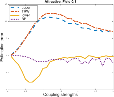
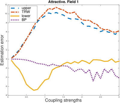
Refer to caption
(a)
Refer to caption
(b)
Figure 4: The attractive case. The (signed) difference of the different bounds and the log-partition function. These experiments illustrate our bounds on 10×10101010\times 10 spin glass model with weak and strong local field potentials and attractive coupling potentials. The plots below zero are lower bounds and plots above zero are upper bounds. We compare our upper bound (35) with the tree re-weighted upper bound. We compare our lower bound (Corollary 4) with the belief propagation result, whose stationary points are known to be lower bounds to the log-partition function for attractive spin-glass models.

We also compared our bound in the mixed case, where the coupling potentials may either be attractive or repulsive, namely θij[c,c]subscript𝜃𝑖𝑗𝑐𝑐\theta_{ij}\in[-c,c]. Recovering the MAP solution in the mixed coupling domain is harder than the attractive domain. Therefore we could not test our lower bound in the mixed setting as it relies on expanding the model. We also omit the comparison to the sum-product belief propagation since it is no longer a lower bound in this setting. We evaluate the MAP perturbation value using MPLP [7]. One can verify that qualitatively the perturb-max upper bound is significantly better than the tree re-weighted upper bound. Nevertheless it is significantly slower as it relies on finding the MAP solution, a harder task in the presence of mixed coupling strengths.
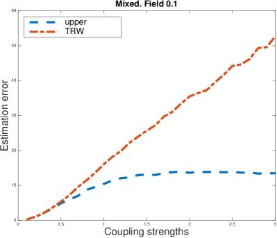
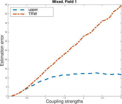
Refer to caption
(a)
Refer to caption
(b)
Figure 5: The (signed) difference of the different bounds and the log-partition function. These experiments illustrate our bounds on 10×10101010\times 10 spin glass model with weak and strong local field potentials and mixed coupling potentials. We compare our upper bound (35) with the tree re-weighted upper bound.

Next, we evaluate the computational complexity of our sampling procedure. Section III-A describes an algorithm that generates unbiased samples from the full Gibbs distribution. For spin glass models with strong local field potentials, it is well-known that one cannot produce unbiased samples from the Gibbs distributions in polynomial time [8, 9, 10]. Theorem 3 connects the computational complexity of our unbiased sampling procedure to the gap between the log-partition function and its upper bound in (35). We use our probable lower bound to estimate this gap on large grids, for which we cannot compute the partition function exactly. Figure 6 suggests that in practice, the running time for this sampling procedure is sub-exponential.
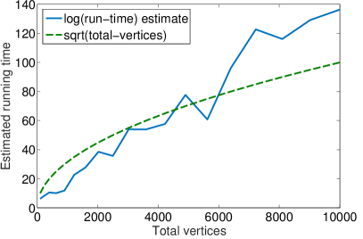
Refer to caption
Figure 6: Estimating our unbiased sampling procedure complexity on spin glass models of varying sizes, ranging from 10×10101010\times 10 spin glass models to 100×100100100100\times 100 spin glass models. The running time is the difference between our upper bound in (35) and the log-partition function. Since the log-partition function cannot be computed for such a large scale model, we replaced it with its lower bound in Corollary 4.

Next we estimate our upper bounds for the entropy of perturb-max probability models that are described in Section III-C. We compare them to marginal entropy bounds H(p)iH(pi)𝐻𝑝subscript𝑖𝐻subscript𝑝𝑖H(p)\leq\sum_{i}H(p_{i}), where pi(xi)=xxip(x)subscript𝑝𝑖subscript𝑥𝑖subscript𝑥subscript𝑥𝑖𝑝𝑥p_{i}(x_{i})=\sum_{x\setminus x_{i}}p(x) are the marginal probabilities [55]. Unlike the log-partition case which relates to the entropy of Gibbs distributions, it is impossible to use dynamic programming to compute the entropy of perturb-max models. Therefore we restrict ourselves to a 4×4444\times 4 spin glass model to compare these upper bounds as shown in Figure 7. One can see that the MAP perturbation upper bound is tighter than the marginalization upper bound in the medium and high coupling strengths. We can also compare the marginal entropy bounds and the perturb-max entropy bounds to arbitrary grid sizes without computing the true entropy. Figure 7 shows that the larger the model the better the perturb-max bound.
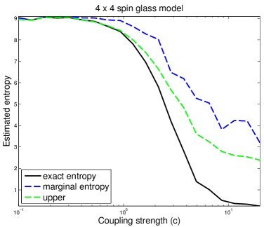
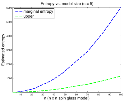
Refer to caption
(a)
Refer to caption
(b)
Figure 7: Estimating our entropy bounds (in Section III-C) while comparing them to the true entropy and the marginal entropy bound. Left: comparison on small-scale spin models. Right: comparison on large-scale spin glass models.

Both our log-partition bounds as well as our entropy bounds hold in expectation. Thus we evaluate their measure concentration properties, i.e., how many samples are required to converge to their expected value. We evaluate our approach on a 100×100100100100\times 100 spin glass model with n=104𝑛superscript104n=10^{4} variables. The local field parameters θisubscript𝜃𝑖\theta_{i} were drawn uniformly at random from [1,1]11[-1,1] to reflect high signal. To find the perturb-max assignment for such a large model we restrict ourselves to attractive coupling setting; the parameters θi,jsubscript𝜃𝑖𝑗\theta_{i,j} were drawn uniformly from [0,c]0𝑐[0,c], where c[0,4]𝑐04c\in[0,4] to reflect weak, medium and strong coupling potentials. Throughout our experiments we evaluate the expected value of our bounds with 100100100 different samples. We note that both our log-partition and entropy upper bounds have the same gradient with respect to their random perturbations, so their measure concentration properties are the same. In the following we only report the concentration of our entropy bounds; the same concentration occurs for our log-partition bounds.

Figure 8 shows the error in the sample mean 1Mj=1MFj1𝑀superscriptsubscript𝑗1𝑀subscript𝐹𝑗\frac{1}{M}\sum_{j=1}^{M}F_{j} as described in Section IV-E. We do so for three different sample sizes M=1,5,10𝑀1510M=1,5,10, while F(γ)=iγi(xiγ)𝐹𝛾subscript𝑖subscript𝛾𝑖subscriptsuperscript𝑥𝛾𝑖F(\gamma)=\sum_{i}\gamma_{i}(x^{\gamma}_{i}) is our entropy bound. The error reduces rapidly as M𝑀M increases; only 101010 samples are needed to estimate the expectation of the perturb-max random function that consist of 104superscript10410^{4} random variables γi(xi)subscript𝛾𝑖subscript𝑥𝑖\gamma_{i}(x_{i}). To test our measure concentration result, that ensures exponential decay, we measure the deviation of the sample mean from its expectation by using M=1,5,10𝑀1510M=1,5,10 samples. Figure 9 shows the histogram of the sample mean, i.e., the number of times that the sample mean has error more than r𝑟r from the true mean. One can see that the decay is indeed exponential for every M𝑀M, and that for larger M𝑀M the decay is much faster. These show that by understanding the measure concentration properties of MAP perturbations, we can efficiently estimate the mean with high probability, even in very high dimensional spin-glass models.
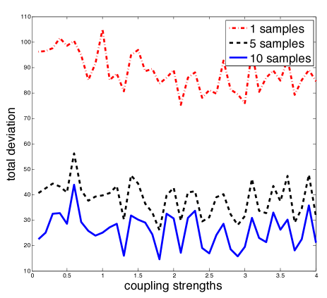
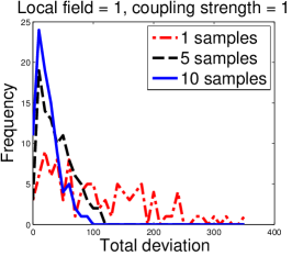
Refer to caption
Figure 8: Error of the sample mean versus coupling strength for 100×100100100100\times 100 spin glass models. The local field parameter θisubscript𝜃𝑖\theta_{i} is chosen uniformly at random from [1,1]11[-1,1] to reflect high signal. With only 101010 samples one can estimate the expectation well.
Refer to caption
(a)
Refer to caption
(b)
Refer to caption
(c)
Figure 9: Histogram that shows the decay of random MAP values, i.e., the number of times that the sample mean has error more than r𝑟r from the true mean. These histograms are evaluated on 100×100100100100\times 100 spin glass model with high signal θi[1,1]subscript𝜃𝑖11\theta_{i}\in[-1,1] and various coupling strengths. One can see that the decay is indeed exponential for every M𝑀M, and that for larger M𝑀M the decay is faster.

Lastly, we demonstrate the effectiveness of MAP perturbations in supervised learning. We consider binary image denoising, which is equivalent to learning the parameters of a spin glass model. The training data was composed of ten 100×7010070100\times 70 binary images, consisting of a man in silhouette corrupted by random binary noise, described in Figure 10. Each image x𝑥x is described by binary local features ϕi(x,yi)subscriptitalic-ϕ𝑖𝑥subscript𝑦𝑖\phi_{i}(x,y_{i}) which equals 111 if the i𝑖i-th pixel of image x𝑥x is foreground and 11-1 otherwise. The pairwise features ϕi,j(yi,yi)=1subscriptitalic-ϕ𝑖𝑗subscript𝑦𝑖subscript𝑦𝑖1\phi_{i,j}(y_{i},y_{i})=1 if yi=yjsubscript𝑦𝑖subscript𝑦𝑗y_{i}=y_{j} and 11-1 otherwise. The goal is to estimate the parameters θi,θi,jsubscript𝜃𝑖subscript𝜃𝑖𝑗\theta_{i},\theta_{i,j} to de-noise the images. The parameters θisubscript𝜃𝑖\theta_{i} determine the importance of background-foreground observations in pixel i𝑖i, and the parameters θi,jsubscript𝜃𝑖𝑗\theta_{i,j} determine the coupling nature of pixels i,j𝑖𝑗i,j, namely their attractive or repulsive strength.

Since we are considering 100×7010070100\times 70 images, there are about 20,0002000020,000 parameters to estimate. Conditional random fields cannot be evaluated on this problem, as the partition function cannot be computed for graphs with many cycles. However, the MAP estimate can be efficiently approximated using MPLP.

Our learning objective function is minθ(x,y)S1|S|𝔼γ[max{iθiϕi(x,yi)+i,jθi,jϕi,j(x,yi,yj)+iγi(yi)}]+θ2subscript𝜃subscript𝑥𝑦𝑆1𝑆subscript𝔼𝛾delimited-[]subscript𝑖subscript𝜃𝑖subscriptitalic-ϕ𝑖𝑥subscript𝑦𝑖subscript𝑖𝑗subscript𝜃𝑖𝑗subscriptitalic-ϕ𝑖𝑗𝑥subscript𝑦𝑖subscript𝑦𝑗subscript𝑖subscript𝛾𝑖subscript𝑦𝑖superscriptnorm𝜃2\min_{\theta}\sum_{(x,y)\in S}\frac{1}{|S|}\mathbb{E}_{\gamma}[\max\{\sum_{i}\theta_{i}\phi_{i}(x,y_{i})+\sum_{i,j}\theta_{i,j}\phi_{i,j}(x,y_{i},y_{j})+\sum_{i}\gamma_{i}(y_{i})\}]+\|\theta\|^{2}, which serves as an upper bound to the Conditional random fields learning objective. When omitting the perturbations this learning objective is the structured-SVM objective (without label loss).

We estimated the expected max-perturbation value by evaluating 555 MAP predictions with random perturbation. We performed gradient decent and stopped either when the gradient step did not improve the objective (decreasing the learning rate by half for 101010 times) or when the algorithm performed 303030 iterations. We compared to structured-SVM by removing the perturbations from our learning algorithm (cf. [67]). Since structured-SVM is a non-smooth program, we used subgradient decent for 10,0001000010,000 iterations and learning rate of 10/T10𝑇10/\sqrt{T}. For completeness, we note that in our previous evaluation, we ran structured-SVM for 303030 iterations and the results were significantly worse [1]. The running time of the learning algorithms is dominated by the number of MAP evaluations, which is 150150150 for learning with random perturbations and 10,0001000010,000 with structured-SVM. To evaluate the two learning algorithms, we used MAP prediction on the test data.555Shpakova and Bach have recently shown that one can improve the test performance by inferring the probabilities of MAP perturbations [68]. When learning with MAP perturbations, the pixel based error on the test set was 1.8%percent1.81.8\%. When learning without perturbations, i.e., with structured-SVMs, the pixel based error on the test set was 2.5%percent2.52.5\%.

Refer to caption Refer to caption Refer to caption Refer to caption model train / test ours SVM-struct

Figure 10: From left to right: (a) Binary 100×7010070100\times 70 image. (b) A representative image in the training set and the test set, where 10%percent1010\% of the pixels are randomly flipped. (c) A de-noised test image with our method: The test set error is 1.8%percent1.81.8\%. (d) A de-noised test image with SVM-struct: The pixel base error is 2.5%percent2.52.5\%.

VI Conclusions

High dimensional inference is a key challenge for applying machine learning in real-life applications. While the Gibbs distribution is widely used throughout many areas of research, standard sampling algorithms may be too slow in many cases of interest. In the last few years many optimization algorithms were devised to avoid the computational burden of sampling and instead researchers predicted the most likely (MAP) solution. In this work we explore novel probability models that rely on MAP optimization as their core element. These models measure the robustness of MAP prediction to random shifts of the potential function. We show how to sample from the Gibbs distribution using the expected value of perturb-max operations. We also derive new entropy bounds for perturb-max models that use the expected value of the maximal perturbations. We complete our exploration by investigating the measure concentration of perturb-max value while showing it can be estimated with only a few perturb-max operations.

The results here can be extended in a number of different directions. In contrast to tree re-weighted or entropy covering bounds, the perturb-max bounds do not have a straightforward tightening scheme. Another direction is to consider the perturb-max model beyond the first moment (expectation). It remains open whether the variance or other related statistics of the perturb-max value can be beneficial for learning, e.g., learning the correlations between data measurements. Understanding the effect of approximate MAP solvers could extend the range of applicability [69, 31]. A natural extension of these methods is to consider high dimensional learning. Perturb-max models already appear implicitly in risk analysis [32] and online learning [33]. Novel approaches that consider perturb-max models explicitly [24, 31] may derive new learning paradigms for high-dimensional inference.

Proof details for Corollary 9

The result in Corollary 9 follows by taking C=4𝐶4C=4 in the following lemma.

Lemma 4

For any a>0𝑎0a>0 and C>0𝐶0C>0, for λ[0,2/aC]𝜆02𝑎𝐶\lambda\in[0,2/a\sqrt{C}]

i=0(1λ2a2C4i+1)2i2+λaC2λaC.superscriptsubscriptproduct𝑖0superscript1superscript𝜆2superscript𝑎2𝐶superscript4𝑖1superscript2𝑖2𝜆𝑎𝐶2𝜆𝑎𝐶\displaystyle\prod_{i=0}^{\infty}\left(1-\frac{\lambda^{2}a^{2}C}{4^{i+1}}\right)^{-2^{i}}\leq\frac{2+\lambda a\sqrt{C}}{2-\lambda a\sqrt{C}}. (77)
Proof:

To prove this inequality there are three simple steps. First, factor out the first term:

i=0(1λ2aaC4i+1)2i=(1λ2a2C4)1i=1(1λ2a2C4i+1)2isuperscriptsubscriptproduct𝑖0superscript1superscript𝜆2superscript𝑎𝑎𝐶superscript4𝑖1superscript2𝑖superscript1superscript𝜆2superscript𝑎2𝐶41superscriptsubscriptproduct𝑖1superscript1superscript𝜆2superscript𝑎2𝐶superscript4𝑖1superscript2𝑖\displaystyle\prod_{i=0}^{\infty}\left(1-\frac{\lambda^{2}a^{a}C}{4^{i+1}}\right)^{-2^{i}}=\left(1-\frac{\lambda^{2}a^{2}C}{4}\right)^{-1}\prod_{i=1}^{\infty}\left(1-\frac{\lambda^{2}a^{2}C}{4^{i+1}}\right)^{-2^{i}} (78)

and define

V(λ)=i=1(1λ2a2C4i+1)2i.𝑉𝜆superscriptsubscriptproduct𝑖1superscript1superscript𝜆2superscript𝑎2𝐶superscript4𝑖1superscript2𝑖\displaystyle V(\lambda)=\prod_{i=1}^{\infty}\left(1-\frac{\lambda^{2}a^{2}C}{4^{i+1}}\right)^{-2^{i}}. (79)

Next, from the identity

(1λ2a2C4)1=4(2+λaC)(2λaC).superscript1superscript𝜆2superscript𝑎2𝐶4142𝜆𝑎𝐶2𝜆𝑎𝐶\displaystyle\left(1-\frac{\lambda^{2}a^{2}C}{4}\right)^{-1}=\frac{4}{(2+\lambda a\sqrt{C})(2-\lambda a\sqrt{C})}. (80)

If we can show that V(λ)<2+λaC2𝑉𝜆2𝜆𝑎𝐶2\sqrt{V(\lambda)}<\frac{2+\lambda a\sqrt{C}}{2} then the result will follow.

We claim V(λ)𝑉𝜆\sqrt{V(\lambda)} is convex. Note that if V(λ)𝑉𝜆V(\lambda) log-convex, then V(λ)𝑉𝜆\sqrt{V(\lambda)} is also convex, so it is sufficient to show that logV(λ)𝑉𝜆\log V(\lambda) is convex. Using the Taylor series expansion log(1x)=j=1xj/j1𝑥superscriptsubscript𝑗1superscript𝑥𝑗𝑗\log(1-x)=-\sum_{j=1}^{\infty}x^{j}/j and switching the order of summation,

logV(λ)𝑉𝜆\displaystyle\log V(\lambda) =i=12ilog(1λ2a2C4i+1)absentsuperscriptsubscript𝑖1superscript2𝑖1superscript𝜆2superscript𝑎2𝐶superscript4𝑖1\displaystyle=-\sum_{i=1}^{\infty}2^{i}\log\left(1-\frac{\lambda^{2}a^{2}C}{4^{i+1}}\right) (81)
=i=12ij=1(λ2a2C)jj4ji+jabsentsuperscriptsubscript𝑖1superscript2𝑖superscriptsubscript𝑗1superscriptsuperscript𝜆2superscript𝑎2𝐶𝑗𝑗superscript4𝑗𝑖𝑗\displaystyle=\sum_{i=1}^{\infty}2^{i}\sum_{j=1}^{\infty}\frac{(\lambda^{2}a^{2}C)^{j}}{j\cdot 4^{ji+j}} (82)
=j=1(λ2a2C)jj4ji=12i2(2j1)iabsentsuperscriptsubscript𝑗1superscriptsuperscript𝜆2superscript𝑎2𝐶𝑗𝑗superscript4𝑗superscriptsubscript𝑖1superscript2𝑖superscript22𝑗1𝑖\displaystyle=\sum_{j=1}^{\infty}\frac{(\lambda^{2}a^{2}C)^{j}}{j4^{j}}\sum_{i=1}^{\infty}\frac{2^{i}}{2^{(2j-1)i}} (83)
=j=1(λ2a2C)jj4j(112(2j1)1)absentsuperscriptsubscript𝑗1superscriptsuperscript𝜆2superscript𝑎2𝐶𝑗𝑗superscript4𝑗11superscript22𝑗11\displaystyle=\sum_{j=1}^{\infty}\frac{(\lambda^{2}a^{2}C)^{j}}{j4^{j}}\left(\frac{1}{1-2^{-(2j-1)}}-1\right) (84)
=j=1(λ2a2C)jj4j(122j11).absentsuperscriptsubscript𝑗1superscriptsuperscript𝜆2superscript𝑎2𝐶𝑗𝑗superscript4𝑗1superscript22𝑗11\displaystyle=\sum_{j=1}^{\infty}\frac{(\lambda^{2}a^{2}C)^{j}}{j4^{j}}\left(\frac{1}{2^{2j-1}-1}\right). (85)

Note that the expansion holds only for λ2a2C4i+1<1superscript𝜆2superscript𝑎2𝐶superscript4𝑖11\frac{\lambda^{2}a^{2}C}{4^{i+1}}<1 and this bound is tightest for i=1𝑖1i=1. This expansion is the sum of convex functions and hence convex. This means that for λ<4aC𝜆4𝑎𝐶\lambda<\frac{4}{a\sqrt{C}} the function V(λ)𝑉𝜆\sqrt{V(\lambda)} is convex.

At λ=2aC𝜆2𝑎𝐶\lambda=\frac{2}{a\sqrt{C}}, we have

logV(2aC)𝑉2𝑎𝐶\displaystyle\log V\left(\frac{2}{a\sqrt{C}}\right) =j=11j(122j11)absentsuperscriptsubscript𝑗11𝑗1superscript22𝑗11\displaystyle=\sum_{j=1}^{\infty}\frac{1}{j}\left(\frac{1}{2^{2j-1}-1}\right) (86)
1+j=21j22j2absent1superscriptsubscript𝑗21𝑗superscript22𝑗2\displaystyle\leq 1+\sum_{j=2}^{\infty}\frac{1}{j\cdot 2^{2j-2}} (87)
=1+4j=2(1/4)jjabsent1superscriptsubscript4𝑗2superscript14𝑗𝑗\displaystyle=1+\frac{4}{\sum}_{j=2}^{\infty}\frac{(1/4)^{j}}{j} (88)
=1+4(log(114)14)absent1411414\displaystyle=1+4\left(-\log\left(1-\frac{1}{4}\right)-\frac{1}{4}\right) (89)
=4log43absent443\displaystyle=4\log\frac{4}{3} (90)
<log4.absent4\displaystyle<\log 4. (91)

Therefore V(2/aC)<4𝑉2𝑎𝐶4V(2/a\sqrt{C})<4.

Since V(0)=1𝑉01V(0)=1 and V(2/aC)<4𝑉2𝑎𝐶4V(2/a\sqrt{C})<4, by convexity, for λ[0,2/aC]𝜆02𝑎𝐶\lambda\in[0,2/a\sqrt{C}],

V(λ)𝑉𝜆\displaystyle\sqrt{V(\lambda)} (1λaC2)V(λ)+λaC2V(2aC)absent1𝜆𝑎𝐶2𝑉𝜆𝜆𝑎𝐶2𝑉2𝑎𝐶\displaystyle\leq\left(1-\frac{\lambda a\sqrt{C}}{2}\right)\sqrt{V(\lambda)}+\frac{\lambda a\sqrt{C}}{2}\sqrt{V\left(\frac{2}{a\sqrt{C}}\right)} (92)
<1+λaC2absent1𝜆𝑎𝐶2\displaystyle<1+\frac{\lambda a\sqrt{C}}{2} (93)
=2+λaC2.absent2𝜆𝑎𝐶2\displaystyle=\frac{2+\lambda a\sqrt{C}}{2}. (94)

Now, considering (78) and the terms in (79) and (80), we have

i=0(1λ2aaC4i+1)2isuperscriptsubscriptproduct𝑖0superscript1superscript𝜆2superscript𝑎𝑎𝐶superscript4𝑖1superscript2𝑖\displaystyle\prod_{i=0}^{\infty}\left(1-\frac{\lambda^{2}a^{a}C}{4^{i+1}}\right)^{-2^{i}} =4(2+λaC)(2λaC)V(λ)absent42𝜆𝑎𝐶2𝜆𝑎𝐶𝑉𝜆\displaystyle=\frac{4}{(2+\lambda a\sqrt{C})(2-\lambda a\sqrt{C})}V(\lambda) (95)
<4(2+λaC)(2λaC)(2+λaC2)2absent42𝜆𝑎𝐶2𝜆𝑎𝐶superscript2𝜆𝑎𝐶22\displaystyle<\frac{4}{(2+\lambda a\sqrt{C})(2-\lambda a\sqrt{C})}\cdot\left(\frac{2+\lambda a\sqrt{C}}{2}\right)^{2} (96)
=2+λaC2λaC,absent2𝜆𝑎𝐶2𝜆𝑎𝐶\displaystyle=\frac{2+\lambda a\sqrt{C}}{2-\lambda a\sqrt{C}}, (97)

as desired. ∎

Acknowledgments

The authors thank the reviewers for their detailed and helpful comments which helped considerably in clarifying the manuscript, Francis Bach and Tatiana Shpakova for helpful discussions, and Associate Editor Constantine Caramanis for his patience and understanding.

References

  • [1] T. Hazan and T. Jaakkola, “On the partition function and random maximum a-posteriori perturbations,” in The 29th International Conference on Machine Learning (ICML 2012), 2012.
  • [2] T. Hazan, S. Maji, and T. Jaakkola, “On sampling from the Gibbs distribution with random maximum a-posteriori perturbations,” in Advances in Neural Information Processing Systems 26, C. Burges, L. Bottou, M. Welling, Z. Ghahramani, and K. Weinberger, Eds.   Curran Associates, Inc., 2013, pp. 1268–1276. [Online]. Available: http://papers.nips.cc/paper/4962-on-sampling-from-the-gibbs-distribution-with-random-maximum-a-posteriori-perturbations
  • [3] F. Orabona, T. Hazan, A. Sarwate, and T. Jaakkola, “On measure concentration of random maximum a-posteriori perturbations,” in Proceedings of The 31st International Conference on Machine Learning, ser. JMLR: Workshop and Conference Proceedings, E. P. Xing and T. Jebara, Eds., vol. 32, 2014, p. 1. [Online]. Available: http://jmlr.csail.mit.edu/proceedings/papers/v32/orabona14.html
  • [4] S. Maji, T. Hazan, and T. Jaakkola, “Active boundary annotation using random MAP perturbations,” in Proceedings of the Seventeenth International Conference on Artificial Intelligence and Statistics (AISTATS), ser. JMLR: Workshop and Conference Proceedings, S. Kaski and J. Corander, Eds., vol. 33, 2014, pp. 604–613. [Online]. Available: http://jmlr.org/proceedings/papers/v33/maji14.html
  • [5] P. F. Felzenszwalb and R. Zabih, “Dynamic programming and graph algorithms in computer vision,” Pattern Analysis and Machine Intelligence, IEEE Transactions on, vol. 33, no. 4, pp. 721–740, April 2011. [Online]. Available: http://dx.doi.org/10.1109/TPAMI.2010.135
  • [6] T. Koo, A. Rush, M. Collins, T. Jaakkola, and D. Sontag, “Dual decomposition for parsing with non-projective head automata,” in Proceedings of the 2010 Conference on Empirical Methods in Natural Language Processing (EMNLP ’10), 2010, pp. 1288–1298. [Online]. Available: http://dl.acm.org/citation.cfm?id=1870783
  • [7] D. Sontag, T. Meltzer, A. Globerson, T. Jaakkola, and Y. Weiss, “Tightening LP relaxations for MAP using message passing,” in Proceedings of the Twenty-Fourth Conference Annual Conference on Uncertainty in Artificial Intelligence (UAI-08).   Corvallis, Oregon, USA: AUAI Press, 2008, pp. 503–510. [Online]. Available: https://dslpitt.org/papers/08/p503-sontag.pdf
  • [8] M. Jerrum and A. Sinclair, “Polynomial-time approximation algorithms for the Ising model,” SIAM Journal on computing, vol. 22, no. 5, pp. 1087–1116, October 1993. [Online]. Available: http://dx.doi.org/10.1137/0222066
  • [9] L. A. Goldberg and M. Jerrum, “The complexity of ferromagnetic Ising with local fields,” Combinatorics Probability and Computing, vol. 16, no. 1, p. 43, January 2007. [Online]. Available: http://dx.doi.org/10.1017/S096354830600767X
  • [10] ——, “Approximating the partition function of the ferromagnetic potts model,” Journal of the ACM (JACM), vol. 59, no. 5, p. 25, 2012.
  • [11] S. Geman and D. Geman, “Stochastic relaxation, Gibbs distributions, and the Bayesian restoration of images,” IEEE Transactions on Pattern Analysis and Machine Intelligence, vol. PAMI-6, no. 6, pp. 721–741, November 1984. [Online]. Available: http://dx.doi.org/10.1109/TPAMI.1984.4767596
  • [12] W. K. Hastings, “Monte Carlo sampling methods using Markov chains and their applications,” Biometrika, vol. 57, no. 1, pp. 97–109, April 1970. [Online]. Available: http://dx.doi.org/10.1093/biomet/57.1.97
  • [13] R. H. Swendsen and J.-S. Wang, “Nonuniversal critical dynamics in Monte Carlo simulations,” Physical Review Letters, vol. 58, no. 2, pp. 86–88, January 1987. [Online]. Available: http://dx.doi.org/10.1103/PhysRevLett.58.86
  • [14] J. M. Eisner, “Three new probabilistic models for dependency parsing: an exploration,” in Proceedings of the 16th Conference on Computational Linguistics (COLING ’96), vol. 1.   Association for Computational Linguistics, 1996, pp. 340–345. [Online]. Available: http://dx.doi.org/10.3115/992628.992688
  • [15] Y. Boykov, O. Veksler, and R. Zabih, “Fast approximate energy minimization via graph cuts,” IEEE Transactions on Pattern Analysis and Machine Intelligence, vol. 23, no. 11, pp. 1222–1239, November 2001. [Online]. Available: http://dx.doi.org/10.1109/34.969114
  • [16] V. Kolmogorov, “Convergent tree-reweighted message passing for energy minimization,” IEEE Transactions on Pattern Analysis and Machine Intelligence, vol. 28, no. 10, pp. 1568–1583, October 2006. [Online]. Available: http://dx.doi.org/10.1109/TPAMI.2006.200
  • [17] Gurobi Optimization. (2015) Gurobi optimizer documentation. [Online]. Available: http://www.gurobi.com/documentation/
  • [18] P. Swoboda, B. Savchynskyy, J. Kappes, and C. Schnörr, “Partial optimality via iterative pruning for the Potts model,” in Scale Space and Variational Methods in Computer Vision: 4th International Conference, ser. Lecture Notes in Computer Science.   Berlin, Germany: Springer, 2013, vol. 7893, ch. 40, pp. 477–488. [Online]. Available: http://dx.doi.org/10.1007/978-3-642-38267-3
  • [19] M. J. Wainwright, T. S. Jaakkola, and A. S. Willsky, “MAP estimation via agreement on trees: Message-passing and linear programming,” IEEE Transactions on Information Theory, vol. 51, no. 11, pp. 3697–3717, November 2005. [Online]. Available: http://dx.doi.org/10.1109/TIT.2005.856938
  • [20] Y. Weiss, C. Yanover, and T. Meltzer, “MAP estimation, linear programming and belief propagation with convex free energies,” in Proceedings of the Twenty-Third Conference Conference on Uncertainty in Artificial Intelligence (2007).   Corvallis, Oregon, USA: AUAI Press, 2007, pp. 416–425. [Online]. Available: https://dslpitt.org/papers/07/p416-weiss.pdf
  • [21] T. Werner, “High-arity interactions, polyhedral relaxations, and cutting plane algorithm for soft constraint optimisation (MAP-MRF),” in Proceedings of the 2008 IEEE Conference on Computer Vision and Pattern Recognition (CVPR), 2008, pp. 1–8. [Online]. Available: http://dx.doi.org/10.1109/CVPR.2008.4587355
  • [22] J. Peng, T. Hazan, N. Srebro, and J. Xu, “Approximate inference by intersecting semidefinite bound and local polytope,” in Proceedings of the Fifteenth International Conference on Artificial Intelligence and Statistics, ser. JMLR: Workshop and Conference Proceedings, N. Lawrence and M. Girolami, Eds., vol. 22, 2012, pp. 868–876. [Online]. Available: http://jmlr.csail.mit.edu/proceedings/papers/v22/peng12.html
  • [23] G. Papandreou and A. Yuille, “Perturb-and-MAP random fields: Using discrete optimization to learn and sample from energy models,” in Proceedings of the 2011 IEEE International Conference on Computer Vision (ICCV), Barcelona, Spain, November 2011, pp. 193–200. [Online]. Available: http://dx.doi.org/10.1109/ICCV.2011.6126242
  • [24] D. Tarlow, R. P. Adams, and R. S. Zemel, “Randomized optimum models for structured prediction,” in Proceedings of the Fifteenth International Conference on Artificial Intelligence and Statistics, ser. JMLR: Workshop and Conference Proceedings, N. Lawrence and M. Girolami, Eds., vol. 22, 2012, pp. 1221–1229. [Online]. Available: http://jmlr.org/proceedings/papers/v22/tarlow12b.html
  • [25] S. Ermon, C. Gomes, A. Sabharwal, and B. Selman, “Taming the curse of dimensionality: Discrete integration by hashing and optimization,” in Proceedings of The 30th International Conference on Machine Learning, ser. JMLR: Workshop and Conference Proceedings, S. Dasgupta and D. McAllester, Eds., vol. 28, no. 2, 2013, pp. 334–342. [Online]. Available: http://jmlr.org/proceedings/papers/v28/ermon13.html
  • [26] ——, “Optimization with parity constraints: From binary codes to discrete integration,” in Proceedings of the Twenty-Ninth Conference Annual Conference on Uncertainty in Artificial Intelligence (UAI-13).   Corvallis, Oregon: AUAI Press, 2013, pp. 202–211.
  • [27] S. Ermon, C. P. Gomes, A. Sabharwal, and B. Selman, “Embed and project: Discrete sampling with universal hashing,” in Advances in Neural Information Processing Systems 26 (NIPS 2013), C. Burges, L. Bottou, M. Welling, Z. Ghahramani, and K. Weinberger, Eds.   Curran Associates, Inc., 2013, pp. 2085–2093. [Online]. Available: http://papers.nips.cc/paper/4965-embed-and-project-discrete-sampling-with-universal-hashing.pdf
  • [28] ——, “Low-density parity constraints for hashing-based discrete integration,” in Proceedings of The 31st International Conference on Machine Learning, ser. JMLR: Workshop and Conference Proceedings, E. P. Xing and T. Jebara, Eds., vol. 32, no. 1, 2014, pp. 271–279. [Online]. Available: http://jmlr.org/proceedings/papers/v32/ermon14.html
  • [29] C. Maddison, D. Tarlow, and T. Minka, “A sampling,” in Advances in Neural Information Processing Systems 27, Z. Ghahramani, M. Welling, C. Cortes, N. Lawrence, and K. Weinberger, Eds.   Curran Associates, Inc., 2014, pp. 2085–2093. [Online]. Available: http://papers.nips.cc/paper/5449-a-sampling
  • [30] G. Papandreou and A. Yuille, “Perturb-and-MAP random fields: Reducing random sampling to optimization, with applications in computer vision,” in Advanced Structured Prediction, S. Nowozin, P. V. Gehler, J. Jancsary, and C. H. Lampert, Eds.   Cambridge, MA, USA: MIT Press, 2014, ch. 7, pp. 159–186.
  • [31] A. Gane and T. S. J. Tamir Hazan, “Learning with maximum a-posteriori perturbation models,” in Proceedings of the Seventeenth International Conference on Artificial Intelligence and Statistics (AISTATS), ser. JMLR: Workshop and Conference Proceedings, S. Kaski and J. Corander, Eds., vol. 33, 2014, pp. 247—256. [Online]. Available: http://jmlr.org/proceedings/papers/v33/gane14.html
  • [32] J. Keshet, D. McAllester, and T. Hazan, “PAC-Bayesian approach for minimization of phoneme error rate,” in Proceedings of the 2011 IEEE International Conference on Acoustics, Speech and Signal Processing (ICASSP), 2011, pp. 2224–2227. [Online]. Available: http://dx.doi.org/10.1109/ICASSP.2011.5946923
  • [33] A. Kalai and S. Vempala, “Efficient algorithms for online decision problems,” Journal of Computer and System Sciences, vol. 71, no. 3, pp. 291–307, October 2005. [Online]. Available: http://dx.doi.org/10.1016/j.jcss.2004.10.016
  • [34] M. Wainwright and M. Jordan, “Graphical models, exponential families, and variational inference,” Foundations and Trends in Machine Learning, vol. 1, no. 1-2, pp. 1–305, 2008. [Online]. Available: http://dx.doi.org/10.1561/2200000001
  • [35] S. Kotz and S. Nadarajah, Extreme value distributions: theory and applications.   London, UK: Imperial College Press, 2000.
  • [36] H. A. David and H. N. Nagaraja, Order Statistics, 3rd ed.   Hoboken, NJ, USA: John Wiley & Sons, 2003.
  • [37] L. G. Valiant, “The complexity of computing the permanent,” Theoretical Computer Science, vol. 8, no. 2, pp. 189–201, 1979. [Online]. Available: http://dx.doi.org/10.1016/0304-3975(79)90044-6
  • [38] V. Kolmogorov and R. Zabih, “What energy functions can be minimized via graph cuts?” IEEE Transactions on Pattern Analysis and Machine Intelligence, vol. 26, no. 2, pp. 147–159, February 2004. [Online]. Available: http://dx.doi.org/10.1109/TPAMI.2004.1262177
  • [39] A. Rush, D. Sontag, M. Collins, and T. Jaakkola, “On dual decomposition and linear programming relaxations for natural language processing,” in Proceedings of the 2010 Conference on Empirical Methods in Natural Language Processing (EMNLP ’10), 2010, pp. 1–11. [Online]. Available: http://dl.acm.org/citation.cfm?id=1870659
  • [40] A. G. Schwing and R. Urtasun, “Efficient exact inference for 3D indoor scene understanding,” in Computer Vision – ECCV 2012 : 12th European Conference on Computer Vision, ser. Lecture Notes in Computer Science.   Berlin, Germany: Springer, 2012, vol. 7577, ch. 22, pp. 299–313. [Online]. Available: http://dx.doi.org/10.1007/978-3-642-33783-3
  • [41] M. Sun, M. Telaprolu, H. Lee, and S. Savarese, “An efficient branch-and-bound algorithm for optimal human pose estimation,” in Proceedings of the 2012 IEEE Conference on Computer Vision and Pattern Recognition (CVPR), Providence, RI, 2012, pp. 1616–1623. [Online]. Available: http://dx.doi.org/10.1109/CVPR.2012.6247854
  • [42] P. Felzenszwalb, R. Girshick, D. McAllester, and D. Ramanan, “Object detection with discriminatively trained part based models,” IEEE Transactions on Pattern Analysis and Machine Intelligence, vol. 32, no. 9, pp. 1627–1645, September 2010. [Online]. Available: http://dx.doi.org/10.1109/TPAMI.2009.167
  • [43] A. Globerson and T. S. Jaakkola, “Fixing max-product: Convergent message passing algorithms for MAP LP-relaxations,” in Advances in Neural Information Processing Systems 20, J. Platt, D. Koller, Y. Singer, and S. Roweis, Eds.   Curran Associates, Inc., 2007, vol. 21, pp. 553–560. [Online]. Available: http://papers.nips.cc/paper/3200-fixing-max-product-convergent-message-passing-algorithms-for-map-lp-relaxations.pdf
  • [44] D. Sontag and T. S. Jaakkola, “New outer bounds on the marginal polytope,” in Advances in Neural Information Processing Systems 20, J. Platt, D. Koller, Y. Singer, and S. Roweis, Eds.   Curran Associates, Inc., 2008, pp. 1393–1400. [Online]. Available: http://papers.nips.cc/paper/3274-new-outer-bounds-on-the-marginal-polytope.pdf
  • [45] R. A. Fisher and L. H. C. Tippett, “Limiting forms of the frequency distribution of the largest or smallest member of a sample,” Mathematical Proceedings of the Cambridge Philosophical Society, vol. 24, no. 02, pp. 180–190, April 1928. [Online]. Available: http://dx.doi.org/10.1017/S0305004100015681
  • [46] B. Gnedenko, “Sur la distribution limite du terme maximum d’une serie aleatoire,” Annals of Mathematics, vol. 44, no. 3, pp. 423–453, July 1943. [Online]. Available: http://dx.doi.org/10.2307/1968974
  • [47] E. J. Gumbel, Statistical theory of extreme values and some practical applications: a series of lectures, ser. National Bureau of Standards Applied Mathematics Series.   Washington, DC, USA: US Govt. Print. Office, 1954, no. 33.
  • [48] R. D. Luce, Individual Choice Behavior: A Theoretical Analysis.   New York, NY, USA: John Wiley and Sons, 1959.
  • [49] M. Ben-Akiva and S. R. Lerman, Discrete Choice Analysis: Theory and Application to Travel Demand.   Cambridge, MA, USA: MIT press, 1985, vol. 9.
  • [50] D. McFadden, “Conditional logit analysis of qualitative choice behavior,” in Frontiers in Econometrics, P. Zarembka, Ed.   New York, NY, USA: Academic Press, 1974, ch. 4, pp. 105–142.
  • [51] G. B. Folland, Real Analysis: Modern Techniques and Their Applications, 2nd ed.   New York, NY, USA: John Wiley & Sons, 2013.
  • [52] D. P. Bertsekas, A. Nedić, and A. E. Ozdaglar, Convex Analysis and Optimization.   Nashua, NH, USA: Athena Scientific, 2003.
  • [53] M. Jordan, Z. Ghahramani, T. Jaakkola, and L. Saul, “An introduction to variational methods for graphical models,” Machine learning, vol. 37, no. 2, pp. 183–233, 1999.
  • [54] M. J. Wainwright, T. S. Jaakkola, and A. S. Willsky, “A new class of upper bounds on the log partition function,” IEEE Transactions on Information Theory, vol. 51, no. 7, pp. 2313–2335, July 2005. [Online]. Available: http://dx.doi.org/10.1109/TIT.2005.850091
  • [55] T. M. Cover and J. A. Thomas, Elements of Information Theory.   Hoboken, NJ, USA: John Wiley & Sons, 2012.
  • [56] H. J. Brascamp and E. H. Lieb, “On extensions of the Brunn-Minkowski and Prékopa-Leindler theorems, including inequalities for log concave functions, and with an application to the diffusion equation,” Journal of Functional Analysis, vol. 22, no. 4, pp. 366–389, August 1976. [Online]. Available: http://dx.doi.org/10.1016/0022-1236(76)90004-5
  • [57] S. Aida, T. Masuda, and I. Shigekawa, “Logarithmic Sobolev inequalities and exponential integrability,” Journal of Functional Analysis, vol. 126, no. 1, pp. 83–101, November 1994. [Online]. Available: http://dx.doi.org/10.1006/jfan.1994.1142
  • [58] S. Bobkov and M. Ledoux, “Poincaré’s inequalities and Talagrand’s concentration phenomenon for the exponential distribution,” Probability Theory and Related Fields, vol. 107, no. 3, pp. 383–400, March 1997. [Online]. Available: http://dx.doi.org/10.1007/s004400050090
  • [59] M. Ledoux, The Concentration of Measure Phenomenon, ser. Mathematical Surveys and Monographs.   American Mathematical Society, 2001, vol. 89.
  • [60] D. Bakry, I. Gentil, and M. Ledoux, Analysis and Geometry of Markov Diffusion Operators, ser. Grundlehren der mathematischen Wissenschaften.   Switzerland: Springer International Publishing, 2014, vol. 348. [Online]. Available: http://dx.doi.org/10.1007/978-3-319-00227-9
  • [61] V. H. Nguyen, “Dimensional variance inequalities of Brascamp–Lieb type and a local approach to dimensional Prékopaʼs theorem,” Journal of Functional Analysis, vol. 266, no. 2, pp. 931–955, January 2014. [Online]. Available: http://dx.doi.org/10.1016/j.jfa.2013.11.003
  • [62] S. G. Bobkov and M. Ledoux, “Weighted Poincaré-type inequalities for Cauchy and other convex measures,” The Annals of Probability, vol. 37, no. 2, pp. 403–427, 2009. [Online]. Available: http://dx.doi.org/10.1214/08-AOP407
  • [63] M. R. Spiegel, S. Lipschutz, and J. Liu, Mathematical Handbook of Formulas and Tables, 4th ed., ser. Schaum’s Outlines.   New York, NY, USA: McGraw-Hill Education, 2013.
  • [64] A. S. Willsky, E. B. Sudderth, and M. J. Wainwright, “Loop series and Bethe variational bounds in attractive graphical models,” in Advances in Neural Information Processing Systems 20, J. Platt, D. Koller, Y. Singer, and S. Roweis, Eds.   Curran Associates, Inc., 2007, pp. 1425–1432. [Online]. Available: http://papers.nips.cc/paper/3354-loop-series-and-bethe-variational-bounds-in-attractive-graphical-models.pdf
  • [65] N. Ruozzi, “The Bethe partition function of log-supermodular graphical models,” in Advances in Neural Information Processing Systems 25, F. Pereira, C. Burges, L. Bottou, and K. Weinberger, Eds.   Curran Associates, Inc., 2012, pp. 117–125. [Online]. Available: http://papers.nips.cc/paper/4649-the-bethe-partition-function-of-log-supermodular-graphical-models.pdf
  • [66] A. Weller and T. Jebara, “Clamping variables and approximate inference,” in Advances in Neural Information Processing Systems 27, Z. Ghahramani, M. Welling, C. Cortes, N. Lawrence, and K. Weinberger, Eds.   Cur, 2014, pp. 909–917. [Online]. Available: http://papers.nips.cc/paper/5529-clamping-variables-and-approximate-inference.pdf
  • [67] I. Tsochantaridis, T. Joachims, T. Hofmann, and Y. Altun, “Large margin methods for structured and interdependent output variables,” Journal of Machine Learning Research, vol. 6, no. 2, p. 1453, 2006.
  • [68] T. Shpakova and F. Bach, “Parameter learning for log-supermodular distributions,” arXiv preprint arXiv:1608.05258, 2016.
  • [69] T. Hazan, S. Maji, J. Keshet, and T. Jaakkola, “Learning efficient random maximum a-posteriori predictors with non-decomposable loss functions,” in Advances in Neural Information Processing Systems 26, C. Burges, L. Bottou, M. Welling, Z. Ghahramani, and K. Weinberger, Eds.   Curran Associates, Inc., 2013, pp. 1887–1895. [Online]. Available: http://papers.nips.cc/paper/4962-on-sampling-from-the-gibbs-distribution-with-random-maximum-a-posteriori-perturbations