The large-scale correlations of multi-cell densities and profiles: implications for cosmic variance estimates

Sandrine Codis1,2, Francis Bernardeau2,3, Christophe Pichon2,4
1 Canadian Institute for Theoretical Astrophysics, University of Toronto, 60 St. George Street, Toronto, ON M5S 3H8, Canada
2 Sorbonne Universités, UPMC Univ Paris 6 & CNRS, UMR 7095, Institut d’Astrophysique de Paris, 98 bis bd Arago, 75014 Paris, France
3 CNRS & CEA, UMR 3681, Institut de Physique Théorique, F-91191 Gif-sur-Yvette, France
4 Korea Institute of Advanced Studies (KIAS) 85 Hoegiro, Dongdaemun-gu, Seoul, 02455, Republic of Korea
codis@cita.utoronto.ca
Abstract

In order to quantify the error budget in the measured probability distribution functions of cell densities, the two-point statistics of cosmic densities in concentric spheres is investigated. Bias functions are introduced as the ratio of their two-point correlation function to the two-point correlation of the underlying dark matter distribution. They describe how cell densities are spatially correlated. They are computed here via the so-called large deviation principle in the quasi-linear regime. Their large-separation limit is presented and successfully compared to simulations for density and density slopes: this regime is shown to be rapidly reached allowing to get sub-percent precision for a wide range of densities and variances. The corresponding asymptotic limit provides an estimate of the cosmic variance of standard concentric cell statistics applied to finite surveys. More generally, no assumption on the separation is required for some specific moments of the two-point statistics, for instance when predicting the generating function of cumulants containing any powers of concentric densities in one location and one power of density at some arbitrary distance from the rest. This exact “one external leg” cumulant generating function is used in particular to probe the rate of convergence of the large-separation approximation.

keywords:
cosmology: theory — large-scale structure of Universe — methods: analytical, numerical

1 Introduction

The geometry of the large-scale structure of the Universe puts very tight constraints on cosmological models. Deep spectroscopic surveys, like Euclid (Laureijs et al., 2011) or DESI (Levi et al., 2013), will soon allow us to study the details of structure formation at different epochs with unrivaled precision and therefore offer insight into the engine of cosmic acceleration. In order to reach percent precision on the equation of state of dark energy, astronomers are facing various challenges: non-linear gravitational evolution (Bernardeau et al., 2002), redshift space distortions (Kaiser, 1987; Taruya et al., 2010), bias (Kaiser, 1984; Dekel & Rees, 1987), intrinsic alignments (Kiessling et al., 2015), baryonic physics (Schneider & Teyssier, 2015) to name a few. Probing the non-linear regime increases the number of modes used to better constrain cosmological parameters. Hence, theorists need to investigate alternatives to the standard N-point correlation functions (Scoccimarro et al., 1998) that Perturbation Theory can only predict in the weakly non-linear regime (Lazanu et al., 2015). They must find new observables that can be predicted from first principles, and do not rely solely on very large simulations of the Universe produced with hundreds of millions of CPU hours.

It has been argued (Bernardeau et al., 2014, 2015; Uhlemann et al., 2015) that the statistics of cosmic densities in concentric spheres can leverage cosmic parameters competitively, as the corresponding spherical symmetry allows for analytical predictions in the mildly non-linear regime, beyond what is commonly achievable via other statistics such as correlation functions. Indeed, the zero variance limit of the cumulant generating functions yields estimates of the joint probability distribution function (PDF hereafter) which seems to match simulations in the regime of variances of order unity as shown by Valageas (2002); Bernardeau et al. (2014, 2015) building upon some earlier investigations by Balian & Schaeffer (1989); Bernardeau (1992). This success has been recently shown to correspond to a large-deviation principle in the context of cosmic structure formation (Bernardeau & Reimberg, 2015) which is based on the sole assumption that the variance of the field is small. The corresponding predictions for the successive reduced cumulants were shown to be in excellent agreement with simulations for scale above a few Mpc/habsent/h (e.g Baugh et al. (1995)). It has to be contrasted with the commonly used polyspectra predicted by Perturbation Theory which typically require the fluctuations of the field to be small everywhere. For instance, unless large-deviation predictions, the Edgeworth expansion typically breaks down for |δ|>σ𝛿𝜎|\delta|>\sigma.

Hence it is of interest to quantify the error budget for such large-deviation estimators, while accounting for the expected long-range clustering within realistic surveys of finite extent. Indeed, in practice, measurements of cosmic densities cannot be carried out for different realisations i.e different universes but in one finite part of our Universe as mapped by surveys like the SDSS (Abazajian et al., 2003) or DES (Sánchez et al., 2014). The density in spheres drawn from those surveys are not independent. Consequently, this dependence induces errors which, at first order, are dominated by the two-point correlation between spheres, as shown by Maurogordato & Lachieze-Rey (1987); Colombi et al. (1995); Szapudi & Colombi (1996); Moster et al. (2011). Estimating the two-point correlations of concentric cosmic densities (Bernardeau, 1996; Szapudi et al., 1999) is therefore important to mitigate the cosmic variance on the measurement of their one-point statistics. Once a model for these correlations exists, it can be integrated into maximum likelihood estimators for the underlying cosmic parameters.

Besides error statistics, the study of this two-point clustering statistics of concentric spheres is also interesting in its own right, as it allows one to investigate how the densest regions of space – where dark halos usually reside – are clustered in the quasi-linear regime, which in turn sheds light on the so-called biasing between dark matter and halos: a common, apparently good assumption (Ludlow & Porciani, 2011), is that haloes correspond to peaks of the density field, they are therefore not a fair tracer of that field. For Gaussian random fields, Kaiser (1984) showed that in the high contrast ν𝜈\nu, high separation limit, the correlation function, ξ>νsubscript𝜉absent𝜈\xi_{>\nu}, between two regions lying above a threshold ν𝜈\nu reads

ξ>νν2ξ,subscript𝜉absent𝜈superscript𝜈2𝜉\xi_{>\nu}\approx\nu^{2}\xi, (1)

so that the correlation function of high-density regions decreases more slowly than the density field correlation function, ξ𝜉\xi, with an amplification factor or clustering bias that is proportional to the threshold squared. This analysis can also be restricted to the peaks of the density field above a given threshold following the seminal paper by Bardeen et al. (1986).

Building upon the idea that the density of large clusters must be strongly clustered compared to the density of galaxies, Davis et al. (1985) popularized the notion of linear bias between the galaxy distribution and dark matter density field

δg=b1δDM,subscript𝛿gsubscript𝑏1subscript𝛿DM\delta_{\mathrm{g}}=b_{1}\delta_{\rm DM}\,, (2)

where b1subscript𝑏1b_{1} is assumed to be a constant which was shown to be a good approximation on sufficiently large scales (Manera & Gaztañaga, 2011). However, given the complexity of galaxy formation, the validity of this approximation is likely to be somewhat narrow. Fry & Gaztañaga (1993) proposed to extend the linear bias approach and to introduce the so-called local bias model in which the full Taylor expansion of the relation δg=(δDM)subscript𝛿𝑔subscript𝛿DM\delta_{g}={\cal F}(\delta_{\rm DM}) is considered. This parametrization can be studied from a Eulerian or a Lagrangian point of view, meaning at final or initial time, (Catelan et al., 2000) and can account for stochasticity (Dekel & Lahav (1999)), time-evolution (Nusser & Davis (1994); Fry (1996); Tegmark & Peebles (1998)), non-linearity (Pen (1998); Guo & Jing (2009)), scale-dependence (Lumsden et al. (1989); Giannantonio & Porciani (2010)) or non-locality in time (Senatore, 2015). Non-local effects can also be addressed by parametrizing the dependence of the galaxy density with other operators such as the tidal tensor or velocity shear as long as they preserve the symmetry and equivalence (McDonald & Roy, 2009; Baldauf et al., 2012; Mirbabayi et al., 2015). De facto, this bias is very likely to depend on the population of galaxies and to be not only a function of the density but also temperature, merging history and other galaxy properties, introducing some scatter in the galaxy-matter density relation. Quantifying bias is crucial in cosmology if one wants to measure the cosmological parameters encoded in ξ𝜉\xi from, e.g. the correlation function of galaxies. It is also an interesting quantity to measure in its own right, as it carries information on the physics of galaxy formation. Numerical simulations are very efficient at accurately predicting and calibrating galactic observables. Improvements of our understanding of galaxy formation and its implementation in simulations is a timely and fast moving topic of research.

However, it has to be noted that the scale-dependence of the halo bias (defined as the ratio of the halo-halo to dark matter correlation functions) is strong on small scales but remains weak with typical deviations of less than a few percents on scales above 20 Mpc/h (Crocce et al., 2015). It would therefore be interesting to predict the bias of specific regions (for instance high density and/or negative slope as a proxy for dark halos) from first principles not only in the linear stage of structure formation but also in the subsequent mildly non-linear regime.

The aim of this paper is to quantify the effect of cosmic variance on count-in-cells statistics in the mildly non-linear regime. Specifically we will estimate the two-point correlations of concentric cosmic densities at different positions in the field in the (not so) large separation limit, while relying on the symmetric framework of the spherical collapse, which leads to surprisingly accurate predictions. It will allow us in particular to define the bias associated with concentric cosmic densities and provide accurate predictions up to a few Mpc/habsent/h.

This paper is organized as follows. Section 2 predicts the bias and error budget expected in standard concentric count-in-cells. Section 3 shows how to compute the generating function of the cumulants containing any power of the densities in one location and one power of the density at an arbitrary distance. Section 4 predicts the bias functions in the large separation limit while section 5 applies the formalism to realistic power spectra. Section 6 validates this large-separation and large-deviation approximation on simulations before Section 7 illustrates how bias functions can be used to predict the expected error budget when estimating the PDF of the cosmic density in concentric spheres. Finally, Section 8 wraps up. Appendices A, B, C, D, E and F respectively present the radii decimation used in the main text, an argument in favour of the large-distance factorizations, some calculations of cosmic variance for discrete counts, a consistency check of the measurements of the bias function by two distinct methods and analytical asymptotes for the density and slope bias.

2 Statistics of sets of count-in-cells

In a survey or a simulation, measurements of concentric densities are carried as follows: sets of concentric cells are drawn randomly or regularly across the field at some finite distance to each other. In cosmology, this field has long-range correlations which will break the assumption that each set of concentric spheres can be considered independently. In order to estimate the induced bias and variance, let us study the joint statistics of these sets.

2.1 The bias function of concentric spheres
Refer to caption
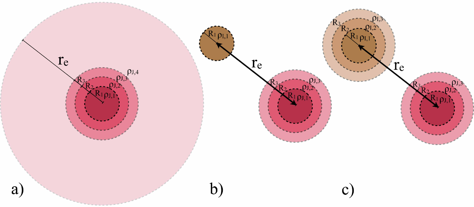
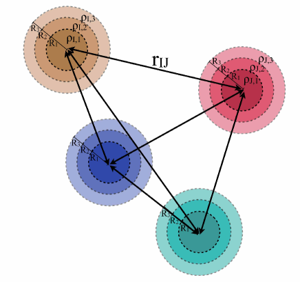
Figure 1: The configuration of spherical cells considered in this paper which is made of multiple sets of concentric spheres separated by distances rIJsubscript𝑟IJr_{\rm{IJ}}. Their respective density, ρI,isubscript𝜌Ii\rho_{\rm{I},i}, corresponds to a set of n𝑛n spheres of same radii RI,iRisubscript𝑅Iisubscript𝑅𝑖R_{\rm I,i}\equiv R_{i}.

Let us consider multiple sets (labelled from I=1I1\rm I=1 to NtsubscriptNt\rm N_{t}) of n𝑛n concentric spheres (labelled from k=1𝑘1k=1 to n𝑛n) of radii RI,kRksubscript𝑅Iksubscript𝑅𝑘R_{\rm I,k}\equiv R_{k} separated by distances rIJsubscript𝑟IJr_{\rm{IJ}}, and define the corresponding measured densities {ρI,k}subscript𝜌Ik\{\rho_{\rm I,k}\} (see Fig. 1 for an illustration). The joint PDF of those NtsubscriptNt\rm N_{t} sets,

𝒫({ρ1,k},,{ρNt,k};{rIJ}),𝒫subscript𝜌1𝑘subscript𝜌subscriptNt𝑘subscript𝑟IJ{\cal P}(\{\rho_{1,k}\},\dots,\{\rho_{{\rm N_{t}},k}\};\{r_{\rm{IJ}}\})\,, (3)

determines the full hierarchy of cumulants of the form

ρ1,1p1ρ1,npnρ2,1q1ρ2,nqnρNt,1s1ρNt,nsnc.subscriptdelimited-⟨⟩superscriptsubscript𝜌11subscript𝑝1superscriptsubscript𝜌1𝑛subscript𝑝𝑛superscriptsubscript𝜌21subscript𝑞1superscriptsubscript𝜌2𝑛subscript𝑞𝑛superscriptsubscript𝜌subscriptNt1subscript𝑠1superscriptsubscript𝜌subscriptNt𝑛subscript𝑠𝑛𝑐\langle\rho_{1,1}^{p_{1}}\dots\rho_{1,n}^{p_{n}}{\rho_{2,1}^{q_{1}}}\dots\rho_{2,n}^{q_{n}}\dots\rho_{\rm{{N_{t}}},1}^{s_{1}}\dots\rho_{{\rm{N_{t}}},n}^{s_{n}}\rangle_{c}\,. (4)

The purpose of this paper is to estimate the joint PDF 𝒫({ρ1,k},,{ρNt,k};{rIJ})){\cal P}(\{\rho_{1,k}\},\dots,\{\rho_{\rm{N_{t}},k}\};\{r_{\rm{IJ}}\})) in the large-separation limit, where rIJRmax=maxjRjmuch-greater-thansubscript𝑟IJsubscript𝑅maxsubscript𝑗subscript𝑅𝑗r_{\rm{IJ}}\gg R_{\mathrm{max}}=\max_{j}R_{j}. In this limit, we will demonstrate in Section 4.2 that this PDF reads

𝒫(\displaystyle{\cal P}( {ρ1,k},,{ρNt,k};{rIJ}Rj)=\displaystyle\{\rho_{1,k}\},\dots,\{\rho_{{\rm N_{t}},k}\};\{r_{\rm{IJ}}\}\gg R_{j})=
I=1Nt𝒫({ρI,k})[1+I<Jb({ρI,k})b({ρJ,k})ξ(rIJ)],superscriptsubscriptproductI1subscriptNt𝒫subscript𝜌I𝑘delimited-[]1subscriptIJ𝑏subscript𝜌I𝑘𝑏subscript𝜌J𝑘𝜉subscript𝑟IJ\displaystyle\prod_{\rm I=1}^{\rm{N_{t}}}{\cal P}(\{\rho_{{\rm I},k}\})\left[1+\ \sum_{\rm{I<J}}b(\{\rho_{{\rm I},k}\})b(\{\rho_{{\rm J},k}\})\xi(r_{\rm{IJ}})\right]\,, (5)

where ΠI𝒫({ρI,k})subscriptΠI𝒫subscript𝜌I𝑘\Pi_{\rm I}{\cal P}(\{\rho_{{\rm I},k}\}) is the product of one-point PDFs, ξ(r)𝜉𝑟\xi(r) is the underlying dark matter correlation function, and b({ρI,k})𝑏subscript𝜌I𝑘b(\{\rho_{{\rm I},k}\}) is some local bias function for the set I of n𝑛n concentric spheres. This is the count-in-cell analog of the so-called peak-background-split or clustering bias. Equation (5) is the key result of this paper and will be used in the following sections to compute b({ρI,k})𝑏subscript𝜌I𝑘b(\{\rho_{{\rm I},k}\}) whose final expression is given by equations (36) and (42) below. We will also show in Section 4.4 that the bias obeys b(ρ)𝒫(ρ)dρ=0𝑏𝜌𝒫𝜌d𝜌0\int b(\rho){\cal P}(\rho)\hbox{d}\rho=0 and ρb(ρ)𝒫(ρ)dρ=1𝜌𝑏𝜌𝒫𝜌d𝜌1\int\rho\,b(\rho){\cal P}(\rho)\hbox{d}\rho=1 so that the N-point PDF given in equation (5) is normalised and its marginal in one location is exactly given by the one-point PDF.

Equation (5) allows us to define the excess probability of having the sets of densities {ρ1,k},,{ρNt,k}subscript𝜌1𝑘subscript𝜌subscriptNt𝑘\{\rho_{{1},k}\},\dots,\{\rho_{{\rm N_{t}},k}\} separated by {rIJ}subscript𝑟IJ\left\{r_{\mathrm{IJ}}\right\} as

ξNt({ρ1,k},,{ρNt,k})=I<Jb({ρI,k})b({ρJ,k})ξ(rIJ).subscript𝜉subscriptNtsubscript𝜌1𝑘subscript𝜌subscriptNt𝑘subscriptIJ𝑏subscript𝜌I𝑘𝑏subscript𝜌J𝑘𝜉subscript𝑟IJ\xi_{\rm N_{t}}(\{\rho_{1,k}\},\dots,\{\rho_{{\rm N_{t}},k}\})=\sum_{\mathrm{I<J}}b(\{\rho_{{\rm I},k}\})b(\{\rho_{{\rm J},k}\})\xi(r_{\rm IJ}). (6)

From equation (6), we see that the error in assuming that the draws of concentric densities in simulations are independent scales like the dark matter correlation111 In analogy with the corresponding situation for peaks, we can anticipate corrections involving derivative of the dark matter correlation at shorter separations..

2.2 The bias and variance of concentric cumulants

Let us now define the arithmetic mean over sets of concentric spheres as

ρ1p1ρnpn¯1NtIρI,1p1ρI,npn.¯superscriptsubscript𝜌1subscript𝑝1superscriptsubscript𝜌𝑛subscript𝑝𝑛1subscriptNtsubscriptIsuperscriptsubscript𝜌I1subscript𝑝1superscriptsubscript𝜌I𝑛subscript𝑝𝑛\overline{\rho_{1}^{p_{1}}\dots\rho_{n}^{p_{n}}}\equiv\frac{1}{\rm N_{t}}\sum_{\mathrm{I}}\rho_{\mathrm{I},1}^{p_{1}}\dots\rho_{\mathrm{I},n}^{p_{n}}\,. (7)

This quantity naturally corresponds to what astronomers would measure in practice (spatial averages rather than ensemble averages). Our purpose is to quantify the bias and the expected cosmic variance of this estimator. Given equation (5), one can check that the expectation of the arithmetic estimator defined by equation (7) obeys

ρ1p1ρnpn¯c=ρ1p1ρnpnc,subscriptdelimited-⟨⟩¯superscriptsubscript𝜌1subscript𝑝1superscriptsubscript𝜌𝑛subscript𝑝𝑛𝑐subscriptdelimited-⟨⟩superscriptsubscript𝜌1subscript𝑝1superscriptsubscript𝜌𝑛subscript𝑝𝑛𝑐\langle\overline{\rho_{1}^{p_{1}}\dots\rho_{n}^{p_{n}}}\rangle_{c}=\langle{\rho_{1}^{p_{1}}\dots\rho_{n}^{p_{n}}}\rangle_{c}\,, (8)

so that the mean of the estimator given by equation (7) is unbiased at large distances.

Let us now estimate the cross correlation of this estimator, C𝐩𝐪ρ1p1ρnpn¯ρ1q1ρnqn¯csubscript𝐶𝐩𝐪subscriptdelimited-⟨⟩¯superscriptsubscript𝜌1subscript𝑝1superscriptsubscript𝜌𝑛subscript𝑝𝑛¯superscriptsubscript𝜌1subscript𝑞1superscriptsubscript𝜌𝑛subscript𝑞𝑛𝑐C_{\mathbf{p}\mathbf{q}}\equiv\langle\overline{\rho_{1}^{p_{1}}\dots\rho_{n}^{p_{n}}}\,\overline{\rho_{1}^{q_{1}}\dots\rho_{n}^{q_{n}}}\rangle_{c} and express it in terms of moments of the bias function

C𝐩𝐪=1Ntρ1p1+q1ρnpn+qnc+1Nt2IJξ(rIJ)×b(ρ1ρn)ρ1p1ρnpncb(ρ1ρn)ρ1q1ρnqnc.subscript𝐶𝐩𝐪1subscriptNtsubscriptdelimited-⟨⟩superscriptsubscript𝜌1subscript𝑝1subscript𝑞1superscriptsubscript𝜌𝑛subscript𝑝𝑛subscript𝑞𝑛𝑐1superscriptsubscriptNt2subscriptIJ𝜉subscript𝑟IJsubscriptdelimited-⟨⟩𝑏subscript𝜌1subscript𝜌𝑛superscriptsubscript𝜌1subscript𝑝1superscriptsubscript𝜌𝑛subscript𝑝𝑛𝑐subscriptdelimited-⟨⟩𝑏subscript𝜌1subscript𝜌𝑛superscriptsubscript𝜌1subscript𝑞1superscriptsubscript𝜌𝑛subscript𝑞𝑛𝑐C_{\mathbf{p}\mathbf{q}}=\frac{1}{\mathrm{N_{t}}}\left\langle\rho_{1}^{p_{1}+q_{1}}\dots\rho_{n}^{p_{n}+q_{n}}\right\rangle_{c}+\frac{1}{\mathrm{N_{t}}^{2}}\sum_{\rm I\neq J}\xi(r_{\mathrm{IJ}})\times\\ \left\langle b(\rho_{1}\!\dots\!\rho_{n})\rho_{1}^{p_{1}}\!\dots\!\rho_{n}^{p_{n}}\right\rangle_{c}\left\langle b(\rho_{1}\!\dots\!\rho_{n})\rho_{1}^{q_{1}}\!\dots\!\rho_{n}^{q_{n}}\right\rangle_{c}\,. (9)

The first term in equation (9) is the error on the mean which is the typical error if draws are independent. The correlations between the draws – i.e the cells – lead to an additional source of errors encoded in the second term which corresponds to the bias function. Note that as expected, in the very large separation limit where ξ(rIJ)δIJ𝜉subscript𝑟IJsubscript𝛿IJ\xi(r_{\mathrm{IJ}})\rightarrow\delta_{\mathrm{IJ}}, we get C𝐩𝐪C𝐩𝐪0/Ntsubscript𝐶𝐩𝐪subscriptsuperscript𝐶0𝐩𝐪subscriptNtC_{\mathbf{p}\mathbf{q}}\rightarrow C^{0}_{\mathbf{p}\mathbf{q}}/\mathrm{N_{t}} where C𝐩𝐪0=ρ1p1+q1ρnpn+qncsubscriptsuperscript𝐶0𝐩𝐪subscriptdelimited-⟨⟩superscriptsubscript𝜌1subscript𝑝1subscript𝑞1superscriptsubscript𝜌𝑛subscript𝑝𝑛subscript𝑞𝑛𝑐C^{0}_{\mathbf{p}\mathbf{q}}=\left\langle\rho_{1}^{p_{1}+q_{1}}\dots\rho_{n}^{p_{n}+q_{n}}\right\rangle_{c} and δIJsubscript𝛿IJ\delta_{\mathrm{IJ}} is the Kronecker delta function here.

2.3 Errors on the PDF

Let us finally quantify the cosmic variance on the estimate of the one-cell PDF when measuring densities in a finite number NtsubscriptNt\rm N_{t} of spheres. In this case, it is necessary to take into account the discreteness of the counts and the size of the bins of density.

One can show (see Appendix C for details) that in the Poisson limit, the number NN\rm N of spheres with density in the interval Δ=[ρΔρ/2,ρ+Δρ/2]Δ𝜌Δ𝜌2𝜌Δ𝜌2\Delta=[\rho-\Delta\rho/2,\rho+\Delta\rho/2] is unbiased (N=N¯delimited-⟨⟩N¯𝑁\left\langle\rm N\right\rangle=\bar{N}) and has variance

N2N2=N¯+b2ξN¯2,delimited-⟨⟩superscriptN2superscriptdelimited-⟨⟩N2¯Nsuperscript𝑏2𝜉superscript¯N2\left\langle\rm N^{2}\right\rangle-\left\langle\rm N\right\rangle^{2}={\rm\bar{N}}+b^{2}\xi\rm\bar{N}^{2}\,, (10)

where ξ𝜉\xi is the mean correlation between the spheres, ξ=IJξ(rIJ)/[Nt(Nt1)]𝜉subscriptIJ𝜉subscript𝑟IJdelimited-[]subscriptNtsubscriptNt1\xi=\sum_{\rm I\neq J}\xi(r_{\rm IJ})/[\rm N_{t}(N_{t}-1)], and N¯=pNt¯N𝑝subscriptNt{\rm\bar{N}}=p\rm N_{t} with p=Δdρ𝒫(ρ)𝑝subscriptΔd𝜌𝒫𝜌p=\int_{\Delta}\hbox{d}\rho{\cal P}(\rho) is the expected number of spheres with density in the interval considered. For a large enough number of spheres, sampling errors can therefore be neglected and the cosmic variance is directly proportional to b2superscript𝑏2b^{2} where here b𝑏b is defined as the mean density bias in the bin

b=Δ𝒫(ρ)b(ρ)dρ/Δ𝒫(ρ)dρ,𝑏subscriptΔ𝒫𝜌𝑏𝜌d𝜌subscriptΔ𝒫𝜌d𝜌b=\int_{\Delta}{\cal P}(\rho)b(\rho)\hbox{d}\rho/\int_{\Delta}{\cal P}(\rho)\hbox{d}\rho\,, (11)

where the density bias, b(ρ)𝑏𝜌b(\rho), entering equation (5) will later be shown to obey equation (42).

Similarly, the correlations between the counts in different bins of density can be investigated. The numbers N1subscriptN1\rm N_{1} of spheres with density in Δ1=[ρ1Δρ/2,ρ1+Δρ/2]subscriptΔ1subscript𝜌1Δ𝜌2subscript𝜌1Δ𝜌2\Delta_{1}=[\rho_{1}-\Delta\rho/2,\rho_{1}+\Delta\rho/2] and N2subscriptN2\rm N_{2} of spheres with density in Δ2=[ρ2Δρ/2,ρ2+Δρ/2]subscriptΔ2subscript𝜌2Δ𝜌2subscript𝜌2Δ𝜌2\Delta_{2}=[\rho_{2}-\Delta\rho/2,\rho_{2}+\Delta\rho/2] are unbiased and have a covariance

N1N2=N¯1N¯2(1+ξb1b2),delimited-⟨⟩subscriptN1subscriptN2subscript¯N1subscript¯N21𝜉subscript𝑏1subscript𝑏2\left\langle\rm N_{1}N_{2}\right\rangle={\rm\bar{N}_{1}\bar{N}_{2}}(1+\xi b_{1}b_{2})\,, (12)

with b1subscript𝑏1b_{1} and b2subscript𝑏2b_{2} being defined as in equation (11) for the bins ρ1±Δρ/2plus-or-minussubscript𝜌1Δ𝜌2\rho_{1}\pm\Delta\rho/2 and ρ^2±Δρ/2plus-or-minussubscript^𝜌2Δ𝜌2\hat{\rho}_{2}\pm\Delta\rho/2. The proof of this result is again derived in Appendix C and can be easily generalized to any number of concentric cells.

The consequence for the error budget of the one-cell PDF is as follows. Let us define 𝒫^(ρi)=Ni/Nt/Δρ^𝒫subscript𝜌𝑖subscriptNisubscriptNtΔ𝜌\hat{\cal P}(\rho_{i})={\rm N_{i}/N_{t}}/\Delta\rho, the estimate of the PDF measured from a set of NtsubscriptNt\rm N_{t} spheres when the range of densities is divided in bins centred on ρisubscript𝜌𝑖\rho_{i} with width ΔρΔ𝜌\Delta\rho. First, this estimator, 𝒫^^𝒫\hat{\cal P}, is unbiased. Equations (10) and (12) also yield the expected error on the estimate of the PDF

𝒫^(ρi)2𝒫^(ρi)2=𝒫¯(ρi)ΔρNt+bi2ξ(𝒫¯(ρi))2,delimited-⟨⟩^𝒫superscriptsubscript𝜌𝑖2superscriptdelimited-⟨⟩^𝒫subscript𝜌i2¯𝒫subscript𝜌𝑖Δ𝜌subscriptNtsuperscriptsubscript𝑏𝑖2𝜉superscript¯𝒫subscript𝜌𝑖2\left\langle\hat{\cal P}(\rho_{i})^{2}\right\rangle-\left\langle\rm\hat{\cal P}(\rho_{i})\right\rangle^{2}=\frac{\bar{\cal P}(\rho_{i})}{\Delta\rho\rm N_{t}}+b_{i}^{2}\xi\left(\bar{\cal P}(\rho_{i})\right)^{2}\,, (13)

where the mean PDF in the bin is 𝒫¯(ρi)=Δi𝒫(ρ)dρ/Δρ¯𝒫subscript𝜌𝑖subscriptsubscriptΔ𝑖𝒫𝜌d𝜌Δ𝜌\bar{\cal P}(\rho_{i})=\int_{\Delta_{i}}{\cal P}(\rho)\hbox{d}\rho/\Delta\rho and bi2(𝒫¯(ρi))2superscriptsubscript𝑏𝑖2superscript¯𝒫subscript𝜌𝑖2b_{i}^{2}\left(\bar{\cal P}(\rho_{i})\right)^{2} is the mean value squared of the bias in the density bin, (Δi𝒫(ρ)b(ρ)dρ/Δρ)2superscriptsubscriptsubscriptΔ𝑖𝒫𝜌𝑏𝜌d𝜌Δ𝜌2\left(\int_{\Delta_{i}}{\cal P}(\rho)b(\rho)\hbox{d}\rho/\Delta\rho\right)^{2}. Furthermore, the typical correlation between two distinct bins, ij𝑖𝑗i\neq j, is given by

𝒫^(ρi)𝒫^(ρj)=𝒫¯(ρi)𝒫¯(ρj)(1+ξbibj).delimited-⟨⟩^𝒫subscript𝜌𝑖^𝒫subscript𝜌𝑗¯𝒫subscript𝜌𝑖¯𝒫subscript𝜌𝑗1𝜉subscript𝑏𝑖subscript𝑏𝑗\left\langle\hat{\cal P}(\rho_{i})\hat{\cal P}(\rho_{j})\right\rangle=\bar{\cal P}(\rho_{i})\bar{\cal P}(\rho_{j})(1+\xi b_{i}b_{j})\,. (14)

In particular, it is straightforward to see that equation (14) is fully consistent with equation (9) in the one-cell case. Indeed, from equations (14) and  (13), one can compute for instance the correlation between the estimated moment of order p𝑝p of the density and the moment of order q𝑞q

Mpqsubscript𝑀𝑝𝑞\displaystyle M_{pq} =ρp¯ρq¯,absentdelimited-⟨⟩¯superscript𝜌𝑝¯superscript𝜌𝑞\displaystyle\!=\!\left\langle\overline{\rho^{p}}\,\overline{\rho^{q}}\right\rangle,
=i,j(Δρ)2𝒫^(ρi)𝒫^(ρj)ρipρjq,absentsubscript𝑖𝑗superscriptΔ𝜌2delimited-⟨⟩^𝒫subscript𝜌𝑖^𝒫subscript𝜌𝑗superscriptsubscript𝜌𝑖𝑝superscriptsubscript𝜌𝑗𝑞\displaystyle\!=\!\sum_{i,j}(\Delta\rho)^{2}\left\langle\hat{\cal P}(\rho_{i})\hat{\cal P}(\rho_{j})\right\rangle\rho_{i}^{p}\rho_{j}^{q},
=i,j(Δρ)2𝒫¯(ρi)𝒫¯(ρj)(1+ξbibj)ρipρjq+iΔρNtρip+q𝒫¯(ρ^i),absentsubscript𝑖𝑗superscriptΔ𝜌2¯𝒫subscript𝜌𝑖¯𝒫subscript𝜌𝑗1𝜉subscript𝑏𝑖subscript𝑏𝑗superscriptsubscript𝜌𝑖𝑝superscriptsubscript𝜌𝑗𝑞subscript𝑖Δ𝜌subscriptNtsuperscriptsubscript𝜌𝑖𝑝𝑞¯𝒫subscript^𝜌𝑖\displaystyle\!=\!\sum_{i,j}(\Delta\rho)^{2}\bar{\cal P}(\rho_{i})\bar{\cal P}(\rho_{j})(1\!+\!\xi b_{i}b_{j})\rho_{i}^{p}\rho_{j}^{q}\!+\!\!\sum_{i}\!\!\frac{\Delta\rho}{\rm N_{t}}\rho_{i}^{p+q}\bar{\cal P}({\hat{\rho}}_{i}),
=1Ntρp+q+ρpρq+ξb(ρ)ρpb(ρ)ρq,absent1subscriptNtdelimited-⟨⟩superscript𝜌𝑝𝑞delimited-⟨⟩superscript𝜌𝑝delimited-⟨⟩superscript𝜌𝑞𝜉delimited-⟨⟩𝑏𝜌superscript𝜌𝑝delimited-⟨⟩𝑏𝜌superscript𝜌𝑞\displaystyle\!=\!\frac{1}{\rm N_{t}}\left\langle\rho^{p+q}\right\rangle+\left\langle\rho^{p}\right\rangle\left\langle\rho^{q}\right\rangle+\xi\left\langle b(\rho)\rho^{p}\right\rangle\left\langle b(\rho)\rho^{q}\right\rangle,

which in terms of cumulants can be rewritten as

Cpq=ρp¯ρq¯c=1Ntρp+qc+ξb(ρ)ρpcb(ρ)ρqc,subscript𝐶𝑝𝑞subscriptdelimited-⟨⟩¯superscript𝜌𝑝¯superscript𝜌𝑞𝑐1subscriptNtsubscriptdelimited-⟨⟩superscript𝜌𝑝𝑞𝑐𝜉subscriptdelimited-⟨⟩𝑏𝜌superscript𝜌𝑝𝑐subscriptdelimited-⟨⟩𝑏𝜌superscript𝜌𝑞𝑐C_{pq}=\left\langle\overline{\rho^{p}}\,\overline{\rho^{q}}\right\rangle_{c}=\frac{1}{\rm N_{t}}\left\langle\rho^{p+q}\right\rangle_{c}+\xi\left\langle b(\rho)\rho^{p}\right\rangle_{c}\left\langle b(\rho)\rho^{q}\right\rangle_{c}\,, (15)

so that equation (9) is recovered in the one-cell case.

The rest of the paper is devoted to demonstrating and validating equation (5).

3 Tree order generating function

Let us first compute the generating function, φbsubscript𝜑𝑏\varphi_{b} of the cumulants containing any power of the densities in one location and one power of the density at an arbitrary distance. As we shall see, such cumulants enter the derivation of equation (5). For that purpose, we first consider n𝑛n concentric cells in one location of space.

3.1 Definitions and relation to spherical collapse

Bernardeau et al. (2014) (hereafter BPC) computed 𝒫({ρk})𝒫subscript𝜌𝑘{\cal P}(\{\rho_{k}\}), the joint one-point PDF of the density within concentric spheres, in a highly symmetric configuration (spherical symmetry) where non-linear solutions to the gravitational dynamical equations are known explicitly. The corresponding symmetry implies that the most likely dynamics (amongst all possible mappings between the initial and final density field) is that corresponding to spherical collapse. In the limit of small variance, BPC showed using a saddle approximation that the Laplace transform of 𝒫({ρk})𝒫subscript𝜌𝑘{\cal P}(\{\rho_{k}\}) corresponds to the cumulant generating function of densities in concentric cells φ({λk})𝜑subscript𝜆𝑘\varphi(\{\lambda_{k}\}), and can be predicted analytically. This function is indeed closely related to the non-linear evolution of a spherically symmetric perturbation in the linear growing mode regime and reads

φ({λk})=pi=0Πiρipi(Ri)cΠiλipiΠipi!,𝜑subscript𝜆𝑘superscriptsubscriptsubscript𝑝𝑖0subscriptdelimited-⟨⟩subscriptΠ𝑖superscriptsubscript𝜌𝑖subscript𝑝𝑖subscript𝑅𝑖𝑐subscriptΠ𝑖superscriptsubscript𝜆𝑖subscript𝑝𝑖subscriptΠ𝑖subscript𝑝𝑖\varphi(\{\lambda_{k}\})=\sum_{p_{i}=0}^{\infty}\ \langle\Pi_{i}\ {\rho_{i}}^{p_{i}}(R_{i})\rangle_{c}\frac{\Pi_{i}\lambda_{i}^{p_{i}}}{\Pi_{i}p_{i}!}\,, (16)

where ρisubscript𝜌𝑖\rho_{i} is the density (in units of the average density) within the radius Risubscript𝑅𝑖R_{i}. For this construction, it is essential that the cells are all spherical and concentric.

Let us denote ζ(τ)𝜁𝜏\zeta(\tau) the non-linear transform of the density so that

ρ=ζ(τ),𝜌𝜁𝜏\rho=\zeta(\tau)\,, (17)

where ρ𝜌\rho is the density within the radius R𝑅R and τ𝜏\tau is the linear density contrast within the radius Rρ1/3𝑅superscript𝜌13R\rho^{1/3} (for mass conservation). An explicit possible fit for ζ(τ)𝜁𝜏\zeta(\tau) is given by

ζ(τ)=1(1τ/ν)ν,𝜁𝜏1superscript1𝜏𝜈𝜈\zeta(\tau)=\frac{1}{(1-\tau/\nu)^{\nu}}\,, (18)

where ν𝜈\nu can be adjusted to the actual values of the cosmological parameters (ν=21/13𝜈2113\nu=21/13 provides a good description of the spherical dynamics for an Einstein-de Sitter background for the range of τ𝜏\tau values of interest). The main result of BPC was that the cumulant generating function at tree order could be computed explicitly from its Legendre transform222 Recently, Bernardeau & Reimberg (2015) showed that the prediction for the cumulant generating function given by equation (19) originates from a regime of large deviations (see Touchette, 2011, for a review) at play in the gravitational evolution of cosmic structures. , Ψ({ρk})Ψsubscript𝜌𝑘\Psi(\{\rho_{k}\}), as

φ({λk})=iλiρiΨ({ρk}),𝜑subscript𝜆𝑘subscript𝑖subscript𝜆𝑖subscript𝜌𝑖Ψsubscript𝜌𝑘\varphi(\{\lambda_{k}\})=\sum_{i}\lambda_{i}\rho_{i}-\Psi(\{\rho_{k}\})\,, (19)

where the {ρk}subscript𝜌𝑘\{\rho_{k}\} are functions of the {λi}subscript𝜆𝑖\{\lambda_{i}\} via the stationary conditions

λi=ρiΨ({ρk}),i=1n.formulae-sequencesubscript𝜆𝑖subscript𝜌𝑖Ψsubscript𝜌𝑘𝑖1𝑛\lambda_{i}=\frac{\partial}{\partial\rho_{i}}\Psi(\{\rho_{k}\})\,,\quad{i=1\!\cdots\!n}\,. (20)

Note that this condition can only be inverted as long as detijΨ0subscript𝑖subscript𝑗Ψ0\det\partial_{i}\partial_{j}\Psi\neq 0 which defines a critical n𝑛n-dimensional surface333The critical surface defined by detijΨ=0subscript𝑖subscript𝑗Ψ0\det\partial_{i}\partial_{j}\Psi=0 is at finite distance from the origin ensuring that the cumulant generating function has a non-zero radius of convergence. As a consequence, and contrary to what happens in the case of single or multivariate log-normal distributions (Coles & Jones, 1991; Carron, 2011; Carron & Neyrinck, 2012; Carron & Szapudi, 2015), the density PDF here decays exponentially and Carleman’s criterion ensures that it is uniquely defined from its moments (see for instance Akhiezer, 1965). Under the above mentioned assumptions the rate function Ψ({ρk})Ψsubscript𝜌𝑘\Psi(\{\rho_{k}\}) entering equation (19) is explicitly written in term of the initial conditions as

Ψ({ρk})=12ijΞij({ρk})τi(ρi)τj(ρj),Ψsubscript𝜌𝑘12subscript𝑖𝑗subscriptΞ𝑖𝑗subscript𝜌𝑘subscript𝜏𝑖subscript𝜌𝑖subscript𝜏𝑗subscript𝜌𝑗\Psi(\{\rho_{k}\})=\frac{1}{2}\sum_{ij}\Xi_{ij}(\{\rho_{k}\})\,\tau_{i}(\rho_{i})\tau_{j}(\rho_{j})\,, (21)

where Ξij({Rkρk1/3})subscriptΞ𝑖𝑗subscript𝑅𝑘superscriptsubscript𝜌𝑘13\Xi_{ij}(\{R_{k}\rho_{k}^{1/3}\}) is the inverse matrix of Σij=σ2(Riρi1/3,Rjρj1/3)subscriptΣ𝑖𝑗superscript𝜎2subscript𝑅𝑖superscriptsubscript𝜌𝑖13subscript𝑅𝑗superscriptsubscript𝜌𝑗13\Sigma_{ij}=\sigma^{2}(R_{i}\rho_{i}^{1/3},R_{j}\rho_{j}^{1/3}), the initial cross correlation matrix of the densities computed at radii Riρi1/3subscript𝑅𝑖superscriptsubscript𝜌𝑖13R_{i}\rho_{i}^{1/3} and Rjρj1/3subscript𝑅𝑗superscriptsubscript𝜌𝑗13R_{j}\rho_{j}^{1/3}. The covariance matrix σijsubscript𝜎𝑖𝑗\sigma_{ij} encodes all dependency with respect to the initial power spectrum.

Note that equation (19) can be inverted as

Ψ({ρk})=iλiρiφ({λk}),Ψsubscript𝜌𝑘subscript𝑖subscript𝜆𝑖subscript𝜌𝑖𝜑subscript𝜆𝑘\Psi(\{\rho_{k}\})=\sum_{i}\lambda_{i}\rho_{i}-\varphi(\{\lambda_{k}\})\,, (22)

with

ρi=λiφ({λk}),i=1n.formulae-sequencesubscript𝜌𝑖subscript𝜆𝑖𝜑subscript𝜆𝑘𝑖1𝑛\rho_{i}=\frac{\partial}{\partial\lambda_{i}}\varphi(\{\lambda_{k}\})\,,\quad{i=1\!\cdots n}\,. (23)

The stationary condition then gives the expression of ρisubscript𝜌𝑖\rho_{i} as a function of the variables {λk}subscript𝜆𝑘\{\lambda_{k}\}. Such a solution can be equivalently expressed in terms of the corresponding values of τisubscript𝜏𝑖\tau_{i}.

Refer to caption
Figure 2: a) The configuration of 3+1313+1 spherical cells in one location (red cells shown in the left-hand panel) can be used to compute the joint cumulants involving any power of the density in 3 concentric cells in one location (red cells displayed in the b) panel) and one power of the density in one cell (coloured in brown in the middle panel) at some arbitrary distance resubscript𝑟𝑒r_{e} from the rest, as described in Section 3.2. Those cumulants are the building blocks of the two-point PDF of concentric densities in the large-separation limit (see equation (38)). The corresponding configuration with n=3𝑛3n=3 concentric cells in one location (red) and m=3𝑚3m=3 concentric cells at a distance resubscript𝑟𝑒r_{e} (brown) is displayed in the c) panel.

3.2 The n+1 cell formalism

Let us now consider the formal derivation of φbsubscript𝜑𝑏\varphi_{b}, the “one external leg” generating function of joint cumulants for n+1𝑛1n+1 cells centred on the same point when the n+1𝑛1n+1th radius, Rn+1=resubscript𝑅𝑛1subscript𝑟𝑒R_{n+1}=r_{e}, is set apart (at this stage there is no assumption on the relative size of these radii). This configuration is illustrated in the left-hand panel of Fig. 2 and is of particular interest since we will show in this section how it can be used to predict some configurations of the two-point statistics without any assumption on the separation. Later, we will also use it as a building block of the large-separation approximation of the two-point correlation function of concentric densities (see Section 4.2). This generating function simply reads

φb({λk};<re)=pi=0ρ(re)Πi=1nρipi(Ri)cΠi=1nλipiΠi=1npi!,\varphi_{b}(\{\lambda_{k}\};<r_{e})=\sum_{p_{i}=0}^{\infty}\ \langle\rho(r_{e})\Pi_{i=1}^{n}\ {\rho_{i}}^{p_{i}}(R_{i})\rangle_{c}\frac{\Pi_{i=1}^{n}\lambda_{i}^{p_{i}}}{\Pi_{i=1}^{n}p_{i}!}\,, (24)

where ρ(re)𝜌subscript𝑟𝑒\rho(r_{e}) enters the cumulant ρ(re)Πi=1nρipi(Ri)csubscriptdelimited-⟨⟩𝜌subscript𝑟𝑒superscriptsubscriptΠ𝑖1𝑛superscriptsubscript𝜌𝑖subscript𝑝𝑖subscript𝑅𝑖𝑐\langle\rho(r_{e})\Pi_{i=1}^{n}\ {\rho_{i}}^{p_{i}}(R_{i})\rangle_{c} only as a linear power. Equation (24) is the generating function of the cumulants containing one power of the outer density and arbitrary powers of the n𝑛n inner densities. It simply corresponds to the first derivative of the cumulant generating functions for n+1𝑛1n+1 cells taken at the origin

φb({λk};<re)=λn+1φ(λ1,,λn+1)|λn+1=0.\varphi_{b}(\{\lambda_{k}\};<r_{e})=\frac{\partial}{\partial\lambda_{n+1}}\varphi(\lambda_{1},\dots,\lambda_{n+1})\Big{|}_{\lambda_{n+1}=0}\,. (25)

Taking advantage of the stationary condition (23) applied to λn+1subscript𝜆𝑛1\lambda_{n+1}, we also have

φb({λk};<re)=ρn+1(λ1,,λn,0),\varphi_{b}(\{\lambda_{k}\};<r_{e})=\rho_{n+1}(\lambda_{1},\dots,\lambda_{n},0)\,, (26)

where ρn+1subscript𝜌𝑛1\rho_{n+1} is in turn computed in terms of the λisubscript𝜆𝑖\lambda_{i} from the set of stationary conditions (20). Finally, equation (26) can also be re-expressed via equation (17) in terms of the corresponding linear density contrast as

φb({λk};<re)=ζ(τ(re)),\varphi_{b}(\{\lambda_{k}\};<r_{e})=\zeta\left(\tau(r_{e})\right)\,, (27)

where τ(re)τn+1(λ1,,λn,0)𝜏subscript𝑟𝑒subscript𝜏𝑛1subscript𝜆1subscript𝜆𝑛0\tau(r_{e})\equiv\tau_{n+1}(\lambda_{1},\cdots,\lambda_{n},0) is to be computed as a function of {λk}subscript𝜆𝑘\{\lambda_{k}\} for the specific case where λn+1subscript𝜆𝑛1\lambda_{n+1} is set to 0. We can then take advantage of decimation (see Appendix A, equation (81)) to write τ(re)𝜏subscript𝑟𝑒\tau(r_{e}) via the implicit equation

τ(re)=𝜏subscript𝑟𝑒absent\displaystyle\tau(r_{e})= i=1nσ2(reζ(τ(re))1/3,Riζ(τi)1/3)×\displaystyle\sum_{i=1}^{n}\sigma^{2}(r_{e}\,\zeta(\tau(r_{e}))^{1/3},R_{i}\,\zeta(\tau_{i})^{1/3})\times
j=1nΞij({Rkζ(τk)1/3)})τj,\displaystyle\sum_{j=1}^{n}\Xi_{ij}(\{R_{k}\,\zeta(\tau_{k})^{1/3})\})\tau_{j}\,, (28)

where the tensor and vector quantities (ΞijsubscriptΞ𝑖𝑗\Xi_{ij}, τisubscript𝜏𝑖\tau_{i}) are computed when only the first n𝑛n cells are considered (so that the set j=1,nΣijΞjk=δiksubscript𝑗1𝑛subscriptΣ𝑖𝑗subscriptΞ𝑗𝑘subscript𝛿𝑖𝑘\sum_{j=1,n}\Sigma_{ij}\Xi_{jk}=\delta_{ik} together with the stationary conditions form a set of n𝑛n coupled equations only). Technically, equation (28) can be solved given the values of {τk}k=1,,nsubscriptsubscript𝜏𝑘𝑘1𝑛\{\tau_{k}\}_{k=1,\cdots\!,n} which in turn can be expressed in terms of the variables {λk}k=1,,nsubscriptsubscript𝜆𝑘𝑘1𝑛\{\lambda_{k}\}_{k=1,\cdots\!,n}.

Now note that equations (27) and (28) can be used to get the cumulant generating functions for any quantities linearly related to the density. In particular, the density in an infinitesimal shell at a given distance resubscript𝑟𝑒r_{e} reads ρ(re<r<re+dre)=dρ(re)re3/dre3𝜌subscript𝑟𝑒𝑟subscript𝑟𝑒dsubscript𝑟𝑒d𝜌subscript𝑟𝑒superscriptsubscript𝑟𝑒3dsuperscriptsubscript𝑟𝑒3\rho(r_{e}<r<r_{e}+\hbox{d}r_{e})=\hbox{d}\rho(r_{e})r_{e}^{3}/\hbox{d}r_{e}^{3} so that the corresponding cumulant generating function, φb({λk};re)subscript𝜑𝑏subscript𝜆𝑘subscript𝑟𝑒\varphi_{b}(\{\lambda_{k}\};r_{e}), can be written as

φb({λk};re)=1re2ddre(re33φb({λk};<re)).\varphi_{b}(\{\lambda_{k}\};r_{e})=\frac{1}{r_{e}^{2}}\frac{\hbox{d}}{\hbox{d}r_{e}}\left(\frac{r^{3}_{e}}{3}\varphi_{b}(\{\lambda_{k}\};<r_{e})\right)\,. (29)

Thanks to rotational invariance, the value of the cumulant within an infinitesimal shell at a distance resubscript𝑟𝑒r_{e} is the same as if the density was computed at a distance resubscript𝑟𝑒r_{e} in any direction. Therefore, equation (29) also describes the cumulant generating function of concentric densities in spheres of radii Risubscript𝑅𝑖R_{i} (1in1𝑖𝑛1\leq i\leq n) and density at some given distance resubscript𝑟𝑒r_{e}.

Finally note that the domain for ρesubscript𝜌𝑒\rho_{e} does not need to be a spherical cell and equation (29) can subsequently be integrated in any domain 𝒮𝒮{\cal S} of arbitrary shape

φb({λk};𝒮)=1V𝒮𝒮d3rφb({λk};r),subscript𝜑𝑏subscript𝜆𝑘𝒮1subscript𝑉𝒮subscript𝒮superscriptd3rsubscript𝜑𝑏subscript𝜆𝑘𝑟\varphi_{b}(\{\lambda_{k}\};{\cal S})=\frac{1}{V_{{\cal S}}}\int_{{\cal S}}{\hbox{d}^{3}\textbf{r}}\ \varphi_{b}(\{\lambda_{k}\};r)\,, (30)

with V𝒮subscript𝑉𝒮V_{{\cal S}} the volume of the domain. This configuration is illustrated in the middle panel of Fig. 2.

4 Bias in the large-separation limit

In the large-separation limit, reRmax=maxjRjmuch-greater-thansubscript𝑟𝑒subscript𝑅maxsubscript𝑗subscript𝑅𝑗r_{e}\gg R_{\mathrm{max}}=\max_{j}R_{j}, the results of the previous section can be pursued further to investigate the effects of cosmic variance on the measurement of the statistical properties of the field at scales Rjsubscript𝑅𝑗R_{j} within a much larger survey.

4.1 Bias of the n+1𝑛1n+1 cumulant generating function

In the large-separation limit where the internal radii, Risubscript𝑅𝑖R_{i}, are all smaller than resubscript𝑟𝑒r_{e} and for realistic power spectra on cosmological scales, the cross-correlations σ(reζ(τ(re))1/3,Riζ(τi)1/3)𝜎subscript𝑟𝑒𝜁superscript𝜏subscript𝑟𝑒13subscript𝑅𝑖𝜁superscriptsubscript𝜏𝑖13\sigma(r_{e}\,\zeta(\tau(r_{e}))^{1/3},R_{i}\,\zeta(\tau_{i})^{1/3}) are much smaller than any internal moments σ(Riζ(τi)1/3,Rjζ(τj)1/3)𝜎subscript𝑅𝑖𝜁superscriptsubscript𝜏𝑖13subscript𝑅𝑗𝜁superscriptsubscript𝜏𝑗13\sigma(R_{i}\,\zeta(\tau_{i})^{1/3},R_{j}\,\zeta(\tau_{j})^{1/3}). This property444This hierarchy of moments can be investigated by varying the spectral index and radii in equation (65) and shown to be valid for the range of power spectra and radii of cosmological interest. implies that in equation (28) the coefficients σ2(reζ(τ(re))1/3,Riζ(τi)1/3)Ξijsuperscript𝜎2subscript𝑟𝑒𝜁superscript𝜏subscript𝑟𝑒13subscript𝑅𝑖𝜁superscriptsubscript𝜏𝑖13subscriptΞ𝑖𝑗\sigma^{2}(r_{e}\,\zeta(\tau(r_{e}))^{1/3},R_{i}\,\zeta(\tau_{i})^{1/3})\Xi_{ij} are smaller that unity and therefore τ(re)𝜏subscript𝑟𝑒\tau(r_{e}) is also small. The leading order expression of φbsubscript𝜑𝑏\varphi_{b} can then be obtained using a Taylor expansion around τ(re)0𝜏subscript𝑟𝑒0\tau(r_{e})\approx 0 of equation (18) into equations (27) and (28) so that

φb({λk};<re)=1+i=1nσ2(re,Riζ(τi)1/3)j=1nΞijτj.\varphi_{b}(\{\lambda_{k}\};<r_{e})=1+\!\!\sum_{i=1}^{n}\!\sigma^{2}\big{(}r_{e},R_{i}\,\zeta(\tau_{i})^{1/3}\big{)}\!\!\sum_{j=1}^{n}\Xi_{ij}\tau_{j}.\hskip-8.5359pt (31)

Pursuing this approximation further, we also expect that σ(re,Riζ(τi)1/3)𝜎subscript𝑟𝑒subscript𝑅𝑖𝜁superscriptsubscript𝜏𝑖13\sigma(r_{e},R_{i}\,\zeta(\tau_{i})^{1/3}) are essentially all equal and given by

σ(re,Riζ(τi)1/3)σ(re,0)σ(<re).𝜎subscript𝑟𝑒subscript𝑅𝑖𝜁superscriptsubscript𝜏𝑖13𝜎subscript𝑟𝑒0annotated𝜎absentsubscript𝑟𝑒\sigma(r_{e},R_{i}\,\zeta(\tau_{i})^{1/3})\approx\sigma(r_{e},0)\equiv\sigma(<r_{e}). (32)

Equation (31) can then be simplified as

φb({λk};<re)=1+σ2(<re)i=1nj=1nΞijτj.\varphi_{b}(\{\lambda_{k}\};<r_{e})=1+\sigma^{2}(<r_{e})\sum_{i=1}^{n}\sum_{j=1}^{n}\Xi_{ij}\tau_{j}\,. (33)

In particular, this implies, via equation (29), that the cumulant generating function for the density at some large distance resubscript𝑟𝑒r_{e} from the n𝑛n cells obeys

φb({λk};re)=1+ξ(re)i=1nj=1nΞijτj,subscript𝜑𝑏subscript𝜆𝑘subscript𝑟𝑒1𝜉subscript𝑟𝑒superscriptsubscript𝑖1𝑛superscriptsubscript𝑗1𝑛subscriptΞ𝑖𝑗subscript𝜏𝑗\varphi_{b}(\{\lambda_{k}\};r_{e})=1+\xi(r_{e})\sum_{i=1}^{n}\sum_{j=1}^{n}\Xi_{ij}\tau_{j}\,, (34)

where ξ(re)𝜉subscript𝑟𝑒\xi(r_{e}) is the dark matter correlation function at distance resubscript𝑟𝑒r_{e}

ξ(re)1re2ddre(re33σ2(<re)).𝜉subscript𝑟𝑒1superscriptsubscript𝑟𝑒2ddsubscript𝑟𝑒annotatedsubscriptsuperscript𝑟3𝑒3superscript𝜎2absentsubscript𝑟𝑒\xi(r_{e})\equiv\frac{1}{r_{e}^{2}}\frac{\hbox{d}}{\hbox{d}r_{e}}\left(\frac{r^{3}_{e}}{3}\sigma^{2}(<r_{e})\right)\,. (35)

Let us then define the bias cumulant generating function

bφ({λk})i=1nj=1nΞijτj,subscript𝑏𝜑subscript𝜆𝑘superscriptsubscript𝑖1𝑛superscriptsubscript𝑗1𝑛subscriptΞ𝑖𝑗subscript𝜏𝑗b_{\varphi}(\{\lambda_{k}\})\equiv\sum_{i=1}^{n}\sum_{j=1}^{n}\Xi_{ij}\tau_{j}\,, (36)

so that

φb({λk};re)=1+ξ(re)bφ({λk}).subscript𝜑𝑏subscript𝜆𝑘subscript𝑟𝑒1𝜉subscript𝑟𝑒subscript𝑏𝜑subscript𝜆𝑘\varphi_{b}(\{\lambda_{k}\};r_{e})=1+\xi(r_{e})b_{\varphi}(\{\lambda_{k}\})\,. (37)

Using equation (36), the bias cumulant generating function can in principle be computed by means of equations (17), (20) and the inverse of the cross correlation matrix of the densities defined near (21) for any number of cells.

Within this approximation we see, recalling equation (24), that all cumulants of the form ρ(re)ρ1p1ρnpncsubscriptdelimited-⟨⟩𝜌subscript𝑟𝑒superscriptsubscript𝜌1subscript𝑝1superscriptsubscript𝜌𝑛subscript𝑝𝑛𝑐\langle\rho(r_{e})\,\rho_{1}^{p_{1}}\dots\rho_{n}^{p_{n}}\rangle_{c}, are proportional to ξ(re)𝜉subscript𝑟𝑒\xi(r_{e}), where the ρi(Ri)subscript𝜌𝑖subscript𝑅𝑖\rho_{i}(R_{i}) and ρ(re)𝜌subscript𝑟𝑒\rho(r_{e}) are located on cells centred at distance reRimuch-greater-thansubscript𝑟𝑒subscript𝑅𝑖r_{e}\gg R_{i} from one another.

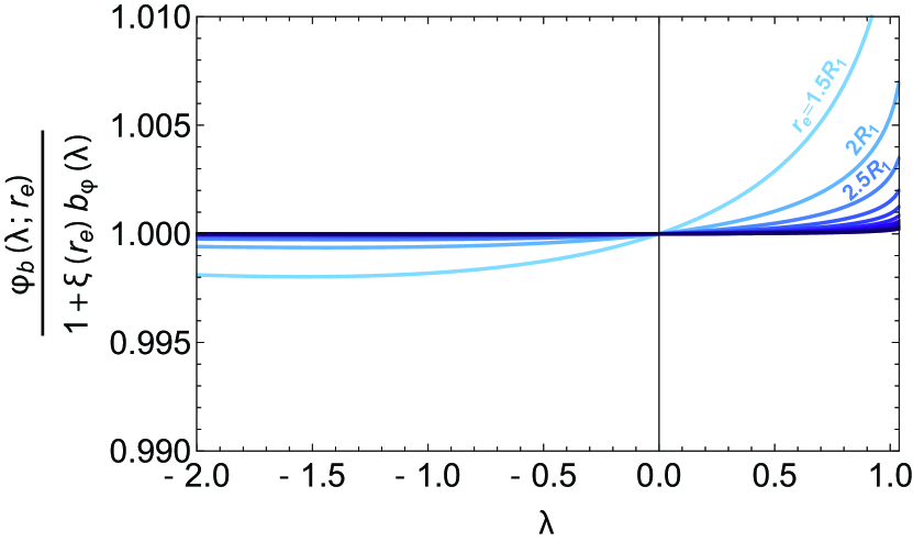
For n=1𝑛1n=1 cell, Fig. 3 shows the convergence of the approximation defined by equation (37) towards the exact value of φb(λ;re)subscript𝜑𝑏𝜆subscript𝑟𝑒\varphi_{b}(\lambda;r_{e}) computed from equations (18), (27) and (28) as the distance resubscript𝑟𝑒r_{e} increases. The convergence is fast, reaching sub-percent precision even for relatively small separations re>2R1superscriptsimilar-tosubscript𝑟𝑒2subscript𝑅1r_{e}\lower 2.15277pt\hbox{$\;\buildrel>\over{\sim}\;$}2R_{1}. As expected, the agreement is best for small values of λ𝜆\lambda, while deviations appear in the tails. Those conclusions are expected to hold similarly for a higher number n𝑛n of cells.

Refer to caption
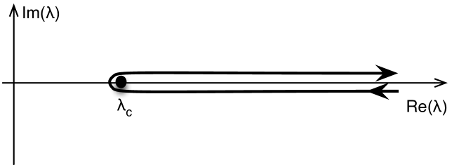
Figure 3: Ratio between φb(λ;re)subscript𝜑𝑏𝜆subscript𝑟𝑒\varphi_{b}(\lambda;r_{e}), the exact generating function of cumulants of the form ρ1pρ(re)csubscriptdelimited-⟨⟩superscriptsubscript𝜌1𝑝𝜌subscript𝑟𝑒𝑐\langle\rho_{1}^{p}\rho(r_{e})\rangle_{c} and its large-distance approximation φb(λ;re)=1+ξ(re)bφ(λ)subscript𝜑𝑏𝜆subscript𝑟𝑒1𝜉subscript𝑟𝑒subscript𝑏𝜑𝜆\varphi_{b}(\lambda;r_{e})=1+\xi(r_{e})b_{\varphi}(\lambda) for a power-law density power spectrum with index ns=1.6subscript𝑛𝑠1.6n_{s}=-1.6 and variance σ2=0.3superscript𝜎20.3\sigma^{2}=0.3. The separation resubscript𝑟𝑒r_{e} spans the range between re=3/2R1subscript𝑟𝑒32subscript𝑅1r_{e}=3/2R_{1} (light blue) and re=6R1subscript𝑟𝑒6subscript𝑅1r_{e}=6R_{1} (dark blue) as labelled. Note that the critical point in this case is λc1.05subscript𝜆𝑐1.05\lambda_{c}\approx 1.05.

4.2 The n+m formalism at large separation

Let us finally focus on the n+m𝑛𝑚n+m formalism where n𝑛n concentric cells at a distance resubscript𝑟𝑒r_{e} from m𝑚m other concentric cells are considered. The rest of the paper is devoted to the study of this configuration, illustrated in the right-hand panel of Fig. 2, in order to investigate the large-separation two-point statistics of densities in concentric cells.

In this large-separation limit, we can write down (see appendix B) the joint cumulants for two sets, separated by resubscript𝑟𝑒r_{e} much larger than Risubscript𝑅𝑖R_{i}, at leading order in terms of the two-point cumulants containing one power of the density in one location and any powers of the density in the second location (and generated by φbsubscript𝜑𝑏\varphi_{b}, see Section 3.2)

ρ1p1ρnpnρ1q1ρmqmc=\displaystyle\langle\rho_{1}^{p_{1}}\dots\rho_{n}^{p_{n}}{\rho^{\prime}}_{1}^{q_{1}}\dots\rho^{\prime}_{m}{}^{q_{m}}\rangle_{c}=
1ξ(re)ρ1p1ρnpnρicρiρ1q1ρmqmc,\displaystyle\hskip 28.45274pt\frac{1}{\xi(r_{e})}\langle\rho_{1}^{p_{1}}\dots\rho_{n}^{p_{n}}{\rho^{\prime}}_{i}\rangle_{c}\langle\rho_{i}{\rho^{\prime}}_{1}^{q_{1}}\dots\rho^{\prime}_{m}{}^{q_{m}}\rangle_{c}\,, (38)

where the {ρk=ρ1,k}ksubscriptsubscript𝜌𝑘subscript𝜌1𝑘𝑘\{\rho_{k}=\rho_{1,k}\}_{k} correspond to a set of radii {Rk}ksubscriptsubscript𝑅𝑘𝑘\{R_{k}\}_{k} of cells centred at, say, the origin, the {ρk=ρ2,k}ksubscriptsubscriptsuperscript𝜌𝑘subscript𝜌2𝑘𝑘\{\rho^{\prime}_{k}=\rho_{2,k}\}_{k} correspond to a set of radii {Rk}ksubscriptsubscriptsuperscript𝑅𝑘𝑘\{R^{\prime}_{k}\}_{k} of cells centred on a point at distance resubscript𝑟𝑒r_{e} from the origin and pisubscript𝑝𝑖p_{i} and qisubscript𝑞𝑖q_{i} are non-zero. Equation (38) can be easily understood from a diagrammatic point of view. Indeed, in the large-separation regime, the dominant contribution will come from the configuration in which there is only one leg linking two connected diagrams belonging to each location (see also Bernardeau (1996) for details).

At the level of the generating functions, equations (37) and (38) imply that

φ({λk},{λk};re)=𝜑subscript𝜆𝑘subscriptsuperscript𝜆𝑘subscript𝑟𝑒absent\displaystyle\varphi(\{\lambda_{k}\},\{\lambda^{\prime}_{k}\};r_{e})=
φ({λk})+φ({λk})+ξ(re)bφ({λk})bφ({λk}),𝜑subscript𝜆𝑘𝜑subscriptsuperscript𝜆𝑘𝜉subscript𝑟𝑒subscript𝑏𝜑subscript𝜆𝑘subscript𝑏𝜑subscriptsuperscript𝜆𝑘\displaystyle\hskip 11.38092pt\varphi(\{\lambda_{k}\}){+}\varphi(\{\lambda^{\prime}_{k}\})+\xi(r_{e})\,b_{\varphi}(\{\lambda_{k}\})\,b_{\varphi}(\{\lambda^{\prime}_{k}\})\,, (39)

where φ({λk},{λk};re)𝜑subscript𝜆𝑘subscriptsuperscript𝜆𝑘subscript𝑟𝑒\varphi(\{\lambda_{k}\},\{\lambda^{\prime}_{k}\};r_{e}) is the generating functions of the joint cumulants ρ1p1ρnpnρ1q1ρmqmc\langle\rho_{1}^{p_{1}}\dots\rho_{n}^{p_{n}}{\rho^{\prime}}_{1}^{q_{1}}\dots\rho^{\prime}_{m}{}^{q_{m}}\rangle_{c}. Equation (39) is the cornerstone of this paper.

4.3 Consequences for the joint PDFs

The structure of equation (39) for the cumulant generating function has direct consequences at the level of the corresponding joint PDF. Let us consider again two sets of concentric cells separated by a distance resubscript𝑟𝑒r_{e}, and define the corresponding densities {ρ^k}{ρ^1,k}subscript^𝜌𝑘subscript^𝜌1𝑘\{{\hat{\rho}}_{k}\}\equiv\{{\hat{\rho}}_{1,k}\} and {ρ^k}{ρ^2,k}subscriptsuperscript^𝜌𝑘subscript^𝜌2𝑘\{{\hat{\rho}}^{\prime}_{k}\}\equiv\{{\hat{\rho}}_{2,k}\}. For large separations, the joint PDF 𝒫({ρ^k},{ρ^k};re)𝒫subscript^𝜌𝑘subscriptsuperscript^𝜌𝑘subscript𝑟𝑒{\cal P}(\{{\hat{\rho}}_{k}\},\{{\hat{\rho}}^{\prime}_{k}\};r_{e}) takes, at leading order, the following form

𝒫({ρ^k},{ρ^k};re)=𝒫({ρ^k})𝒫({ρ^k})[1+ξ(re)b({ρ^k})b({ρ^k})],𝒫subscript^𝜌𝑘subscriptsuperscript^𝜌𝑘subscript𝑟𝑒𝒫subscript^𝜌𝑘𝒫subscriptsuperscript^𝜌𝑘delimited-[]1𝜉subscript𝑟𝑒𝑏subscript^𝜌𝑘𝑏subscriptsuperscript^𝜌𝑘{\cal P}(\{{\hat{\rho}}_{k}\},\{{{\hat{\rho}}^{\prime}}_{k}\};r_{e})=\\ {\cal P}(\{{\hat{\rho}}_{k}\}){\cal P}(\{{{\hat{\rho}}^{\prime}}_{k}\})\left[1+\xi(r_{e})b(\{{\hat{\rho}}_{k}\})b(\{{{\hat{\rho}}^{\prime}}_{k}\})\right]\,, (40)

given that

𝒫({ρ^k})=dλ12πidλn2πiexp(λiρ^i+φ({λk})),𝒫subscript^𝜌𝑘dsubscript𝜆12𝜋idsubscript𝜆𝑛2𝜋isubscript𝜆𝑖subscript^𝜌𝑖𝜑subscript𝜆𝑘{\cal P}(\{{\hat{\rho}}_{k}\})=\int\frac{\hbox{d}\lambda_{1}}{2\pi\hbox{i}}\dots\frac{\hbox{d}\lambda_{n}}{2\pi\hbox{i}}\exp\left({-}\lambda_{i}{\hat{\rho}}_{i}{+}\varphi(\{\lambda_{k}\})\right)\,, (41)

and

b({ρ^k})𝒫({ρ^k})=dλ12πidλn2πibφ({λk})exp(λiρ^i+φ({λk})),𝑏subscript^𝜌𝑘𝒫subscript^𝜌𝑘dsubscript𝜆12𝜋idsubscript𝜆𝑛2𝜋isubscript𝑏𝜑subscript𝜆𝑘subscript𝜆𝑖subscript^𝜌𝑖𝜑subscript𝜆𝑘b(\{{\hat{\rho}}_{k}\})\,{\cal P}(\{{\hat{\rho}}_{k}\})=\\ \int\frac{\hbox{d}\lambda_{1}}{2\pi\hbox{i}}\dots\frac{\hbox{d}\lambda_{n}}{2\pi\hbox{i}}b_{\varphi}(\{\lambda_{k}\})\exp\left({-}\lambda_{i}{\hat{\rho}}_{i}{+}\varphi(\{\lambda_{k}\})\right), (42)

where the bias cumulant generating function bφ({λk})subscript𝑏𝜑subscript𝜆𝑘b_{\varphi}(\{\lambda_{k}\}) is given by equation (36) and we have introduced the corresponding effective bias function, b({ρ^k})𝑏subscript^𝜌𝑘b(\{{\hat{\rho}}_{k}\}) (that will also simply be called “bias” or “bias function” in what follows). Note that measured densities will henceforth be denoted with a hat in order to avoid confusion with variables intervening in the computation of the cumulant generating functions (see for instance equation (19)).

Equation (42) is one of the main results of this paper. It defines the bias functions we introduced in equation (5), which is dual to equation (36) in the duality defined by PDF versus generating functions. Correspondingly, equation (40) is dual to equation (39). It is easy to show that the bias functions, b({ρ^k})𝑏subscript^𝜌𝑘b(\{{\hat{\rho}}_{k}\}), have an analytical asymptote at low density which can be derived using a steepest descent method in equations (41) and (42)

b({ρ^k})bφ({λk=kΨ({ρ^i})}),𝑏subscript^𝜌𝑘subscript𝑏𝜑subscript𝜆𝑘subscript𝑘Ψsubscript^𝜌𝑖b(\{{\hat{\rho}}_{k}\})\approx b_{\varphi}(\{\lambda_{k}=\partial_{k}\Psi(\{{\hat{\rho}}_{i}\})\})\,, (43)

where kΨ=Ψ/ρksubscript𝑘ΨΨsubscript𝜌𝑘\partial_{k}\Psi=\partial\Psi/\partial\rho_{k}. In practice, we will make use below of the following low-density approximation

b({ρ^k})i=1nj=1nΞij({Rkρ^k1/3})ζ1(ρ^j),𝑏subscript^𝜌𝑘superscriptsubscript𝑖1𝑛superscriptsubscript𝑗1𝑛subscriptΞ𝑖𝑗subscript𝑅𝑘superscriptsubscript^𝜌𝑘13superscript𝜁1subscript^𝜌𝑗b(\{{\hat{\rho}}_{k}\})\approx\sum_{i=1}^{n}\sum_{j=1}^{n}\Xi_{ij}(\{R_{k}{\hat{\rho}}_{k}^{1/3}\})\zeta^{-1}({\hat{\rho}}_{j})\,, (44)

which allows to go beyond the critical point where λi=iΨ({ρ^k})subscript𝜆𝑖subscript𝑖Ψsubscript^𝜌𝑘\lambda_{i}=\partial_{i}\Psi(\{{\hat{\rho}}_{k}\}) is ill-defined.

4.4 Properties of the density bias

From equation (36), one can show that bφ=0subscript𝑏𝜑0b_{\varphi}=0 and bφ(0)=1superscriptsubscript𝑏𝜑01b_{\varphi}^{\prime}(0)=1. Using equation (42), it follows that the bias functions obey the following two relations

0dρ^k𝒫({ρ^k})b({ρ^k})=0,superscriptsubscript0dsubscript^𝜌𝑘𝒫subscript^𝜌𝑘𝑏subscript^𝜌𝑘0\displaystyle\int_{0}^{\infty}\hbox{d}{\hat{\rho}}_{k}{\cal P}(\{{\hat{\rho}}_{k}\})\,b(\{{\hat{\rho}}_{k}\})=0\,, (45)
0dρ^k𝒫({ρ^k})b({ρ^k})ρ^k=1.superscriptsubscript0dsubscript^𝜌𝑘𝒫subscript^𝜌𝑘𝑏subscript^𝜌𝑘subscript^𝜌𝑘1\displaystyle\int_{0}^{\infty}\hbox{d}{\hat{\rho}}_{k}{\cal P}(\{{\hat{\rho}}_{k}\})\,b(\{{\hat{\rho}}_{k}\}){\hat{\rho}}_{k}=1\,. (46)

These properties ensure the normalisation of the PDF and the definition of ξ𝜉\xi, the dark matter correlation function.

In particular, we will make use of these identities to measure the density bias function either using the auto-correlation of cells of a given density

1+b2(ρ^)ξ(re)=0dρ^kdρ^k𝒫({ρ^k},{ρ^k};re)δD(ρ^kρ^)δD(ρ^kρ^)0dρ^kdρ^k𝒫({ρ^k})𝒫({ρ^k})δD(ρ^kρ^)δD(ρ^kρ^),1superscript𝑏2^𝜌𝜉subscript𝑟𝑒superscriptsubscript0dsubscript^𝜌𝑘dsubscriptsuperscript^𝜌𝑘𝒫subscript^𝜌𝑘subscriptsuperscript^𝜌𝑘subscript𝑟𝑒subscript𝛿Dsubscript^𝜌𝑘^𝜌subscript𝛿Dsubscriptsuperscript^𝜌𝑘^𝜌superscriptsubscript0dsubscript^𝜌𝑘dsubscriptsuperscript^𝜌𝑘𝒫subscript^𝜌𝑘𝒫subscriptsuperscript^𝜌𝑘subscript𝛿Dsubscript^𝜌𝑘^𝜌subscript𝛿Dsubscriptsuperscript^𝜌𝑘^𝜌1+b^{2}({\hat{\rho}})\xi(r_{e})=\\ \frac{\displaystyle\int_{0}^{\infty}\hbox{d}{\hat{\rho}}_{k}\hbox{d}{\hat{\rho}}^{\prime}_{k}{\cal P}(\{{\hat{\rho}}_{k}\},\{{{\hat{\rho}}^{\prime}}_{k}\};r_{e})\delta_{\text{D}}({\hat{\rho}}_{k}-{\hat{\rho}})\delta_{\text{D}}({\hat{\rho}}^{\prime}_{k}-{\hat{\rho}})}{\displaystyle\int_{0}^{\infty}\hbox{d}{\hat{\rho}}_{k}\hbox{d}{\hat{\rho}}^{\prime}_{k}{\cal P}(\{{\hat{\rho}}_{k}\}){\cal P}(\{{\hat{\rho}}^{\prime}_{k}\})\delta_{\text{D}}({\hat{\rho}}_{k}-{\hat{\rho}})\delta_{\text{D}}({\hat{\rho}}^{\prime}_{k}-{\hat{\rho}})}\,, (47)

or their cross-correlations

1+b(ρ^)ξ(re)=0dρ^kdρ^k𝒫({ρ^k},{ρ^k};re)δD(ρ^kρ^)ρ^k0dρ^k𝒫({ρ^k})δD(ρ^kρ^).1𝑏^𝜌𝜉subscript𝑟𝑒superscriptsubscript0dsubscript^𝜌𝑘dsubscriptsuperscript^𝜌𝑘𝒫subscript^𝜌𝑘subscriptsuperscript^𝜌𝑘subscript𝑟𝑒subscript𝛿Dsubscript^𝜌𝑘^𝜌subscriptsuperscript^𝜌𝑘superscriptsubscript0dsubscript^𝜌𝑘𝒫subscript^𝜌𝑘subscript𝛿Dsubscript^𝜌𝑘^𝜌1+b({\hat{\rho}})\xi(r_{e})=\\ \frac{\displaystyle\int_{0}^{\infty}\hbox{d}{\hat{\rho}}_{k}\hbox{d}{\hat{\rho}}^{\prime}_{k}{\cal P}(\{{\hat{\rho}}_{k}\},\{{{\hat{\rho}}^{\prime}}_{k}\};r_{e})\delta_{\text{D}}({\hat{\rho}}_{k}-{\hat{\rho}}){\hat{\rho}}^{\prime}_{k}}{\displaystyle\int_{0}^{\infty}\hbox{d}{\hat{\rho}}_{k}{\cal P}(\{{\hat{\rho}}_{k}\})\delta_{\text{D}}({\hat{\rho}}_{k}-{\hat{\rho}})}\,. (48)

In practice, measurements will be done in bins of a given width, meaning that Dirac delta functions will be replaced by stepwise functions (see Section 6.1 below).

4.5 Slope bias

In the two-cell case, instead of (ρ^1,ρ^2)subscript^𝜌1subscript^𝜌2({\hat{\rho}}_{1},{\hat{\rho}}_{2}), we will use the variables (ρ^,s^)^𝜌^𝑠({\hat{\rho}},\hat{s}) describing the inner density ρ^=ρ^1^𝜌subscript^𝜌1{\hat{\rho}}={\hat{\rho}}_{1} and slope s^=(ρ^2ρ^1)R1/ΔR^𝑠subscript^𝜌2subscript^𝜌1subscript𝑅1Δ𝑅\hat{s}=({\hat{\rho}}_{2}-{\hat{\rho}}_{1})R_{1}/\Delta R with ΔR=R2R1Δ𝑅subscript𝑅2subscript𝑅1\Delta R=R_{2}-R_{1}. The slope bias, b(s^)𝑏^𝑠b(\hat{s}), will be investigated using the relation

1+b(s^)ξ(re)=0dρ^ds^𝒫({ρ^},{s^};re)δD(s^s^)ρ^ds^𝒫(s^)δD(s^s^).1𝑏^𝑠𝜉subscript𝑟𝑒superscriptsubscript0d^𝜌superscriptsubscriptdsuperscript^𝑠𝒫^𝜌superscript^𝑠subscript𝑟𝑒subscript𝛿Dsuperscript^𝑠^𝑠^𝜌superscriptsubscriptdsuperscript^𝑠𝒫superscript^𝑠subscript𝛿Dsuperscript^𝑠^𝑠1+b({\hat{s}})\xi(r_{e})=\frac{\displaystyle\int_{0}^{\infty}\!\!\!\!\!\hbox{d}{\hat{\rho}}\int_{-\infty}^{\infty}\!\!\!\!\!\hbox{d}{\hat{s}}^{\prime}\,{\cal P}(\{{\hat{\rho}}\},\{{\hat{s}}^{\prime}\};r_{e})\delta_{\text{D}}({\hat{s}}^{\prime}-{\hat{s}}){\hat{\rho}}}{\displaystyle\int_{-\infty}^{\infty}\!\!\!\!\!\hbox{d}{\hat{s}}^{\prime}\,{\cal P}({\hat{s}}^{\prime})\delta_{\text{D}}({\hat{s}}^{\prime}-{\hat{s}})}\,. (49)

In equation (49), 𝒫({ρ^},{s^};re)𝒫^𝜌superscript^𝑠subscript𝑟𝑒{\cal P}(\{{\hat{\rho}}\},\{{\hat{s}}^{\prime}\};r_{e}) is a marginal of the two-cell PDF given by 𝒫({ρ^1,s^1},{ρ^2,s^2};re)δD(ρ^1ρ^)δD(s^2s^)𝒫subscript^𝜌1subscript^𝑠1subscript^𝜌2subscript^𝑠2subscript𝑟𝑒subscript𝛿Dsubscript^𝜌1^𝜌subscript𝛿Dsubscript^𝑠2superscript^𝑠{\cal P}(\{{\hat{\rho}}_{1},{\hat{s}}_{1}\},\{{\hat{\rho}}_{2},{\hat{s}}_{2}\};r_{e})\delta_{\rm D}({\hat{\rho}}_{1}-{\hat{\rho}})\delta_{\rm D}({\hat{s}}_{2}-{\hat{s}}^{\prime}) integrated over ρ^1subscript^𝜌1{\hat{\rho}}_{1}, s^1subscript^𝑠1{\hat{s}}_{1}, ρ^2subscript^𝜌2{\hat{\rho}}_{2} and s^2subscript^𝑠2{\hat{s}}_{2}. The slope bias, b(s^)𝑏^𝑠b({\hat{s}}), is defined as the Inverse Laplace transform of the slope bias cumulant generating function

bs(μ)bφ(R1ΔRμ,R1ΔRμ),subscript𝑏𝑠𝜇subscript𝑏𝜑subscript𝑅1Δ𝑅𝜇subscript𝑅1Δ𝑅𝜇b_{s}(\mu)\equiv b_{\varphi}\left(-\frac{R_{1}}{\Delta R}\mu,\frac{R_{1}}{\Delta R}\mu\right)\,, (50)

via

b(s^)𝒫(s^)=dμ2πibs(μ)exp(μs^+φs(μ)),𝑏^𝑠𝒫^𝑠d𝜇2𝜋isubscript𝑏𝑠𝜇𝜇^𝑠subscript𝜑𝑠𝜇b(\hat{s})\,{\cal P}(\hat{s})=\int\frac{\hbox{d}\mu}{2\pi\hbox{i}}b_{s}(\mu)\exp\left({-}\mu\hat{s}{+}\varphi_{s}(\mu)\right)\,, (51)

with the slope PDF defined as

𝒫(s^)=dμ2πiexp(μs^+φs(μ)).𝒫^𝑠d𝜇2𝜋i𝜇^𝑠subscript𝜑𝑠𝜇{\cal P}(\hat{s})=\int\frac{\hbox{d}\mu}{2\pi\hbox{i}}\exp\left({-}\mu\hat{s}{+}\varphi_{s}(\mu)\right)\,. (52)

Equations (51) and (50) follow from the rewriting

λ1ρ1+λ2ρ2subscript𝜆1subscript𝜌1subscript𝜆2subscript𝜌2\displaystyle\lambda_{1}\rho_{1}+\lambda_{2}\rho_{2} =(λ1+λ2)ρ1+ΔRR1λ2s,absentsubscript𝜆1subscript𝜆2subscript𝜌1Δ𝑅subscript𝑅1subscript𝜆2𝑠\displaystyle=(\lambda_{1}+\lambda_{2})\rho_{1}+\frac{\Delta R}{R_{1}}\lambda_{2}s\,, (53)
=λρ+μs,absent𝜆𝜌𝜇𝑠\displaystyle=\lambda\rho+\mu s\,, (54)

which makes explicit the relation between (λ1,λ2)subscript𝜆1subscript𝜆2(\lambda_{1},\lambda_{2}) and (λ,μ)𝜆𝜇(\lambda,\mu) and consequently the relation between the slope cumulant generating function, φssubscript𝜑𝑠\varphi_{s}, and φ𝜑\varphi

φs(μ)=φ(λ1=R1ΔRμ,λ2=R1ΔRμ).subscript𝜑𝑠𝜇𝜑formulae-sequencesubscript𝜆1subscript𝑅1Δ𝑅𝜇subscript𝜆2subscript𝑅1Δ𝑅𝜇\varphi_{s}(\mu)=\varphi\left(\lambda_{1}=-\frac{R_{1}}{\Delta R}\mu,\lambda_{2}=\frac{R_{1}}{\Delta R}\mu\right)\,. (55)

Imposing λ=0𝜆0\lambda=0 therefore allows us to marginalise over ρ𝜌\rho and get the slope bias.

It has to be noted that the slope bias obeys similar contraints as the density bias namely

ds^𝒫(s^)b(s^)=0,superscriptsubscriptd^𝑠𝒫^𝑠𝑏^𝑠0\displaystyle\int_{-\infty}^{\infty}\hbox{d}{\hat{s}}\,{\cal P}({\hat{s}})\,b({\hat{s}})=0\,, (56)
ds^𝒫(s^)b(s^)s^=0.superscriptsubscriptd^𝑠𝒫^𝑠𝑏^𝑠^𝑠0\displaystyle\int_{-\infty}^{\infty}\hbox{d}{\hat{s}}\,{\cal P}({\hat{s}})\,b({\hat{s}}){\hat{s}}=0\,. (57)

5 Implementation for realistic Pksubscript𝑃𝑘P_{k}

Refer to caption
Refer to caption
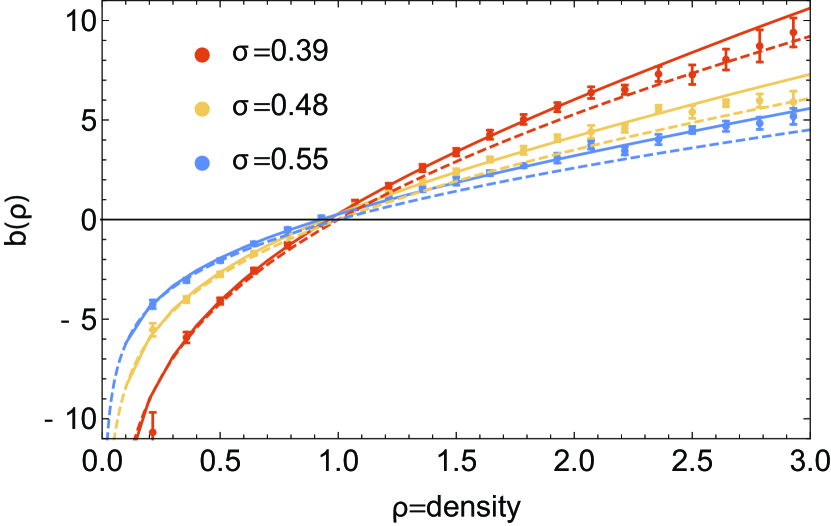
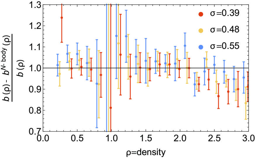
Figure 4: Left-hand panel: The density bias function b(ρ^)𝑏^𝜌b({\hat{\rho}}) for different values of the variance (σ𝜎\sigma=0.39, 0.48 and 0.55 for respectively the red, yellow and blue lines). The prediction computed numerically via equation (42) is displayed with solid lines while the dashed lines correspond to the analytical low-density approximations given by equation (44). Measurements in the simulation for spheres of radius R=10𝑅10R=10Mpc/habsent/h separated by re=20subscript𝑟𝑒20r_{e}=20Mpc/habsent/h are shown with error bars and are successfully compared to the numerical prediction (solid lines) for the full range of variances and densities. The low-density approximations break down for ρ>1superscriptsimilar-to𝜌1\rho\lower 2.15277pt\hbox{$\;\buildrel>\over{\sim}\;$}1. Right-hand panel: Residuals between the measured density bias (error bars) and its numerical prediction from equation (42) (displayed with solid lines on the left-hand panel). The yellow and red error bars have been shifted along the x-axis respectively by 0.03 and 0.06 for aesthetic purposes.

In order to explicitly compute the bias functions for a realistic (ΛΛ\LambdaCDM) power spectrum, Plin(k)superscript𝑃lin𝑘P^{{\rm lin}}(k), and compare those predictions to simulations, we follow BPC and approximate the variance

σ2(R,R)=d3k(2π)3Plin(k)W3D2(kR),superscript𝜎2𝑅𝑅superscriptd3ksuperscript2𝜋3superscript𝑃lin𝑘subscriptsuperscript𝑊23D𝑘𝑅\sigma^{2}(R,R)=\int\frac{\hbox{d}^{3}\textbf{k}}{(2\pi)^{3}}P^{{\rm lin}}(k)W^{2}_{\rm 3D}(kR)\,, (58)

using an analytical formula describing the scale-dependencies

σ2(R,R)=2σ2(Rp,Rp)(R/Rp)n1+3+(R/Rp)n2+3,superscript𝜎2𝑅𝑅2superscript𝜎2subscript𝑅𝑝subscript𝑅𝑝superscript𝑅subscript𝑅𝑝subscript𝑛13superscript𝑅subscript𝑅𝑝subscript𝑛23\sigma^{2}(R,R)=\frac{2\sigma^{2}(R_{p},R_{p})}{(R/R_{p})^{n_{1}+3}+(R/R_{p})^{n_{2}+3}}\,, (59)

where n1subscript𝑛1n_{1} and n2subscript𝑛2n_{2} are chosen to reproduce the linear theory index n(R)=3dlog(σ2(R,R))/dlogR𝑛𝑅3dsuperscript𝜎2𝑅𝑅d𝑅n(R)=-3-{\hbox{d}\log(\sigma^{2}(R,R))}/{\hbox{d}\log R} and running, α(R)=dlog(n(R))/dlogR𝛼𝑅d𝑛𝑅d𝑅\alpha(R)={\hbox{d}\log(n(R))}/{\hbox{d}\log R} at the pivot scale Rpsubscript𝑅𝑝R_{p}. Note that in fine the amplitude, σ0=σ(Rp,Rp)subscript𝜎0𝜎subscript𝑅𝑝subscript𝑅𝑝\sigma_{0}=\sigma(R_{p},R_{p}), can be simply measured and not necessarily predicted by linear theory as it can be easily scaled out using the relation

φσ0({λk})=1σ02φ1({λk/σ02}),subscript𝜑subscript𝜎0subscript𝜆𝑘1superscriptsubscript𝜎02subscript𝜑1subscript𝜆𝑘superscriptsubscript𝜎02\varphi_{\sigma_{0}}(\{\lambda_{k}\})=\frac{1}{\sigma_{0}^{2}}\varphi_{1}(\{\lambda_{k}/\sigma_{0}^{2}\}), (60)

while the variable ρksubscript𝜌𝑘\rho_{k} are independent of σ0subscript𝜎0\sigma_{0}. In practice, we take here (n1+n2)/2=1.58subscript𝑛1subscript𝑛221.58(n_{1}+n_{2})/2=-1.58 and n1n2=1.23subscript𝑛1subscript𝑛21.23n_{1}-n_{2}=1.23 at Rp=10subscript𝑅𝑝10R_{p}=10Mpc/habsent/h and σ2(Rp,Rp)superscript𝜎2subscript𝑅𝑝subscript𝑅𝑝\sigma^{2}(R_{p},R_{p}) is measured at different redshifts in the simulation.

Using the parametrization (59) of σ(R,R)𝜎𝑅𝑅\sigma(R,R), we can then analytically predict the one-cell rate function ΨΨ\Psi, the cumulant generating function φ𝜑\varphi and the bias function bφsubscript𝑏𝜑b_{\varphi} and finally numerically compute the PDF 𝒫(ρ^)𝒫^𝜌\cal P({\hat{\rho}}) and bias function b(ρ^)𝑏^𝜌b({\hat{\rho}}). In this paper, the numerical integrations are done, in the one-cell case, using a path parallel to the imaginary axis λ=λ0+Δλi𝜆subscript𝜆0Δ𝜆i\lambda=\lambda_{0}+\Delta\lambda\,\hbox{i} where λ0=Ψ(min(ρ^,ρc))subscript𝜆0superscriptΨmin^𝜌subscript𝜌𝑐\lambda_{0}={\Psi^{\prime}}(\textrm{min}({\hat{\rho}},\rho_{c})), i𝑖i goes from 1 to the number of points nstepssubscript𝑛stepsn_{\rm steps} which is set to 1000 and the step, ΔλΔ𝜆\Delta\lambda, depends on the value of the density ρ^^𝜌\hat{\rho} (typically larger for smaller densities).

The resulting prediction for the density bias is shown in the left-hand panel of Fig. 4 (solid lines). As expected from previous studies, this figure shows that the bias is zero only in regions where the density is around the mean i.e ρ1𝜌1\rho\approx 1. This can easily be understood as 𝒫({ρ^},{ρ^=1};re)/𝒫(1)=𝒫(ρ^)𝒫^𝜌superscript^𝜌1subscript𝑟𝑒𝒫1𝒫^𝜌{\cal P}(\{{\hat{\rho}}\},\{{\hat{\rho}}^{\prime}=1\};r_{e})/{\cal P}(1)={\cal P}({\hat{\rho}}) if resubscript𝑟𝑒r_{e} is large enough. Overdense regions are then positively biased while underdense regions are less clustered (negatively biased). This is also consistent with Kaiser (1984) as the left-hand panel of Fig. 4 shows that the larger the density, the stronger the bias. Note that unlike the Gaussian peak bias which scales like the contrast for large densities, here the scaling of the non-linear bias departs from linearity with typically bρ0.8proportional-to𝑏superscript𝜌0.8b\propto\rho^{0.8} for large densities but is recovered in the very large density limit ρ^>10superscriptsimilar-to^𝜌10{\hat{\rho}}\lower 2.15277pt\hbox{$\;\buildrel>\over{\sim}\;$}10. Indeed, it is found (see Appendix E for more details) that the asymptotic behaviour of the bias function is given by

b(ρ^)ρ^(ρ^ρc)(λcρc(ρc1/ν11/ν)+1νφc)ν(ρc1/ν1)2ρc11/ν^𝜌absent𝑏^𝜌^𝜌subscript𝜌𝑐subscript𝜆𝑐subscript𝜌𝑐superscriptsubscript𝜌𝑐1𝜈11𝜈1𝜈subscript𝜑𝑐𝜈superscriptsuperscriptsubscript𝜌𝑐1𝜈12superscriptsubscript𝜌𝑐11𝜈b({\hat{\rho}})\xrightarrow[{\hat{\rho}}\rightarrow\infty]{}\frac{({\hat{\rho}}-\rho_{c})(\lambda_{c}\rho_{c}(\rho_{c}^{1/\nu}-1-1/\nu)+\frac{1}{\nu}\varphi_{c})}{\nu(\rho_{c}^{1/\nu}-1)^{2}\rho_{c}^{1-1/\nu}} (61)

when the integral is dominated by the singular point in equations (41) and (42). It has to be noted that this asymptotic behaviour depends on the existence of the singular point, ρcsubscript𝜌𝑐\rho_{c}, which is due to the application of a large-deviation principle to the density field. However, as shown in Uhlemann et al. (2015), this singular point can be removed by applying a large-deviation principle to a non-linear transformation of the density field, for instance its logarithm. In that case, we expect the asymptotic behaviour to be slightly modified as shown in that paper.

Note also that the bias of large-density regions is reduced for larger variances. This trend persists even if the density bias is plotted against the contrast νc=(ρ^1)/σsubscript𝜈𝑐^𝜌1𝜎\nu_{c}=({\hat{\rho}}-1)/\sigma instead of ρ^^𝜌{\hat{\rho}}. The left-hand panel of Fig. 4 also displays the low-density approximation given by equation (44). This approximation is only valid in a limited range of densities typically for ρ^1less-than-or-similar-to^𝜌1{\hat{\rho}}\lesssim 1.

In the two-cell case, one need to compute the covariance matrix between initial densities in spheres of radii R1subscript𝑅1R_{1} and R2subscript𝑅2R_{2}

σ2(Ri,Rj)=d3k(2π)3Plin(k)W3D(kRi)W3D(kRj),superscript𝜎2subscript𝑅𝑖subscript𝑅𝑗superscriptd3ksuperscript2𝜋3superscript𝑃lin𝑘subscript𝑊3D𝑘subscript𝑅𝑖subscript𝑊3D𝑘subscript𝑅𝑗\sigma^{2}(R_{i},R_{j})=\int\frac{\hbox{d}^{3}\textbf{k}}{(2\pi)^{3}}P^{{\rm lin}}(k)W_{\rm 3D}(kR_{i})W_{\rm 3D}(kR_{j})\,, (62)

where W3Dsubscript𝑊3DW_{\rm 3D} is the top-hat filter function

W3D(k)=3k2(sin(k)/kcos(k)).subscript𝑊3D𝑘3superscript𝑘2𝑘𝑘𝑘W_{\rm 3D}(k)=\frac{3}{k^{2}}(\sin(k)/k-\cos(k))\,. (63)

Again, for the sake of simplicity, we choose to parametrize this covariance matrix by

σ2(Ri,Ri)superscript𝜎2subscript𝑅𝑖subscript𝑅𝑖\displaystyle\sigma^{2}(R_{i},R_{i}) =σ2(Rp)(RiRp)ns(Rp)3,absentsuperscript𝜎2subscript𝑅𝑝superscriptsubscript𝑅𝑖subscript𝑅𝑝subscript𝑛𝑠subscript𝑅𝑝3\displaystyle=\sigma^{2}(R_{p})\left(\frac{R_{i}}{R_{p}}\right)^{-n_{s}(R_{p})-3}\,, (64)
σ2(Ri,Rj>i)superscript𝜎2subscript𝑅𝑖subscript𝑅𝑗𝑖\displaystyle\sigma^{2}(R_{i},R_{j>i}) =σ2(Rp)Rpns(Rp)+3𝒢(Ri,Rj,ns(Rp)),absentsuperscript𝜎2subscript𝑅𝑝superscriptsubscript𝑅𝑝subscript𝑛𝑠subscript𝑅𝑝3𝒢subscript𝑅𝑖subscript𝑅𝑗subscript𝑛𝑠subscript𝑅𝑝\displaystyle=\sigma^{2}(R_{p})R_{p}^{n_{s}(R_{p})+3}{\cal G}(R_{i},R_{j},n_{s}(R_{p}))\,, (65)

where

𝒢(x,y,ns)𝒢𝑥𝑦subscript𝑛𝑠\displaystyle{\cal G}(x,y,n_{s}) =Rpns3d3kknsW3D(kx)W3D(ky)d3kknW3D(kRp)W3D(kRp)absentsuperscriptsubscript𝑅𝑝subscript𝑛𝑠3superscriptd3ksuperscript𝑘subscript𝑛𝑠subscript𝑊3D𝑘𝑥subscript𝑊3D𝑘𝑦superscriptd3ksuperscript𝑘𝑛subscript𝑊3D𝑘subscript𝑅𝑝subscript𝑊3D𝑘subscript𝑅𝑝\displaystyle=R_{p}^{-n_{s}-3}\frac{\int{\hbox{d}^{3}\textbf{k}\,}k^{n_{s}}W_{\rm 3D}(kx)W_{\rm 3D}(ky)}{\int{\hbox{d}^{3}\textbf{k}\,}k^{n}W_{\rm 3D}(kR_{p})W_{\rm 3D}(kR_{p})}
=(x+y)α(x2+y2αxy)(yx)α(x2+y2+αxy)2α(ns+1)x3y3,absentsuperscript𝑥𝑦𝛼superscript𝑥2superscript𝑦2𝛼𝑥𝑦superscript𝑦𝑥𝛼superscript𝑥2superscript𝑦2𝛼𝑥𝑦superscript2𝛼subscript𝑛𝑠1superscript𝑥3superscript𝑦3\displaystyle=\!\frac{(x\!+\!y)^{\alpha}\!\!\left(\!x^{2}\!+\!y^{2}\!-\!\alpha xy\right)\!-\!(y\!-\!x)^{\alpha}\!\!\left(\!x^{2}\!+\!y^{2}\!+\!\alpha xy\right)}{2^{\alpha}(n_{s}+1)x^{3}y^{3}},

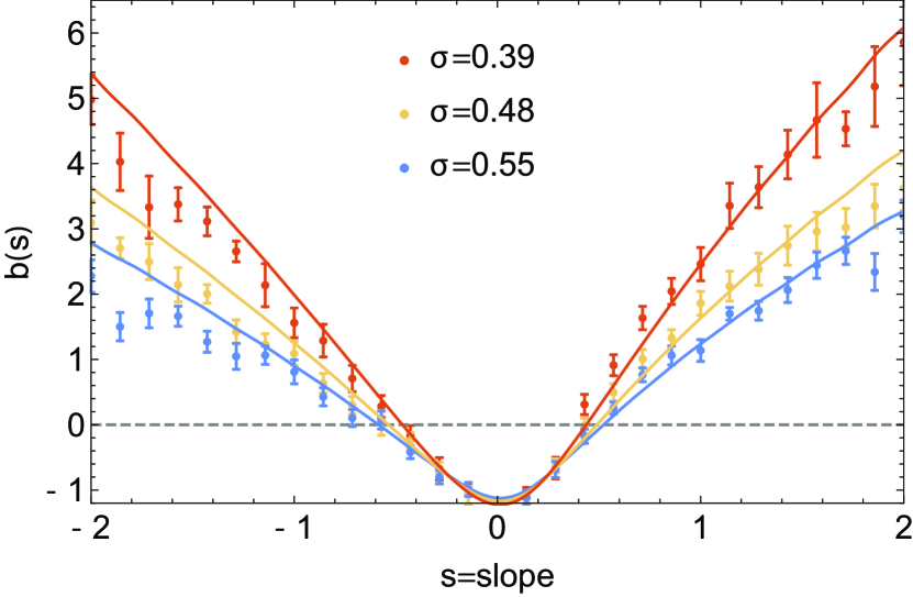
with α=1ns𝛼1subscript𝑛𝑠\alpha=1-n_{s}. We are now in a position to compute the two-cell rate function, cumulant generating function, PDF and finally the two-cell bias function. The slope bias b(s^)𝑏^𝑠b({\hat{s}}) predicted by this formalism is shown in Fig. 6 (right-hand panel). Two configurations are shown to be uncorrelated (b(s^)=0𝑏^𝑠0b({\hat{s}})=0) and roughly correspond to slopes s^±0.5^𝑠plus-or-minus0.5{\hat{s}}\approx\pm 0.5 with some σ𝜎\sigma-dependence. This situation is of particular interest as, according to equation (13), cosmic variance is drastically reduced in this case where only subdominant contributions will appear such as Poisson noise and small-scale effects. Besides this noteworthy case, it is found that small slopes (|s^|0.5less-than-or-similar-to^𝑠0.5|{\hat{s}}|\lesssim 0.5) are negatively biased while regions with larger (positive or negative) slope are more clustered. As expected, the bias is stronger for large slopes which typically correspond to sharp peaks (or voids) and will scale like b(s^)s^proportional-to𝑏^𝑠^𝑠b({\hat{s}})\propto{\hat{s}} in the very large slope limit as explained in appendix F. This asymptotic large |s|𝑠|s| behaviour can be compared once again to the linear Kaiser bias, given by equation (1), but in the contrast of the peak rather than the slope. Note also that the asymmetry of the bias function is weakened with variance.

The predictions for the density and slope bias functions are compared against simulations in the next section.

6 Validation against simulations

In the following we present the measurement of this bias function for the density ρ^^𝜌\hat{\rho} and for the density slope s^^𝑠{\hat{s}}.

The dark matter simulation (carried out with Gadget2, Springel, 2005) is characterized by the following ΛΛ\LambdaCDM cosmology: Ωm=0.265subscriptΩm0.265\Omega_{\rm m}=0.265, ΩΛ=0.735subscriptΩΛ0.735\Omega_{\Lambda}=0.735, n=0.958𝑛0.958n=0.958, H0=70subscript𝐻070H_{0}=70 kms1\cdot s^{-1}\cdotMpc-1 and σ8=0.8subscript𝜎80.8\sigma_{8}=0.8, Ωb=0.045subscriptΩ𝑏0.045\Omega_{b}=0.045 within one standard deviation of WMAP7 results (Komatsu et al., 2011). The box size is 500 Mpc/habsent/h sampled with 10243superscript102431024^{3} particles, the softening length 24 kpc/habsent/h. Initial conditions are generated using mpgrafic (Prunet et al., 2008). An Octree is built to count efficiently all particles within a given sequence of concentric spheres of radii between R=4,5𝑅45R=4,5\cdots up to 18Mpc/h18Mpc18{\rm Mpc}/h. The center of these spheres is sampled regularly on a grid of 10Mpc/h10Mpc10\,{\rm Mpc}/h aside, leading to 503=125,000superscript50312500050^{3}=125,000 estimates of the density per snapshot. Note that the cells overlap for radii larger than 5Mpc/h5Mpc5\,{\rm Mpc}/h.

6.1 Density bias function

The density bias is estimated from spheres of radius R=10Mpc/h𝑅10MpcR=10{\rm Mpc}/h that are separated by re=20subscript𝑟𝑒20r_{e}=20Mpc/habsent/h using the cross-correlations defined in equation (48). More precisely, we compute a sum over each sphere II\rm I with density ρIsubscript𝜌I\rho_{\rm I} and its 6 neighbours at distance re=20subscript𝑟𝑒20r_{e}=20Mpc/habsent/h labelled with the indices αI,jsubscript𝛼I𝑗\alpha_{{\rm I},j} for 1j61𝑗61\leq j\leq 6

b^(ρ^)=1ξ^[Ij=16(ρ^Δρ/2ρIρ^+Δρ/2)ραI,j6I(ρ^Δρ/2ρIρ^+Δρ/2)1]^𝑏^𝜌1^𝜉delimited-[]subscriptIsuperscriptsubscript𝑗16^𝜌Δ𝜌2subscript𝜌I^𝜌Δ𝜌2subscript𝜌subscript𝛼I𝑗6subscriptI^𝜌Δ𝜌2subscript𝜌I^𝜌Δ𝜌21\hat{b}({\hat{\rho}})=\frac{1}{\hat{\xi}}\!\left[\frac{\sum_{\rm I}\sum_{j=1}^{6}{\cal B}({\hat{\rho}}\!-\!\Delta\rho/2\leq\rho_{\rm I}\leq{\hat{\rho}}\!+\!\Delta\rho/2)\rho_{\alpha_{{\rm I},j}}}{6\sum_{\rm I}{\cal B}({\hat{\rho}}-\Delta\rho/2\leq\rho_{\rm I}\leq{\hat{\rho}}+\Delta\rho/2)}-1\right]

where {\cal B} is a boolean function which evaluates to one if the density is in a bin centred on ρ^^𝜌{\hat{\rho}} with width Δρ=3/21Δ𝜌321\Delta\rho=3/21 and the measured dark matter correlation function at distance resubscript𝑟𝑒r_{e} is given by

ξ^(re)=I=1Ntj=16ρIραI,j6Nt1.^𝜉subscript𝑟𝑒superscriptsubscriptI1subscriptNtsuperscriptsubscript𝑗16subscript𝜌Isubscript𝜌subscript𝛼I𝑗6subscriptNt1\hat{\xi}(r_{e})=\frac{\sum_{\rm I=1}^{\rm N_{t}}\sum_{j=1}^{6}\rho_{\rm I}\rho_{\alpha_{{\rm I},j}}}{6\mathrm{N_{t}}}-1. (66)

In practice, we count all pairs of spheres only once when computing ξ^(re)^𝜉subscript𝑟𝑒\hat{\xi}(r_{e}) by only considering three neighbours for each sphere. Error bars are then evaluated by computing the error on the mean of the density bias when the simulation is divided into eight sub-cubes.

The density bias b^(ρ^)^𝑏^𝜌\hat{b}({\hat{\rho}}) measured for different values of the variance is shown in the left-hand panel of Fig. 4 and successfully compared to the predictions obtained in Section 5. In particular and as expected, it is found that the bias is null for densities of 111. For count-in-cells, this trivially implies that imposing that the density equals its mean value within some sphere does not impact its neighbourhood sufficiently far enough. The right-hand panel of Fig. 4 displays the corresponding residuals and confirms the extremely good agreement between theory and measurements. Note that errors are relatively large for ρ^1^𝜌1{\hat{\rho}}\approx 1 as b(ρ^)𝑏^𝜌b({\hat{\rho}}) is very close to zero in this region. Note also that the apparent discrepancy between theory and prediction for the lower density bin at σ=0.39𝜎0.39\sigma=0.39 is mainly due to the fact that we did not take into account the size of the bin when predicting the density bias from equation (42) while it would have been necessary especially in such steep regions of the plot. Eventually, we conclude that the prediction is within the error bars of the simulations for the whole range of densities probed by our simulation meaning that a 10% accuracy at worst can be achieved with large-deviation theory. It is striking to see that the accuracy is poorer at higher redshift which could indicate that the main source of uncertainty here is not due to the theoretical prediction but to some numerical artefacts of our simulation. The (analytical) low-density approximation is shown to give a reasonable fit from 10%absentpercent10\approx 10\% precision for ρ1less-than-or-similar-to𝜌1\rho\lesssim 1 to order one for larger densities.

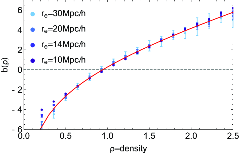
In order to investigate the convergence towards the large-separation limit, we also measure the density bias at different separations resubscript𝑟𝑒r_{e} (see Fig. 5, right-hand panel). For separation larger than 2R1=202subscript𝑅1202R_{1}=20Mpc/habsent/h (adjacent spheres!), the prediction lies within the error bars of the simulations for the full range of density probed (0.2<ρ^<2.50.2^𝜌2.50.2<{\hat{\rho}}<2.5).

Note that appendix D shows that the density bias estimated from the auto-correlation (see equation 47) is fully consistent with the cross-correlation based estimator used in this section.
Refer to caption
Figure 5: The density bias function b(ρ)𝑏𝜌b(\rho) for σ=0.97𝜎0.97\sigma=0.97 measured in our simulation for different separations resubscript𝑟𝑒r_{e} as labelled. The large-separation prediction is displayed in red.

6.2 Slope bias function

In order to measure the slope bias in the simulation, we consider the set of concentric spheres with radii R1=10Mpc/hsubscript𝑅110MpcR_{1}=10{\rm Mpc}/h and R2=11Mpc/hsubscript𝑅211MpcR_{2}=11{\rm Mpc}/h and pairs that are separated by re=20subscript𝑟𝑒20r_{e}=20Mpc/habsent/h so that each set II\rm I of two concentric spheres with density ρIsubscript𝜌I\rho_{\rm I} and slope sIsubscript𝑠Is_{\rm I} has six neighbours at distance resubscript𝑟𝑒r_{e}. Following equation (49), we compute again a sum over each set II\rm I and its 6 neighbouring sets at distance re=20subscript𝑟𝑒20r_{e}=20Mpc/habsent/h labelled with the indices αI,jsubscript𝛼I𝑗\alpha_{{\rm I},j} for 1j61𝑗61\leq j\leq 6

b^(s^)=1ξ^[I,j(s^Δs/2sIs^+Δs/2)ραI,j6I(s^Δs/2sIs^+Δs/2)1],^𝑏^𝑠1^𝜉delimited-[]subscriptIj^𝑠Δ𝑠2subscript𝑠I^𝑠Δ𝑠2subscript𝜌subscript𝛼I𝑗6subscriptI^𝑠Δ𝑠2subscript𝑠I^𝑠Δ𝑠21\hat{b}({\hat{s}})\!=\!\frac{1}{\hat{\xi}}\!\left[\!\frac{\sum_{\rm I,j}{\cal B}({\hat{s}}\!-\!\Delta s/2\leq s_{\rm I}\leq{\hat{s}}\!+\!\Delta s/2)\rho_{\alpha_{{\rm I},j}}}{6\sum_{\rm I}{\cal B}({\hat{s}}-\Delta s/2\leq s_{\rm I}\leq{\hat{s}}+\Delta s/2)}\!-\!1\right]\!, (67)

where the bin width is set to Δs=5/21Δ𝑠521\Delta s=5/21 here.

The slope bias function b(s^)𝑏^𝑠b({\hat{s}}) measured for different values of the variance by means of equation (67) is shown in Fig. 6 and can be compared to the large-deviation prediction displayed with solid lines. The two uncorrelated configurations predicted by our model are recovered around s^±0.5^𝑠plus-or-minus0.5{\hat{s}}\approx\pm 0.5. One could make use of this striking feature in order to minimize large-scale clustering while restricting counts to such slopes according to equation (12)555The correlation vanishes at leading order in our calculations, not taken into account proximity effects and higher order correlation functions.. Predictions and measurements are in good agreement for small slopes |s^|1less-than-or-similar-to^𝑠1|{\hat{s}}|\lesssim 1 and both show that small slope regions are less clustered than sharper environments. They start to depart from one another in the tails of the distribution. Note that already the PDF of the slope shows some level of discrepancy in this regime, which can be due to our numerical integration, our choice of parametrization for the variance (which does not take into account the running of the spectral index) or some unforeseen artifacts from the simulation. Further work is necessary to understand exactly why those discrepancies arise. It is hoped that larger simulations and more robust analytical approximations (following Uhlemann et al., 2015) will resolve these issues.

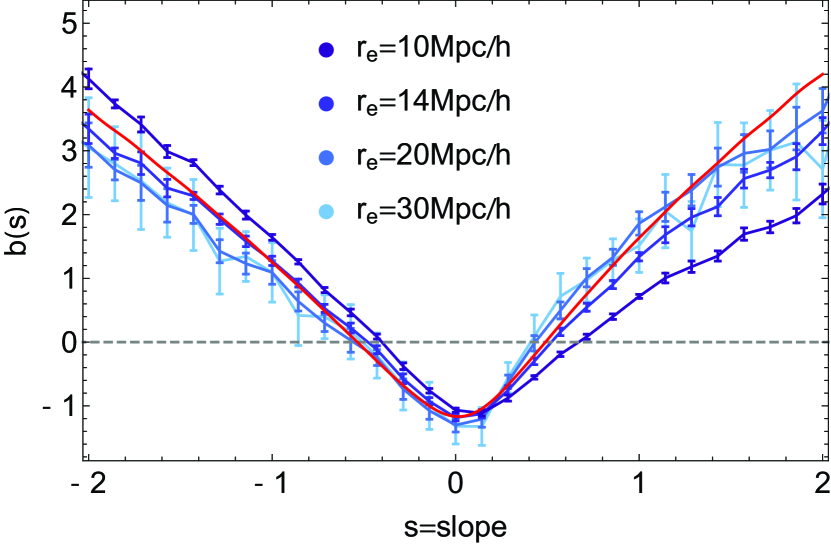
Fig. 7 compares the measurements to the prediction for different values of the separation, re=R1subscript𝑟𝑒subscript𝑅1r_{e}=R_{1}, 2R12subscript𝑅1\sqrt{2}R_{1} (along a diagonal), 2R12subscript𝑅12R_{1}(adjacent cells) and 3R13subscript𝑅13R_{1}. The convergence towards the large-separation prediction (in red) is quick since the prediction starts to deviate from the error bars of the measurements only for re2R1less-than-or-similar-tosubscript𝑟𝑒2subscript𝑅1r_{e}\lesssim 2R_{1} (adjacent cells!). Note that as expected, error bars are larger for larger separations.
Refer to caption
Figure 6: The slope bias b(s^)𝑏^𝑠b({\hat{s}}) for different values of the variance as labelled. Measurements in the simulation for spheres of radii R1=10Mpc/hsubscript𝑅110MpcR_{1}=10{\rm Mpc}/h and R2=11Mpc/hsubscript𝑅211MpcR_{2}=11{\rm Mpc}/h separated by re=20subscript𝑟𝑒20r_{e}=20Mpc/habsent/h using the estimator defined in equation (67) are displayed with error bars and compared with the prediction (solid line).
Refer to caption
Figure 7: The slope bias b(s^)𝑏^𝑠b({\hat{s}}) measured in the simulation at redshift z=0.97𝑧0.97z=0.97 corresponding to σ=0.48𝜎0.48\sigma=0.48 and for different values of the separation from re=R1=10subscript𝑟𝑒subscript𝑅110r_{e}=R_{1}=10Mpc/habsent/h to 3R1=303subscript𝑅1303R_{1}=30Mpc/habsent/h as labelled. The measurements quickly converge towards the predicted large-separation limit (red solid line).

7 Application to cosmic variance

We propose here to illustrate how the large-deviation prediction for the bias can be used to predict the statistics of errors. For that purpose, we measured the density PDF in 253superscript25325^{3} spheres of radius R=10𝑅10R=10Mpc/habsent/h at redshift z=1𝑧1z=1 in our simulation. As already pointed out in Section 2.3, our estimate of the PDF can suffer from two types of errors : shot noise and cosmic variance. We use equation 13 to compute the expected error and display the result in Figure 8. For the particular configuration used here, the cosmic variance is dominant compared to the shot noise error. As expected, error bars obtained by resampling seem to slightly underestimate the error budget. If the distance between the spheres increases, the amount of cosmic variance decreases as the spheres are less correlated. One can anticipate that for a given accessible volume, there is a balance to find between reducing the number of spheres to have them as independent as possible or increasing the number of spheres to reduce the shot noise. Finding the optimal number of spheres and radii to consider for a given survey geometry is left for future works.

8 Conclusion

We have shown how to compute joint statistics of the density within multiple concentric spheres in two regimes : i) the generating function of cumulants containing any powers of concentric densities in one location and one power of density at some arbitrary distance and ii) the two-point correlation function of the density in concentric spheres when the cells are sufficiently well apart. The latter allowed us to estimate the bias and cosmic variance involved in applying standard concentric count-in-cells statistics to cosmological fields of finite extent in that regime. The accuracy of the large-distance approximation was quantified against numerical simulations and shown to be valid even for adjacent cells (20absent20\approx 20Mpc/habsent/h here), strengthening earlier findings by Bernardeau (1996) in the one-cell case. These simulations where also used to assess the validity of the large-deviation principle, which only formally holds in the zero variance limit, but was shown to give accurate predictions even for variance of order unity, in the so-called quasi-linear regime. The bias functions (b(ρ^)𝑏^𝜌b({\hat{\rho}}), b(s^)𝑏^𝑠b({\hat{s}}) in this work) allow us to quantify the covariances expected in finite volume effects, hence build accurate maximum likelihood estimators that could be applied to future surveys. In particular, the shape of b(s^)𝑏^𝑠b({\hat{s}}) we found suggests that tailoring counts to cells which have slopes of the order of ±1/2plus-or-minus12\pm 1/2 could be used to mitigate its effect. The formalism presented here can be straightforwardly extended to predict the bias of multiple concentric spheres including the bias of regions having a given density and slope b(ρ^,s^)𝑏^𝜌^𝑠b({\hat{\rho}},{\hat{s}}).

While the large-deviation predictions of count-in-cell bias functions rely on numerical integration in the complex plane, the recent results of Uhlemann et al. (2015) sets the stage for accurate analytical approximations, using the logarithmic transform of the density. It would therefore be of interest to apply this log-transformation to the two-point statistics presented in this paper. This will be the topic of upcoming work.

It has to be emphasized that the scale-dependence of the count-in-cell bias (that is clearly seen in simulations on scales below 20absent20\approx 20 Mpc/habsent/h) can not be captured by the large-deviation principle used in this work. However, this formalism is a unique opportunity to get insights into the mildly non-linear evolution of halo biasing in contrast to peak models which usually assumes Gaussianity or very recently a Zel’dovich ballistic displacement of the initial peaks (Baldauf et al. (2016), Baldauf et al., in prep). An hybrid analysis between both approaches is challenging but would be of great interest. Building up this peak theory in the large-deviation regime is left for future works.

It would also be worth extending the investigation of biases and cosmic variance to the velocity field following the results obtained by Bernardeau (1992) in the one-point case, and to projected densities.
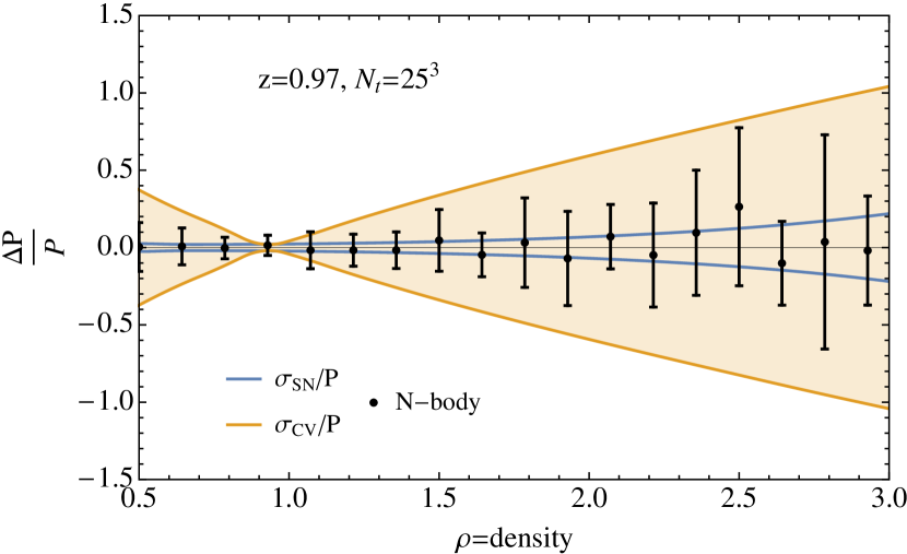
Refer to caption
Figure 8: Expected shot noise (blue) and cosmic variance (yellow) for the density PDF measured from 253superscript25325^{3} spheres of radius R=10𝑅10R=10Mpc/habsent/h at redshift z=1𝑧1z=1 regularly drawn in our simulation. Those predictions are compared with error bars (black) estimated as the standard deviation among eight sub-cubes of the simulation.

Acknowledgements: This work is partially supported by the grants ANR-12-BS05-0002 and ANR-13-BS05-0005 of the French Agence Nationale de la Recherche. The simulations were run on the Horizon cluster. We acknowledge support from S. Rouberol for running the cluster for us and warmly thank Cora Uhlemann for useful comments and careful reading of the manuscript. SC also thanks Marcelo Alvarez and Xin Wang for insightful discussions.

References

  • Abazajian et al. (2003) Abazajian K., Adelman-McCarthy J. K., Agüeros M. A., Allam S. S., Anderson S. F., Annis J., Bahcall N. A., Baldry I. K., Bastian S., Berlind A., et al. 2003, AJ, 126, 2081
  • Akhiezer (1965) Akhiezer N., 1965, The classical moment problem: and some related questions in analysis. University mathematical monographs, Oliver & Boyd
  • Baldauf et al. (2016) Baldauf T., Codis S., Desjacques V., Pichon C., 2016, MNRAS, 456, 3985
  • Baldauf et al. (2012) Baldauf T., Seljak U., Desjacques V., McDonald P., 2012, Phys. Rev. D, 86, 083540
  • Balian & Schaeffer (1989) Balian R., Schaeffer R., 1989, A&A, 220, 1
  • Bardeen et al. (1986) Bardeen J. M., Bond J. R., Kaiser N., Szalay A. S., 1986, ApJ, 304, 15
  • Baugh et al. (1995) Baugh C. M., Gaztanaga E., Efstathiou G., 1995, MNRAS, 274, 1049
  • Bernardeau (1992) Bernardeau F., 1992, ApJ Let., 390, L61
  • Bernardeau (1996) Bernardeau F., 1996, A&A, 312, 11
  • Bernardeau et al. (2015) Bernardeau F., Codis S., Pichon C., 2015, MNRAS, 449, L105
  • Bernardeau et al. (2002) Bernardeau F., Colombi S., Gaztañaga E., Scoccimarro R., 2002, Phys. Rep., 367, 1
  • Bernardeau et al. (2008) Bernardeau F., Crocce M., Scoccimarro R., 2008, Phys. Rev. D, 78, 103521
  • Bernardeau et al. (2014) Bernardeau F., Pichon C., Codis S., 2014, Phys. Rev. D, 90, 103519
  • Bernardeau & Reimberg (2015) Bernardeau F., Reimberg P., 2015, ArXiv e-prints
  • Carron (2011) Carron J., 2011, ApJ, 738, 86
  • Carron & Neyrinck (2012) Carron J., Neyrinck M. C., 2012, ApJ, 750, 28
  • Carron & Szapudi (2015) Carron J., Szapudi I., 2015, ArXiv e-prints
  • Catelan et al. (2000) Catelan P., Porciani C., Kamionkowski M., 2000, MNRAS, 318, L39
  • Coles & Jones (1991) Coles P., Jones B., 1991, MNRAS, 248, 1
  • Colombi et al. (1995) Colombi S., Bouchet F. R., Schaeffer R., 1995, ApJ Sup., 96, 401
  • Crocce et al. (2015) Crocce M., Castander F. J., Gaztañaga E., Fosalba P., Carretero J., 2015, MNRAS, 453, 1513
  • Davis et al. (1985) Davis M., Efstathiou G., Frenk C. S., White S. D. M., 1985, ApJ, 292, 371
  • Dekel & Lahav (1999) Dekel A., Lahav O., 1999, ApJ, 520, 24
  • Dekel & Rees (1987) Dekel A., Rees M. J., 1987, Nature, 326, 455
  • Fry (1996) Fry J. N., 1996, ApJ Let., 461, L65
  • Fry & Gaztañaga (1993) Fry J. N., Gaztañaga E., 1993, ApJ, 413, 447
  • Giannantonio & Porciani (2010) Giannantonio T., Porciani C., 2010, Phys. Rev. D, 81, 063530
  • Guo & Jing (2009) Guo H., Jing Y. P., 2009, ApJ, 702, 425
  • Kaiser (1984) Kaiser N., 1984, ApJ Let., 284, L9
  • Kaiser (1987) Kaiser N., 1987, MNRAS, 227, 1
  • Kiessling et al. (2015) Kiessling A., Cacciato M., Joachimi B., Kirk D., Kitching T. D., Leonard A., Mandelbaum R., Schäfer B. M., Sifón C., Brown M. L., Rassat A., 2015, Space Sci. Rev., 193, 67
  • Komatsu et al. (2011) Komatsu E., Smith K. M., Dunkley J., Bennett C. L., Gold B., Hinshaw G., Jarosik N., Larson D., et al. 2011, ApJ Sup., 192, 18
  • Laureijs et al. (2011) Laureijs R., Amiaux J., Arduini S., Auguères J. ., Brinchmann J., Cole R., Cropper M., Dabin C., Duvet L., Ealet A., et al. 2011, ArXiv e-prints
  • Lazanu et al. (2015) Lazanu A., Giannantonio T., Schmittfull M., Shellard E. P. S., 2015, ArXiv e-prints
  • Levi et al. (2013) Levi M., Bebek C., Beers T., Blum R., Cahn R., Eisenstein D., Flaugher B., Honscheid K., Kron R., Lahav O., McDonald P., Roe N., Schlegel D., representing the DESI collaboration 2013, ArXiv e-prints
  • Ludlow & Porciani (2011) Ludlow A. D., Porciani C., 2011, MNRAS, 413, 1961
  • Lumsden et al. (1989) Lumsden S. L., Heavens A. F., Peacock J. A., 1989, MNRAS, 238, 293
  • Manera & Gaztañaga (2011) Manera M., Gaztañaga E., 2011, MNRAS, 415, 383
  • Maurogordato & Lachieze-Rey (1987) Maurogordato S., Lachieze-Rey M., 1987, ApJ, 320, 13
  • McDonald & Roy (2009) McDonald P., Roy A., 2009, JCAP , 8, 020
  • Mirbabayi et al. (2015) Mirbabayi M., Schmidt F., Zaldarriaga M., 2015, JCAP , 7, 030
  • Moster et al. (2011) Moster B. P., Somerville R. S., Newman J. A., Rix H.-W., 2011, ApJ, 731, 113
  • Nusser & Davis (1994) Nusser A., Davis M., 1994, ApJ Let., 421, L1
  • Pen (1998) Pen U.-L., 1998, ApJ, 504, 601
  • Prunet et al. (2008) Prunet S., Pichon C., Aubert D., Pogosyan D., Teyssier R., Gottloeber S., 2008, ApJ Sup., 178, 179
  • Sánchez et al. (2014) Sánchez C., Carrasco Kind M., Lin H., Miquel R., Abdalla F. B., Amara A., 2014, MNRAS, 445, 1482
  • Schneider & Teyssier (2015) Schneider A., Teyssier R., 2015, JCAP , 12, 049
  • Scoccimarro et al. (1998) Scoccimarro R., Colombi S., Fry J. N., Frieman J. A., Hivon E., Melott A., 1998, ApJ, 496, 586
  • Senatore (2015) Senatore L., 2015, JCAP , 11, 007
  • Springel (2005) Springel V., 2005, MNRAS, 364, 1105
  • Szapudi & Colombi (1996) Szapudi I., Colombi S., 1996, ApJ, 470, 131
  • Szapudi et al. (1999) Szapudi I., Colombi S., Bernardeau F., 1999, MNRAS, 310, 428
  • Taruya et al. (2010) Taruya A., Nishimichi T., Saito S., 2010, Phys. Rev. D, 82, 063522
  • Tegmark & Peebles (1998) Tegmark M., Peebles P. J. E., 1998, ApJ Let., 500, L79
  • Touchette (2011) Touchette H., 2011, ArXiv e-prints
  • Uhlemann et al. (2015) Uhlemann C., Codis S., Pichon C., Bernardeau F., Reimberg P., 2015, ArXiv e-prints
  • Valageas (2002) Valageas P., 2002, A&A, 382, 412

Appendix A Radii decimations

The purpose of this appendix is to insure that the expression of the cumulant generating function φ({λ})𝜑𝜆\varphi(\{\lambda\}), given by equation (19), is consistent with variable decimation, i.e. we want to check that

φ({λ1,,λn})=φ({λ1,,λn,λn+1=0,,λn+m=0}),\varphi(\{\lambda_{1},\dots,\lambda_{n}\})=\\ \varphi(\{\lambda_{1},\dots,\lambda_{n},\lambda_{n+1}=0,\dots,\lambda_{n+m}=0\})\,, (68)

where the left-hand side is computed from n𝑛n cells whereas the right-hand side is computed with n+m𝑛𝑚n+m cells. This property was also studied in BPC but we propose here a slightly different proof and we will make use of some of the results – in particular equation (81) – in the main text.

By mathematical induction, it is sufficient to prove equation (68) when m𝑚m is set to 1. We will therefore show here that the following property holds

φ({λ1,,λn})=φ({λ1,,λn,λn+1=0}),𝜑subscript𝜆1subscript𝜆𝑛𝜑subscript𝜆1subscript𝜆𝑛subscript𝜆𝑛10\varphi(\{\lambda_{1},\dots,\lambda_{n}\})=\varphi(\{\lambda_{1},\dots,\lambda_{n},\lambda_{n+1}=0\})\,, (69)

where the left-hand side is still computed from n𝑛n cells whereas the right-hand side is now computed with n+1𝑛1n+1 cells.

Let us define a set 𝒜𝒜{\cal A} of n𝑛n cells and a set {\cal B} of m=1𝑚1m=1 cell. One can then define the covariance matrix ΣΣ\Sigma defined by Σij=σ2(Riζ(τi)1/3,Rjζ(τj)1/3)subscriptΣ𝑖𝑗superscript𝜎2subscript𝑅𝑖𝜁superscriptsubscript𝜏𝑖13subscript𝑅𝑗𝜁superscriptsubscript𝜏𝑗13\Sigma_{ij}=\sigma^{2}(R_{i}\zeta(\tau_{i})^{1/3},R_{j}\zeta(\tau_{j})^{1/3}) between two any cells of the union of 𝒜𝒜{\cal A} and {\cal B}. The covariance matrix restricted to 𝒜𝒜{\cal A} will be denoted Σ~=Σ|𝒜\tilde{\Sigma}=\Sigma_{|{\cal A}}. For the sake of clarity, in this appendix, greeks indices refer to the set 𝒜𝒜{\cal A} and therefore go between 1 and n𝑛n and a tilde is displayed over the corresponding operators while in 𝒜𝒜{\cal A}\cup{\cal B} we use roman indices which go between 1 and n+1𝑛1n+1 and no tilde.

The cumulant generating functions for the n𝑛n cells in 𝒜𝒜{\cal A} is given by

φ({λ1,,λn})=λμρ~μ12Ξ~μντ~μτ~ν,𝜑subscript𝜆1subscript𝜆𝑛subscript𝜆𝜇subscript~𝜌𝜇12subscript~Ξ𝜇𝜈subscript~𝜏𝜇subscript~𝜏𝜈\varphi(\{\lambda_{1},\dots,\lambda_{n}\})=\lambda_{\mu}\tilde{\rho}_{\mu}-\frac{1}{2}\tilde{\Xi}_{\mu\nu}\tilde{\tau}_{\mu}\tilde{\tau}_{\nu}\,, (70)

with the stationary conditions

λκ=Ψ~ρ~k=Ξ~μκτ~μdτ~κdρ~κ+12Ξ~μνρ~κτ~μτ~ν,subscript𝜆𝜅~Ψsubscript~𝜌𝑘subscript~Ξ𝜇𝜅subscript~𝜏𝜇dsubscript~𝜏𝜅dsubscript~𝜌𝜅12subscript~Ξ𝜇𝜈subscript~𝜌𝜅subscript~𝜏𝜇subscript~𝜏𝜈\lambda_{\kappa}=\frac{\partial\tilde{\Psi}}{\partial\tilde{\rho}_{k}}=\tilde{\Xi}_{\mu\kappa}\tilde{\tau}_{\mu}\frac{\hbox{d}\tilde{\tau}_{\kappa}}{\hbox{d}\tilde{\rho}_{\kappa}}+\frac{1}{2}\frac{\partial\tilde{\Xi}_{\mu\nu}}{\partial\tilde{\rho}_{\kappa}}\tilde{\tau}_{\mu}\tilde{\tau}_{\nu}, (71)

where Ξ~~Ξ\tilde{\Xi} is the inverse matrix of Σ~~Σ\tilde{\Sigma} and we use implicit summations over repeated indices μ,ν𝜇𝜈\mu,\nu between 1 and n𝑛n.

Our purpose is to show that it is identical to the expression of φ({λi}1in+1)𝜑subscriptsubscript𝜆𝑖1𝑖𝑛1\varphi(\{\lambda_{i}\}_{1\leq i\leq n+1}) describing the cumulant generating function of the n+1𝑛1n+1 cells when the last value λn+1subscript𝜆𝑛1\lambda_{n+1} is set to zero. In this latter case we have

φ({λ1,,λn,0})=λμρμ12Ξijτiτj,𝜑subscript𝜆1subscript𝜆𝑛0subscript𝜆𝜇subscript𝜌𝜇12subscriptΞ𝑖𝑗subscript𝜏𝑖subscript𝜏𝑗\varphi(\{\lambda_{1},\dots,\lambda_{n},0\})=\lambda_{\mu}\rho_{\mu}-\frac{1}{2}\Xi_{ij}\tau_{i}\tau_{j}\,, (72)

with the stationary conditions

λκsubscript𝜆𝜅\displaystyle\lambda_{\kappa} =\displaystyle= Ξiκτidτκdρκ+12Ξijρκτiτj;subscriptΞ𝑖𝜅subscript𝜏𝑖dsubscript𝜏𝜅dsubscript𝜌𝜅12subscriptΞ𝑖𝑗subscript𝜌𝜅subscript𝜏𝑖subscript𝜏𝑗\displaystyle\Xi_{i\kappa}\tau_{i}\frac{\hbox{d}\tau_{\kappa}}{\hbox{d}\rho_{\kappa}}+\frac{1}{2}\frac{\partial\Xi_{ij}}{\partial\rho_{\kappa}}\tau_{i}\tau_{j}; (73)
λn+1=0subscript𝜆𝑛10\displaystyle\lambda_{n+1}=0 =\displaystyle= Ξn+1iτidτn+1dρn+1+12Ξijρn+1τiτj,subscriptΞ𝑛1𝑖subscript𝜏𝑖dsubscript𝜏𝑛1dsubscript𝜌𝑛112subscriptΞ𝑖𝑗subscript𝜌𝑛1subscript𝜏𝑖subscript𝜏𝑗\displaystyle\Xi_{n+1i}\tau_{i}\frac{\hbox{d}\tau_{n+1}}{\hbox{d}\rho_{n+1}}+\frac{1}{2}\frac{\partial\Xi_{ij}}{\partial\rho_{n+1}}\tau_{i}\tau_{j}\,, (74)

with implicit summations over i,j𝑖𝑗i,j between 1 and n+1𝑛1n+1. The constraint (74) allows one to determine the value of τn+1subscript𝜏𝑛1\tau_{n+1} in terms of τνsubscript𝜏𝜈\tau_{\nu}. To do so, let us first express Ξij/ρisubscriptΞ𝑖𝑗subscript𝜌𝑖\partial\Xi_{ij}/\partial\rho_{i} as a function of the derivatives of ΣΣ\Sigma. By differentiating ΞΣ=𝕀ΞΣ𝕀\Xi\cdot\Sigma=\mathbb{I}, we get

Ξρi=ΞΣρiΞ.Ξsubscript𝜌𝑖ΞΣsubscript𝜌𝑖Ξ\frac{\partial\Xi}{\partial\rho_{i}}=-\Xi\cdot\frac{\partial\Sigma}{\partial\rho_{i}}\cdot\Xi\,. (75)

One can also write this relation when the inverse matrix Ξ~~Ξ\tilde{\Xi} is defined from the covariance matrix of the cells restricted in 𝒜𝒜{\cal A} only, Σ~~Σ\tilde{\Sigma},

Ξ~ρ~κ=Ξ~Σ~ρ~κΞ~.~Ξsubscript~𝜌𝜅~Ξ~Σsubscript~𝜌𝜅~Ξ\frac{\partial\tilde{\Xi}}{\partial\tilde{\rho}_{\kappa}}=-\tilde{\Xi}\cdot\frac{\partial\tilde{\Sigma}}{\partial\tilde{\rho}_{\kappa}}\cdot\tilde{\Xi}\,. (76)

Substituting V=Ξτ𝑉Ξ𝜏V=\Xi\cdot\tau and V~=Ξ~τ~~𝑉~Ξ~𝜏\tilde{V}=\tilde{\Xi}\cdot\tilde{\tau} into equations (71), (73), (74), we get

λκsubscript𝜆𝜅\displaystyle\lambda_{\kappa} =\displaystyle= V~κdτ~κdρ~κ12V~tΣ~ρ~κV~,subscript~𝑉𝜅dsubscript~𝜏𝜅dsubscript~𝜌𝜅12superscript~𝑉𝑡~Σsubscript~𝜌𝜅~𝑉\displaystyle\tilde{V}_{\kappa}\frac{\hbox{d}\tilde{\tau}_{\kappa}}{\hbox{d}\tilde{\rho}_{\kappa}}-\frac{1}{2}\tilde{V}^{t}\cdot\frac{\partial\tilde{\Sigma}}{\partial\tilde{\rho}_{\kappa}}\cdot\tilde{V}, (77)
λκsubscript𝜆𝜅\displaystyle\lambda_{\kappa} =\displaystyle= Vκdτκdρκ12VtΣρκV,subscript𝑉𝜅dsubscript𝜏𝜅dsubscript𝜌𝜅12superscript𝑉𝑡Σsubscript𝜌𝜅𝑉\displaystyle V_{\kappa}\frac{\hbox{d}\tau_{\kappa}}{\hbox{d}\rho_{\kappa}}-\frac{1}{2}V^{t}\cdot\frac{\partial\Sigma}{\partial\rho_{\kappa}}\cdot V, (78)
00\displaystyle 0 =\displaystyle= Vn+1dτn+1dρn+112VtΣρn+1V.subscript𝑉𝑛1dsubscript𝜏𝑛1dsubscript𝜌𝑛112superscript𝑉𝑡Σsubscript𝜌𝑛1𝑉\displaystyle V_{n+1}\frac{\hbox{d}\tau_{n+1}}{\hbox{d}\rho_{n+1}}-\frac{1}{2}V^{t}\cdot\frac{\partial\Sigma}{\partial\rho_{n+1}}\cdot V\,. (79)

An obvious solution to this set of equations is given by

Vμ=V~μ,Vn+1=0.formulae-sequencesubscript𝑉𝜇subscript~𝑉𝜇subscript𝑉𝑛10V_{\mu}=\tilde{V}_{\mu}\,,\,V_{n+1}=0. (80)

Indeed, in that case, using i=/ρisubscript𝑖subscript𝜌𝑖\partial_{i}=\partial/\partial\rho_{i} and ~κ=/ρ~κsubscript~𝜅subscript~𝜌𝜅\tilde{\partial}_{\kappa}=\partial/\partial\tilde{\rho}_{\kappa}, we have Vκ(dκτκ)=V~κ(d~κτ~κ)subscript𝑉𝜅subscriptd𝜅subscript𝜏𝜅subscript~𝑉𝜅subscript~d𝜅subscript~𝜏𝜅V_{\kappa}(\hbox{d}_{\kappa}\tau_{\kappa})=\tilde{V}_{\kappa}(\tilde{\hbox{d}}_{\kappa}\tilde{\tau}_{\kappa}), VtκΣV=V~t~κΣ~V~+0superscript𝑉𝑡subscript𝜅Σ𝑉superscript~𝑉𝑡subscript~𝜅~Σ~𝑉0V^{t}\cdot\partial_{\kappa}\Sigma\cdot V=\tilde{V}^{t}\cdot\tilde{\partial}_{\kappa}\tilde{\Sigma}\cdot\tilde{V}+0 and Vtn+1ΣV=0superscript𝑉𝑡subscript𝑛1Σ𝑉0V^{t}\cdot\partial_{n+1}\Sigma\cdot V=0 because ΣijsubscriptΣ𝑖𝑗\Sigma_{ij} solely depends on the densities ρisubscript𝜌𝑖\rho_{i} and ρjsubscript𝜌𝑗\rho_{j}.

The solution given by equation (80) is equivalent to

τμ=τ~μ,τn+1=Ξμn+1Ξn+1n+1τ~μ=σn+1μΞ~μντ~ν.formulae-sequencesubscript𝜏𝜇subscript~𝜏𝜇subscript𝜏𝑛1subscriptΞ𝜇𝑛1subscriptΞ𝑛1𝑛1subscript~𝜏𝜇subscript𝜎𝑛1𝜇subscript~Ξ𝜇𝜈subscript~𝜏𝜈\tau_{\mu}=\tilde{\tau}_{\mu}\,,\,\tau_{n+1}=-\frac{\Xi_{\mu\,n+1}}{\Xi_{n+1\,n+1}}\tilde{\tau}_{\mu}=\sigma_{n+1\,\mu}\tilde{\Xi}_{\mu\nu}\tilde{\tau}_{\nu}\,. (81)

We then immediately get

λμρμ=λμρ~μ,12τiVi=12τ~νV~ν,formulae-sequencesubscript𝜆𝜇subscript𝜌𝜇subscript𝜆𝜇subscript~𝜌𝜇12subscript𝜏𝑖subscript𝑉𝑖12subscript~𝜏𝜈subscript~𝑉𝜈\lambda_{\mu}\rho_{\mu}=\lambda_{\mu}\tilde{\rho}_{\mu}\,,\,\frac{1}{2}\tau_{i}V_{i}=\frac{1}{2}\tilde{\tau}_{\nu}\tilde{V}_{\nu}\,, (82)

so that the property given by equation (69), namely φ({λ1,,λn})=φ({λ1,,λn,λn+1=0})𝜑subscript𝜆1subscript𝜆𝑛𝜑subscript𝜆1subscript𝜆𝑛subscript𝜆𝑛10\varphi(\{\lambda_{1},\dots,\lambda_{n}\})=\varphi(\{\lambda_{1},\dots,\lambda_{n},\lambda_{n+1}=0\}), is established. Note that the same argument holds for the bias function so that bφ(λ1,,λn)=bφ(λ1,,λn,0)subscript𝑏𝜑subscript𝜆1subscript𝜆𝑛subscript𝑏𝜑subscript𝜆1subscript𝜆𝑛0b_{\varphi}(\lambda_{1},\dots,\lambda_{n})=b_{\varphi}(\lambda_{1},\dots,\lambda_{n},0).

Appendix B Large distance limit

Let us present an heuristic demonstration of the property (38). The argument is based on a peak-background type construction. So let us consider a functional i[ρ(x);x1]subscript𝑖𝜌xsubscriptx1{\cal{F}}_{i}[\rho(\textbf{x});\textbf{x}_{1}] of the density field ρ(x)𝜌x\rho(\textbf{x}) in the vicinity of the location x1subscriptx1\textbf{x}_{1}. The idea is that i[ρ(x);x1]subscript𝑖𝜌xsubscriptx1{\cal{F}}_{i}[\rho(\textbf{x});\textbf{x}_{1}] depends on ρ(x)𝜌x\rho(\textbf{x}) only when |xx1|xsubscriptx1|\textbf{x}-\textbf{x}_{1}| is small enough, say |xx1|xsubscriptx1|\textbf{x}-\textbf{x}_{1}|\leq{\cal{R}} and we are interested in how i[ρ(x);x1]subscript𝑖𝜌xsubscriptx1{\cal{F}}_{i}[\rho(\textbf{x});\textbf{x}_{1}] and i[ρ(x);x2]subscript𝑖𝜌xsubscriptx2{\cal{F}}_{i}[\rho(\textbf{x});\textbf{x}_{2}] are correlated when |x1x2|Rmuch-greater-thansubscriptx1subscriptx2𝑅|\textbf{x}_{1}-\textbf{x}_{2}|\gg R. One can then say that the density field values at large separation are correlated only through the large scale fluctuations, or more precisely through the response function of the functional {\cal{F}} to large scale density fluctuations. We assume the latter to be in the linear regime and we note them δL(x)subscript𝛿𝐿x\delta_{L}(\textbf{x}). Note that ρ(x)𝜌x\rho(\textbf{x}) is a non trivial functional of δL(x)subscript𝛿𝐿x\delta_{L}(\textbf{x}) through mode coupling. Formally in the vicinity of x1subscriptx1\textbf{x}_{1} for instance we could write

ρ(x)=ρS(x)+𝒟[ρ(x);x1]δ(x1)+.𝜌xsubscript𝜌𝑆xsubscript𝒟𝜌xsubscriptx1subscript𝛿subscriptx1\rho(\textbf{x})=\rho_{S}(\textbf{x})+{\cal D}_{{\cal{L}}}[\rho(\textbf{x});\textbf{x}_{1}]\delta_{{\cal{L}}}(\textbf{x}_{1})+\dots. (83)

where ρS(x)subscript𝜌𝑆x\rho_{S}(\textbf{x}) is the value of the field when long wave modes have been suppressed and where 𝒟[ρ(x);x1]subscript𝒟𝜌xsubscriptx1{\cal D}_{{\cal{L}}}[\rho(\textbf{x});\textbf{x}_{1}] gives the linear response function of the field ρ(x)𝜌x\rho(\textbf{x}) to the large scale fluctuation δsubscript𝛿\delta_{{\cal{L}}} in the vicinity of x1subscriptx1\textbf{x}_{1}. Then any functional [ρ(x);x1]𝜌xsubscriptx1{\cal{F}}[\rho(\textbf{x});\textbf{x}_{1}] of the density field can be similarly expanded as a function of the local density contrast

[ρ(x);x1]=[ρS(x);x1]+𝒟[[ρ(x)];x1]δ(x1)+.𝜌xsubscriptx1subscript𝜌𝑆xsubscriptx1subscript𝒟delimited-[]𝜌xsubscriptx1subscript𝛿subscriptx1{\cal{F}}[\rho(\textbf{x});\textbf{x}_{1}]={\cal{F}}[\rho_{S}(\textbf{x});\textbf{x}_{1}]+{\cal D}_{{\cal{L}}}[{\cal{F}}[\rho(\textbf{x})];\textbf{x}_{1}]\delta_{{\cal{L}}}(\textbf{x}_{1})+\dots. (84)

Note that in this expression both [ρS(x);x1]subscript𝜌𝑆xsubscriptx1{\cal{F}}[\rho_{S}(\textbf{x});\textbf{x}_{1}] and 𝒟[[ρ(x)];x1]subscript𝒟delimited-[]𝜌xsubscriptx1{\cal D}_{{\cal{L}}}[{\cal{F}}[\rho(\textbf{x})];\textbf{x}_{1}] are random quantities that depend on the small scale density fluctuations, independently on the long wave modes collected in δ(x1)subscript𝛿subscriptx1\delta_{{\cal{L}}}(\textbf{x}_{1}). When taking ensemble average of combination of such quantities, one can observe that

[ρ(x);x1]=[ρS(x)]delimited-⟨⟩𝜌xsubscriptx1delimited-⟨⟩delimited-[]subscript𝜌𝑆x\langle{\cal{F}}[\rho(\textbf{x});\textbf{x}_{1}]\rangle=\langle{\cal{F}}[\rho_{S}(\textbf{x})]\rangle (85)

at dominant order in δsubscript𝛿\delta_{{\cal{L}}} and then that

[ρ(x);x1]ρ(x2)delimited-⟨⟩𝜌xsubscriptx1𝜌subscriptx2\displaystyle\langle{\cal{F}}[\rho(\textbf{x});\textbf{x}_{1}]\ \rho(\textbf{x}_{2})\rangle =\displaystyle= [ρS(x);x1]delimited-⟨⟩subscript𝜌𝑆xsubscriptx1\displaystyle\langle{\cal{F}}[\rho_{S}(\textbf{x});\textbf{x}_{1}]\rangle (86)
+𝒟[[ρS(x)];x1]ξ(x1,x2)delimited-⟨⟩subscript𝒟delimited-[]subscript𝜌𝑆xsubscriptx1subscript𝜉subscriptx1subscriptx2\displaystyle+\ \langle{\cal D}_{{\cal{L}}}[{\cal{F}}[\rho_{S}(\textbf{x})];\textbf{x}_{1}]\rangle\ \xi_{{\cal{L}}}(\textbf{x}_{1},\textbf{x}_{2})
+\displaystyle+\ \dots

where

ξ(x1,x2)δ(x1)δ(x2).subscript𝜉subscriptx1subscriptx2delimited-⟨⟩subscript𝛿subscriptx1subscript𝛿subscriptx2\xi_{{\cal{L}}}(\textbf{x}_{1},\textbf{x}_{2})\equiv\langle\delta_{{\cal{L}}}(\textbf{x}_{1})\ \delta_{{\cal{L}}}(\textbf{x}_{2})\rangle. (87)

The key point is to further observe that,

[ρ(x);x1][ρ(x);x2]delimited-⟨⟩𝜌xsubscriptx1𝜌xsubscriptx2\displaystyle\langle{\cal{F}}[\rho(\textbf{x});\textbf{x}_{1}]\ {\cal{F}}[\rho(\textbf{x});\textbf{x}_{2}]\rangle =\displaystyle= (88)
[ρS(x);x1][ρS(x);x2]delimited-⟨⟩subscript𝜌𝑆xsubscriptx1delimited-⟨⟩subscript𝜌𝑆xsubscriptx2\displaystyle\langle{\cal{F}}[\rho_{S}(\textbf{x});\textbf{x}_{1}]\rangle\langle{\cal{F}}[\rho_{S}(\textbf{x});\textbf{x}_{2}]\rangle
+𝒟[[ρS(x)];x1]𝒟[[ρS(x)];x2]ξ(x1,x2)delimited-⟨⟩subscript𝒟delimited-[]subscript𝜌𝑆xsubscriptx1delimited-⟨⟩subscript𝒟delimited-[]subscript𝜌𝑆xsubscriptx2subscript𝜉subscriptx1subscriptx2\displaystyle+\langle{\cal D}_{{\cal{L}}}[{\cal{F}}[\rho_{S}(\textbf{x})];\textbf{x}_{1}]\rangle\ \langle{\cal D}_{{\cal{L}}}[{\cal{F}}[\rho_{S}(\textbf{x})];\textbf{x}_{2}]\rangle\ \xi_{{\cal{L}}}(\textbf{x}_{1},\textbf{x}_{2})
+\displaystyle+\ \dots

When taking the connected part of these moments, these forms lead to the functional relation,

[ρ(x);x1][ρ(x);x2]csubscriptdelimited-⟨⟩𝜌xsubscriptx1𝜌xsubscriptx2𝑐\displaystyle\langle{\cal{F}}[\rho(\textbf{x});\textbf{x}_{1}]\ {\cal{F}}[\rho(\textbf{x});\textbf{x}_{2}]\rangle_{c} =\displaystyle= 1ξ(x1,x2)1subscript𝜉subscriptx1subscriptx2\displaystyle\frac{1}{\xi_{{\cal{L}}}(\textbf{x}_{1},\textbf{x}_{2})} (89)
×[ρ(x);x1]ρ(x2)c[ρ(x);x2]ρ(x1)c.absentsubscriptdelimited-⟨⟩𝜌xsubscriptx1𝜌subscriptx2𝑐subscriptdelimited-⟨⟩𝜌xsubscriptx2𝜌subscriptx1𝑐\displaystyle\times\langle{\cal{F}}[\rho(\textbf{x});\textbf{x}_{1}]\ \rho(\textbf{x}_{2})\rangle_{c}\langle{\cal{F}}[\rho(\textbf{x});\textbf{x}_{2}]\ \rho(\textbf{x}_{1})\rangle_{c}.

Note that it can easily be extended to two different functionals of the density field and when applied to products of density fields, it precisely leads to the relation (38). This construction actually reproduces the expansion scheme developed in Bernardeau et al. (2008) in Fourier space. In this context the 𝒟[[ρS(x)];x1]delimited-⟨⟩subscript𝒟delimited-[]subscript𝜌𝑆xsubscriptx1\langle{\cal D}_{{\cal{L}}}[{\cal{F}}[\rho_{S}(\textbf{x})];\textbf{x}_{1}]\rangle is simply the nonlinear propagator in real space. The relation (88) could be extended to higher order contributions provided one knew how to compute multi-point propagators.

Appendix C Cosmic error statistics

In this section, we show how to go from equation (5) to the cosmic variance of discrete counts. Hence let us assume that the joint PDF of the density in NtsubscriptNt\rm N_{t} cells reads

𝒫({ρ^1},,{ρ^Nt})=I=1Nt𝒫(ρ^I)[1+i<jb(ρ^I)b(ρ^J)ξIJ].𝒫subscript^𝜌1subscript^𝜌subscriptNtsuperscriptsubscriptproductI1subscriptNt𝒫subscript^𝜌Idelimited-[]1subscriptij𝑏subscript^𝜌I𝑏subscript^𝜌Jsubscript𝜉IJ{\cal P}(\{{\hat{\rho}}_{1}\},\dots,\{{\hat{\rho}}_{\rm N_{t}}\})=\prod_{\rm I=1}^{\rm N_{t}}{\cal P}({\hat{\rho}}_{\rm I})\left[1+\ \sum_{\mathrm{\rm i<j}}b({\hat{\rho}}_{\rm I})b({\hat{\rho}}_{\rm J})\xi_{\rm IJ}\right]\,. (90)

In what follows, we will take ξIJ=ξsubscript𝜉IJ𝜉\xi_{\rm IJ}=\xi independent from the positions and we will denote the density bias bI=b(ρ^I)subscript𝑏I𝑏subscript^𝜌Ib_{\rm I}=b({\hat{\rho}}_{\rm I}).

C.1 The one-cell count-in-cell PDF

We want to estimate 𝒫(ρ^)dρ^𝒫^𝜌d^𝜌{\cal P}(\hat{\rho})\hbox{d}\hat{\rho} by measuring the density in NtsubscriptNt{\rm N_{t}} spheres of same radius R𝑅R. If the spheres are independent i.e there is no bias in the measure bI=0subscript𝑏I0b_{\rm I}=0, then the probability of having N spheres with density ρ^±Δρ/2plus-or-minus^𝜌Δ𝜌2\hat{\rho}\pm\Delta\rho/2 is simply given by a binomial distribution

Punbiased(N)=(NtN)pN(1p)NtN,superscript𝑃unbiasedNsubscriptNtNsuperscript𝑝Nsuperscript1𝑝subscriptNtNP^{\rm{unbiased}}({\rm N})=\left(\!\begin{array}[]{c}{\rm N_{t}}\\ {\rm N}\\ \end{array}\!\right)p^{\rm N}(1-p)^{\rm N_{t}-N}\,, (91)

with (NtN)=Nt!/N!/(NtN)!subscriptNtNsubscriptNtNsubscriptNtN\left(\!\begin{array}[]{c}\rm N_{t}\\ \rm N\\ \end{array}\!\right)=\rm N_{t}!/N!/(N_{t}-N)! and p𝑝p, the probability for the density of one sphere to be in Δ^=[ρ^Δρ/2,ρ^+Δρ/2]^Δ^𝜌Δ𝜌2^𝜌Δ𝜌2\hat{\Delta}=[\hat{\rho}-\Delta\rho/2,\hat{\rho}+\Delta\rho/2], is given by

p=Δ^dρ𝒫(ρ).𝑝subscript^Δd𝜌𝒫𝜌p=\int_{\hat{\Delta}}\hbox{d}\rho\,{\cal P}(\rho)\,. (92)

In the Poisson limit (where NtNmuch-greater-thansubscriptNtN\rm N_{t}\gg N and pNt𝑝subscriptNtp\rm N_{t} is constant), using the Stirling formula x!2πx(x/e)x𝑥2𝜋𝑥superscript𝑥𝑒𝑥x!\approx\sqrt{2\pi x}\left({x}/e\right)^{x} when x𝑥x goes to infinity, this probability distribution trivially becomes a Poisson distribution parametrized by N¯=pNt¯N𝑝subscriptNt{\rm\bar{N}}=p\rm N_{t}

Punbiased(N)N¯NN!exp(N¯).superscript𝑃unbiasedNsuperscript¯NNN¯NP^{\rm{unbiased}}(\rm N)\approx\rm\frac{\bar{N}^{N}}{N!}\exp(-\bar{N})\,. (93)

Accounting for a non-zero bias in equation 90, the probability of having N spheres with density in Δ^=ρ^±Δρ/2^Δplus-or-minus^𝜌Δ𝜌2\hat{\Delta}=\hat{\rho}\pm\Delta\rho/2 becomes

Pbiased(N)=(NtN)P(ρ^1,,ρ^NΔ^ρ^N+1,,ρ^NtΔ^),superscript𝑃biasedNsubscriptNtN𝑃subscript^𝜌1subscript^𝜌N^Δsubscript^𝜌N1subscript^𝜌subscriptNt^ΔP^{\rm{biased}}({\rm N})\!=\!\!\left(\!\!\!\begin{array}[]{c}\rm N_{t}\\ \rm N\\ \end{array}\!\!\!\!\right)P\!\!\left(\!\!\!\begin{array}[]{c}{\hat{\rho}}_{1},\!\dots\!,{\hat{\rho}}_{\rm N}\in\hat{\Delta}\\ {\hat{\rho}}_{\rm N+1},\!\dots\!,{\hat{\rho}}_{\rm N_{t}}\notin\hat{\Delta}\\ \end{array}\!\!\!\!\right), (94)

where the probability of having only the first N densities in Δ^^Δ\hat{\Delta} reads

P(ρ^1,,ρ^NΔ^ρ^N+1,,ρ^NtΔ^)=(Δ^)Ndρ^1dρ^N(+/Δ^)NtNdρ^N+1dρ^Nt𝒫(ρ^1,,ρ^Nt).𝑃subscript^𝜌1subscript^𝜌N^Δsubscript^𝜌N1subscript^𝜌subscriptNt^Δsuperscriptsubscript^ΔNdsubscript^𝜌1dsubscript^𝜌Nsuperscriptsubscriptsubscript^ΔsubscriptNtNdsubscript^𝜌N1dsubscript^𝜌subscriptNt𝒫subscript^𝜌1subscript^𝜌subscriptNtP\!\!\left(\!\!\!\begin{array}[]{c}{\hat{\rho}}_{1},\!\dots\!,{\hat{\rho}}_{\rm N}\in\hat{\Delta}\\ {\hat{\rho}}_{\rm N+1},\!\dots\!,{\hat{\rho}}_{\rm N_{t}}\notin\hat{\Delta}\\ \end{array}\!\!\!\!\right)=\\ \left(\int_{\hat{\Delta}}\right)^{\!\!\!\rm N}\!\!\hbox{d}{\hat{\rho}}_{1}\!\cdots\!\hbox{d}{\hat{\rho}}_{\rm N}\!\left(\!\int_{\mathbb{R}_{+}/\hat{\Delta}}\!\right)^{\!\!\!\rm N_{t}-N}\!\!\!\!\!\!\!\!\!\!\!\!\hbox{d}{\hat{\rho}}_{\rm N+1}\!\cdots\!\hbox{d}{\hat{\rho}}_{\rm N_{t}}{\cal P}({\hat{\rho}}_{1},\dots,{\hat{\rho}}_{\rm N_{t}}). (95)

Given equation (90), equation (94) eventually yields

Pbiased(N)superscript𝑃biasedN\displaystyle P^{\textrm{biased}}(\rm N) =(NtN)×[pN(1p)NtN\displaystyle=\left(\!\begin{array}[]{c}\rm N_{t}\\ \rm N\\ \end{array}\!\right)\times\left[p^{\rm N}(1-p)^{\rm N_{t}-N}\right. (98)
+\displaystyle+ ξN(N1)2(pb)2pN2(1p)NtN𝜉NN12superscript𝑝𝑏2superscript𝑝N2superscript1𝑝subscriptNtN\displaystyle\xi\frac{\rm N(N-1)}{2}(pb)^{2}p^{\rm N-2}(1-p)^{\rm N_{t}-N}
+\displaystyle+ ξN(NtN)pN1pb(pb)(1p)NtN1𝜉NsubscriptNtNsuperscript𝑝N1𝑝𝑏𝑝𝑏superscript1𝑝subscriptNtN1\displaystyle\xi{\rm N(N_{t}-N)}p^{\rm N-1}pb(-pb)(1-p)^{\rm N_{t}-N-1}
+\displaystyle+ ξ(NtN)(NtN1)2pN(pb)2(1p)NtN2],\displaystyle\xi\frac{\rm(N_{t}-N)(N_{t}-N-1)}{2}p^{\rm N}(-pb)^{2}\left.(1-p)^{\rm N_{t}-N-2}\right],

where we introduced pb𝑝𝑏pb such that

pb=Δ^dρ^𝒫(ρ^)b(ρ^)𝑝𝑏subscript^Δd^𝜌𝒫^𝜌𝑏^𝜌pb=\int_{\hat{\Delta}}\hbox{d}{\hat{\rho}}\,{\cal P}({\hat{\rho}})b({\hat{\rho}}) (99)

that comes with complement pb𝑝𝑏-pb as the normalisation of 𝒫𝒫{\cal P} enforces +dρ^𝒫(ρ^)b(ρ^)=0subscriptsubscriptd^𝜌𝒫^𝜌𝑏^𝜌0\int_{\mathbb{R}_{+}}\hbox{d}{\hat{\rho}}\,{\cal P}({\hat{\rho}})b({\hat{\rho}})=0. In full generality, note that the factors ξ𝜉\xi entering in the expression of the biased count probability should be understood respectively (and in the order of appearance) as the mean i) autocorrelation between spheres of density in δ^^𝛿\hat{\delta}; ii) cross-correlation between spheres of that density and the others; iii) auto-correlation between the spheres of density not in δ^^𝛿\hat{\delta}. For the sake of simplicity, we will consider here that it is given by the mean correlation ξ=2I<JξIJ/[Nt(Nt1)]𝜉2subscriptIJsubscript𝜉IJdelimited-[]subscriptNtsubscriptNt1\xi={2}\sum_{\rm I<J}\xi_{\rm IJ}/{[\rm N_{t}(N_{t}-1)]}.

The Poisson limit is then simply given by

Pbiased(N)N¯NN!eN¯[1+b2ξ(N(N1)2NN¯+N¯22)],superscript𝑃biasedNsuperscript¯NNNsuperscript𝑒¯Ndelimited-[]1superscript𝑏2𝜉NN12N¯Nsuperscript¯N22\displaystyle P^{\textrm{biased}}({\rm N})\approx\frac{\rm\bar{N}^{\rm N}}{\rm N!}e^{\rm-\bar{N}}\!\!\left[1+b^{2}\xi\!\left(\rm\frac{N(N-1)}{2}-N\bar{N}+\frac{\bar{N}^{2}}{2}\right)\right]\,,

where b=pb/p𝑏𝑝𝑏𝑝b=pb/p. It is then straightforward to check that the probability distribution Pbiasedsuperscript𝑃biasedP^{\textrm{biased}} i) is normalised; ii) has mean N=N¯delimited-⟨⟩N¯N\left\langle\rm N\right\rangle=\rm\bar{N} (and is therefore unbiased); iii) has variance N2N2=N¯+b2ξN2¯delimited-⟨⟩superscriptN2superscriptdelimited-⟨⟩N2¯Nsuperscript𝑏2𝜉¯superscriptN2\left\langle{\rm N}^{2}\right\rangle-\left\langle{\rm N}\right\rangle^{2}=\bar{\rm N}+b^{2}\xi\bar{\rm N^{2}}. For large enough N¯¯N\rm\bar{N}, sampling errors can be neglected and the cosmic variance is directly proportional to b2superscript𝑏2b^{2}.

C.2 Cross-correlations

Let us now show how the estimate of the one-cell PDF in two distinct bins are correlated. If the spheres are independent (i.e the joint PDF is unbiased), then the probability, Punbiased(N1,N2)superscript𝑃unbiasedsubscriptN1subscriptN2P^{\rm{unbiased}}(\rm N_{1},N_{2}), of getting N1subscriptN1\rm N_{1} spheres with density in Δ^1subscript^Δ1\hat{\Delta}_{1} and N2subscriptN2\rm N_{2} spheres with density in Δ^2subscript^Δ2\hat{\Delta}_{2} is given by

Punbiased=(NtN1)(NtN1N2)p1N1p2N2(1p1p2)NtN1N2,superscript𝑃unbiasedsubscriptNtsubscriptN1subscriptNtsubscriptN1subscriptN2superscriptsubscript𝑝1subscriptN1superscriptsubscript𝑝2subscriptN2superscript1subscript𝑝1subscript𝑝2subscriptNtsubscriptN1subscriptN2\hskip-11.38092ptP^{\textrm{unbiased}}\!\!=\left(\!\!\begin{array}[]{c}\!\rm N_{t}\!\\ \!\rm N_{1}\!\\ \end{array}\!\!\right)\!\left(\!\!\begin{array}[]{c}\!\rm N_{t}-N_{1}\!\\ \!\rm N_{2}\!\\ \end{array}\!\!\right)p_{1}^{\rm N_{1}}p_{2}^{\rm N_{2}}(1-p_{1}-p_{2})^{\rm N_{t}-N_{1}-N_{2}}\,, (100)

where p1subscript𝑝1p_{1} is the probability for the density of one sphere to be in Δ^1subscript^Δ1\hat{\Delta}_{1} and p2subscript𝑝2p_{2} to be in Δ^2subscript^Δ2\hat{\Delta}_{2}. In the Poisson limit, this probability distribution trivially becomes the product of two Poisson distribution parametrized by N¯1=p1Ntsubscript¯N1subscript𝑝1subscriptNt{\rm\bar{N}_{1}}=p_{1}\rm N_{t} and N¯2=p2Ntsubscript¯N2subscript𝑝2subscriptNt{\rm\bar{N}_{2}}=p_{2}\rm N_{t}

Punbiased(N1,N2)Punbiased(N1)Punbiased(N2).superscript𝑃unbiasedsubscriptN1subscriptN2superscript𝑃unbiasedsubscriptN1superscript𝑃unbiasedsubscriptN2P^{\textrm{unbiased}}({\rm N_{1},N_{2}})\approx P^{\textrm{unbiased}}({\rm N_{1}})P^{\textrm{unbiased}}({\rm N_{2}})\,. (101)

As expected, in the case where there is no spatial correlation between spheres, the estimate of the density PDF in each bin is independent.

In the biased case, the probability of having N1subscriptN1\rm N_{1} spheres with density in Δ^1subscript^Δ1\hat{\Delta}_{1} and N2subscriptN2\rm N_{2} spheres with density in Δ^2subscript^Δ2\hat{\Delta}_{2} becomes

Pbiased(N1,N2)=Punbiased(N1,N2)[1+ξ𝔟],superscript𝑃biasedsubscriptN1subscriptN2superscriptPunbiasedsubscriptN1subscriptN2delimited-[]1𝜉𝔟P^{\textrm{biased}}(\rm{N_{1},N_{2}})=P^{\textrm{unbiased}}({\rm N_{1},N_{2}})\left[1+\xi\mathfrak{b}\right]\,, (102)

where 𝔟𝔟\mathfrak{b} is given by

𝔟𝔟\displaystyle\mathfrak{b} =N1(N11)2b12+N1N2b1b2+N2(N21)2b22absentsubscriptN1subscriptN112superscriptsubscript𝑏12subscriptN1subscriptN2subscript𝑏1subscript𝑏2subscriptN2subscriptN212superscriptsubscript𝑏22\displaystyle=\frac{\rm N_{1}(N_{1}-1)}{2}b_{1}^{2}+{\rm N_{1}N_{2}}b_{1}b_{2}+\frac{\rm N_{2}(N_{2}-1)}{2}b_{2}^{2}
+(NtN1N2)(NtN1N21)2(b1p1+b2p21p1p2)2subscriptNtsubscriptN1subscriptN2subscriptNtsubscriptN1subscriptN212superscriptsubscript𝑏1subscript𝑝1subscript𝑏2subscript𝑝21subscript𝑝1subscript𝑝22\displaystyle+\frac{\rm(N_{t}-N_{1}-N_{2})(N_{t}-N_{1}-N_{2}-1)}{2}\left(\frac{b_{1}p_{1}+b_{2}p_{2}}{1-p_{1}-p_{2}}\right)^{2}
+(N1b1+N2b2)Ntb1p1+b2p21p1p2,subscriptN1subscript𝑏1subscriptN2subscript𝑏2subscriptNtsubscript𝑏1subscript𝑝1subscript𝑏2subscript𝑝21subscript𝑝1subscript𝑝2\displaystyle+{\rm(N_{1}}b_{1}+{\rm N_{2}}b_{2}){\rm N_{t}}\frac{b_{1}p_{1}+b_{2}p_{2}}{1-p_{1}-p_{2}}\,,

the bias parameters b1subscript𝑏1b_{1} and b2subscript𝑏2b_{2} being defined as

bi=Δ^idρ^𝒫(ρ^)b(ρ^)Δ^idρ^𝒫(ρ^).subscript𝑏𝑖subscriptsubscript^Δ𝑖d^𝜌𝒫^𝜌𝑏^𝜌subscriptsubscript^Δ𝑖d^𝜌𝒫^𝜌b_{i}=\frac{\int_{\hat{\Delta}_{i}}\hbox{d}{\hat{\rho}}\,{\cal P}({\hat{\rho}})b({\hat{\rho}})}{\int_{\hat{\Delta}_{i}}\hbox{d}{\hat{\rho}}\,{\cal P}({\hat{\rho}})}\,. (103)

In the Poisson limit, equation (102) becomes

Pbiased(N1,N2)superscript𝑃biasedsubscriptN1subscriptN2\displaystyle P^{\textrm{biased}}({\rm N_{1},N_{2}}) Punbiased(N1,N2)[1\displaystyle\approx P^{\textrm{unbiased}}(\rm N_{1},N_{2})\left[\frac{}{}1\right.
+ξb12(N1(N11)2+N¯122N1N¯1)𝜉superscriptsubscript𝑏12subscriptN1subscriptN112superscriptsubscript¯N122subscriptN1subscript¯N1\displaystyle+\xi b_{1}^{2}\left(\frac{\rm N_{1}(N_{1}-1)}{2}+\frac{\rm\bar{N}_{1}^{2}}{2}-\rm N_{1}\bar{N}_{1}\right)
+ξb22(N2(N21)2+N¯222N2N¯2)𝜉superscriptsubscript𝑏22subscriptN2subscriptN212superscriptsubscript¯N222subscriptN2subscript¯N2\displaystyle+\xi b_{2}^{2}\left(\frac{\rm N_{2}(N_{2}-1)}{2}+\frac{\rm\bar{N}_{2}^{2}}{2}-\rm N_{2}\bar{N}_{2}\right)
+ξb1b2(N1N2+N¯1N¯2N1N¯2N¯1N2)].\displaystyle+\xi b_{1}b_{2}\left.\left(\rm N_{1}N_{2}+\bar{N}_{1}\bar{N}_{2}-N_{1}\bar{N}_{2}-\bar{N}_{1}N_{2}\right)\frac{}{}\right].

This probability distribution Pbiased(N1,N2)superscript𝑃biasedsubscriptN1subscriptN2P^{\textrm{biased}}(\rm N_{1},N_{2}) is normalised, its marginals are respectively Pbiased(N1)superscript𝑃biasedsubscriptN1P^{\textrm{biased}}(\rm N_{1}) and Pbiased(N2)superscript𝑃biasedsubscriptN2P^{\textrm{biased}}(\rm N_{2}) and the covariance between N1subscriptN1\rm N_{1} and N2subscriptN2\rm N_{2} is given by

N1N2=N¯1N¯2(1+ξb1b2).delimited-⟨⟩subscriptN1subscriptN2subscript¯N1subscript¯N21𝜉subscript𝑏1subscript𝑏2\left\langle{\rm N_{1}N_{2}}\right\rangle={\rm\bar{N}_{1}\bar{N}_{2}}(1+\xi b_{1}b_{2}). (104)

It should be straightforward, if tedious, to generalize equation (102) to an arbitrary number of cells.

Appendix D Consistency of bias

Let us measure b2(ρ^)superscript𝑏2^𝜌b^{2}({\hat{\rho}}) from two estimators and check for consistency. The first is based on cross-correlations and used in Section 6.1 to measure the density bias function (see equation (48)). We use the following estimator to measure b2(ρ^)superscript𝑏2^𝜌b^{2}({\hat{\rho}}) in this context,

b^cross2(ρ^)=1ξ^2[Ij=16ϵ(ρI,ρ^,Δ^)ραI,j6Iϵ(ρI,ρ^,Δ^)1]2,subscriptsuperscript^𝑏2cross^𝜌1superscript^𝜉2superscriptdelimited-[]subscriptIsuperscriptsubscript𝑗16italic-ϵsubscript𝜌I^𝜌^Δsubscript𝜌subscript𝛼I𝑗6subscriptIitalic-ϵsubscript𝜌I^𝜌^Δ12\hat{b}^{2}_{\rm cross}({\hat{\rho}})=\frac{1}{\hat{\xi}^{2}}\!\left[\frac{\sum_{\rm I}\sum_{j=1}^{6}\epsilon(\rho_{\rm I},{\hat{\rho}},\hat{\Delta})\rho_{\alpha_{{\rm I},j}}}{6\sum_{\rm I}\epsilon(\rho_{\rm I},{\hat{\rho}},\hat{\Delta})}-1\right]^{2}, (105)

where the sum is over each sphere 1INt1IsubscriptNt1\leq\rm I\leq N_{t} of radius R=10Mpc/h𝑅10MpcR=10{\rm Mpc}/h with density ρIsubscript𝜌I\rho_{\rm I} and its 6 neighbours at distance re=20subscript𝑟𝑒20r_{e}=20Mpc/habsent/h labelled with the indices αI,jsubscript𝛼I𝑗\alpha_{{\rm I},j} for 1j61𝑗61\leq j\leq 6, ϵ(x,ρ^,Δ^)=(x[ρ^Δρ/2,ρ^+Δρ/2]\epsilon(x,{\hat{\rho}},\hat{\Delta})={\cal B}(x\in[{\hat{\rho}}\!-\!\Delta\rho/2,{\hat{\rho}}\!+\!\Delta\rho/2] with {\cal B} a boolean function which evaluates to one if the density is in a bin centred on ρ^^𝜌{\hat{\rho}} with width Δρ=3/21Δ𝜌321\Delta\rho=3/21 and the measured dark matter correlation function at distance resubscript𝑟𝑒r_{e} is given by equation (66).

Alternatively, one can use equation (47) to estimate the density bias squared via the auto-correlation of cells

b^auto2(ρ^)=1ξ^[NtI,jϵ(ρI,ρ^,Δ^)ϵ(ραI,j,ρ^,Δ^)6Iϵ(ρI,ρ^,Δ^)I,jϵ(ραI,j,ρ^,Δ^)1].subscriptsuperscript^𝑏2auto^𝜌1^𝜉delimited-[]subscriptNtsubscriptI𝑗italic-ϵsubscript𝜌I^𝜌^Δitalic-ϵsubscript𝜌subscript𝛼I𝑗^𝜌^Δ6subscriptIitalic-ϵsubscript𝜌I^𝜌^ΔsubscriptI𝑗italic-ϵsubscript𝜌subscript𝛼I𝑗^𝜌^Δ1\hat{b}^{2}_{\rm auto}({\hat{\rho}})\!=\!\frac{1}{\hat{\xi}}\!\!\left[\!\frac{{\rm N_{t}}\sum_{{\rm I},j}\!\epsilon(\rho_{\rm I},{\hat{\rho}},\hat{\Delta})\epsilon(\rho_{\alpha_{{\rm I},j}},{\hat{\rho}},\hat{\Delta})}{6\sum_{\rm I}\epsilon(\rho_{\rm I},{\hat{\rho}},\hat{\Delta})\sum_{{\rm I},j}\epsilon(\rho_{\alpha_{{\rm I},j}},{\hat{\rho}},\hat{\Delta})}\!-\!1\!\right]\!\!. (106)

Fig. 9 compares the mean and error on the mean of the density bias estimated by equations (105) and (106) when the simulation is divided into eight sub-cubes. Both approaches seem to give consistent result in particular for intermediate densities. Note that in the case of the auto-correlation (equation (106)), the statistics is expected to be poorer and the estimator therefore noisier. Indeed, the frequency of occurrence of the event “the two densities are in the same bin” is low in particular in the tails of the distribution and it is very likely that our error bars are under-estimated in this case.
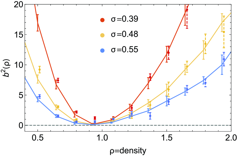
Refer to caption
Figure 9: Density bias squared measured in the simulation from the auto-correlation (dashed error bars) and cross-correlation (solid line and error bars) estimators given by equations (105) and (106) at different variances as labelled. Both approaches give consistent results.

Appendix E Asymptotic behaviour

The asymptotic behaviour of the density bias b(ρ^)𝑏^𝜌b({\hat{\rho}}) can be predicted by integrating equations (41) and (42) around the critical point which dominates the complex integration for ρ^^𝜌{\hat{\rho}} sufficiently large compared to ρcsubscript𝜌𝑐\rho_{c}. Bernardeau et al. (2015) indeed showed that in this regime, the cumulant generating function behaves like

φ(λ)=φc+(λλc)ρc+(λλc)3/2223π3(λλc)2π46π32+𝜑𝜆subscript𝜑𝑐𝜆subscript𝜆𝑐subscript𝜌𝑐superscript𝜆subscript𝜆𝑐32223subscript𝜋3superscript𝜆subscript𝜆𝑐2subscript𝜋46superscriptsubscript𝜋32\varphi(\lambda)=\varphi_{c}+(\lambda-\lambda_{c})\rho_{c}+(\lambda-\lambda_{c})^{3/2}\frac{2\sqrt{2}}{3\sqrt{\pi_{3}}}-(\lambda-\lambda_{c})^{2}\frac{\pi_{4}}{6\pi_{3}^{2}}+\cdots

with πi=Ψ(i)(ρc)subscript𝜋𝑖superscriptΨ𝑖subscript𝜌𝑐\pi_{i}=\Psi^{(i)}(\rho_{c}), the successive derivatives of the rate function at the critical point. This expansion for the cumulant generating function can be obtained by first inverting, around the critical point, the relation between ρ𝜌\rho and λ𝜆\lambda coming from equation (20)

λ=λc+i(ρρc)ii!πi+1,𝜆subscript𝜆𝑐subscript𝑖superscript𝜌subscript𝜌𝑐𝑖𝑖subscript𝜋𝑖1\lambda=\lambda_{c}+\sum_{i}\frac{\left(\rho-\rho_{c}\right)^{i}}{i!}\pi_{i+1}\,, (107)

which reads

ρ=ρc+2(λλc)π3π4(λλc)3π32+,𝜌subscript𝜌𝑐2𝜆subscript𝜆𝑐subscript𝜋3subscript𝜋4𝜆subscript𝜆𝑐3superscriptsubscript𝜋32\rho=\rho_{c}+\sqrt{\frac{2(\lambda-\lambda_{c})}{\pi_{3}}}-\frac{\pi_{4}(\lambda-\lambda_{c})}{3\pi_{3}^{2}}+\cdots,

and plugging the result into equation (19).

The large-density tail of the density PDF and density bias can then be derived by computing the inverse Laplace transform of the generating function φ(λ)𝜑𝜆\varphi(\lambda) when the integrand of equations (41) and (42) is dominated by its singular part, near λλc𝜆subscript𝜆𝑐\lambda\approx\lambda_{c}. In that case, Balian & Schaeffer (1989) and BPC showed that the dominant contribution of the path in the complex plane is along the real axis and wrapping around the singular value λcsubscript𝜆𝑐\lambda_{c} as illustrated on Fig. 10. As the two branches ++λc±iϵplus-or-minussubscriptsubscript𝜆𝑐iitalic-ϵ\mathbb{R}_{+}+\lambda_{c}\pm\hbox{i}\epsilon of that path yield complex conjugate contributions, the density PDF can be approximated by

P(ρ^){iϵ+λciϵ+dλπexp[φcλcρ^(λλc)(ρ^ρc)]×[1+223π3(λλc)3/2+]},𝑃^𝜌superscriptsubscriptiitalic-ϵsubscript𝜆𝑐iitalic-ϵd𝜆𝜋subscript𝜑𝑐subscript𝜆𝑐^𝜌𝜆subscript𝜆𝑐^𝜌subscript𝜌𝑐delimited-[]1223subscript𝜋3superscript𝜆subscript𝜆𝑐32P({\hat{\rho}})\approx\Im\!\left\{\!\int_{\hbox{i}\epsilon+\lambda_{c}}^{\hbox{i}\epsilon+\infty}\!\frac{\hbox{d}\lambda}{\pi}\!\exp[{\varphi_{c}\!-\!\lambda_{c}{\hat{\rho}}\!-\!(\lambda\!-\!\lambda_{c})({\hat{\rho}}\!-\!\rho_{c})}]\right.\\ \times\left.\left[1+\frac{2\sqrt{2}}{3\sqrt{\pi_{3}}}(\lambda\!-\!\lambda_{c})^{3/2}+\dots\right]\right\}\,, (108)

and the density bias by

b(ρ^)P(ρ^){iϵ+λciϵ+dλπexp[φcλcρ^(λλc)(ρ^ρc)]×[1+223π3(λλc)3/2+]bφ(λ)},𝑏^𝜌𝑃^𝜌superscriptsubscriptiitalic-ϵsubscript𝜆𝑐iitalic-ϵd𝜆𝜋subscript𝜑𝑐subscript𝜆𝑐^𝜌𝜆subscript𝜆𝑐^𝜌subscript𝜌𝑐delimited-[]1223subscript𝜋3superscript𝜆subscript𝜆𝑐32subscript𝑏𝜑𝜆\!\!b({\hat{\rho}})P({\hat{\rho}})\approx\Im\!\left\{\!\int_{\hbox{i}\epsilon+\lambda_{c}}^{\hbox{i}\epsilon+\infty}\!\frac{\hbox{d}\lambda}{\pi}\!\exp[{\varphi_{c}\!-\!\lambda_{c}{\hat{\rho}}\!-\!(\lambda\!-\!\lambda_{c})({\hat{\rho}}\!-\!\rho_{c})}]\right.\\ \times\left.\left[1+\frac{2\sqrt{2}}{3\sqrt{\pi_{3}}}(\lambda\!-\!\lambda_{c})^{3/2}+\dots\right]b_{\varphi}(\lambda)\right\}\,, (109)

where \Im is the imaginary part.

As already shown in Bernardeau et al. (2015), the resulting large-density PDF can then be written, to leading order, as

𝒫(ρ^ρc)=1πexp(φcλcρ^)[π2π3(ρ^ρc)5/2+],𝒫much-greater-than^𝜌subscript𝜌𝑐1𝜋subscript𝜑𝑐subscript𝜆𝑐^𝜌𝜋2subscript𝜋3superscript^𝜌subscript𝜌𝑐52{\cal P}({\hat{\rho}}\gg\rho_{c})\!=\!\frac{1}{\pi}\exp\left(\varphi_{c}-\lambda_{c}{\hat{\rho}}\right)\Im\!\left[\frac{\sqrt{\pi}}{\sqrt{2\pi_{3}}}({\hat{\rho}}-\rho_{c})^{-5/2}+\cdots\right]\,,

while the corresponding bias function is given to leading order as the ratio of equations (109) and (108)

b(ρ^ρc)=(ρ^ρc)V(1)(ρc)+V(ρc)π42π32V(2)(ρc)+12π3V(3)(ρc)+𝒪(1ρ^ρc)𝑏much-greater-than^𝜌subscript𝜌𝑐^𝜌subscript𝜌𝑐superscript𝑉1subscript𝜌𝑐𝑉subscript𝜌𝑐subscript𝜋42superscriptsubscript𝜋32superscript𝑉2subscript𝜌𝑐12subscript𝜋3superscript𝑉3subscript𝜌𝑐𝒪1^𝜌subscript𝜌𝑐b({\hat{\rho}}\gg\rho_{c})=({\hat{\rho}}-\rho_{c})V^{(1)}(\rho_{c})\\ \hskip 7.11317pt\!+\!V(\rho_{c})\!-\!\frac{\pi_{4}}{2\pi_{3}^{2}}V^{(2)}(\rho_{c})\!+\!\frac{1}{2\pi_{3}}V^{(3)}(\rho_{c})\!+\!{\cal O}\left(\!\frac{1}{{\hat{\rho}}-\rho_{c}}\!\right)\, (110)

where in the one-cell case V(ρ)=Ξijτj(ρjV(\rho)=\Xi_{ij}\tau_{j}(\rho_{j} is given by V(ρ)=ζ1(ρ)/σ2(Rρ1/3,Rρ1/3)𝑉𝜌superscript𝜁1𝜌superscript𝜎2𝑅superscript𝜌13𝑅superscript𝜌13V(\rho)=\zeta^{-1}(\rho)/\sigma^{2}(R\rho^{1/3},R\rho^{1/3}) and is nothing but the bias function V(ρ)=bφ(λ=Ψ(ρ))𝑉𝜌subscript𝑏𝜑𝜆superscriptΨ𝜌V(\rho)=b_{\varphi}(\lambda=\Psi^{\prime}(\rho)). In particular, one can compute the successive derivatives of V(ρ)𝑉𝜌V(\rho) at the critical density, for instance

V(1)(ρc)=(λcρc(ρc1/ν11/ν)+1νφc)ν(ρc1/ν1)2ρc11/ν.superscript𝑉1subscript𝜌𝑐subscript𝜆𝑐subscript𝜌𝑐superscriptsubscript𝜌𝑐1𝜈11𝜈1𝜈subscript𝜑𝑐𝜈superscriptsuperscriptsubscript𝜌𝑐1𝜈12superscriptsubscript𝜌𝑐11𝜈V^{(1)}(\rho_{c})=\frac{(\lambda_{c}\rho_{c}(\rho_{c}^{1/\nu}-1-1/\nu)+\frac{1}{\nu}\varphi_{c})}{\nu(\rho_{c}^{1/\nu}-1)^{2}\rho_{c}^{1-1/\nu}}\,. (111)
Refer to caption
Figure 10: The path line in the λ𝜆\lambda complex plane used for the computation of the large-density asymptotic forms follows a so-called Hankel contour.

Appendix F Approximation schemes for the slope

In the context of large-deviation theory, one can compute the rate function of the slope s=(ρ2ρ1)R1/ΔR𝑠subscript𝜌2subscript𝜌1subscript𝑅1Δ𝑅s=(\rho_{2}-\rho_{1})R_{1}/\Delta R by applying the so-called contraction principle which yields

Ψs(s^)=infρΨ(ρ,ρ+sΔRR1).subscriptΨ𝑠^𝑠subscriptinfimum𝜌Ψ𝜌𝜌𝑠Δ𝑅subscript𝑅1\Psi_{s}({\hat{s}})=\inf_{\rho}\Psi\left(\rho,\rho+s\frac{\Delta R}{R_{1}}\right)\,. (112)

The cumulant generating function of the slope can then be obtained through the Gartner-Ellis theorem as the Legendre transform of the rate function

φs(μ)=μsΨs(s)withμ=Ψs(s).formulae-sequencesubscript𝜑𝑠𝜇𝜇𝑠subscriptΨ𝑠𝑠with𝜇superscriptsubscriptΨ𝑠𝑠\varphi_{s}(\mu)=\mu s-\Psi_{s}(s)\quad{\textrm{with}}\quad\mu=\Psi_{s}^{\prime}(s)\,. (113)

The slope PDF then follows by Inverse Laplace transform as shown in equation (52)). It is now easy to see that the approximations of the slope PDF and bias can be obtained similarly to what has been done for the density. In this case, the slope cumulant generating function has typically two critical points sc<0superscriptsubscript𝑠𝑐0s_{c}^{-}<0 and sc+>0superscriptsubscript𝑠𝑐0s_{c}^{+}>0 corresponding to the zeros of the second derivative of the rate function d2Ψs(s)/ds2=0superscriptd2subscriptΨ𝑠𝑠dsuperscript𝑠20\hbox{d}^{2}\Psi_{s}(s)/\hbox{d}s^{2}=0.

For small slope sc<s<sc+superscriptsubscript𝑠𝑐𝑠superscriptsubscript𝑠𝑐s_{c}^{-}<s<s_{c}^{+}, the slope PDF and bias can be approximated by a saddle point approximation of equations (51) and (52) so that

𝒫(s^)Ψs′′(s^)2πexp(Ψs(s^)),𝒫^𝑠superscriptsubscriptΨ𝑠′′^𝑠2𝜋subscriptΨ𝑠^𝑠{\cal P}({\hat{s}})\approx\sqrt{\frac{\Psi_{s}^{\prime\prime}({\hat{s}})}{2\pi}}\exp\left(-\Psi_{s}({\hat{s}})\right)\,, (114)

and

b(s^)bφ(R1Ψs(s)/ΔR,R1Ψs(s)/ΔR).𝑏^𝑠subscript𝑏𝜑subscript𝑅1superscriptsubscriptΨ𝑠𝑠Δ𝑅subscript𝑅1superscriptsubscriptΨ𝑠𝑠Δ𝑅b({\hat{s}})\approx b_{\varphi}(-R_{1}\Psi_{s}^{\prime}(s)/\Delta R,R_{1}\Psi_{s}^{\prime}(s)/\Delta R)\,. (115)

However, this approximation is not sufficient (in particular it would predict b(0)=0𝑏00b(0)=0 which is far from the true value); one should Taylor expand the bias function bssubscript𝑏𝑠b_{s} around μ=Ψs(s^)𝜇superscriptsubscriptΨ𝑠^𝑠\mu=\Psi_{s}^{\prime}(\hat{s}) in order to get a better fit to the full numerical integration. This issue is left for future work.

Conversely, the asymptotes of the PDF and bias at large (positive and negative) slopes can be obtained similarly to what was done for the large-density regime (see appendix E). For instance, for large positive slope, the PDF can be approximated by

𝒫(s^sc+)=1πexp(φs(μc+)μc+s^)×[π2π3s,+(s^sc+)5/2]+𝒪((s^sc+)7/2)],{\cal P}({\hat{s}}\gg s_{c}^{+})\!=\!\frac{1}{\pi}\exp\left(\varphi_{s}(\mu_{c}^{+})-\mu_{c}^{+}{\hat{s}}\right)\\ \times\Im\!\left[\sqrt{\frac{{\pi}}{{2\pi^{s,+}_{3}}}}({\hat{s}}-s_{c}^{+})^{-5/2}]\right.\left.+{\cal O}\left(({\hat{s}}-s_{c}^{+})^{-7/2}\right)\right]\,, (116)

with πis+=Ψs(i)(sc+)superscriptsubscript𝜋𝑖limit-from𝑠superscriptsubscriptΨ𝑠𝑖superscriptsubscript𝑠𝑐\pi_{i}^{s+}=\Psi_{s}^{(i)}(s_{c}^{+}), while the corresponding slope bias is

b(s^sc+)=(s^sc+)Vs(1)(sc+)+Vs(sc+)π4s2(π3s)2Vs(2)(sc+)+12π3sVs(3)(sc+)+𝒪(1s^sc+),𝑏much-greater-than^𝑠superscriptsubscript𝑠𝑐^𝑠superscriptsubscript𝑠𝑐superscriptsubscript𝑉𝑠1superscriptsubscript𝑠𝑐subscript𝑉𝑠superscriptsubscript𝑠𝑐subscriptsuperscript𝜋𝑠42superscriptsubscriptsuperscript𝜋𝑠32superscriptsubscript𝑉𝑠2superscriptsubscript𝑠𝑐12subscriptsuperscript𝜋𝑠3superscriptsubscript𝑉𝑠3superscriptsubscript𝑠𝑐𝒪1^𝑠superscriptsubscript𝑠𝑐b({\hat{s}}\gg s_{c}^{+})=({\hat{s}}-s_{c}^{+})V_{s}^{(1)}(s_{c}^{+})\!+\!V_{s}(s_{c}^{+})\!-\!\frac{\pi^{s}_{4}}{2(\pi^{s}_{3})^{2}}V_{s}^{(2)}(s_{c}^{+})\!\\ +\!\frac{1}{2\pi^{s}_{3}}V_{s}^{(3)}(s_{c}^{+})\!+\!{\cal O}\left(\!\frac{1}{{\hat{s}}-s_{c}^{+}}\!\right)\,, (117)

where we define Vs(s)=bφ(R1Ψs(s)/ΔR,R1Ψs(s)/ΔR)subscript𝑉𝑠𝑠subscript𝑏𝜑subscript𝑅1superscriptsubscriptΨ𝑠𝑠Δ𝑅subscript𝑅1superscriptsubscriptΨ𝑠𝑠Δ𝑅V_{s}(s)=b_{\varphi}(-R_{1}\Psi_{s}^{\prime}(s)/\Delta R,R_{1}\Psi_{s}^{\prime}(s)/\Delta R).