Fermilab Lattice and MILC Collaborations
-mixing matrix elements from lattice QCD for the Standard Model and beyond
Abstract
We calculate—for the first time in three-flavor lattice QCD—the hadronic matrix elements of all five local operators that contribute to neutral - and -meson mixing in and beyond the Standard Model. We present a complete error budget for each matrix element and also provide the full set of correlations among the matrix elements. We also present the corresponding bag parameters and their correlations, as well as specific combinations of the mixing matrix elements that enter the expression for the neutral -meson width difference. We obtain the most precise determination to date of the SU(3)-breaking ratio , where the second error stems from the omission of charm sea quarks, while the first encompasses all other uncertainties. The threefold reduction in total uncertainty, relative to the 2013 Flavor Lattice Averaging Group results, tightens the constraint from mixing on the Cabibbo-Kobayashi-Maskawa (CKM) unitarity triangle. Our calculation employs gauge-field ensembles generated by the MILC Collaboration with four lattice spacings and pion masses close to the physical value. We use the asqtad-improved staggered action for the light valence quarks, and the Fermilab method for the bottom quark. We use heavy-light meson chiral perturbation theory modified to include lattice-spacing effects to extrapolate the five matrix elements to the physical point. We combine our results with experimental measurements of the neutral -meson oscillation frequencies to determine the CKM matrix elements , , and , which differ from CKM-unitarity expectations by about 2. These results and others from flavor-changing-neutral currents point towards an emerging tension between weak processes that are mediated at the loop and tree levels.
pacs:
12.15.Mm, 12.15.Hh, 14.40.Nd, 12.38.Gc 12.15.FfI Introduction
The search for new physics lies at the heart of high-energy physics research. Following the discovery of the Higgs boson at the Large Hadron Collider (LHC) in 2012, experiments at the LHC continue to search for new heavy particles which may be directly produced in high-energy collisions. Evidence for new physics, however, may also be found in indirect searches at low energies Hewett et al. (2012), where it would appear as a discrepancy between Standard-Model expectations and experimental measurements. Indirect searches can probe, and in some cases are already probing, new-physics scales that are orders of magnitude higher than those accessible through direct searches Isidori et al. (2010); Buras and Girrbach (2014); Buras et al. (2014a). Because we do not know a priori the properties (masses, couplings, quantum numbers) of the postulated new particles, indirect searches are being pursued across all areas of particle physics to provide as broad a search window as possible de Gouvea et al. (2013); Dawson et al. (2013); Butler et al. (2013); Albrecht et al. (2013). The central challenge with this approach is the high precision required from both theory and experiment to definitively interpret any deviations seen as evidence for new physics.
Neutral -meson () mixing is a particularly interesting process for indirect new-physics searches in the quark-flavor sector, since it is both loop and GIM suppressed in the Standard Model. The physical observables are the mass differences and decay-width differences between the heavy and light neutral -meson mass eigenstates, and the flavor-specific CP asymmetries . The -meson mass differences have been measured at the sub-percent level Amhis et al. (2014). The measured width differences and CP asymmetries have much larger uncertainties Amhis et al. (2014), but are expected to improve in the next several years Aaij et al. (2013a); Aushev et al. (2010).
Theoretical predictions of -mixing observables in both the Standard Model and beyond depend upon the hadronic matrix elements of local four-fermion operators in the effective weak Hamiltonian:
| (1) |
where is the renormalization scale. These operators arise after integrating out physics at energy scales above . Their matrix elements can be calculated in lattice QCD with standard methods. In the Standard Model, only one matrix element, , contributes to the mass difference . Beyond the Standard Model (BSM), however, can receive contributions from five distinct operators. These same five operators also contribute to the Standard-Model width difference .
In this paper, we calculate, for the first time in three-flavor lattice QCD, the matrix elements for all five local operators in the and systems. Only a few lattice-QCD results for -mixing matrix elements exist to-date Dalgic et al. (2007); Gámiz et al. (2009); Albertus et al. (2010); Bazavov et al. (2012a); Carrasco et al. (2014a); Aoki et al. (2015), with uncertainties of about 5–15% that are much larger than the corresponding experimental errors. Most efforts have focused only on the Standard-Model -mixing matrix elements Dalgic et al. (2007); Gámiz et al. (2009); Albertus et al. (2010); Aoki et al. (2015); Bazavov et al. (2012a). In Refs. Albertus et al. (2010); Aoki et al. (2015), the RBC and UKQCD collaborations treat the quark in the static limit Eichten and Hill (1990); Hasenfratz and Knechtli (2001); Della Morte et al. (2005), which results in errors. This effect is included in the error budget of Refs. Albertus et al. (2010); Aoki et al. (2015) via a power-counting estimate and contributes significantly to the total error. The HPQCD collaboration Dalgic et al. (2007); Gámiz et al. (2009); Dowdall et al. (2014) uses nonrelativistic QCD (NRQCD) for the -quark action Lepage et al. (1992); Gámiz et al. (2008). Their earlier calculations include three dynamical sea quarks Dalgic et al. (2007); Gámiz et al. (2009). Recently, however, they presented preliminary results Dowdall et al. (2014) (with perturbatively improved NRQCD Hammant et al. (2013)) from the first calculation of the Standard-Model -mixing matrix elements with four flavors of sea quarks (up, down, strange, and charm), where the average -quark mass is at its physical value Bazavov et al. (2010a, 2013). In Ref. Bazavov et al. (2012a), the Fermilab Lattice and MILC collaborations (Fermilab/MILC) presented a calculation of the ratio of -to- mixing matrix elements [ defined in Eq. (11)] using relativistic quarks with the Fermilab interpretation on a small subset of the three-flavor ensembles generated by the MILC collaboration Bernard et al. (2001); Aubin et al. (2004a); Bazavov et al. (2010b). The ETM collaboration Carrasco et al. (2014a) published the first results for the complete set of -mixing matrix elements, based, however, on gauge-field configurations with only two flavors of sea quarks. Preliminary results from this project have been reported earlier Bouchard et al. (2011); those results are superseded by this work.
Given theoretical calculations of the hadronic matrix elements, neutral -meson mixing can be used both to determine Standard-Model parameters and to search for new physics. In the Standard Model, the mass differences are proportional to the product of CKM matrix elements . Experimental measurements of can therefore be used to determine these CKM combinations, assuming no new-physics contributions. The ratio of CKM matrix elements can be obtained especially precisely from , because several correlated uncertainties in the - and -mixing hadronic matrix elements largely cancel. For Standard-Model tests, -mixing provides prominent constraints on the apex of the CKM unitarity triangle. For new-physics searches, it constrains BSM parameter spaces and in some cases enables discrimination between models. (For recent reviews, see, for example, Refs. Hansmann-Menzemer and Nierste (2015); Buras (2015); Buras et al. (2014a); Buras and Girrbach (2014); Nierste (2013); Lenz (2014); Bobeth (2014); Borissov et al. (2013) and for specific examples, see Refs. Blanke et al. (2015); Buras et al. (2014b, c); Buras and Girrbach (2013); Lenz et al. (2011, 2012); Brod et al. (2015); Bobeth et al. (2014a); Shimizu et al. (2013); Kim and Zurek (2014); Nelson and Scholtz (2015); Fortes et al. (2013); Dekens and Boer (2014); Queiroz et al. (2015); Arbey et al. (2015); Enomoto and Watanabe (2015).) Further, several small tensions are seen between experiment and theory for , , and the CP asymmetry Lunghi and Soni (2008); Buras and Guadagnoli (2008). All of the above comparisons are presently limited by the theoretical uncertainties on the hadronic matrix elements. To sharpen them and potentially reveal new-physics effects, better lattice calculations of the hadronic matrix elements that can leverage the impressive experimental precision are needed.
To that end, we improve upon the previous lattice -mixing matrix element calculations in several ways. We now compute the complete set of dimension-six four-fermion operators with three sea-quark flavors. We use the same valence- and sea-quark actions as in our earlier calculation of the ratio Bazavov et al. (2012a) but employ a much larger subset of the MILC configurations, including ensembles at four lattice spacings, covering a range of – fm. We quadruple the statistics on the ensembles used in Ref. Bazavov et al. (2012a), while adding ensembles at smaller lattice spacings and lighter sea-quark masses. Although the average -quark masses on the ensembles used in this work are all larger than in Nature, they extend down to , which corresponds to a pion mass MeV that is close to the physical value. Finally, we have changed the chiral-continuum extrapolation to account for certain effects that arise from the use of staggered light valence quarks Bernard (2013), thereby eliminating a significant source of systematic uncertainty in Ref. Bazavov et al. (2012a). These effects were discovered after a preliminary report Bouchard et al. (2011) on the current work appeared, so they were not included in the chiral extrapolations and error budget at that time. We now include this source of uncertainty, as well as all others. We present our matrix element results together with their correlations to facilitate their use in other phenomenological studies beyond this work. We also form several phenomenologically interesting combinations, including the SU(3)-breaking ratio and the corresponding bag parameters.
This paper is organized as follows. Section II presents the theoretical background and definitions of the hadronic matrix elements. Next, Sec. III provides details of the numerical simulations, including the gauge-field ensembles, the valence-quark actions, and the definitions of the two- and three-point lattice correlation functions. Section IV describes the fit functions and analysis procedures used to extract the desired matrix elements from the correlation functions. Section V summarizes the perturbative matching of the lattice matrix elements to the continuum, while Sec. VI describes how we correct a posteriori for small mistunings of the -quark masses. In Sec. VII, we extrapolate the matrix elements to the physical light-quark masses and to the continuum limit. Section VIII presents a detailed account of our systematic error analysis. Our final results are discussed in Sec. IX, where we also explore the implications of our results for Standard-Model phenomenology. Section X provides a summary and some outlook. The Appendices contain various details. In Appendix A, we tabulate our complete matrix-element and bag-parameter results for all operators, along with the correlations between them. In Appendix B, we describe in detail our methods for measuring the goodness of fits performed with Bayesian statistics. Appendix C provides equations for translating the one-loop chiral logarithm functions between the notation used in this work and in the original papers Detmold and Lin (2007); Bernard (2013).
II Theoretical background
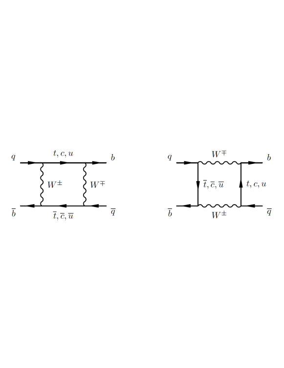
In the Standard Model, the leading-order electroweak interactions responsible for -meson mixing occur via the box diagrams depicted in Fig. 1.
The observables and are related to the off-diagonal elements of the time evolution matrix, and , as
| (2) |
up to corrections of order , while the observable is given by
| (3) |
where the CP violating phase . The mass and width differences provide complementary tests of the Standard Model. The mass differences are calculated from the dispersive part of the box diagram and are therefore sensitive to potential contributions from virtual heavy particles. On the other hand, the decay-width differences are obtained from the absorptive part, which predominantly receives contributions from light internal particles. Even so, new-physics contributions can affect the width differences.
The energy scale accessible in the loop of the box diagram in Fig. 1 is of order , and is far below the characteristic scale of the electroweak interactions, the -boson mass . Using the operator-product expansion (OPE) to treat this disparity of scales leads to a local effective four-quark operator description of mixing. For extensions of the Standard Model that involve interactions mediated by new heavy particles at the TeV scale or above, the local effective four-quark operator remains a convenient description. In this description, extending generically beyond the Standard Model, the effective Hamiltonian is
| (4) |
where the Wilson coefficients contain information specific to the short-distance physics associated with the flavor-changing interactions, and are the effective local four-quark operators. A basis of effective local four-quark operators is derived from the set of all Lorentz-invariant, color-singlet current-current interactions among heavy-light quark bilinears, reduced via discrete symmetries of QCD and Fierz rearrangement Hagelin et al. (1994); Gabbiani et al. (1996); Bagger et al. (1997), to
| (5a) | ||||
| (5b) | ||||
| (5c) | ||||
| (5d) | ||||
| (5e) | ||||
| (5f) | ||||
| (5g) | ||||
| (5h) | ||||
where and are continuum quark fields of given flavor, and are right- and left-handed projection operators , Greek indices denote color, and Dirac indices are implicit. The operators are the parity transforms of , . Because parity is a symmetry of QCD, the pseudoscalar-to-pseudoscalar matrix elements satisfy . Below, we exploit this identity to increase statistics.
The -mixing matrix elements have often been recast in terms of bag parameters , defined by Gabbiani et al. (1996)
| (6) | ||||
| (7) | ||||
| (8) |
where , , and . Before reliable calculations of the nonperturbative physics of the mixing matrix elements became available, the bag parameters were introduced, motivated by the so-called vacuum saturation approximation (VSA) Lee et al. (1973) where . Other conventions for the -parameters of the mixed-chirality operators are also used in the literature Lenz and Nierste (2007), for example in other recent lattice-QCD calculations Carrasco et al. (2014a); Dowdall et al. (2014). With the definitions in Eq. (8), however, and are indeed unity in the VSA.
The Standard-Model -meson oscillation frequency is often expressed in terms of the renormalization-group-invariant version of the bag parameter , as in Eq. (10) below. Following the notation of Ref. Aoki et al. (2014), we determine from (evaluated in the -NDR scheme), to two-loop order, by
| (9) |
where the coupling is defined in the scheme and and are the (scheme-independent) one- and two-loop beta-function coefficients. The one- and two-loop anomalous dimensions of are and , respectively; is scheme-independent, while is given in the -NDR scheme Buras et al. (1990).
In the Standard Model, only the matrix element contributes to the mass difference:
| (10) |
Here, the Inami-Lim function Inami and Lim (1981) describes the electroweak corrections and depends on the mass of the top quark in the loop of Fig. 1 through , while is the perturbative-QCD correction factor known at next-to-leading order Buras et al. (1990). For the Standard-Model decay-width difference Beneke et al. (1996); Lenz and Nierste (2007), as well as in general theories beyond the Standard Model, the mixing matrix elements (or equivalently bag parameters) of operators (–5) are also needed. Together, the five matrix elements (–5) are sufficient to parameterize the hadronic contributions to in all possible BSM scenarios, and therefore enable model-specific predictions related to mixing. More precise mixing matrix elements, of course, provide stronger new-physics constraints.
In the Standard Model, both and receive contributions from higher-dimensional operators beyond those in Eq. (5) that are not considered in this work. Corrections to the OPE used to derive Eq. (10) are negligible, because they are suppressed by . For , however, a second OPE, the so-called heavy-quark expansion Lenz and Nierste (2007), is needed to obtain a Standard-Model prediction in terms of local operators, yielding a joint power series in and . At leading order in the heavy-quark expansion, the Standard-Model expression for depends only on and either or . At , however, also receives contributions from the matrix elements . Further, at this order, matrix elements of dimension-seven operators not calculated in this work enter ; their contributions are numerically larger than those from the local matrix elements , and their uncertainties, after the reduction of errors on in this work, are the dominant source of error in the Standard-Model width differences Artuso et al. (2015).
Certain combinations of the hadronic matrix elements are especially useful for phenomenology. As discussed in the previous section, the theoretical uncertainties on are currently much larger than the experimental errors on , and therefore limit the precision with which one can obtain the CKM combinations . Many of the theoretical errors cancel, however, in the ratio , defined as
| (11) |
thereby enabling a determination of the CKM-element ratio from the corresponding ratio of mass differences:
| (12) |
that better leverages the experimental precision.
For Standard-Model calculations of the decay-width differences, it is useful to define the -suppressed combination Beneke et al. (1996)
| (13) |
The coefficient functions are known at next-to-leading order (NLO) in QCD Beneke et al. (1999) and are given in Eqs. (79)–(80) of Sec. IX. Because the leading contributions in the heavy-quark expansion cancel by construction in the combination in Eq. (13), the calculation of suffers from a larger uncertainty than for the individual matrix elements .
Finally, the decay-width differences are often parameterized in terms of the ratios of matrix elements (=2–5) because the theoretical uncertainties are reduced. These same ratios can also contribute to the mass differences in theories beyond the Standard Model. Hence they are useful for Standard-Model and BSM calculations of the ratio , as well as for predictions of -mixing observables in new-physics scenarios relative to their Standard-Model values.
III Lattice simulation
Here we summarize the details of the numerical simulations. First, in Sec. III.1, we describe the ensembles of gauge-field configurations and the light- and valence-quark actions employed in the analysis. Next, in Sec. III.2, we define the lattice two-point and three-point correlation functions used to obtain the desired -meson mixing matrix elements.
III.1 Gauge Configurations and Valence Actions
Our calculation employs gauge-field configurations generated by the MILC Collaboration with three dynamical sea quarks Bernard et al. (2001); Aubin et al. (2004a); Bazavov et al. (2010b). These ensembles use the Symanzik-improved gauge action Weisz (1983); Weisz and Wohlert (1984); Lüscher and Weisz (1985a, b) for the gluons and the asqtad-improved staggered action Blum et al. (1997); Orginos and Toussaint (1998); Lagaë and Sinclair (1998); Lepage (1999); Orginos et al. (1999); Bernard et al. (2000a) for the quarks. Generic discretization errors from the light-quark and gluon actions are of . In the numerical simulations, the fourth-root (square-root) of the strange-quark (light-quark) determinant is taken to reduce the number of staggered-fermion species from four to one (two) Hamber et al. (1983). Although this procedure violates unitarity and locality at nonzero lattice spacing Prelovsek (2006); Bernard (2006); Bernard et al. (2006, 2007); Aubin et al. (2008), a large body of numerical and theoretical evidence indicates that the desired continuum-QCD theory is obtained when the lattice spacing is taken to zero Adams (2005); Shamir (2005); Dürr (2006); Shamir (2007); Sharpe (2006); Bernard (2006); Bernard et al. (2008); Kronfeld (2007); Golterman (2008); Donald et al. (2011).
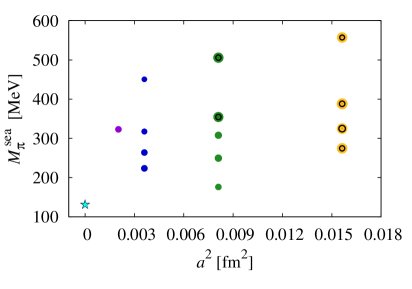
We analyze fourteen ensembles of gauge-field configurations with a range of pion masses and lattice spacings. Table 1 provides details of the numerical simulation parameters. On each ensemble, the two light sea-quark masses are set equal. The smallest simulated pion mass is 177 MeV, so only a short extrapolation to the value in Nature is required. For all ensembles, the strange sea-quark mass is tuned close to its physical value. We analyze four lattice spacings ranging from – fm to guide the continuum extrapolation. The spatial lattice volumes are sufficiently large ( for all ensembles, where is the lattice spatial extent) that finite-volume errors are expected to be at the sub-percent level for heavy-light-meson matrix elements; we nevertheless include these effects in our systematic error analysis. All ensembles have more than 500 configurations, and several contain as many as 2000. Figure 2 visually summarizes the range of pion masses, lattice spacings, and the statistical sample sizes.
| (fm) | (MeV) | (MeV) | |||||
| 0.12 | 0.02/0.05 | 2.8211(28) | 555 | 670 | 6.2 | 2052 | |
| 0.12 | 0.01/0.05 | 2.7386(33) | 389 | 538 | 4.5 | 2259 | |
| 0.12 | 0.007/0.05 | 2.7386(33) | 327 | 495 | 3.8 | 2110 | |
| 0.12 | 0.005/0.05 | 2.7386(33) | 277 | 464 | 3.8 | 2099 | |
| 0.09 | 0.0124/0.031 | 3.8577(32) | 494 | 549 | 5.8 | 1996 | |
| 0.09 | 0.0062/0.031 | 3.7887(34) | 354 | 415 | 4.1 | 1931 | |
| 0.09 | 0.00465/0.031 | 3.7716(34) | 306 | 375 | 4.1 | 984 | |
| 0.09 | 0.0031/0.031 | 3.7546(34) | 250 | 330 | 4.2 | 1015 | |
| 0.09 | 0.00155/0.031 | 3.7376(34) | 177 | 280 | 4.8 | 791 | |
| 0.06 | 0.0072/0.018 | 5.399(17) | 450 | 467 | 6.3 | 593 | |
| 0.06 | 0.0036/0.018 | 5.353(17) | 316 | 341 | 4.5 | 673 | |
| 0.06 | 0.0025/0.018 | 5.330(16) | 264 | 293 | 4.4 | 801 | |
| 0.06 | 0.0018/0.018 | 5.307(16) | 224 | 257 | 4.3 | 827 | |
| 0.045 | 0.0028/0.014 | 7.208(54) | 324 | 332 | 4.6 | 801 |
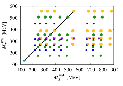
We also use the asqtad-improved staggered action for the light valence quarks. On each ensemble, we simulate with several values of the valence light-quark mass. These partially-quenched data are useful for constraining the fit coefficients in the chiral-continuum extrapolation in Sec. VII. For the quarks, we use the isotropic clover action Sheikholeslami and Wohlert (1985) with the Fermilab interpretation El-Khadra et al. (1997). We fix the clover coefficient to the tadpole-improved tree-level value , where is from the average plaquette. We tune the bare -quark mass, or, equivalently, the hopping parameter , such that the -meson mass agrees with the experimental value, following the general approach described in Ref. Bernard et al. (2011). For this work, we take the more recent and precise determinations of from Ref. Bailey et al. (2014). Table 2 provides details of the valence light- and -quark simulation parameters.
| (fm) | ||||||
|---|---|---|---|---|---|---|
| 0.12 | 0.02/0.05 | 1.525 | 0.0918 | 0.09439 | 4 | |
| 0.12 | 0.01/0.05 | {0.005, 0.007, 0.01, 0.02, | 1.531 | 0.0901 | 0.09334 | 4 |
| 0.12 | 0.007/0.05 | 0.03, 0.0349, 0.0415, 0.05} | 1.530 | 0.0901 | 0.09332 | 4 |
| 0.12 | 0.005/0.05 | 1.530 | 0.0901 | 0.09332 | 4 | |
| 0.09 | 0.0124/0.031 | 1.473 | 0.0982 | 0.09681 | 4 | |
| 0.09 | 0.0062/0.031 | {0.0031, 0.0047, 0.0062, | 1.476 | 0.0979 | 0.09677 | 4 |
| 0.09 | 0.00465/0.031 | 0.0093, 0.0124, 0.0261, 0.031} | 1.477 | 0.0977 | 0.09671 | 4 |
| 0.09 | 0.0031/0.031 | 1.478 | 0.0976 | 0.09669 | 4 | |
| 0.09 | 0.00155/0.031 | {0.00155, 0.0031, 0.0062, | 1.4784 | 0.0976 | 0.09669 | 4 |
| 0.0093, 0.0124, 0.0261, 0.031} | ||||||
| 0.06 | 0.0072/0.018 | 1.4276 | 0.1048 | 0.09636 | 4 | |
| 0.06 | 0.0036/0.018 | {0.0018, 0.0025, 0.0036, | 1.4287 | 0.1052 | 0.09631 | 8 |
| 0.06 | 0.0025/0.018 | 0.0054, 0.0072, 0.016, 0.0188} | 1.4293 | 0.1052 | 0.09633 | 4 |
| 0.06 | 0.0018/0.018 | 1.4298 | 0.1052 | 0.09635 | 4 | |
| 0.045 | 0.0028/0.014 | {0.0018, 0.0028, 0.004, | 1.3943 | 0.1143 | 0.08864 | 4 |
| 0.0056, 0.0084, 0.013, 0.16} |
The lattice temporal extents are sufficiently large that we can increase the statistics of our simulations by computing valence-quark propagators starting from multiple source locations on each configuration. In practice, we use four equally-spaced time sources on the majority of ensembles, with the exception of the fm, ensemble, where we use eight. We then average the results from all time sources on a single configuration. To reduce autocorrelations between measurements computed on configurations close in Monte-Carlo simulation time, we translate each gauge-field configuration by a random spatial shift before calculating valence-quark propagators. After applying this random shift, we do not observe any significant remaining autocorrelations, as confirmed by measurements of the autocorrelation time and simple binning studies shown in Sec. IV.
We convert lattice quantities to physical units using the scale , which is defined by the condition , where is the force between two static quarks Bernard et al. (2000b); Sommer (1994). The relative scale can be obtained precisely on each ensemble from the heavy-quark potential Bernard et al. (2000b); Bazavov et al. (2010b). To reduce the sensitivity of the lattice-spacing estimates to statistical fluctuations, we use values obtained from a fit of data on multiple ensembles to a smooth function of the coupling following Ref. Bazavov et al. (2010b). The explicit function employed is based on expectations from perturbation theory Allton (1996), and is given in Eqs. (115)–(116) of Ref. Bazavov et al. (2010b), where additional details on the smoothing procedure can be found. Here we use the updated mass-independent, smoothed determinations listed in Table 1. (The values are mass-independent because they have been extrapolated at fixed to physical quark masses from the simulated quark masses of each ensemble.) Compared with Ref. Bazavov et al. (2010b), the more recent analysis includes larger statistical samples for some ensembles, and omits ensembles with strange-sea quark masses much larger than the physical value. The fit uncertainties are below 1%, and are correlated between ensembles.
We multiply all lattice masses and matrix elements by the appropriate power of to make them dimensionless before proceeding to the chiral-continuum extrapolation and further error analysis. At the end we obtain results in physical units using Bazavov et al. (2012b)
| (14) |
fixed via the PDG Olive et al. (2014) value of . The quoted uncertainty takes into account the difference in values obtained by the MILC Bazavov et al. (2009) and HPQCD Davies et al. (2010) collaborations. Because the fit errors in Table 1 are smaller than the statistical uncertainties on the -mixing matrix elements, we do not include them in our central analysis. We estimate the systematic errors due to both the relative scale , including correlations between ensembles due to the smoothing procedure, and absolute scale in Sec. VIII, and add them to the chiral-continuum-fit error a posteriori.
III.2 Lattice Operators and Correlation Functions
We construct the two- and three-point correlation functions needed to obtain the matrix elements for neutral - and -meson mixing using the same methods as in our earlier calculation of the SU(3)-breaking ratio Bazavov et al. (2012a). In particular, we calculate them in a computationally efficient manner using the “open-meson propagators” described in Ref. Bazavov et al. (2012a), which are general objects with free spin and color indices. The three-point correlation functions needed for all five operators can be obtained from the combination of two open-meson propagators contracted with the appropriate Dirac structures. The needed two-point correlation functions can be obtained from a single open-meson propagator.
Starting with the light -flavored staggered field , we construct the naive field as in Refs. Bernard (2013); Wingate et al. (2003):
| (15) |
where , and the underlined field denotes four copies of the staggered field, with the (suppressed) “copy” index contracted with the right Dirac index of . To reduce heavy-quark discretization effects, we rotate the -quark field via El-Khadra et al. (1997)
| (16) |
where is a nearest-neighbor covariant distance operator. The coefficient is set to its value in tree-level tadpole-improved perturbation theory; Table 2 gives the numerical values used in our simulations.
In analogy with Eqs. (5), the lattice versions of the local four-quark operators are constructed from the rotated -quark field and the naive -flavored fields defined above:
| (17a) | ||||
| (17b) | ||||
| (17c) | ||||
| (17d) | ||||
| (17e) | ||||
and similarly for (). Again, and are color indices. With this choice, the leading discretization errors from the four-fermion operator are of order and Bazavov et al. (2012a); El-Khadra et al. (2016); Bernard (2013).
The continuum limit of the lattice four-quark operators in Eqs. (17) is complicated by the spin and taste components of the light quarks being “staggered” over a hypercube Kawamoto and Smit (1981); Sharatchandra et al. (1981); Gliozzi (1982); Kluberg-Stern et al. (1983), whereas all fields in Eqs. (17) reside at the same site. In the Symanzik effective field theory for staggered fermions Lee and Sharpe (1999), the operators take the form Bernard (2013)
| (18) |
where runs over all 16 Dirac matrices, and are taste indices, and and are copy indices. The fields on the left-hand side of Eq. (18) are those in the lattice simulation, while those on the right-hand side are defined in the continuum Symanzik (1983); the symbol can be read “has the same matrix elements as.” Compared with the continuum operators , the operators on the right-hand side of Eq. (18) have extra species indices (taste and copy) in addition to flavor.
On the right-hand side of Eq. (18), the opposite-parity contribution is familiar from heavy-light bilinears Wingate et al. (2003) and can be removed during the correlator fits, as discussed in Sec. IV. In the sum given explicitly, only the terms with and return the Dirac structure of the left-hand side. Following Ref. Bernard (2013), we refer to the others as “wrong-spin operators.” Because the and form a complete set, the same list of eight operators appears (with extra species indices) after carrying out the sum in Eq. (18), and the wrong-spin terms do not contain any new Dirac structures.
The -meson interpolating operators are similarly constructed from the fields and :
| (19) |
which creates (annihilates) a () meson. The spatial smearing function to the -quark propagator is given by the ground-state 1S wavefunction of the Richardson potential Richardson (1979); Menscher (2005). It provides good overlap of the interpolating operator with the -meson ground-state and suppresses unwanted contamination from excited states. Further details on the smearing are given in Ref. Bazavov et al. (2012b). In analogy with Eq. (18), the interpolating operator becomes
| (20) |
in the Symanzik effective theory after disentangling spin and taste.
The matrix elements can be extracted from three-point correlation functions with zero spatial momentum:
| (21) |
Despite the wrong-spin operators, the correlation function in Eq. (21) is dominated by contributions with the intended Dirac structure Bernard (2013). In the Symanzik-effective-theory notation, the three-point correlation function contains four terms of the form
| (22) |
where are taste indices, is the heavy-quark propagator, and the trace is over color and spin. When , the desired operator is recovered. The other terms arise only when a hard taste-changing gluon with some momentum components near is exchanged from one staggered-quark line to the other. In the Symanzik effective field theory, this effect is described by a four-quark interaction (among light quarks). These contributions are, thus, suppressed by a power of . Like any taste-violating effect, the terms lead to nonanalytic behavior in the chiral limit that can be described in staggered PT Bernard (2013). As discussed in Sec. VII, we can therefore account for them as part of the combined chiral-continuum extrapolation.
Figure 3 shows the structure of .

The local four-fermion operator is placed at a fixed location , where runs over the time sources, while the mesons are placed at all possible spacetime points and . In practice, we construct the three-point correlators from two open-meson propagators, corresponding to the and mesons at and , respectively, combining the free spin and color indices at as dictated by the spin-color structure of each operator . Because we average data from multiple time sources at the outset of the analysis, we henceforth drop the label in the three-point correlator and in the analogous two-point correlator (Eq. (23), below). The three-point correlator is now just a function of and .
To isolate the mixing matrix elements from , we need to remove the overlap of the -meson operator with the ground state. We obtain this normalization factor from the pseudoscalar two-point correlation function with zero spatial momentum:
| (23) |
which is constructed by tying together the open end of an open-meson propagator per Eq. (19).
Finally, to reduce statistical uncertainties, we average over sets of physically equivalent, but not numerically identical, data. The periodic temporal boundary conditions of the lattice ensure that, in the limit of infinite statistics, the two-point correlation functions are symmetric about the origin. We therefore average the two-point correlator values and as well as the three-point correlator values and . Further, parity conservation of QCD ensures that, in the limit of infinite statistics, the matrix elements are the same as . We therefore calculate both and and average them to improve the statistics. Additional details on these issues can be found in Ref. Bouchard (2011).
IV Correlator analysis
Here we discuss our determinations of the -mixing matrix elements from the two- and three-point correlation functions defined in Eqs. (21) and (23) of the previous subsection. In this section, dimensionful quantities are given in units of the lattice spacing, where the explicit factors of are suppressed to simplify expressions.
IV.1 Method
We estimate statistical uncertainties in the correlator analysis, and subsequently propagate them to the chiral-continuum extrapolation, via bootstrap resampling. In practice, on each ensemble we generate 600 bootstrap resamples; increasing the number does not change the estimated statistical errors in the two- and three-point correlation functions. We use the bootstrap distributions obtained from the two- and three-point fits to propagate the statistical errors cleanly from the correlator fits to the chiral-continuum extrapolation discussed in Sec. VII.
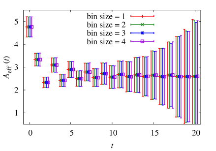
Before any fitting, we study the two-point correlation functions to assess the degree of autocorrelation between successive configurations in the Monte-Carlo evolution. We do this in several ways, each of which indicates that autocorrelations are negligible. First, we block the data with varying bin sizes. On all ensembles, we observe a negligible change in the errors of the correlator data when blocking is applied. This is illustrated in Fig. 4 which plots the effective amplitude [defined in Eq. (27)] of two-point functions on one of our coarsest ensembles and on our finest ensemble for different bin sizes.
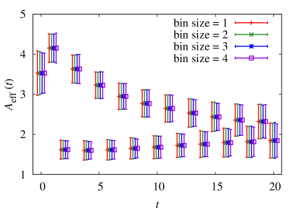
In addition, we calculate the autocorrelation coefficient for configuration separation , averaged over timeslices,
| (24) |
where . The exponential autocorrelation time is then obtained by comparing the calculated values of to the expected behavior, . We analyze the autocorrelations directly on the two-point data and separately on the principal component of the data covariance matrix. Both analyses yield , again indicating that no binning is required based on the criterion that a reasonable bin size is twice the autocorrelation time Montvay and Münster (1994). We therefore do not bin the correlator data in this work. Reference Bouchard (2011) provides further details on the autocorrelation studies.
We extract the hadronic matrix elements from simultaneous fits to two- and three-point correlation function data, constraining the fit parameters with Gaussian priors Lepage et al. (2002) whose central values are drawn randomly from the Gaussian distribution during bootstrap resampling. For all operators, ensembles, and valence-quark masses listed in Table 2, we fix the number of states included in the two- and three-point fit functions to be equal. We also use comparable fit intervals in physical units on all ensembles. We observe that the correlator fit results are stable against reasonable variations in the numbers of states and timeslices of data included in the fit. Details on the optimization of the correlation-function fits and determination of the -mixing matrix elements are given in the following subsections.
We implement the constrained fits in our analysis by minimizing the augmented defined in Eq. (121), which includes contributions from the priors. We employ the least-squares-fitting software package lsqfit Lepage (2012), which supports Bayesian priors and provides tools for correlated error propagation. We evaluate the relative quality of our correlator fits using a statistic denoted , which is defined in Eq. (122). Its definition is similar to the standard value Olive et al. (2014) but is based on the minimum of and a counting of the degrees of freedom suited to Bayesian analyses. By construction, lies in the interval . Larger values indicate greater compatibility between the data and fit function given the prior constraints. Unlike a value, however, is not expected to be uniformly distributed even when the hypothesis is correct. To test the influence of the priors on the best fit, we also examine a value based on the value of the standard function evaluated at the parameter values that minimize . Details and explicit formulas for and are provided in Appendix B.
IV.2 Two-point fits
We fit the -meson two-point correlator data to the functional form
| (25) |
where is the wavefunction normalization and is the temporal extent of the lattice. This fit function includes the effects of normal- ( even) and opposite-parity ( odd) states present in heavy-staggered meson correlation functions Wingate et al. (2003), and accounts for the contribution from backwards-propagating states associated with the use of periodic boundary conditions.
We loosely constrain the ground-state mass and amplitude using priors guided by the effective mass and amplitude defined as
| (26) | ||||
| (27) |
where in the exponent of Eq. (27) is chosen by eye based on the plot of in Eq (26), such that displays a plateau at large times. At each lattice spacing, we examine the effective mass and amplitude for all light sea- and valence-quark masses and choose common priors for and with widths large enough to cover the observed and . Figure 5 shows samples of and with the ground-state priors employed for all fits of two-point data at that lattice spacing.
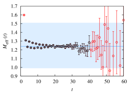
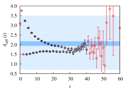
The prior widths are more than and larger than the uncertainties on the fitted ground-state energy and amplitude, respectively. We choose the priors for the lowest-lying oscillating state and the excited-state energy splittings guided by experimental measurements Olive et al. (2014) and quark-model predictions Di Pierro and Eichten (2001); Ebert et al. (2010). On all ensembles, we use priors that correspond to GeV, GeV, and GeV (). For the excited states (), we take the fit parameters to be the logarithms of the splittings between energy levels, . This automatically imposes the ordering .
We fit the two-point correlation functions using fit intervals , chosen for each ensemble based on the emergence of plateaus and the onset of noise in the effective mass and amplitude plots. We first vary with fixed , generally starting at and increasing it until excited-state contributions have significantly decreased. For example, for the correlation function shown in Fig. 5, we consider . The ground-state masses obtained from fits including earlier times have greater precision, but also greater contamination from excited states. We therefore include several pairs of excited and oscillating states in our fits to enable us to include early time slices. Initial studies showed that including six states was sufficient to accommodate excited-state contributions at early times, so we consider fits with . We also vary with fixed and find that fit results are insensitive to the addition of late-time-data for which statistical errors are larger. For the data shown in Fig. 5 we consider . We perform fits for all combinations of , , and within the ranges described here. Figure 6 demonstrates the stability of the fitted ground-state energy with respect to varying the number of states and timeslices included in the fit.
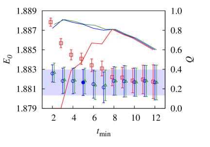
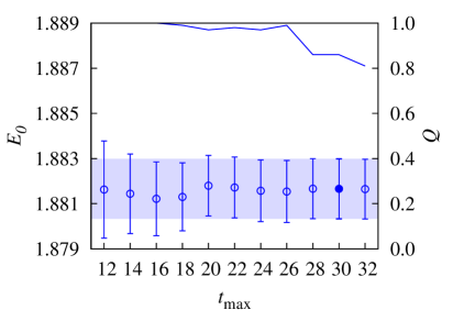
The two-point correlator data and fit results presented in Figs. 5 and 6 are representative of other valence-quark masses and sea-quark ensembles analyzed in this work.
Finally, after examining the stability plots for all light valence-quark masses and ensembles at a given lattice spacing, we select an optimal fit interval for each choice of , 4, and 6. We employ ranges for all two-point correlator fits that correspond to approximately the same physical distance on all lattice spacings. For each ensemble, we choose the same for all valence masses. The different ensembles have different numbers of configurations and, in some cases, different spatial volumes. As a result, the statistical precision of the data varies with ensemble. We therefore allow for a small variation of with ensemble at a given lattice spacing. In practice, differs between ensembles by no more than one timeslice. For , which is the number of states used in our central fit for the matrix elements, the fit intervals range from approximately at our coarsest lattice spacing to at our finest lattice spacing.
IV.3 Three-point fits
In analogy with Eq. (25), we fit the three-point correlator data to the functional form
| (28) |
where and are defined in Fig. 3. Because we combine the data from all time sources , from now on we set for simplicity. The desired hadronic matrix element , using notation introduced in Eq. (1) for the physical matrix element, is proportional to the ground-state amplitude as
| (29) |
where the factor of results from our use of nonrelativistic normalization of states in Eq. (28). The effect of periodic boundary conditions is negligible in the three-point data and is omitted from Eq. (28). As with the two-point correlation functions, we obtain loose priors for the ground-state amplitude by examining the effective amplitude, defined here to be
| (30) |
for all operators, ensembles and valence-quark masses on a given lattice spacing. Figure 7, left, shows an example three-point effective amplitude; plots for other operators, valence-quark masses and sea-quark ensembles look similar. Because the temporal oscillations from opposite-parity states are clearly visible in the three-point data, their contributions are easily identified in the correlator fits and can be removed to obtain the desired ground-state energy and amplitude.
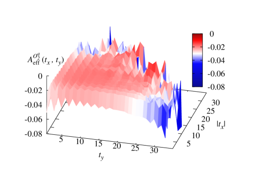
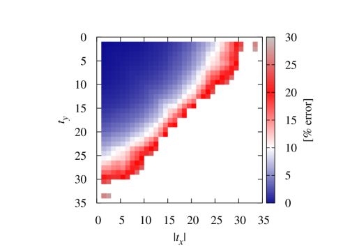
The three-point effective amplitudes display a plateau at moderately large and that has a magnitude of order . We choose a prior for the ground-state three-point amplitude of , consistent with the large widths used for the ground state in the two-point data.
The three-point correlators are functions of both the and timeslices, and , and we simultaneously fit the dependence on both times. Charge-conjugation symmetry ensures that the and mesons have identical energy eigenstates. The construction of the three-point correlation functions using open-meson propagators as described in Sec. III.2, in combination with the fact that the and correlators decay at the same rate, leads to an exact symmetry of the correlator data under the interchange . We choose the fit regions to reflect this symmetry, taking and and only including data for in the fit. These requirements define a class of fit contours in the - plane. We have verified that the fitted ground-state amplitudes are independent of the exact contour choice, however, as long as enough data are included.
We use slightly different fit regions for different operators. For the matrix elements , we use a triangular region in the - plane defined by
| (31) |
For the matrix elements , we use a fan-shaped region with
| (32) |
cutting out points at large and small times. The matrix element , which is extracted using both fit regions, provides a consistency check.
We perform simultaneous fits of the two- and three-point correlation functions using the same number of states for both, , and with common fit parameters for the energies and wave-function normalizations. For the two-point data, we use the optimal timeslices determined in Sec. IV.2. For the three-point data, we consider several fit ranges, , which are chosen based on inspection of the effective three-point amplitude and its relative error. For example, for the correlator data shown in Fig. 7, we examine the time ranges and . To select the preferred fit range and number of states, we first plot the fit results for the ground-state three-point amplitude vs for , 4, and 6. We find that leads to stable fits for all operators, light-quark masses, and ensembles and, therefore, choose this number of states as the basis for the rest of the analysis.
For each ensemble and operator, we choose so that it is roughly constant for all valence masses. As with in the two-point correlator analysis, we vary slightly among ensembles with the same lattice spacing. We also allow a small, monotonic increase in with increasing valence mass to accommodate an improving signal-to-noise ratio. Further, because the three-point data for different operators have different signal-to-noise ratios, we employ a slightly different for each operator. For a given lattice spacing and operator, the variation in between ensembles and valence mass is less than fm. The variation in the lowest time slice—when considering all operators, ensembles, and valence masses on a single lattice spacing—is slightly greater, but still less than fm. The minimum time slices included for the three-point correlator fits are similar on all lattice spacings, ranging from approximately 0.3–0.8 fm.
We then vary for the selected and to verify that the fitted ground-state three-point amplitude is insensitive to reasonable variations of , as shown in Fig. 8. We choose a value of that maximizes the amount of data in the fit without degrading the value. The result is an approximately equal number of data points in each fit. Consequently, ranges from at our coarsest lattice spacing to at our finest lattice spacing. Figures 7 and 8, and the choices inferred from inspecting them, represent well what we find for other ensembles and valence masses.
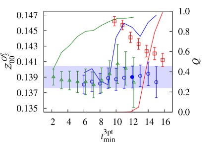
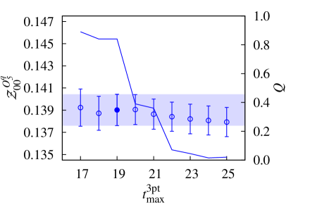
In addition to verifying that fit results are stable under reasonable changes to the number of states and time ranges in the fit, we perform several additional checks. We verify that ground-state energies obtained from the combined two- and three-point correlator fits are consistent with those from the two-point-only fits. We also ensure the fitted parameters are not in tension with the priors.


In total, we carry out 510 separate fits of the two- and three-point correlators for the five operators, fourteen ensembles, and seven or eight valence-light-quark masses per ensemble listed in Tables 1 and 2. As shown in Fig. 9, the distribution of values—defined in Appendix B—is approximately uniform, confirming that the chosen fit functions indeed describe our data. Further, it shows that the priors on the fit parameters and the slight variation in fit regions between operators, valence masses, and ensembles, have not introduced significant bias into our matrix-element results.
V Operator Renormalization and Matching
In this section we discuss the renormalization and matching needed to convert the bare lattice operators to renormalized operators evaluated at a common scale . When applied to the matrix elements obtained in the previous section, this procedure yields the corresponding renormalized matrix elements for every light-valence quark mass and lattice ensemble included in our analysis. The continuum matrix elements (evaluated at the physical light quark masses) are then determined in Sec. VII from a chiral-continuum extrapolation of the .
The four-fermion lattice operators defined in Eqs. (17) mix under renormalization. Like their continuum counterparts defined in Eqs. (5), they have nonzero anomalous dimensions. It is convenient to carry out the renormalization and matching to the desired continuum scheme in one step.
In dimensional regularization, the Dirac algebra does not close, and one has to specify a physical operator basis, distinct from the remaining “evanescent” operators Dugan and Grinstein (1991). The continuum one-loop renormalization coefficients have been calculated in the -NDR scheme for two different choices of evanescent operators Gámiz et al. (2008); Monahan et al. (2014). We denote by BBGLN the scheme defined in Refs. Beneke et al. (1999, 2002) and by BMU the scheme defined in Ref. Buras et al. (2000). These two schemes are the ones most widely used in the literature. These two choices of evanescent operators differ only in the renormalization of operators and . The lattice operators can be renormalized and matched to one of the schemes mentioned above by a suitable choice of dimension-7 operators and coefficient matrices Evans et al. (2009); El-Khadra et al. (2016):
| (33) |
where the bar denotes the chosen continuum scheme (e.g., -NDR-BBGLN), and is the renormalization scale. On the second line can be read “has the same matrix elements as,” as in Eq. (18). Using the rotated field in Eqs. (17) suffices to ensure that the coefficients start at order . We therefore neglect them in the matching process, leading to an uncertainty of order commensurate with that stemming from the choice of in the action. We estimate the effects of these corrections, together with other heavy-quark discretization errors, as explained in Section VII.1. When calculating the matching matrix , the quark/antiquark states select the same external tastes as do the -meson interpolating operators in the three-point correlation function, Eq. (21), and the loop integration automatically includes the hard taste-changing gluons. Further details of this matching procedure will be presented elsewhere El-Khadra et al. (2016).
In this paper, we carry out the renormalization and matching with perturbation theory, expanding
| (34) |
where the factor of and are normalization factors related to conventions for the staggered and clover fermion fields, respectively. Here the mass in is given by , where the critical hopping parameter is the value at which the rest mass vanishes. Only the one-loop coefficient in Eq. (34) is available at present El-Khadra et al. (2016).
From experience, we expect the coefficients to be large, because of contributions from external-leg tadpole diagrams Lepage and Mackenzie (1993). We use two modifications to Eq. (34) to improve convergence. One method is to absorb the large perturbative corrections into a redefinition of the basic parameters of the lattice action by dividing the gauge links in the action by a typical measure of the tadpole contributions via Lepage and Mackenzie (1993). The tadpole-improved renormalization is defined by:
| (35) | ||||
| (36) |
where we factor out for the asqtad quarks and , , for the heavy quarks. We call this the “tadpole-improved perturbative matching.” The values of and are calculated nonperturbatively on each ensemble and collected in Table 4. The one-loop tadpole-improved coefficients above are given by
| (37) |
where the one-loop value of is defined by For the fourth root of the plaquette, , while for the link in Landau gauge, ; here we examine tadpole improvement with both.
The other method is to factor out the renormalization associated with the vector currents El-Khadra et al. (2001); Harada et al. (2002), defining by
| (38) | ||||
| (39) |
and computing the matching factors and nonperturbatively. Then
| (40) |
where, perturbatively,
| (41) | ||||
| (42) |
Below we call the method based on Eq. (38) “mostly nonperturbative matching” (mNPR).
Table 3 gives the results El-Khadra et al. (2016) for and [which is the same for all , as is clear from Eqs. (37) and (40)] at the lattice spacings and bottom-quark masses employed in this work.
| (fm) | / | ||||||||||||
| 0.12 | 0.02/ | 0.05 | |||||||||||
| 0.01/ | 0.05 | ||||||||||||
| 0.01/ | 0.05 | ||||||||||||
| 0.01/ | 0.05 | ||||||||||||
| 0.007/ | 0.05 | ||||||||||||
| 0.005/ | 0.05 | ||||||||||||
| 0.09 | 0.0124/ | 0.031 | |||||||||||
| 0.0062/ | 0.031 | ||||||||||||
| 0.00465/ | 0.031 | ||||||||||||
| 0.0031/ | 0.031 | ||||||||||||
| 0.00155/ | 0.031 | ||||||||||||
| 0.06 | 0.0072/ | 0.018 | |||||||||||
| 0.0036/ | 0.018 | ||||||||||||
| 0.0025/ | 0.018 | ||||||||||||
| 0.0018/ | 0.018 | ||||||||||||
| 0.045 | 0.0028/ | 0.014 |
The values for in Table 3 are obtained using from the plaquette; the analogous factors using the Landau-link can be deduced from Eqs. (37) and (40) using the factors and tadpole-improvement factors in Table 4, and the values of and given above. The entries in Table 3 correspond to the BBGLN Beneke et al. (1999, 2002) choice of evanescent operators. To match to the BMU Buras et al. (2000) evanescent scheme, only a few entries change Bećirević et al. (2002); Monahan et al. (2014):
| (43a) | ||||
| (43b) | ||||
| (43c) | ||||
| (43d) | ||||
with the same changes for the corresponding (because no lattice diagrams enter in the difference between BBGLN and BMU).
When matching the lattice regulator to , the scale enters only via . We choose equal to the tree-level pole mass of the bottom quark, in lattice units, which is computed from the (dimensionless) quark-mass parameters of the lattice action. We need not, and do not, specify in physical units. In Sec. IX, however, we need to specify a scale to obtain several useful results and find , namely the mass, to be convenient. We do not distinguish between and the tree-level lattice pole mass, because the difference in the matching factor is of order .
For the strong coupling, we set , where is the renormalized coupling in the scheme Lepage and Mackenzie (1993) and is a typical gluon loop momentum in the process Lepage and Mackenzie (1993); Hornbostel et al. (2003). We use , the same choice made for heavy-light currents with the same actions and ensembles Bailey et al. (2014, 2015a, 2016). Other reasonable choices of would lead to differences of order , which are incorporated into the functional form for the chiral-continuum extrapolation, described in Sec. VII. The values of are obtained as in Ref. Mason et al. (2005) and are listed in Table 4.
| (fm) | ||||||||
| 0.12 | 0.02/0.05 | 0.0918 | 0.14073 | 0.8688 | 0.837 | 0.3047 | 0.4928(5) | 1.734(3) |
| 0.01/0.05 | 0.0901 | 0.14091 | 0.8677 | 0.835 | 0.3108 | 0.5031(5) | 1.729(3) | |
| 0.01/0.05 | 0.0860 | 0.14091 | 0.8677 | 0.835 | 0.3108 | 0.5266(6) | 1.729(3) | |
| 0.01/0.05 | 0.0820 | 0.14091 | 0.8677 | 0.835 | 0.3108 | 0.5494(6) | 1.729(3) | |
| 0.007/0.05 | 0.0901 | 0.14095 | 0.8678 | 0.836 | 0.3102 | 0.5030(5) | 1.730(3) | |
| 0.005/0.05 | 0.0901 | 0.14096 | 0.8678 | 0.836 | 0.3102 | 0.5030(5) | 1.729(3) | |
| 0.09 | 0.0124/0.031 | 0.0982 | 0.139052 | 0.8788 | – | 0.2582 | 0.4511(5) | 1.768(4) |
| 0.0062/0.031 | 0.0979 | 0.139119 | 0.8782 | 0.854 | 0.2607 | 0.4531(5) | 1.766(4) | |
| 0.00465/0.031 | 0.0977 | 0.139134 | 0.8781 | – | 0.2611 | 0.4543(5) | 1.766(4) | |
| 0.0031/0.031 | 0.0976 | 0.139173 | 0.8779 | – | 0.2619 | 0.4550(5) | 1.765(4) | |
| 0.00155/0.031 | 0.0976 | 0.139190 | 0.877805 | – | 0.2623 | 0.4550(5) | 1.765(4) | |
| 0.06 | 0.0072/0.018 | 0.1048 | 0.137582 | 0.8881 | – | 0.2238 | 0.4088(5) | 1.798(5) |
| 0.0036/0.018 | 0.1052 | 0.137632 | 0.88788 | – | 0.2245 | 0.4065(5) | 1.797(5) | |
| 0.0025/0.018 | 0.1052 | 0.137667 | 0.88776 | 0.869 | 0.2249 | 0.4066(5) | 1.797(5) | |
| 0.0018/0.018 | 0.1052 | 0.137678 | 0.88764 | 0.869 | 0.2253 | 0.4066(5) | 1.796(5) | |
| 0.045 | 0.0028/0.014 | 0.1143 | 0.136640 | 0.89511 | 0.8797 | 0.2013 | 0.3502(4) | 1.818(8) |
We define the flavor-conserving quantities and nonperturbatively through the standard charge-normalization conditions:
| (44) | ||||
| (45) |
The factors and are computed from two- and three-point functions, as discussed in Ref. Bazavov et al. (2012b), on the ensembles used in this work. The results are listed in Table 4. We use the same light-light renormalization factor for all light valence-quark masses (on the same ensemble) because its dependence on is very mild. At tree level, the product of these two factors is equal to in Eq. (35), since it is simply the combined normalization of the lattice fields.
The mostly nonperturbative method trades some pieces that contribute to the one-loop renormalization with corresponding nonperturbative pieces. In particular, the heavy- and light-quark wavefunction renormalizations cancel at one loop in the difference in Eq. (40), and they are instead included nonperturbatively in the matching relation Eq. (38) via the factors and . For operators , , and , the one-loop coefficients are generally smaller, but for and that is not the case. That said, the mNPR method is our preferred choice. In particular, on the finer lattices it works the best for , the matrix element with the strongest phenomenological motivation to achieve high precision.
VI Bottom-quark mass correction
As is customary with Wilson fermions, the Fermilab action uses the hopping parameter to parametrize the bare quark mass. We rely on the -tuning analysis discussed in detail in Ref. Bailey et al. (2014), which yielded the physical values for listed in Table 5.
In brief, low statistics runs were initially used to select the simulation values that were subsequently used in the full-statistics runs. After production running, the physical values were obtained by requiring the simulation -meson kinetic mass to match the PDG value.
| (fm) | |||
| 0.12 | 0.02/0.05 | 0.0879(9)(3) | 0.0221(50) |
| 0.12 | 0.01/0.05 | 0.0868(9)(3) | 0.0181(49) |
| 0.12 | 0.007/0.05 | 0.0868(9)(3) | 0.0181(49) |
| 0.12 | 0.005/0.05 | 0.0868(9)(3) | 0.0181(49) |
| 0.09 | 0.0124/0.031 | 0.0972(7)(3) | 0.0061(45) |
| 0.09 | 0.0062/0.031 | 0.0967(7)(3) | 0.0073(45) |
| 0.09 | 0.00465/0.031 | 0.0966(7)(3) | 0.0067(45) |
| 0.09 | 0.0031/0.031 | 0.0965(7)(3) | 0.0067(45) |
| 0.09 | 0.00155/0.031 | 0.0964(7)(3) | 0.0073(45) |
| 0.06 | 0.0072/0.018 | 0.1054(5)(2) | 0.0041(38) |
| 0.06 | 0.0036/0.018 | 0.1052(5)(2) | 0.0000(37) |
| 0.06 | 0.0025/0.018 | 0.1051(5)(2) | 0.0007(37) |
| 0.06 | 0.0018/0.018 | 0.1050(5)(2) | 0.0014(37) |
| 0.045 | 0.0028/0.014 | 0.1116(3)(2) | 0.0251(30) |
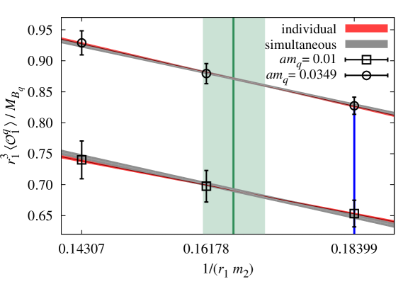
Here, we describe how we correct the matrix elements a posteriori to account for the fact that they were not computed at the physical . We simulate all five operators at three values of on the fm, ensemble. The three values include the simulation value and two others chosen to straddle the physical value. We obtain the bare lattice matrix elements as described in Sec. IV.3 for each of the three values, and at two values of the valence light-quark mass, and , which correspond roughly to the and mesons. We then convert the matrix elements to units using the values listed in Table 1 and match them to a continuum scheme via the mNPR method described in Sec. V. In the rest of the paper, we simply denote the renormalized lattice operators by , because their matrix elements differ from the continuum ones only by discretization and perturbative truncation errors that the systematic error estimate takes into account.
For each operator, we fit the data for using a function linear in the inverse tree-level kinetic quark mass, , to obtain the slope
| (46) |
with an accompanying uncertainty from the fit. This form is chosen because heavy-quark physics suggests a mild dependence on , which is identified with the inverse kinetic mass in the Fermilab interpretation. We try both separate fits for each set of valence light-quark data, and simultaneous fits to all data. Figure 10 shows these fits for .
For all operators, we find the slopes to be independent of . We therefore use -independent slopes from the simultaneous fits to determine the -correction for all valence-quark masses and ensembles. The slopes for each of the five operators are given in Table 6.
On each ensemble, we calculate the differences in inverse kinetic masses, , from the difference between the simulated and tuned values of , incorporating the uncertainties in and , as listed in Table 5. Finally, we obtain the needed corrections to the matrix elements from the product . The corrections are small, with relative shifts on the matrix elements of a few percent or less on the and 0.06 fm ensembles, and about 10% or less on the and 0.045 fm ensembles, where the differences between the tuned and simulation values are largest.
The way we incorporate the -quark mass corrections into the chiral-continuum fits is described in Sec. VII. Briefly, we include the shifts in the matrix elements as fit parameters constrained by priors with central values set to the calculated shift size and widths set to the computed errors. This approach allows us to propagate the uncertainties in our determinations of the slopes and in the physical values of directly into the chiral-continuum fit error.
| 1 | 2 | 3 | 4 | 5 | |||
|---|---|---|---|---|---|---|---|
| BMU | BBGLN | BMU | BBGLN | ||||
| 2.35(11) | 1.252(70) | 1.288(70) | 0.130(24) | 0.115(24) | 2.74(27) | 1.86(18) | |
VII Chiral-continuum extrapolation
We extrapolate the -mixing matrix elements to the physical light-quark masses and the continuum limit using SU(3), partially-quenched, heavy-meson, staggered chiral perturbation theory (HMrSPT) Aubin and Bernard (2006). The HMrSPT expressions for -mixing were derived in Ref. Bernard (2013) by generalizing the continuum calculation of Ref. Detmold and Lin (2007) to include the taste-symmetry-breaking effects of the staggered light quarks. References Detmold and Lin (2007); Bernard (2013) work to one loop in PT and use an effective Lagrangian for the meson derived at leading order in . As noted below, however, some effects of order are included in our chiral-continuum fit function, both explicitly and implicitly.
Every ensemble has a different lattice spacing, even those with the same nominal value (i.e., the “” listed in many tables). As explained in Sec. III, we multiply the matrix elements by the appropriate power of to bring them into dimensionless, but physical, units before performing the chiral-continuum extrapolation. The PT expressions require some external inputs, which we also bring into units with the value in Eq. (14).
Section VII.1 provides the expressions for the chiral fit function employed, both nonanalytic chiral logarithms and additional analytic terms, while Sec. VII.2 discusses specifics of the fixed inputs and priors used in the chiral fit. We will refer to this fit, which includes uncertainty contributions associated with the choice of fit function and inputs, as our base fit. The results of the base fit are given in Sec. VII.3. Below, in Sec. VIII, we study the stability of our fit results under reasonable modifications to the fit function and input data, showing that the errors quoted for the base fit include the uncertainties due to truncating the chiral and heavy-quark expansions and encompass the range suggested by the other cross checks.
VII.1 Chiral fit function
Schematically, the fit function for each matrix element takes the form
| (47) |
in which the individual terms are functions of the heavy and light meson masses, the lattice spacing, and the low-energy constants (LECs) of HMrSPT. The first term denotes the expression for the one-loop HMrSPT chiral logarithms, which contains nonanalytic dependence on the light-quark masses and lattice spacing. The next term, , represents analytic terms in the chiral expansion, namely, a polynomial in the light-quark masses and lattice spacing; this term is needed to cancel the scale dependence in . The remaining terms lie outside HMrSPT and parametrize other sources of systematic uncertainty. We account for heavy-quark discretization errors via and generic light-quark and gluon discretization errors of order via . The next term accounts for the uncertainty in the adjustment of the matrix elements from their values at the simulated heavy-quark mass to the physical . Finally, models neglected higher-order contributions to the operator renormalization, including off-diagonal terms in . Below, each of these terms is defined in detail.
VII.1.1 Chiral logarithms
The complete NLO HMrSPT expressions for the chiral logarithms are given in Ref. Bernard (2013). For matrix element ,
| (48) |
For ,
| (49) |
where and . Finally, for ,
| (50) |
where and, again, . In Eqs. (48)–(50), the coefficients and are the leading-order LECs for the matrix elements and , respectively, and they are the same as in the PT description of continuum QCD Detmold and Lin (2007). The terms , , and are standard contributions Detmold and Lin (2007) from wave-function renormalization, tadpole, and sunset diagrams, respectively. The terms and stem from tadpole and sunset diagrams of the wrong-spin operators discussed in Sec. III. Our notation for the wrong-spin terms in Eqs. (48)–(50) separates the LECs from the loop-diagram functions differently from Ref. Bernard (2013); Appendix C contains a dictionary to translate. Note that two additional LECs enter the one-loop expressions: the tadpole functions are proportional to , while the self-energy and sunset functions are proportional to , where is the pion decay constant and is the -- coupling.
The chiral logarithms depend on the ratio of the light pseudoscalar meson masses to the PT renormalization scale . At nonzero lattice spacing, taste-symmetry breaking splits the squared masses for mesons of different taste :
| (51) |
where and are the masses of constituents and , is the leading PT LEC, and () denote taste splittings Lee and Sharpe (1999). Taste violations also give rise to quark-disconnected hairpin diagrams at one loop in PT, whose contributions are suppressed by Aubin and Bernard (2003). The wrong-spin functions and are also of order after cancellations among several terms, each of which is of order unity.
We evaluate the loop-diagram functions with nonzero hyperfine and flavor splittings, and , in the propagators, as in Ref. Bazavov et al. (2012b) for -meson decay constants. We take the hyperfine splitting to be independent of the light valence flavor . We obtain the flavor splitting for arbitrary from the physical as follows. At lowest order in HMrSPT, the flavor splitting is proportional to the quark-mass difference:
| (52) |
where and are quark and meson masses, respectively. We then obtain the quantity from setting to and taking from the PDG Olive et al. (2014). The use of nonzero hyperfine and flavor splittings formally introduces contributions of order .
Our matrix-element data, of course, include contributions to all orders in the chiral expansion and in . We therefore choose not to impose heavy-quark spin-symmetry relations among the and in order to allow the fit parameters to absorb the renormalization parts of higher-order corrections. Because our data are all generated with a close-to-physical -quark, every parameter implicitly absorbs some dependence.
VII.1.2 Analytic terms in the chiral expansion
The analytic terms
| (53) |
are simple polynomials in the light-quark masses and lattice spacing. In practice, we use the dimensionless variables
| (54) |
and similarly for and , and
| (55) |
where
| (56) |
is the taste-averaged splitting, and each is the taste splitting defined via Eq. (51). The quantity is a convenient proxy for taste-breaking discretization effects. The NLO, next-to-next-to-leading order (NNLO), and next-to-next-to-next-to-leading order (N3LO) analytic expressions contain terms linear, quadratic, and cubic, respectively, in , , , and :
| (57) | ||||
| (58) | ||||
| (59) |
When these terms are expressed as polynomials in , , , and , the coefficients , , and are expected to be of order 1. The N3LO analytic terms are not included in our base fit, but are added to study the effect of truncating the chiral expansion, as discussed in Sec. VIII.1.4.
VII.1.3 Heavy- and light-quark discretization terms
We add the term to account for discretization errors in the -quark action and the four-quark operators. The HQET description of lattice gauge theory El-Khadra et al. (2016); Kronfeld (2000); Harada et al. (2002) gives for the leading terms
| (60) |
where each term has a different dominant lattice-spacing dependence:
| (61) | ||||
| (62) | ||||
| (63) |
The overall factors capture the typical size of the matrix elements , the functions describe the difference between lattice and continuum QCD Oktay and Kronfeld (2008), and the fit parameters and the powers of model HQET matrix elements. The explicit forms of the “mismatch” functions are given, for example, in Appendix A of Ref. Bazavov et al. (2012b).
When studying the stability of our fit results in Sec. VIII.1.5, we also consider the term
| (64) |
to account for generic discretization errors from the asqtad-improved staggered light-quark Lepage (1999) and Symanzik-improved gluon Lüscher and Weisz (1985b) actions. We do not, however, include in our base fit. This term is similar to the term in Eq. (57), which is proportional to instead of .
VII.1.4 Renormalization and correction
Before carrying out the chiral-continuum extrapolation, we renormalize the matrix elements with the mostly nonperturbative method described in Sec. V. Because the matching matrix in Eq. (38) is available only at one-loop order in perturbation theory, we incorporate renormalization effects of order and into the chiral-continuum fit by adding the terms
| (65) | ||||
| (66) |
summing over to incorporate higher-order perturbative mixing. The base fit allows to float and sets , but we also examine a fit with floating. When we carry out the matching with tadpole-improved perturbation theory—as a further estimate of truncation effects—we only consider .
Section VI describes how we determine the shift in the matrix elements between the simulated and physical -quark mass. We apply this correction by adding the term
| (67) |
to our fit function. While this term represents a correction to the data, both factors carry uncertainty. We therefore find it convenient to introduce the slopes (for each ) and the shifts in (for each ensemble) as fit parameters with Gaussian priors.
VII.2 Chiral fit inputs
In the base analysis used to obtain our final results, we fit all five matrix elements simultaneously because they share common parameters. Our base fit consists of the terms
| (68) |
and we require shared fit parameters to be equal for all five matrix elements. In the base fit, we employ the finite-volume expressions for the NLO logarithms, in which the one-loop integrals become discrete sums.
The parameters common to the expressions for all operators are , , , , , , in the chiral logarithms; the LECs for =1–5 and for =2–5; and . The parameters that are distinct for each operator are , , , in the PT analytic terms; , , , , , in the heavy-quark discretization terms; and in the generic light-quark and gluon discretization term. The indices of the higher-order renormalization parameters, and , make their dependence on the operators explicit. The -quark mass tuning term contains a slope for each operator and a difference for each ensemble.
Every parameter is constrained with a Gaussian prior Lepage et al. (2002). In Secs. VII.2.1 and VII.2.2, we explain the prior central values and widths used for each one. In addition, several inputs are fixed in our fits; we present their numerical values in Sec. VII.2.3. When converting lattice quantities to units, we multiply by the appropriate power of from Table 1, but treat the associated uncertainty outside the chiral-continuum fit, as discussed in Sec. VIII.2. On the other hand, when converting external, dimensionful quantities to units, we include the uncertainty in in Eq. (14) in the prior widths.
VII.2.1 Loosely constrained fit parameters
The most important parameters in the chiral-continuum extrapolation are constrained only loosely, to provide stability.
From our previous calculation of the SU(3)-breaking ratio with a smaller data sample Bazavov et al. (2012a), and from PT power-counting, we expect the LECs to be of order 1. For the leading LECs , we use priors for and . For the , which appear first at NLO, we use for (there is no ). Note that the prior widths on are two order of magnitude larger than the statistical errors on matrix elements obtained from the correlator fits.
As discussed in Sec. VII.1, the chiral analytic terms are written such that their coefficients , , and are expected to be of order 1 or smaller. For all of these coefficients, we take the prior central value to be zero. For the NLO coefficients, we use a prior width of 10 because we expect them to be well-determined by the data. For the NNLO and N3LO coefficients, we use a width of 1, guided by PT power-counting.
We take in the generic light-quark and gluon discretization term . The priors for the heavy-quark discretization terms are chosen as follows Bazavov et al. (2012b). By HQET power counting, we expect each parameter to be of order unity. Because we do not a priori know the signs, we take 0 for every prior central value. To choose the prior widths, we start by noting that each mismatch function is associated with a higher-dimension operator in HQET, although some operators share the same mismatch function. The width of each prior is chosen so that the width-squared equals the number of terms sharing the same mismatch function. Thus, the priors are 0(2) for , , and for , , for all –5. The four-fermion operators are subject to several dimension-seven corrections, denoted in Eq. (33). When the two Dirac matrices are the same, as they are for , there are five distinct ; when they are not, as for , there are ten Evans et al. (2009); El-Khadra et al. (2016). Therefore, we take , , and , .
For the unknown perturbative coefficients , we use priors 0(1). When terms of order are included, we again take priors .
VII.2.2 Constrained fit parameters
Other inputs to the chiral-continuum extrapolation are taken from experiment or from other lattice-QCD calculations. In each case, the prior central value and width are precisely those suggested by the external information.
In heavy-meson PT, the NLO chiral logarithms are multiplied by the pion decay constant and the -- coupling . Because the value of used in this paper is set from the PDG value of , we take
| (69) |
from the PT analysis of light pseudoscalar mesons Bazavov et al. (2009). For , we use unquenched lattice-QCD calculations Detmold et al. (2012a, b); Bernardoni et al. (2015); Flynn et al. (2016), taking
| (70) |
with an error covering the spread among the different results.
To choose a value for , we could consider the hyperfine splitting in the system, the system, or our lattice-QCD data. We showed earlier Bernard et al. (2011) that the asqtad ensembles reproduce the measured - hyperfine splitting, within lattice-QCD uncertainties. The experimental average for the hyperfine splitting for the system is more accurate than that for the system, although they are close to each other. Therefore, we choose the system, for which MeV Olive et al. (2014), or
| (71) |
including the error on .
The experimental value for the flavor splitting is MeV Olive et al. (2014). Plugging this number with Olive et al. (2014) and MeV Davies et al. (2010) into Eq. (52) gives , or
| (72) |
for the parameter that appears in the chiral fit function.
We take the hairpin parameters on the fm lattices to be and from chiral fits to light pseudoscalar-meson masses and decay constants on a subset of the MILC asqtad ensembles Aubin et al. (2004b). Because the hairpin contributions arise from taste-symmetry breaking, they are expected to scale with the lattice spacing in the same way as the taste splittings . Thus, to obtain values for the hairpin parameters at other lattice spacings, we scale them by the ratio of the weighted average of the taste splitting, Eq. (56), between the coarse and target lattice spacings.
VII.2.3 Fixed inputs
In our fits, we fixed the values of the leading-order, light-meson PT LECs () and in Eq. (51) because they can be obtained from the light pseudoscalar-meson spectrum with uncertainties negligible for the present purpose. The results from simple, linear fits in the valence-quark mass are given in Table 7.
| (fm) | |||||
|---|---|---|---|---|---|
| 0.12 | 0.2270 | 0.3661 | 0.4803 | 0.6008 | 6.832 |
| 0.09 | 0.0747 | 0.1238 | 0.1593 | 0.2207 | 6.639 |
| 0.06 | 0.0263 | 0.0430 | 0.0574 | 0.0704 | 6.487 |
| 0.045 | 0.0104 | 0.0170 | 0.0227 | 0.0278 | 6.417 |
We fix the two effective-field-theory cutoff scales, and , in the fits. We use MeV, based on studying the lattice-spacing dependence of matrix elements shifted to common light-quark masses via the chiral-continuum fit, and have explicitly checked that our fit results are insensitive to reasonable changes to its value. At a fixed order in PT, the chiral expression is independent of the scale that enters the chiral logarithms. We use GeV and have verified that the fit results change by less than one tenth of the fit error for and 0.75 GeV.
VII.3 Chiral fit results
Using the fit function in Eq. (68) and the inputs summarized in the previous section, we construct an augmented function,
| (73) |
where the multi-indices and run over all data for all (renormalized) operators, ensembles, and valence quark masses, and the run over all fit parameters discussed above. The data covariance is obtained from the bootstrap of the matrix elements, and the priors have been explained above. After finding the parameter set that minimizes , we extrapolate the renormalized matrix elements to the physical point by setting the light-quark masses to those in Table 8 and the lattice spacing to zero.
| 4.94(19) | 99.2(3.0) | 3.61(12) | 2.284(97) | 6.015 |
This procedure is repeated for alternative fits by modifying the fit function in Eq. (73). Figure 11 shows our base-fit results for each matrix element vs the squared meson mass , which is proportional to the light valence-quark mass. We obtain a correlated = 134.9/510.
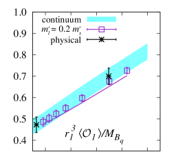
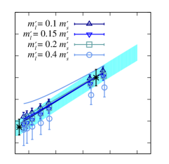
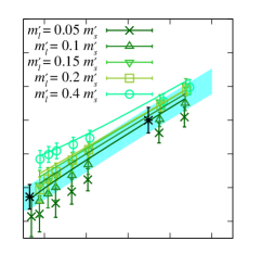
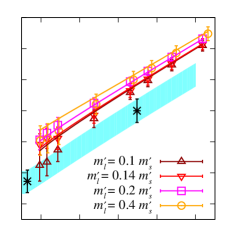
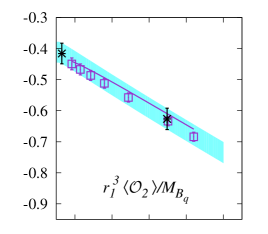
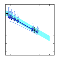
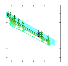
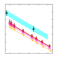
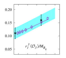
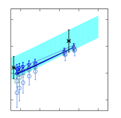
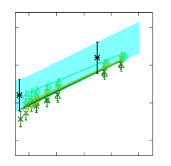
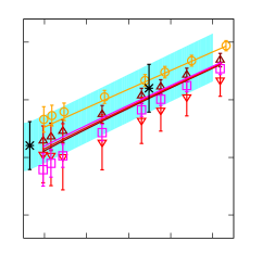
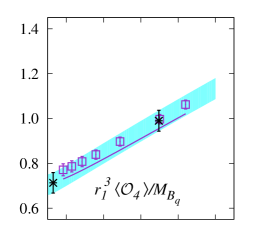
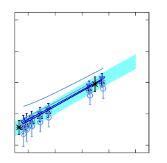
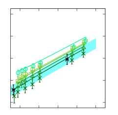
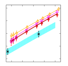
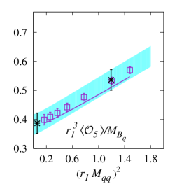
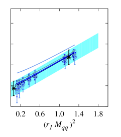
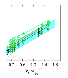
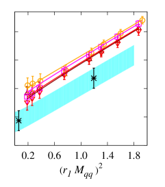
VIII Systematic Error Budget
We now consider all sources of uncertainty in our results and estimate their contributions to the total error. As discussed in the previous section, we perform a combined extrapolation to the physical light-quark mass and the continuum limit to extract the physical matrix elements from our lattice data. The chiral-continuum fit function of Eq. (68), used for our base fit, includes higher-order terms constrained with Gaussian priors. In Sec. VIII.1 we discuss systematic error contributions that are included in the chiral-continuum fit error, and the extensive tests we perform to check for residual truncation effects. Next, in Sec. VIII.2, we discuss the remaining contributions that are added to the chiral-continuum fit error a posteriori, with the exception of the error due to omitting charm sea quarks, which is considered separately in Sec. VIII.3. We also comment on the effect of correlations between the data, and compare the results of fits using various subsets of data. Last, in Sec. VIII.4, we summarize the sources of uncertainty considered and provide comprehensive error budgets for the matrix elements and .
In Secs. VIII.1 and VIII.2, we study the stability of our fit results and their relative goodness-of-fit, respectively, against reasonable variations of the fit function, input parameters and prior widths, and data included. We show stability plots only for the matrix elements and (), and for the ratio ; these plots are representative of the behavior observed for all matrix elements and ratios. We evaluate the relative fit quality using the augmented defined in Eq. (121), which includes contributions from the prior constraints on the fit parameters, and counts the number of prior constraints as additional data points when computing the degrees of freedom.
All of the fit variations used to test stability and estimate remaining systematic uncertainties employ the infinite-volume expressions for the chiral logarithms. As discussed in Sec. VIII.2.1, we find that finite-volume errors are negligible, which allows us to repeat the additional fits much more quickly without changing the conclusions about the errors.
VIII.1 Errors encompassed by the base chiral-continuum fit
As described in Sec. VII.2.2, we use Gaussian priors to constrain the fit parameters and most of the external inputs in our chiral-continuum fit. This allows for the uncertainties in the input parameters to be automatically included in the total fit error of the resulting matrix elements. Further, it enables the inclusion of higher-order terms in the chiral and heavy-quark expansions such that the fit error incorporates possible truncation errors. We track the error contributions of each data point and prior via the dependence of the best-fit parameters on each piece of information, including correlations among them, following the approach described in Appendix A of Ref. Bouchard et al. (2014). The statistical error is given by the quadrature sum of the errors from all data points. This procedure allows us to separate the total fit error () into approximate sub-errors. The sub-errors give a useful picture of the most (and least) important sources of uncertainty in the matrix elements and , but are not used in our final error budgets. Here we discuss the results of this estimated breakdown and also the fit variations that we perform to test the robustness of our error estimate. The stability of the central values and errors of our results under these fit variations, illustrated in Figs. 12–13, indicates that the corresponding uncertainties are indeed encompassed by the base-fit error.
Table 9 shows for each matrix element the approximate breakdown of the total fit error into the sub-errors. The first column shows the statistical error, which gives the largest contribution to the total fit error for all quantities listed.
VIII.1.1 Parametric inputs
The “inputs” column of the error budget in Table 9 shows the uncertainty contributions from all parametric inputs that are constrained by Gaussian priors. It includes the parameters , , , , , that appear in the chiral logarithms, Eqs. (48)–(50). It also includes the error on the physical - and -quark masses that are used in the chiral extrapolation (interpolation) of the matrix elements. The pion taste splittings , and the tree-level LEC are fixed; their errors are negligibly small and not included.
Although the error on the parameter is already included in our fit, one can study the dependence of our fit result on reasonable variations to the decay constant, which provides one measure of the uncertainty due to truncating the chiral expansion. For the base fit, we use the PDG value given in Eq. (69). To test the dependence of our result on reasonable variations of the decay constant, we perform a fit in which the decay constant is set to the PDG value Olive et al. (2014), or
| (74) |
The result of this fit is labeled “ vs. ” in Figs. 12–13. The largest observed change in central value is for the SU(3)-breaking ratio , which is still less than a half of .
VIII.1.2 Bottom-quark mass uncertainty
Section VI describes how we adjust the matrix elements calculated at the simulated -quark masses to the physical value. The uncertainty in this adjustment is included via priors on the difference between the simulated and tuned kinetic mass, , and on the slope, . The resulting error is given in the column labeled “ tuning” in Table 9.
VIII.1.3 Renormalization and matching uncertainty
The results of the base fit are obtained with matrix elements that are renormalized with the mNPR expression in Eq. (38) where the are calculated at one-loop order in perturbation theory as in Eq. (40). We take mNPR as our preferred approach because it includes all-orders and nonperturbative contributions from wave-function renormalization that are omitted with tadpole-improved perturbation theory. The chiral-continuum fit function for the base fit includes the generic terms of order in Eq. (65), where the unknown higher-order coefficients are constrained with Gaussian priors. The contribution to the error on each matrix element and from these terms is shown in the column labeled “matching” in Table 9.
We consider a number of fit variations to investigate the robustness of our error estimate and to test for residual effects of truncating the perturbative expansion in . First, we study the change in the matrix elements that results from varying the scale at which the strong coupling is evaluated in the range –, finding differences that are commensurate with the estimated matching errors in Table 9. Second, we remove the terms in Eq. (65) from the base fit function. Third, we include higher order corrections through , adding the terms in Eq. (66) to the base fit function. These two previous fits are labeled “mNPR” and “”, respectively, in Figs. 12–13. The changes in central values and error bars are negligibly small. Last, we perform two fits using the same fit function as for the base fit, but renormalize the matrix elements using tadpole-improved, one-loop perturbation theory taking two different definitions of in Eq. (35): the fourth root of the average plaquette and the average link in Landau gauge. These final fits are labeled “” and “”, respectively, in Figs. 12–13. Here we see more significant changes in the central values that are still within two . Notably, however, the variations between the “” and “” results indicate a systematic uncertainty associated with the choice of tadpole-improvement factor, bolstering our view that mNPR should be more reliable. Moreover, the stability of the mNPR results when adding terms of order and suggests that the errors on the renormalized matrix elements properly include the uncertainty from residual perturbative truncation effects.
VIII.1.4 Truncation of the chiral and heavy-meson expansions
We estimate the error due to the truncation of the chiral expansion from the contributions of the leading-order PT coefficients {, } and the LECs of all analytic terms that do not depend on the lattice spacing. This error is shown in the column labeled “chiral” in Table 9. We also investigate the size of residual truncation effects in both the chiral and the heavy-meson expansions through fit variations with fewer or additional terms; these are described below.
As discussed in Section VII.2, the chiral-continuum base fit includes all NLO and NNLO analytic terms of the chiral expansion. To test the robustness of our error estimate and check for the size of residual truncation effects, we consider two separate fit variations, the first including only NLO analytic terms, and the second including all analytic terms through N3LO. In the first case, where we omit the NNLO analytic terms, we also exclude the heaviest data points with , since they are above the expected range of validity of NLO PT. The results of this fit are labeled “NLO ” in Figs. 12–13. We observe only small changes to the results, but a relatively large change in the /dof due to the substantial alteration of both data set and fit function. The second case, where we include the complete set of N3LO analytic terms, yields the fit results that are labeled “N3LO” in Figs. 12–13. We observe negligible changes in both the central value and error bars. Comparing the result of the base fit with NNLO analytic terms to those from the fit variations with only NLO analytic terms and with analytic terms through N3LO, we conclude that our base fit correctly accounts for the error due to the truncation of the chiral expansion, and that residual truncation effects are negligibly small.
Finally, we study the impact on our fit of our choices for prior widths on the PT LECs, which are based on power-counting expectations. We perform three different fits in which we separately widen the priors by a factor of two on (1) the LO ( and ) parameters; (2) the NLO LECs (); or (3) the NNLO LECs (). These fits are labeled “LO 2”, “NLO 2”, and “NNLO 2”, respectively in Figs. 12–13. For all variations, we observe negligible changes with respect to the base fit. This confirms that our prior widths on the LECs are not unduly affecting our base-fit results.
As discussed in Section VII.1.1, we include in our base fit hyperfine- and flavor- splitting effects in the heavy-light mesons that appear in the PT loop integrals, which are the leading corrections in the expansion. To test for heavy-meson truncation effects, we set both splittings to zero. The result of this fit is labeled “no splitting” in Figs. 12–13. For this fit variation we see small-to-negligible changes in the matrix element results and in . Because the effects of the leading corrections included in the base fit are already so small, we conclude that residual heavy-meson truncation effects are negligible.
VIII.1.5 Light-quark discretization errors
Using the same procedure as for the “chiral” error, we estimate the uncertainty associated with light-quark discretization effects from the contributions of the PT LECs of all analytic terms that depend on the lattice spacing. This error is shown in the column labeled “LQ disc” in Table 9.
The base chiral-continuum fit function incorporates taste-symmetry breaking effects in the chiral logarithms, plus the corresponding taste-breaking analytic terms needed to maintain independence on the chiral scale. The base fit does not however, include a separate analytic term for generic discretization contributions from the light-quark and gluon actions. The results from a fit in which the generic discretization term [defined in Eq. (64)] is added to the base fit are labeled “generic ” in Figs. 12–13. We observe negligibly small changes in the central values and errors for the fitted matrix elements and for , and no discernible change in the /dof. This indicates that the analytic terms already included in the base-fit function are sufficient to describe the lattice-spacing dependence of the data, and that the base-fit error properly accounts for the contribution from light-quark discretization effects.
VIII.1.6 Heavy-quark discretization errors
We include six terms of order , , and in our base chiral-continuum fit to account for discretization effects from the heavy-quark action and four-quark operators. As in the previous sections, we estimate the error due to heavy-quark discretization effects from the contributions of the coefficients of these terms. This error is shown in the column labeled “HQ disc” in Table 9.
To test for residual heavy-quark discretization effects, we also perform alternate fits including fewer heavy-quark discretization terms. The results of these fits are shown in Figs. 12–13. Our first fit variation includes only the two terms. The results, which are labeled “HQ – only” show only small deviations from the base fit. For some matrix elements, the resulting errors are slightly smaller than for the base fit, indicating that additional terms are needed to saturate the error. Our second fit variation includes the two terms and the three at . Differences between the results of this fit, which are labeled “HQ – only”, and the base fit are imperceptible. Although including heavy-quark terms through already saturates the error from heavy-quark discretization effects, we include a sixth term of in the base fit because it appears formally at the same order in the heavy-quark expansion as the other five.
The heavy-quark discretization terms depend upon a cut-off scale , which is fixed in the chiral-continuum fit. Reasonable variations in this parameter are absorbed by changes in the fitted coefficients and therefore do not affect our results.
| statistics | inputs | tuning | matching | chiral | LQ disc | HQ disc | fit total | |
|---|---|---|---|---|---|---|---|---|
| 4.2 | 0.4 | 2.1 | 3.2 | 2.3 | 0.6 | 4.6 | 7.7 | |
| 4.6 | 0.3 | 1.1 | 3.7 | 2.6 | 0.6 | 4.6 | 8.0 | |
| 8.7 | 0.2 | 2.1 | 12.6 | 4.8 | 1.2 | 9.9 | 19.0 | |
| 3.7 | 0.4 | 1.7 | 2.2 | 1.9 | 0.5 | 3.9 | 6.4 | |
| 4.7 | 0.5 | 2.5 | 4.7 | 2.7 | 0.8 | 4.9 | 9.1 | |
| 2.9 | 0.4 | 1.5 | 2.1 | 1.6 | 0.4 | 3.2 | 5.4 | |
| 3.1 | 0.3 | 0.8 | 2.5 | 1.6 | 0.4 | 3.1 | 5.5 | |
| 5.9 | 0.3 | 1.4 | 8.6 | 3.0 | 0.7 | 6.9 | 13.0 | |
| 2.7 | 0.4 | 1.2 | 1.6 | 1.3 | 0.3 | 2.9 | 4.8 | |
| 3.4 | 0.4 | 1.8 | 3.4 | 1.9 | 0.5 | 3.6 | 6.7 | |
| 0.8 | 0.4 | 0.3 | 0.5 | 0.4 | 0.1 | 0.7 | 1.4 |
VIII.2 Errors considered after the base chiral-continuum fit
For some sources of uncertainty, we estimate the error contributions to the matrix elements and after the chiral-continuum extrapolation. To do so, we perform additional fits and compare the results to that of the base fit. This includes the errors from the relative scale and finite-volume effects. Further, although we include the indirect contributions of the error from the physical scale through its effects on physical input parameters in the chiral-continuum fit, here we consider its impact on the final conversion of the matrix elements from units to GeV. The error contributions from these uncertainty sources are listed in Table 11 and our methodology for their estimation is described below. We add these errors to the fit error a posteriori to obtain the “Total” error in Table 11.
VIII.2.1 Finite-volume effects
Our base fit employs the finite-volume expressions for the NLO chiral logarithms Bernard (2013), which are sums over the discrete momenta allowed with periodic boundary conditions. We estimate the error due to omitted higher-order finite-volume corrections by performing a second fit using the infinite-volume NLO chiral logarithms. We take half the shift in the central value between the base fit and the infinite-volume fit as an estimate of the finite-volume error. We expect this difference between NLO fits to be a conservative estimate of the finite-volume error, since the omitted finite-volume corrections are in fact of NNLO. The finite-volume error is listed in the “FV” column of Table 11, and is negligible when added in quadrature to the fit error.
VIII.2.2 Relative scale
We use the relative lattice spacings from Table 1 to convert our data from lattice units to units before adjusting for the -quark mass and performing the chiral-continuum fit. We must then account for the uncertainties in the values in our total error budgets for the matrix elements and .
We have considered including the values of as constrained parameters in the chiral-continuum fit in order to incorporate their uncertainties and correlations into the fit error. When we do so, we find that a fit that includes the errors on and their correlations (via Gaussian priors) returns fitted values on some ensembles outside of their prior constraints. We therefore fix the values of in our base fit to prevent the matrix-element data, which have much larger statistical errors than those for the heavy-quark potential, from significantly changing the relative lattice spacings. We take the increases in the errors on the matrix elements and from the fit in which we constrain the values with Gaussian priors as the errors due to uncertainties. To separate this error, we subtract in quadrature the base-fit error from the constrained--fit error. The resulting error estimate is shown in the column labeled “” in Table 11.
VIII.2.3 Absolute scale () uncertainty
We take the values for input meson masses and the pion decay constant in our chiral-continuum fit from the PDG. We constrain each of these parameters with Gaussian priors, and include the error from the conversion from GeV to units by adding the 0.7% error on the physical value of [Eq. (14)] to the PDG error to obtain the prior width. Similarly, the quark masses, which are also input parameters to the chiral-continuum fit function, are determined from experimentally measured meson masses, and are therefore also affected by the uncertainty in Eq. (14). As discussed in Sec. VIII.1.1, all of the indirect effects of the uncertainty on the error on the matrix elements and from the physical input parameters are already included in the chiral-continuum fit error.
After our chiral-continuum fit, however, we must still convert our final results for the matrix elements from units to GeV. This introduces an additional error due to the uncertainty in the physical value of which is listed in the column “” of Table 11. Note that this direct “” error does not enter dimensionless quantities such as the bag parameters and the ratios of matrix elements.
VIII.2.4 Isospin breaking and electromagnetism
We now consider the systematic effects on the mixing matrix elements and due to . With our partially quenched analysis we can vary the valence- and sea-quark masses independently. We obtain the physical - and -meson mixing matrix elements after the chiral-continuum fit by fixing the valence-quark masses to and given in Table 8, and fixing the light sea-quark mass to the average up-down quark mass . This accounts for the dominant isospin-breaking effects from the valence sector. Because the light sea-quark masses are degenerate in all our ensembles, however, the effects of isospin breaking in the sea are a source of systematic error in our calculation.
In order to estimate the error introduced by neglecting isospin-breaking effects in the sea we consider the dependence of the chiral-continuum fit function on the light sea-quark masses. Because the expressions for the -mixing matrix elements are symmetric under the interchange , the leading contributions from isospin-breaking in the sea sector are of , and are similar in size to NNLO terms in the chiral expansion. In practice, isospin-breaking errors arise from two types of terms in the chiral-continuum fit function: logarithms containing mixed valence-sea mesons, and analytic terms containing the sum of the squares of sea-quark masses. We estimate the numerical size of the errors in the matrix elements to be , where is the dimensionless PT expansion parameter defined in Eq. (54), and we have taken the coefficient to be unity based on power-counting expectations. Isospin-breaking errors in the ratio are expected to be further suppressed by the SU(3)-breaking factor . The error introduced by neglecting isospin breaking in the sea sector is negligible compared with the other sources of uncertainty discussed above, so it is not shown in Table 11.
The MILC asqtad gauge-field ensembles employed in this work do not include electromagnetism. This introduces errors of order from the omission of one-loop diagrams such as those with a photon connecting the valence and quarks, or a photon connecting one valence quark to a sea-quark loop.111In , further EM corrections stem from adding photons to the box diagrams. We estimate the numerical size of the omitted electromagnetic contributions to the matrix elements to be , where we include a loop-suppression factor of in the denominator. This is consistent with the size of the electromagnetic contribution to the proton-neutron mass difference, which has been found to be 2–3 MeV in QCD+QED simulations Borsanyi et al. (2015); Horsley et al. (2015). Again, errors in the SU(3)-breaking ratio are yet smaller. The error from omitting electromagnetism is shown in the “EM” column in Table 11.
Other recent dynamical lattice-QCD calculations of the -mixing matrix elements Gámiz et al. (2009); Carrasco et al. (2014a); Aoki et al. (2015) do not account for isospin breaking, which is currently a subleading source of error compared to other uncertainties. It is interesting, however, to estimate the size of the omitted valence isospin-breaking corrections to these results with our data. We do so by taking the difference between the matrix elements evaluated with the correct valence-quark mass and those with the valence-quark mass fixed to the isospin average, i.e.:
| (75) |
with the sea-quark mass set to the average light-quark mass in both. Table 10 gives the valence isospin-breaking corrections for all five matrix elements =1–5 and also for the ratio . The corrections to the matrix elements are positive, and are about a half a percent. They can in principle be used to adjust lattice results for -mixing matrix elements from isospin-symmetric full-QCD simulations, although in practice this is not yet necessary since the isospin-breaking shifts are much smaller than the total errors currently quoted. Nevertheless, they indicate that the inclusion of valence isospin breaking will be important once the errors on the -mixing matrix elements reach the few percent level.
Further, because the matrix elements are proportional to the square of the -meson decay constant, the valence isospin-breaking corrections in Table 10 can provide a very rough guide as to the size of the analogous shifts that might be expected for . If one assumes that valence isospin breaking is negligible in the bag parameters and takes the entire correction to the matrix elements to be from , the approximately 0.5% shifts in would correspond to about a 0.25% shift in , or about 2.5 MeV. Numerically, a correction of this size would be important given the uncertainties currently quoted on the most precise lattice -meson decay constant calculations Na et al. (2012); Dowdall et al. (2013), which are performed in isospin-symmetric full QCD. We will compute the valence isospin-breaking correction to (and ) directly in our forthcoming - and -meson decay-constant analysis Neil et al. (2015), which includes partially-quenched data.
| 1 | 2 | 3 | 4 | 5 | ||
|---|---|---|---|---|---|---|
| (%) | 0.51(11) | 0.56(12) | 0.49(15) | 0.423(93) | 0.409(99) |
VIII.2.5 Other consistency checks
We check the consistency between fit results with different data subsets by performing two additional fits in which we drop either the data on our largest or smallest lattice spacing. The results of these fits are labeled “no fm” and “no fm” in Figs. 12–13, respectively. As expected, the errors increase when data is omitted. In most cases, the new central values differ from those of the base fit by less than one , with one observed difference of almost 2 as would be expected given so many fits. The consistency between the fit results with different subsets of data is further evidence that our chiral-continuum fit provides a good description of the observed discretization effects.
Finally, to study the effect of correlations between the operators that mix under renormalization and due to the choice of local four-quark operators, we perform separate fits to the data for each operator. The results of these fits are labeled “individual” in Figs. 12–13 and are very close to those of the base fit. As expected, the errors on the individual fit results are larger because the contributions from the other off-diagonal matrix elements cannot be resolved, so their uncertainties are governed by the prior widths on the associated LECs (s).
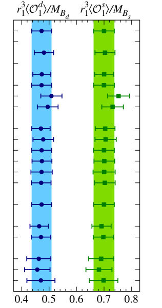
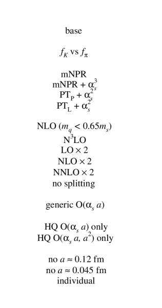
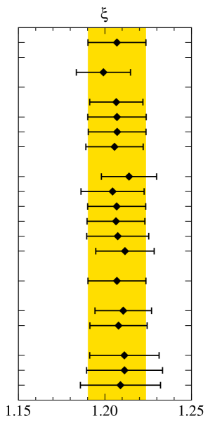
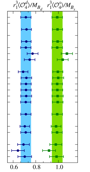


VIII.3 Omission of the charm sea
The MILC asqtad ensembles do not include charm sea quarks. One can expand the charm-quark determinant in powers of to obtain an estimate of the leading effects of this omission Nobes (2005). The first nonvanishing contribution is proportional to , which is absorbed into the bare gauge coupling. The next contribution—after using identities and eliminating the redundant operator —is . Thus, the ensembles lack a contribution of order . Taking GeV from the PDG Olive et al. (2014) and reasonable values for and leads to error estimates of 1%–2% for the matrix elements, which should be suppressed by in the SU(3)-breaking ratio .
To check this power-counting estimate, we have examined results for related matrix elements from calculations with different numbers of sea quarks. A comparison of four- and three-flavor results for kaon, -, and -meson decay constants Rosner et al. (2015); Aoki et al. (2014) yields differences that are consistent with zero within errors, but that could allow for effects as large as 1%–2%. There are also no significant differences between three- and two-flavor results Aoki et al. (2014), which one might expect to be larger, since contributions from the strange sea are entirely nonperturbative, unlike the charm sea case. In the kaon system, where lattice results with total errors at the sub-percent level exist for both the three- and four-flavor cases, the differences are much smaller than the sub-percent level errors.
The scale dependence of the -mixing matrix elements gives rise to another charm-loop effect that must be considered. Because we obtain the matrix elements at the scale , charm-loop contributions to the scale dependence of the matrix elements between and are omitted in a three-flavor calculation. We estimate this effect by taking our result for and evolving it to using the two-loop -function and anomalous dimension given in Eq. (9) evaluated with , and then evolving the matrix element back to with . This procedure yields a shift of .
In summary, it is possible that the effects on -mixing matrix elements from omitting charm sea quarks are as small as in the kaon system, i.e., at-or-below the sub-percent level. In the absence of similarly precise results in the - and -meson systems, however, we conservatively use the power counting estimate discussed above and assign an error of on the -mixing matrix elements from the omission of charm sea quarks. This estimate accounts for both effects of omitting charm-sea quarks considered here. For , we consider the additional SU(3) breaking suppression factor in our estimate, and assign a similarly conservative error of due to omitted charm-sea effects. The bag parameters are ratios of mixing matrix elements and decay constants, and we assume that the remaining contributions from charm loops are negligible compared to other uncertainties. Hence, we do not assign an error due to the omission of the charm sea to our bag parameter results. Finally, because the estimated charm sea error is much less quantitative than all our other uncertainties, we do not add it in quadrature to the total error. Instead we list it as a separate “charm sea” error in Table 11 and also show it separately in our results presented in Sec. IX.
VIII.4 Error summary
In this subsection we present a summary of all systematic errors in our lattice-QCD calculation, and then combine them to obtain the total errors in the matrix elements and . Our base chiral-continuum fit function includes higher-order terms constrained with Bayesian priors to account for the dominant sources of systematic error. As illustrated in Figs. 12–13, we consider over a dozen fit variations to study residual truncation effects for the dominant sources of uncertainty in our lattice calculation, including chiral extrapolation, light- and heavy-quark discretization, and renormalization effects. We conclude that the fit error from our base chiral-continuum fit properly accounts for these effects. Table 9 gives an approximate breakdown of the chiral-continuum fit error into separate contributions for each matrix element and the ratio as described in Sec. VIII.1. We then add in quadrature to the “fit total” error all the significant contributions that are not already included in the chiral-continuum fit uncertainty (i.e., those from finite-volume effects, uncertainties, the physical scale , and electromagnetic effects) to obtain the “Total” error in Table 11. Errors associated with isospin breaking are estimated to be negligible. In summary, the “Total” error of Table 11 includes all significant contributions to the matrix elements and after all possible sources of uncertainty have been considered with the exception of our estimate of dynamical charm effects (discussed in Sec. VIII.3), which is listed separately in the last column of the table. This separation will enable the errors on our results to be easily adjusted in the future if more reliable estimates of the size of charm sea-quark contributions become available.
| Fit total | FV | EM | Total | Charm sea | |||
|---|---|---|---|---|---|---|---|
| 7.7 | 0.2 | 2.5 | 2.1 | 0.2 | 8.3 | 2.0 | |
| 8.0 | 0.3 | 2.8 | 2.1 | 0.2 | 8.8 | 2.0 | |
| 19.0 | 2.5 | 2.1 | 0.2 | 19.3 | 2.0 | ||
| 6.4 | 2.1 | 2.1 | 0.2 | 7.1 | 2.0 | ||
| 9.1 | 2.2 | 2.1 | 0.2 | 9.6 | 2.0 | ||
| 5.4 | 0.1 | 1.9 | 2.1 | 0.2 | 6.1 | 2.0 | |
| 5.5 | 0.1 | 2.1 | 2.1 | 0.2 | 6.2 | 2.0 | |
| 13.0 | 1.9 | 2.1 | 0.2 | 13.3 | 2.0 | ||
| 4.8 | 1.7 | 2.1 | 0.2 | 5.5 | 2.0 | ||
| 6.7 | 1.8 | 2.1 | 0.2 | 7.2 | 2.0 | ||
| 1.4 | 0.6 | 0 | 0.04 | 1.5 | 0.5 |
IX Results
Here we present our final results with total uncertainties that include all contributions to the errors considered in the preceding section. As discussed there, we report the charm-sea error separately from the total of the statistical and all other systematic uncertainties. First, in Sec. IX.1, we give the -mixing matrix elements. Next, in Sec. IX.2, we provide quantities that are derived from the -mixing matrix elements, such as the SU(3)-breaking ratio and the bag parameters . In both Secs. IX.1 and IX.2, we highlight a few main results—such as for the renormalization-group-invariant quantities for the Standard-Model operator —and compare our results with those from other calculations. Appendix A provides our complete results for all matrix elements and bag parameters, including their correlations. Finally, in Sec. IX.3 we use the -mixing matrix elements and combinations thereof to compute phenomenologically-interesting observables and CKM matrix elements within the Standard Model.
The tables in Appendix A present the matrix elements and bag parameters for operators () corresponding to both the BMU and BBGLN evanescent-operator schemes discussed in Sec. V. These results are obtained from separate chiral-continuum fits which employ different matching coefficients for . Although the matching coefficients for are identical in the two schemes, the fitted matrix elements can differ slightly due to correlations with . In practice, the results for differ by at most 1 in the least significant digit reported. We therefore present results for and the corresponding bag parameters from only the BBGLN fit.
IX.1 Matrix elements
We convert our final results for the -mixing matrix elements (; =1–5), obtained in the -NDR scheme, to the combination via Eqs. (6)–(8), taking the quark masses in Eqs. (7) and (8) from Table 12. Here, and in the rest of the paper, we choose GeV. Our final results for are listed in Table 13 of Appendix A. They are the complete set needed to describe neutral -meson mixing in the Standard Model and all extensions thereof. To facilitate their use in other phenomenological analyses, we provide the matrix of correlations between their values in Table 14.
Figure 14 compares our results for the full set of -mixing matrix elements with those of the ETM collaboration Carrasco et al. (2014a), which were obtained using two sea-quark flavors. Our matrix-element errors range from about 5–15%, and are larger for operators due to the need to extrapolate to the physical -quark mass. The uncertainties quoted by ETM are similar, but do not include an uncertainty due to omitting the strange sea quark in their error budget. Our results for agree with those of ETM, while those for differ by about 2.
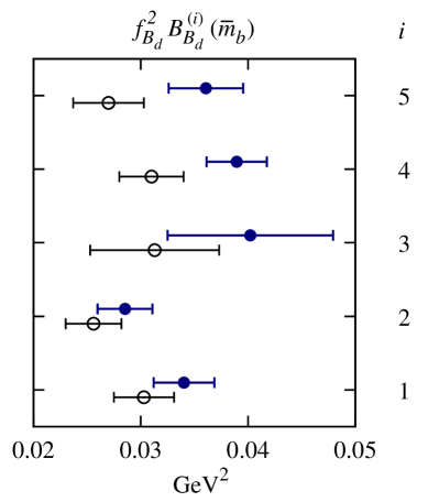
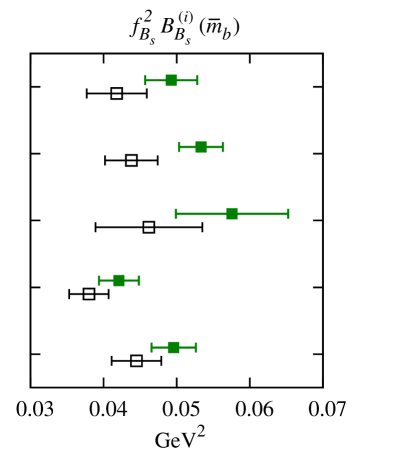
It is common to express the Standard-Model oscillation frequency in terms of the renormalization-group-invariant (RGI) combination , which is related to at two loops by Eq. (9). Taking from Table 12, we obtain
| (76) | |||||
| (77) |
where the first error is from the column labeled “Total” in Table 11 and the second is our estimated error from the omission of charm sea quarks.222The first error also includes a 0.2% uncertainty estimate for converting from -NDR to RGI. As shown in Fig. 15, left, our results in Eqs. (76) and (77) agree with those from previous unquenched lattice-QCD calculations, but have smaller uncertainties. Compared with the other three-flavor calculations by the HPQCD Gámiz et al. (2009) and RBC/UKQCD collaborations Aoki et al. (2015), our data set includes lighter pions and finer lattice spacings. The RBC/UKQCD errors are dominated by their estimate of the neglected contributions of order due to their use of the static approximation. We note that the HPQCD results Gámiz et al. (2009) and the preliminary matrix elements from Fermilab/MILC Bouchard et al. (2011) are compatible with our new values in Eqs. (76)–(77), despite the fact that these earlier works do not include contributions from wrong-spin operators in the chiral-continuum extrapolation or include an uncertainty due to this omission in their error budgets, suggesting that the earlier uncertainty estimates were sufficiently conservative.
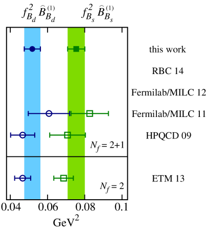
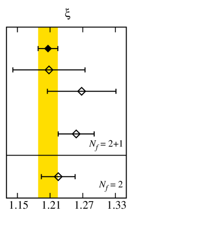
IX.2 Derived quantities
We now present quantities that are derived from the -mixing matrix element results in Table 13 that are especially useful for Standard-Model phenomenology.
IX.2.1 Ratios and other combinations of matrix elements
The SU(3)-breaking ratio , defined in Eq. (11), is needed for obtaining the ratio of CKM matrix elements from experimental measurements of the oscillation frequencies. The uncertainties on the individual matrix elements () in Table 13 are about 6–9 %, and are still substantially larger than the experimental errors on . Because the results for and are correlated, however, both the statistical and systematic uncertainties largely cancel in their ratio. We obtain
| (78) |
where again the first error is from the quadrature sum of the statistical and systematic uncertainties (the column labeled “Total” in Table 11) except for the charm-sea error, which is listed separately as a second error. Our result in Eq. (78) is consistent with the previous Fermilab/MILC result Bazavov et al. (2012a), , but about three times more precise due to the substantially increased data set and the inclusion of wrong-spin operators in the chiral-continuum extrapolation. Figure 15, right, compares our result with other unquenched lattice-QCD calculations.
We also present matrix-element combinations that enter the Standard-Model expression for the width difference . Following Ref. Lenz and Nierste (2007), we compute the -suppressed quantity , which is a linear combination of the matrix elements . The expression for is given in Eq. (13), where the NLO perturbative coefficients evaluated at the renormalization scale in the -BBGLN scheme are Lenz and Nierste (2007)
| (79) | |||||
| (80) |
We obtain
| (81) | |||||
| (82) |
where the errors are from the hadronic mixing matrix elements. The uncertainties from the parametric inputs and and the omission of charm sea quarks are negligible. Because the combination of operators in Eq. (13) is by construction -suppressed, our results for have larger relative errors than (which are of order 1 in the heavy-quark expansion), and may also be more sensitive to the systematic-uncertainty contributions considered previously. The stability of our results for under the fit modifications outlined in Sec. VIII.2.5, however, indicates that the quoted uncertainties adequately accommodate all sources of error. In Refs. Lenz and Nierste (2007); Artuso et al. (2015), the width difference is expressed in terms of bag parameters , rather than the matrix elements above. Our results for are given in Table 16 of Appendix A, which provides our complete set of bag-parameter results.
| Amhis et al. (2014) | |
IX.2.2 Bag parameters
The -mixing bag parameters are defined in Eqs. (6)–(8). We obtain their values from the matrix-element results in Table 13 by dividing by the appropriate factors of the leptonic decay constants and . We take the decay-constant averages from the recent PDG review Rosner et al. (2015):
| (83) |
which include lattice-QCD results from Refs. Bazavov et al. (2012b); McNeile et al. (2012); Carrasco et al. (2014b); Christ et al. (2015); Aoki et al. (2015). We use the three-flavor averages because we expect partial cancellations between the charm-sea effects in the decay constants and matrix elements to yield smaller overall errors on the bag parameters.
For the Standard-Model operator, we obtain the RGI bag parameters
| (84) | |||||
| (85) |
where the errors are from the matrix elements and the decay constants, respectively. Despite the reduction in errors on the matrix elements attained in this paper, the errors on our bag parameters are still similar in size to those of previous calculations because we use the PDG averages for the decay constants. Thus, we do not take advantage of the correlations and potential error cancellations that are possible in a combined analysis of -mixing matrix elements with the decay constants from the same lattice calculation. The SU(3)-breaking ratio of bag parameters for the Standard-Model operator is often used as an input for global CKM-unitarity-triangle fits Charles et al. (2005); Bona et al. (2006). We obtain
| (86) |
where the errors are from and , respectively. Here the bag-parameter ratio takes advantage of correlations between the - and -mixing matrix elements, making the error cancellation between the matrix elements and decay constants less important. Thus the decreased uncertainty on our result for in Eq. (78) translates into a commensurate error reduction on the bag-parameter ratio in Eq. (86). Our error for is 2–3 times smaller than the uncertainties quoted for previous three-flavor results Gámiz et al. (2009); Bazavov et al. (2012a); Aoki et al. (2015).
Table 15 in Appendix A gives results for the complete set of bag parameters (=1–5, ) in the -NDR scheme evaluated at the scale . It also provides the ratios for =2–5. The errors on the -parameters stem primarily from the matrix elements, and range from about 5–15%. To reduce the uncertainties, we are now performing a correlated, combined analysis of the mixing-matrix-elements in Table 13 with our own collaboration’s calculation of the decay constants using the same lattice ensembles and parameters Neil et al. (2015). The results will be reported in a future paper.
The values of the -parameters are all within about 20% of the vacuum-saturation-approximation expectation . A different definition of the -parameters for the mixed-chirality operators and is employed in Refs. Lenz and Nierste (2007, 2011); Artuso et al. (2015), which simplifies the expression for in the Standard Model, but results in bag parameters that are not equal to one in the VSA. Specifically, the term inside the brackets of Eq. (8) is set to one. To facilitate the use of our results in determinations of based on the expressions in Ref. Lenz and Nierste (2007), we provide the bag parameters and in the other convention, which are proportional to and , respectively, in Table 16 of Appendix A. The observed deviations from unity are greater than for and , being as much as 30% for .
The contributions to the errors on (=1–5) and (=0,1) from the decay constants are 100% correlated. Using this information, plus the correlations between the matrix elements given in Table 14, we obtain the correlations between the -parameters given in Table 17. This enables the calculation of observables that depend upon all possible combinations of bag parameters in Tables 15 and 16.
IX.3 Implications for Standard-Model phenomenology
We now illustrate the utility of the -mixing matrix elements given in Table 13 for Standard-Model phenomenology. First, we compute experimental observables associated with – mixing within the Standard Model. Next, assuming that the Standard Model is a complete description of Nature, we use the experimentally-measured oscillation frequencies to determine the associated CKM matrix elements , , and their ratio. Finally, we compute the total Standard-Model branching fractions for the rare decays . Table 12 provides the numerical inputs used for the calculations in this section.
IX.3.1 Oscillation frequencies
The physical observables associated with the neutral -meson system are the mass difference and the decay-width difference between the two mass eigenstates. Of these, the former have been measured at the sub-percent level Amhis et al. (2014):
| (87) |
while the width differences have been measured with larger uncertainties Amhis et al. (2014),
| (88) |
The average for from the Heavy Flavor Averaging Group (HFAG) in Eq. (87) is based on over 30 measurements and is dominated by results from the Belle, BaBar, and LHCb experiments Abe et al. (2005); Aubert et al. (2006); Aaij et al. (2013b), while the average for is obtained from measurements from the CDF and LHCb experiments Abulencia et al. (2006); Aaij et al. (2012, 2013c, 2013d, 2015a). The average is obtained from measurements by the Delphi, BaBar, Belle, D0, and LHCb experiments Abdallah et al. (2003); Aubert et al. (2004a, b); Higuchi et al. (2012); Abazov et al. (2014); Aaij et al. (2014a) and the average is based on measurements by the CDF, ATLAS, CMS, and LHCb experiments Aaltonen et al. (2012); Abazov et al. (2012); Aad et al. (2014); Khachatryan et al. (2015a); Aaij et al. (2015a).
Equation (10) gives the expression for the mass difference in the Standard Model. Using the hadronic matrix elements from Table 13 and from Eq. (78) and other numerical inputs from Table 12, we obtain
| (89) | |||||
| (90) | |||||
| (91) |
where the errors shown are from the theoretical errors on the mixing matrix elements, the CKM matrix elements, the remaining parametric inputs to Eq. (10), and the omission of charm sea quarks, respectively. Note that, for the CKM parameters, we use the determination from the CKMfitter Group’s analysis including only tree-level observables because it does not utilize the constraints from -meson mixing.
The Standard-Model values for above have significantly larger uncertainties than the experimental averages quoted in Eqs. (87). The dominant error in the theoretical calculation of stems from the hadronic mixing matrix elements. For and , the hadronic matrix-element and CKM uncertainties are commensurate. Our results for , , and differ from experiment by 1.8, 1.1, and 2.0, respectively.
IX.3.2 CKM matrix elements and
In the Standard Model, the neutral -meson oscillation frequencies [Eq. (10)] are proportional to the combination of CKM matrix elements . Therefore experimental measurements of and enable determinations of , , and their ratio, within the Standard-Model CKM framework. At present, the errors on these determinations Olive et al. (2014) are limited by the theoretical uncertainties on the hadronic -mixing matrix elements Gámiz et al. (2009); Bazavov et al. (2012a). Here we improve upon them using our new, more precise matrix-element calculations.
We take the results for () from Table 13 and for from Eq. (78), and use the experimental averages for in Eq. (87) Amhis et al. (2014). The other numerical inputs that enter the expressions for are given in Table 12. To infer values for the individual matrix elements and , we take from CKM unitarity Charles et al. (2005), where the error is of and hence negligible. We obtain
| (92) | |||||
| (93) | |||||
| (94) |
where the errors are from the lattice mixing matrix elements, the measured , the remaining parametric inputs to Eq. (10), and the omission of charm sea quarks, respectively. The uncertainty on is 2–3 times smaller than those on and individually because the hadronic uncertainties are suppressed in the ratio. The theoretical uncertainties from the -mixing matrix elements are still, however, the dominant sources of error in all three results in Eqs. (92)–(94).
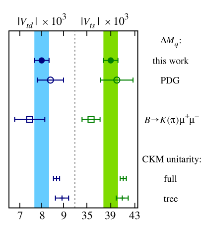
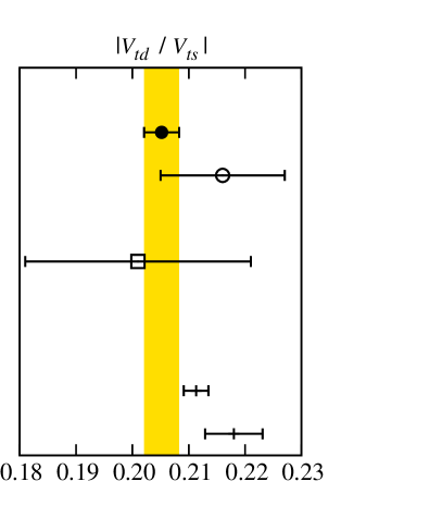
Our results are consistent with the values from -meson mixing in the PDG review Olive et al. (2014), which are obtained using approximately the same experimental inputs, and lattice-QCD calculations of the and from Refs. Gámiz et al. (2009) and Bazavov et al. (2012a), respectively. Our errors on , are about two times smaller, however, and on they are more than three times smaller, due to the reduced theoretical errors on the hadronic matrix elements.
The CKM matrix elements and can be obtained independently from rare semileptonic -meson decays because the Standard-Model rates for are proportional to the same combination . Until recently, these determinations were not competitive with those from -meson mixing due to both large experimental and theoretical uncertainties. In the past year, however, the LHCb collaboration published new measurements of and Aaij et al. (2014b, 2015b), and we calculated the full set of and form factors in three-flavor lattice QCD Bailey et al. (2015a, b). Using these results, Ref. Du et al. (2016) obtains
| (95) | |||||
| (96) | |||||
| (97) |
where the errors include all sources of uncertainty. These determinations of and agree with our -mixing results in Eqs. (92) and (94), while above differs from Eq. (93) by about 1.6.
It is instructive to compare these results for , , and from mixing and rare semileptonic decays with expectations from CKM unitarity. These processes, being mediated by flavor-changing-neutral currents (FCNCs), may receive observable contributions from new physics. Figure 16 shows two sets of CKM elements inferred from unitarity, labeled “full” and “tree,” which are obtained, respectively, from CKMfitter’s full global unitarity-triangle fit using all inputs Charles et al. (2005) and from a fit including only observables that are mediated at the tree level of the weak interactions Descotes-Genon . With the improvements in this paper for the -mixing matrix elements, and in Refs. Aaij et al. (2014b, 2015b); Bailey et al. (2015a, b); Du et al. (2016) for rare semileptonic decay form factors, a discrepancy between FCNC and tree-level processes may be emerging. Quantitatively, the -mixing results for and differ from the tree-fit values by and , and their ratio by . 333These CKM discrepancies are not distinct from those observed for in Eqs. (89)–(91), but the CKM perspective is convenient for contrasting the role of different observables. Similarly, the FCNC semileptonic decays yield values of and that lie, respectively, and below the CKM tree-fit results. (The comparison of from FCNC semileptonic decays is not yet useful because of the large experimental uncertainties.) The overall impression does not change qualitatively when comparing with the results of the full CKM unitarity-triangle fit: , , and from mixing differ by 1.8, 1.5, and 1.5, respectively; and from FCNC semileptonic decays differ by and , respectively. It would be interesting to see whether new flavor-changing neutral currents could explain this pattern, but such a study lies beyond the scope of this work.
IX.3.3 Branching ratios for
The rare decays () also proceed via flavor-changing neutral currents, and are therefore similarly sensitive to physics beyond the Standard Model. Revealing the presence of such effects, however, requires both precise experimental measurements and reliable theoretical predictions with commensurate uncertainties. Here we calculate the Standard-Model rates for using our calculations of the -mixing matrix elements in Table 13.
The expression for the Standard-Model rate is given in, e.g., Eq. (3) of Ref. Bobeth et al. (2014b), and depends upon the leptonic decay constant and the combination of CKM matrix elements . The Standard-Model predictions receive substantial error contributions from both the CKM matrix elements and the decay constants, as shown in Eqs. (106) and (107) below. Buras pointed out Buras (2003), however, that the same CKM matrix elements also enter the Standard-Model expression for the neutral -mixing oscillation frequency . Thus, the ratio is independent of both and , although it still depends upon the hadronic bag parameter . Assuming that new physics does not alter the frequency of -meson oscillations, this cancellation potentially enables more precise Standard-Model predictions for and , since the relevant CKM combinations have large uncertainties, whereas the oscillation frequencies have been measured to better than a percent.
In the Standard Model, the ratio of the decay rate over the -meson mass difference is given by Buras (2003); Bobeth et al. (2014b)
| (98) |
where the Wilson coefficient includes NLO electroweak and NNLO QCD corrections Hermann et al. (2013); Bobeth et al. (2014c) and the remaining quantities are the same as in the expression for [Eq. (10)]. For the decay mode, the nonzero gives rise to a difference between the experimentally measured, time-integrated decay rate and the theoretical, CP-averaged rate De Bruyn et al. (2012a, b); Buras et al. (2013). Following Ref. Bobeth et al. (2014b), we use the lifetime of the heavy -meson eigenstate to compute the time-averaged branching fraction as , which holds when only the heavy eigenstate can decay to , as in the Standard Model. (In the case of the system, , because .) For the double ratio of -to- processes, the expression simplifies to
| (99) |
Using the bag-parameter results from Eqs. (84)–(86), and the numerical inputs from Table 12, we obtain
| (100) | |||||
| (101) |
and
| (102) |
where the errors shown are from the theoretical errors on the bag parameters, and all other uncertainties added in quadrature, respectively. Multiplying the ratios in Eqs. (100)–(102) by the oscillation frequencies from Eq. (87) Amhis et al. (2014), we obtain the following Standard-Model total rates:
| (103) | |||||
| (104) | |||||
| (105) |
where the errors shown are from the theoretical errors on the bag parameters, the measured , and the quadrature sum of all other sources of uncertainty, respectively. The bag parameters are the dominant source of uncertainty. Because our bag-parameter errors are comparable to those of previous calculations, our decay-rate results in Eqs. (103) and (104) are similar in precision to those presented in Ref. Bobeth et al. (2014b).
We can also compare our predictions with the Standard-Model decay rates calculated via Eqs. (6) and (7) of Ref. Bobeth et al. (2014b):
| (106) | |||||
| (107) | |||||
| (108) |
where the errors are from the decay constants, CKM matrix elements, and the quadrature sum of all other contributions, respectively. For the calculations of Eqs. (106)–(108), we use the PDG’s preferred decay-constant averages
| (109) |
which include both three- and four-flavor lattice-QCD results Bazavov et al. (2012b); McNeile et al. (2012); Dowdall et al. (2013); Carrasco et al. (2014b); Christ et al. (2015); Aoki et al. (2015), because they are the most precise available. In this case, the contributions to the error on the total decay rates from the three sources of uncertainty are similar in size. The uncertainties in Eqs. (103)–(105) are slightly larger than those in Eqs. (106)–(108). The central values differ only slightly by 1.3, 1.2, and 1.2, respectively.
Recently the LHCb and CMS experiments reported the first observation of decay, as well as 3 evidence for the process Khachatryan et al. (2015b), obtaining
| (110) | |||||
| (111) | |||||
| (112) |
The measured branching fraction for is compatible with our Standard-Model value in Eq. (104), within present uncertainties, but there is still ample room for new-physics contributions of a size that may be observable with improved experimental measurements after the LHC luminosity upgrade. The measured branching fraction for is 2.0 above the Standard-Model expectation in Eq. (103) after averaging the asymmetric experimental errors, while the measured ratio lies 1.6 above the result in Eq. (105). The measurement errors must be reduced, however, before one can draw meaningful conclusions.
X Conclusions and outlook
We have presented the first three-flavor lattice-QCD results for the -meson () mixing matrix elements of the full set of dimension-six four-fermion operators in the electroweak effective Hamiltonian. The first matrix element is needed to calculate the mass differences in the Standard Model, while the remaining four matrix elements (=2–5) are sufficient to parameterize the hadronic contributions to in any Standard-Model extension. These matrix elements are also sufficient to obtain the leading-order contributions to the Standard-Model width differences , as well as some of the corrections of order . For the Standard-Model matrix element , we obtain the renormalization-group-invariant combinations
| (113) | ||||
| (114) |
where the first error includes statistical and all systematic uncertainties except for the charm-sea error, which is shown separately. Our results for the complete set of matrix elements (1–5) are given in Table 13. To enable the use of our lattice -meson mixing matrix elements for additional phenomenological studies, we provide the correlations between them in Table 14.
Although there have been previous three-flavor lattice-QCD calculations of the matrix elements of the Standard-Model operator , ours are the first with all sources of systematic uncertainty controlled. In particular, compared with Refs. Gámiz et al. (2009); Bouchard et al. (2011); Bazavov et al. (2012a), we include the contributions from wrong-spin operators in the chiral continuum-extrapolation. Our analysis also includes ensembles with finer lattice spacings and lighter pions than in previous works. We obtain the SU(3)-breaking ratio
| (115) |
to 1.6% precision, which is the most precise lattice-QCD determination of this quantity to-date. The reduction in errors by about a factor of three compared with our earlier work Bazavov et al. (2012a) is due in large part to correctly handling the wrong-spin operators in the chiral-continuum extrapolation. The total uncertainty is now definitively smaller than that quoted in many early estimates—see, for example, Refs. Ciuchini et al. (2001); Höcker et al. (2001)—in which the uncertainty from the chiral extrapolation was underestimated Kronfeld and Ryan (2002).
To illustrate the phenomenological utility of our -mixing matrix elements, we have used them to calculate the mass differences and the total branching fractions for the rare-decay processes in the Standard Model, where we highlight the ratios in which the CKM factors and decay constants cancel. The Standard-Model expectations for , , and their ratio are all greater than the experimental averages, where the differences are 1.8, 1.1, and 2.0, respectively. The Standard-Model rate for lies 2.0 below experiment, although one should bear in mind that the experimental observation of decay has yet to reach 5 significance.
We also obtain the CKM matrix elements , , and their ratio assuming that there are no significant new-physics contributions to -meson oscillations. The results
| (116) | ||||
| (117) | ||||
| (118) |
are the single-most precise determinations of these quantities, and differ with expectations from CKM unitarity Charles et al. (2005); Bona et al. (2006). (As above, the semiquantitative charm-sea error is listed separately from the other uncertainties.) The CKM-element results from -meson mixing lie below the determinations from CKMfitter’s full global unitarity-triangle fit using all inputs by 1.5–1.8, and below the determinations using only tree-level inputs by 1.2–2.1 Charles et al. (2005). Because our new -mixing matrix elements imply lower values for , , and their ratio, they enhance the observed tension between tree-level and loop-induced processes Charles et al. (2005).
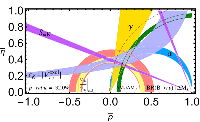
Figure 17 shows the current status of the CKM unitarity triangle using our new result for plus recent determinations of and from our calculations of the and form factors Bailey et al. (2015c, a).444We obtain this value of from a fit similar to the one in Ref. DeTar (2015) including the recent measurements from Belle Glattauer et al. (2015), earlier measurements from BaBar Aubert et al. (2009), and our lattice-QCD form factors from Ref. Bailey et al. (2015a). At present, the experimental measurements are compatible with the Standard Model at . The overall precision still leaves ample room for BSM flavor-changing neutral currents that may be observable with anticipated theoretical improvements such as those discussed below, in conjunction with more precise experimental measurements expected from the LHC upgrade Aaij et al. (2013a); The CMS Collaboration (2015) and Belle II Aushev et al. (2010).
Despite the improvement in the -mixing elements obtained in this paper, the theoretical hadronic errors are still the limiting source of uncertainty in all calculations of observables in Sec. IX. In a forthcoming paper, we will report bag-parameter results from a combined analysis of the mixing-matrix-elements presented here with our collaboration’s companion decay-constant calculation using the same lattice ensembles and parameters Neil et al. (2015). We anticipate that the inclusion of statistical and systematic correlations between the matrix elements and decay constants will reduce the bag-parameter errors, thereby enabling better predictions of the decay rates and other observables.
Additional work is still needed, however, to reduce the QCD uncertainties to the level of experimental measurements. The dominant errors in our current matrix-element results stem from statistics and heavy-quark discretization errors. The contribution from the chiral extrapolation is also significant for the matrix elements and . We plan to reduce these uncertainties by using the newly generated gauge-field ensembles by the MILC Collaboration Bazavov et al. (2010a, 2013) with four flavors of highly-improved staggered quarks (HISQ) Follana et al. (2007). Ensembles with physical-mass pions at four lattice spacings are already available, the use of which will render the chiral extrapolation unnecessary and eliminate the associated systematic uncertainty. In addition, the inclusion of charm quarks in the sea will eliminate the least-well quantified source of error in our current calculation. The inclusion of ensembles at an even finer lattice spacing will be particularly important for reducing heavy-quark discretization effects. Such a fine lattice spacing will also be useful in calculations that employ the HISQ action for the quark McNeile et al. (2012). Finally, because the matrix elements are dimensionful, they also receive error contributions from the lattice-spacing uncertainty, which will become relatively more important as the other errors discussed above are reduced. Recently several new scale-setting quantities have been introduced Lüscher (2010); Borsanyi et al. (2012); Bazavov et al. (2013, 2015) that can be obtained more directly and precisely than , one of which has already been employed in our calculation of charmed and light pseudoscalar-meson decay constants on the HISQ ensembles Bazavov et al. (2014).
Once the matrix-element errors reach the few-percent level, it will be important to provide the -mixing matrix elements at the correct physical -quark mass. This can be done straightforwardly, as we have shown in this work, by including partially-quenched data in the analysis, and then evaluating the chiral fit function with the valence-quark mass equal to and the sea-quark masses equal to the average up-down quark mass. For calculations where only full-QCD data is available, the corrections listed in Table 10 can be used to adjust the isospin-averaged -mixing matrix elements for valence isospin breaking.
Neutral -meson mixing provides a powerful test of the Standard Model and stringent constraints on new, high-scale physics Isidori et al. (2010); Lenz et al. (2011); Carrasco et al. (2014a). Our work reveals several deviations between the Standard Model and experiment in -meson oscillations and rare leptonic decays. Similar-sized tensions have been observed in rare semileptonic decays Aaij et al. (2013e, 2014c); Altmannshofer and Straub (2015); Langenbruch (2015); Du et al. (2016), which also proceed via and flavor-changing neutral currents. The full basis of mixing matrix elements, including their correlations, provided here will allow these interesting tensions to be better explored, leading to sharper tests of the Standard Model and tighter constraints on allowed new physics.
Acknowledgements.
We thank Sébastien Descotes-Genon for helpful discussions and supplementary information on CKMfitter’s results, Enrico Lunghi for providing the global unitarity-triangle fit plot and assisting in calculations of observables, and Andrzej Buras, Martin Jung, and Alexander Lenz for helpful discussions and valuable feedback on the manuscript. Computations for this work were carried out with resources provided by the USQCD Collaboration, the National Energy Research Scientific Computing Center and the Argonne Leadership Computing Facility, which are funded by the Office of Science of the U.S. Department of Energy; and with resources provided by the National Institute for Computational Science and the Texas Advanced Computing Center, which are funded through the National Science Foundation’s Teragrid/XSEDE Program. This work was supported in part by the U.S. Department of Energy under grants No. DE-FG02-91ER40628 (C.B.) No. DE-FC02-06ER41446 (C.D.) No. DE-SC0010120 (S.G.), No. DE-SC0010005 (E.T.N.), No. DE-FG02-91ER40661 (S.G., R.Z.), No. DE-FG02-13ER42001 (C.C.C., D.D., A.X.K.), No. DE-FG02-13ER41976 (D.T.); by the U.S. National Science Foundation under grants PHY10-67881 and PHY10-034278 (C.D.), PHY14-17805 (D.D., J.L.), and PHY13-16748 (R.S.); by the Fermilab Fellowship in Theoretical Physics (C.M.B., C.C.C.); by the URA Visiting Scholars’ program (C.M.B., C.C.C., D.D., A.X.K.); by the MICINN (Spain) under grant FPA2010-16696 and Ramón y Cajal program (E.G.); by the Junta de Andalucía (Spain) under Grants No. FQM-101 and No. FQM-6552 (E.G.); by the European Commission (EC) under Grant No. PCIG10-GA-2011-303781 (E.G.); by the German Excellence Initiative and the European Union Seventh Framework Program under grant agreement No. 291763 as well as the European Union’s Marie Curie COFUND program (A.S.K.). Fermilab is operated by Fermi Research Alliance, LLC, under Contract No. DE-AC02-07CH11359 with the United States Department of Energy. Brookhaven National Laboratory is supported by the DoE under contract no. DE-SC0012704.Appendix A Numerical results for -mixing matrix elements and bag parameters
Tables 13–17 in this Appendix present our results for the complete set of -mixing matrix elements and bag parameters with total statistical plus systematic uncertainties, as well as the correlations between them. The bag parameters are defined in Eqs. (6)–(8) to be one in the vacuum saturation approximation. This information is sufficient to use our results in calculations of -mixing observables both within and beyond the Standard Model.
Because the estimated uncertainty due to the omission of charm sea quarks is less quantitative than the other uncertainties, we do not provide correlations for this error. Rather we suggest that an error of 2% be taken on all sums or differences of matrix elements (; =1–5), and that an error of 0.5% be taken on all ratios of (sums or differences of) -to- matrix elements. As discussed earlier, we consider the charm-sea error in the bag parameters and same-flavor matrix-element ratios to be negligible.
| – | – | |||
| BMU | BBGLN | BMU | BBGLN | |
| 0.0342(29)(7) | 0.0498(30)(10) | |||
| 0.0285(26)(6) | 0.0303(27)(6) | 0.0421(27)(8) | 0.0449(29)(9) | |
| 0.0402(77)(8) | 0.0399(77)(8) | 0.0576(77)(12) | 0.0571(77)(11) | |
| 0.0390(28)(8) | 0.0534(30)(11) | |||
| 0.0361(35)(7) | 0.0493(36)(10) | |||
| 1 | 0.378 | 0.070 | 0.336 | 0.287 | 0.968 | 0.395 | 0.089 | 0.346 | 0.305 | |
| 1 | 0.212 | 0.348 | 0.255 | 0.394 | 0.961 | 0.230 | 0.365 | 0.277 | ||
| 1 | 0.134 | 0.065 | 0.079 | 0.207 | 0.980 | 0.137 | 0.071 | |||
| 1 | 0.404 | 0.371 | 0.391 | 0.162 | 0.955 | 0.426 | ||||
| 1 | 0.309 | 0.281 | 0.084 | 0.404 | 0.962 | |||||
| 1 | 0.455 | 0.117 | 0.419 | 0.359 | ||||||
| 1 | 0.253 | 0.453 | 0.339 | |||||||
| 1 | 0.186 | 0.107 | ||||||||
| 1 | 0.471 | |||||||||
| 1 |
| – | – | |||
| BMU | BBGLN | BMU | BBGLN | |
| 0.913(76)(40) | 0.952(58)(32) | |||
| 0.761(68)(33) | 0.808(72)(35) | 0.806(52)(27) | 0.859(55)(29) | |
| 1.07(21)(5) | 1.07(21)(5) | 1.10(15)(4) | 1.09(15)(4) | |
| 1.040(75)(45) | 1.022(57)(34) | |||
| 0.964(93)(42) | 0.943(68)(31) | |||
| 0.838(81) | 0.885(73) | 0.849(56) | 0.902(59) | |
| 1.18(24) | 1.17(24) | 1.16(16) | 1.15(16) | |
| 1.14(10) | 1.073(68) | |||
| 1.06(11) | 0.990(75) | |||
| – | – | |
|---|---|---|
| 0.32(73)(1) | 0.52(52)(2) | |
| 1.57(11)(7) | 1.536(84)(51) | |
| 1.19(11)(5) | 1.165(84)(39) | |
| 0.35(80) | 0.54(55) | |
| 1.72(15) | 1.61(10) | |
| 1.31(14) | 1.223(93) |
| 1 | 0.504 | 0.162 | 0.494 | 0.422 | -0.231 | 0.500 | 0.423 | 0.754 | 0.311 | 0.077 | 0.264 | 0.246 | -0.235 | 0.269 | 0.247 | |
| 1 | 0.282 | 0.494 | 0.389 | 0.528 | 0.477 | 0.380 | 0.311 | 0.766 | 0.201 | 0.283 | 0.226 | 0.509 | 0.259 | 0.214 | ||
| 1 | 0.225 | 0.148 | -0.456 | 0.216 | 0.143 | 0.068 | 0.179 | 0.929 | 0.115 | 0.063 | -0.454 | 0.103 | 0.057 | |||
| 1 | 0.528 | 0.036 | 0.988 | 0.518 | 0.279 | 0.297 | 0.134 | 0.705 | 0.332 | 0.030 | 0.688 | 0.319 | ||||
| 1 | 0.032 | 0.523 | 0.998 | 0.247 | 0.228 | 0.074 | 0.318 | 0.797 | 0.026 | 0.310 | 0.794 | |||||
| 1 | 0.036 | 0.031 | -0.212 | 0.469 | -0.443 | 0.031 | 0.027 | 0.982 | 0.031 | 0.027 | ||||||
| 1 | 0.524 | 0.283 | 0.270 | 0.120 | 0.683 | 0.322 | 0.030 | 0.696 | 0.323 | |||||||
| 1 | 0.248 | 0.214 | 0.067 | 0.305 | 0.793 | 0.026 | 0.311 | 0.796 | ||||||||
| 1 | 0.575 | 0.215 | 0.560 | 0.486 | -0.196 | 0.571 | 0.488 | |||||||||
| 1 | 0.329 | 0.581 | 0.466 | 0.498 | 0.553 | 0.450 | ||||||||||
| 1 | 0.278 | 0.195 | -0.437 | 0.263 | 0.186 | |||||||||||
| 1 | 0.581 | 0.057 | 0.981 | 0.565 | ||||||||||||
| 1 | 0.048 | 0.574 | 0.996 | |||||||||||||
| 1 | 0.058 | 0.048 | ||||||||||||||
| 1 | 0.577 | |||||||||||||||
| 1 |
Appendix B Evaluating quality of fits
In this Appendix, we discuss the measures of goodness of fit used to guide and scrutinize the analysis. All fits presented in this work take the correlations between the data into account. As discussed below, it is (conceptually) necessary to constrain the fit parameters, and we do so with Gaussian priors.
We evaluate the quality of our fit results with two test statistics denoted and , both of which are defined via the (complementary) cumulative distribution with degrees of freedom Olive et al. (2014):
| (119) |
which gives the probability that a random -component vector satisfies . The statistics and differ in the choices made for and in this formula.
With a finite set of parameters in a theoretical model, it is customary to form the function
| (120) |
where is the parameter vector, denotes the fit model, the data, and is the covariance matrix between the data. One then finds the parameter vector that minimizes . A good model, fit to many similar data sets, should yield for a uniform distribution over , where and are the numbers of data points and fitted parameters, respectively.
In the cases at hand—correlator fits and the chiral-continuum extrapolation—there are, in principle, infinitely many parameters. Because only the first few terms in the tower of states in Eqs. (25) and (28) or in the PT expansion in Sec. VII can be determined by the data, one must in practice constrain all but a few parameters. Note that truncating the tower of states or the order in PT is the same as constraining all omitted terms to vanish. Fits are more stable over a wider range of data when one includes several higher-order parameters that are constrained moderately with priors instead of sharply truncating the series.
We thus introduce an “augmented” function Lepage et al. (2002):
| (121) |
imposing prior distributions for parameters with prior central values and covariance matrix . In practice, we take the priors to be uncorrelated, i.e., is diagonal. Further, we impose a prior for every parameter actively fit, including those well-constrained by the data. Our best-fit parameter vector is the one that minimizes .
Each prior is an additional piece of information, so we examine
| (122) |
to rank the quality of the fits. When carrying out many similar fits, the resulting values need not follow a uniform distribution, because need not follow the distribution for degrees of freedom. A uniform distribution for arises only when the priors have been chosen such that the extra terms in Eq. (121) make a contribution , i.e., when the prior widths are narrow.
Our priors are not chosen to yield such an outcome. Instead, the priors for the essential fit parameters are effectively unconstraining, and the others are chosen to promote fit stability. Nevertheless, we find to be useful when ranking fits with different . To test the influence of the priors on the best fit, we introduce a value via
| (123) |
omitting from the terms corresponding to the priors, but still using the best-fit parameter vector that minimizes . If the priors do not influence the fits in an undesirable way, then should be close enough to that the value in Eq. (123) is uniformly distributed between 0 and 1. Figure 9 shows this to be the case for the correlator fits.
Appendix C Chiral logarithms
For reasons discussed in Sec. VII.1.1, we use a notation for the loop-diagram functions that is slightly different than in the original paper Bernard (2013). Here we provide a dictionary to translate between this work and Ref. Bernard (2013).
In this paper, the light valence quark ( or ) is labeled with but in Ref. Bernard (2013) with . Here, the index denotes the five operators, but in Ref. Bernard (2013) is used. Thus, when a label on the functions corresponds to these properties, the notation will differ in a trivial way.
We follow the notation of Ref. Bernard (2013) for correct-spin contributions. The self-energy function is given explicitly in Eq. (62) of Ref. Bernard (2013). The correct-spin tadpole functions depend on whether or ; and are given in Eqs. (82) and (83), respectively, of Ref. Bernard (2013). The sunset function is the same for all (or ); is given in Eq. (89) of Ref. Bernard (2013).
For the wrong-spin contributions, we find it more transparent to separate the LECs from the loop-diagram functions. The relation between our notation (left-hand side) and that of Ref. Bernard (2013) (right-hand side) is as follows:
| (124a) | ||||
| (124b) | ||||
| (124c) | ||||
| (124d) | ||||
| (124e) | ||||
and
| (125a) | ||||
| (125b) | ||||
| (125c) | ||||
| (125d) | ||||
| (125e) | ||||
Equations (124) can be obtained from Eqs. (84)–(88) of Ref. Bernard (2013), and Eqs. (125) from Eqs. (90)–(94) of that paper.
References
- Hewett et al. (2012) J. L. Hewett, H. Weerts, et al., Fundamental Physics at the Intensity Frontier (U.S. Department of Energy, 2012) arXiv:1205.2671 [hep-ex] .
- Isidori et al. (2010) G. Isidori, Y. Nir, and G. Perez, Annu. Rev. Nucl. Part. Sci. 60, 355 (2010), arXiv:1002.0900 [hep-ph] .
- Buras and Girrbach (2014) A. J. Buras and J. Girrbach, Rept. Prog. Phys. 77, 086201 (2014), arXiv:1306.3775 [hep-ph] .
- Buras et al. (2014a) A. J. Buras, D. Buttazzo, J. Girrbach-Noe, and R. Knegjens, JHEP 11, 121 (2014a), arXiv:1408.0728 [hep-ph] .
- de Gouvea et al. (2013) A. de Gouvea et al. (Neutrino Working Group), (2013), arXiv:1310.4340 [hep-ex] .
- Dawson et al. (2013) S. Dawson et al. (Higgs Boson Working Group), (2013), arXiv:1310.8361 [hep-ex] .
- Butler et al. (2013) J. N. Butler et al. (Quark Flavor Physics Working Group), (2013), arXiv:1311.1076 [hep-ex] .
- Albrecht et al. (2013) J. Albrecht et al. (Charged Leptons Working Group), (2013), arXiv:1311.5278 [hep-ex] .
- Amhis et al. (2014) Y. Amhis et al. (Heavy Flavor Averaging Group), (2014), online update at http://www.slac.stanford.edu/xorg/hfag/, arXiv:1412.7515 [hep-ex] .
- Aaij et al. (2013a) R. Aaij et al. (LHCb), Eur. Phys. J. C73, 2373 (2013a), arXiv:1208.3355 [hep-ex] .
- Aushev et al. (2010) T. Aushev et al., (2010), arXiv:1002.5012 [hep-ex] .
- Dalgic et al. (2007) E. Dalgic, A. Gray, E. Gámiz, C. T. H. Davies, G. P. Lepage, J. Shigemitsu, H. Trottier, and M. Wingate (HPQCD), Phys. Rev. D76, 011501 (2007), arXiv:hep-lat/0610104 [hep-lat] .
- Gámiz et al. (2009) E. Gámiz, C. T. H. Davies, G. P. Lepage, J. Shigemitsu, and M. Wingate (HPQCD), Phys. Rev. D80, 014503 (2009), arXiv:0902.1815 [hep-lat] .
- Albertus et al. (2010) C. Albertus et al. (RBC and UKQCD), Phys. Rev. D82, 014505 (2010), arXiv:1001.2023 [hep-lat] .
- Bazavov et al. (2012a) A. Bazavov et al. (Fermilab Lattice and MILC), Phys. Rev. D86, 034503 (2012a), arXiv:1205.7013 [hep-lat] .
- Carrasco et al. (2014a) N. Carrasco et al. (ETM), JHEP 03, 016 (2014a), arXiv:1308.1851 [hep-lat] .
- Aoki et al. (2015) Y. Aoki, T. Ishikawa, T. Izubuchi, C. Lehner, and A. Soni, Phys. Rev. D91, 114505 (2015), arXiv:1406.6192 [hep-lat] .
- Eichten and Hill (1990) E. Eichten and B. R. Hill, Phys. Lett. B240, 193 (1990).
- Hasenfratz and Knechtli (2001) A. Hasenfratz and F. Knechtli, Phys. Rev. D64, 034504 (2001), arXiv:hep-lat/0103029 [hep-lat] .
- Della Morte et al. (2005) M. Della Morte, A. Shindler, and R. Sommer (ALPHA), JHEP 08, 051 (2005), arXiv:hep-lat/0506008 [hep-lat] .
- Dowdall et al. (2014) R. J. Dowdall, C. T. H. Davies, R. R. Horgan, G. P. Lepage, C. J. Monahan, and J. Shigemitsu (HPQCD), PoS LATTICE2014, 373 (2014), arXiv:1411.6989 [hep-lat] .
- Lepage et al. (1992) G. P. Lepage, L. Magnea, C. Nakhleh, U. Magnea, and K. Hornbostel, Phys. Rev. D46, 4052 (1992), arXiv:hep-lat/9205007 [hep-lat] .
- Gámiz et al. (2008) E. Gámiz, J. Shigemitsu, and H. Trottier, Phys. Rev. D77, 114505 (2008), arXiv:0804.1557 [hep-lat] .
- Hammant et al. (2013) T. C. Hammant, A. G. Hart, G. M. von Hippel, R. R. Horgan, and C. J. Monahan, Phys. Rev. D88, 014505 (2013), arXiv:1303.3234 [hep-lat] .
- Bazavov et al. (2010a) A. Bazavov et al. (MILC), Phys. Rev. D82, 074501 (2010a), arXiv:1004.0342 [hep-lat] .
- Bazavov et al. (2013) A. Bazavov et al. (MILC), Phys. Rev. D87, 054505 (2013), arXiv:1212.4768 [hep-lat] .
- Bernard et al. (2001) C. W. Bernard, T. Burch, K. Orginos, D. Toussaint, T. A. DeGrand, S. Datta, C. DeTar, S. Gottlieb, U. M. Heller, K. Orginos, R. Sugar, and D. Toussaint, Phys. Rev. D64, 054506 (2001), arXiv:hep-lat/0104002 [hep-lat] .
- Aubin et al. (2004a) C. Aubin, C. Bernard, C. E. DeTar, J. Osborn, S. Gottlieb, E. B. Gregory, D. Toussaint, U. M. Heller, J. E. Hetrick, and R. Sugar, Phys. Rev. D70, 094505 (2004a), arXiv:hep-lat/0402030 [hep-lat] .
- Bazavov et al. (2010b) A. Bazavov et al., Rev. Mod. Phys. 82, 1349 (2010b), arXiv:0903.3598 [hep-lat] .
- Bouchard et al. (2011) C. M. Bouchard, E. D. Freeland, C. Bernard, A. X. El-Khadra, E. Gámiz, A. S. Kronfeld, J. Laiho, and R. S. Van de Water, PoS LATTICE2011, 274 (2011), arXiv:1112.5642 [hep-lat] .
- Hansmann-Menzemer and Nierste (2015) S. Hansmann-Menzemer and U. Nierste, in The Large Hadron Collider: Harvest of Run 1, edited by T. Schörner-Sadenius (Springer, Berlin, 2015) pp. 301–353.
- Buras (2015) A. Buras, PoS FWNP, 003 (2015), arXiv:1505.00618 [hep-ph] .
- Nierste (2013) U. Nierste, J. Phys. Conf. Ser. 447, 012017 (2013), arXiv:1304.3831 [hep-ph] .
- Lenz (2014) A. Lenz, in 8th International Workshop on the CKM Unitarity Triangle (CKM2014) Vienna, Austria, September 8-12, 2014 (2014) arXiv:1409.6963 [hep-ph] .
- Bobeth (2014) C. Bobeth, J. Phys. Conf. Ser. 556, 012039 (2014).
- Borissov et al. (2013) G. Borissov, R. Fleischer, and M.-H. Schune, Ann. Rev. Nucl. Part. Sci. 63, 205 (2013), arXiv:1303.5575 [hep-ph] .
- Blanke et al. (2015) M. Blanke, A. J. Buras, and S. Recksiegel, (2015), arXiv:1507.06316 [hep-ph] .
- Buras et al. (2014b) A. J. Buras, F. De Fazio, and J. Girrbach-Noe, JHEP 08, 039 (2014b), arXiv:1405.3850 [hep-ph] .
- Buras et al. (2014c) A. J. Buras, F. De Fazio, and J. Girrbach, JHEP 02, 112 (2014c), arXiv:1311.6729 [hep-ph] .
- Buras and Girrbach (2013) A. J. Buras and J. Girrbach, Eur. Phys. J. C73, 2560 (2013), arXiv:1304.6835 [hep-ph] .
- Lenz et al. (2011) A. Lenz, U. Nierste, J. Charles, S. Descotes-Genon, A. Jantsch, C. Kaufhold, H. Lacker, S. Monteil, V. Niess, and S. T’Jampens (CKMfitter), Phys. Rev. D83, 036004 (2011), arXiv:1008.1593 [hep-ph] .
- Lenz et al. (2012) A. Lenz, U. Nierste, J. Charles, S. Descotes-Genon, H. Lacker, S. Monteil, V. Niess, and S. T’Jampens, Phys. Rev. D86, 033008 (2012), arXiv:1203.0238 [hep-ph] .
- Brod et al. (2015) J. Brod, A. Lenz, G. Tetlalmatzi-Xolocotzi, and M. Wiebusch, Phys. Rev. D92, 033002 (2015), arXiv:1412.1446 [hep-ph] .
- Bobeth et al. (2014a) C. Bobeth, U. Haisch, A. Lenz, B. Pecjak, and G. Tetlalmatzi-Xolocotzi, JHEP 06, 040 (2014a), arXiv:1404.2531 [hep-ph] .
- Shimizu et al. (2013) Y. Shimizu, M. Tanimoto, and K. Yamamoto, Phys. Lett. B726, 747 (2013), arXiv:1307.0374 [hep-ph] .
- Kim and Zurek (2014) I.-W. Kim and K. M. Zurek, Phys. Rev. D89, 035008 (2014), arXiv:1310.2617 [hep-ph] .
- Nelson and Scholtz (2015) A. E. Nelson and J. Scholtz, Phys. Rev. D91, 014009 (2015), arXiv:1311.0040 [hep-ph] .
- Fortes et al. (2013) E. C. F. S. Fortes, K. S. Babu, and R. N. Mohapatra, in Proceedings, 6th International Workshop on Charm Physics (Charm 2013) (2013) arXiv:1311.4101 [hep-ph] .
- Dekens and Boer (2014) W. Dekens and D. Boer, Nucl. Phys. B889, 727 (2014), arXiv:1409.4052 [hep-ph] .
- Queiroz et al. (2015) F. S. Queiroz, K. Sinha, and A. Strumia, Phys. Rev. D91, 035006 (2015), arXiv:1409.6301 [hep-ph] .
- Arbey et al. (2015) A. Arbey, J. Ellis, R. M. Godbole, and F. Mahmoudi, Eur. Phys. J. C75, 85 (2015), arXiv:1410.4824 [hep-ph] .
- Enomoto and Watanabe (2015) T. Enomoto and R. Watanabe, (2015), arXiv:1511.05066 [hep-ph] .
- Lunghi and Soni (2008) E. Lunghi and A. Soni, Phys. Lett. B666, 162 (2008), arXiv:0803.4340 [hep-ph] .
- Buras and Guadagnoli (2008) A. J. Buras and D. Guadagnoli, Phys. Rev. D78, 033005 (2008), arXiv:0805.3887 [hep-ph] .
- Bernard (2013) C. Bernard (MILC), Phys. Rev. D87, 114503 (2013), arXiv:1303.0435 [hep-lat] .
- Detmold and Lin (2007) W. Detmold and C. D. Lin, Phys. Rev. D76, 014501 (2007), arXiv:hep-lat/0612028 [hep-lat] .
- Hagelin et al. (1994) J. S. Hagelin, S. Kelley, and T. Tanaka, Nucl. Phys. B415, 293 (1994).
- Gabbiani et al. (1996) F. Gabbiani, E. Gabrielli, A. Masiero, and L. Silvestrini, Nucl. Phys. B477, 321 (1996), arXiv:hep-ph/9604387 [hep-ph] .
- Bagger et al. (1997) J. A. Bagger, K. T. Matchev, and R.-J. Zhang, Phys. Lett. B412, 77 (1997), arXiv:hep-ph/9707225 [hep-ph] .
- Lee et al. (1973) B. W. Lee, J. Primack, and S. Treiman, Phys. Rev. D7, 510 (1973).
- Lenz and Nierste (2007) A. Lenz and U. Nierste, JHEP 0706, 072 (2007), arXiv:hep-ph/0612167 [hep-ph] .
- Aoki et al. (2014) S. Aoki et al. (Flavour Lattice Averaging Group), Eur. Phys. J. C74, 2890 (2014), arXiv:1310.8555 [hep-lat] .
- Buras et al. (1990) A. J. Buras, M. Jamin, and P. H. Weisz, Nucl. Phys. B347, 491 (1990).
- Inami and Lim (1981) T. Inami and C. S. Lim, Prog. Theor. Phys. 65, 297 (1981), (E) Prog. Theor. Phys. 65, 1772 (1981).
- Beneke et al. (1996) M. Beneke, G. Buchalla, and I. Dunietz, Phys. Rev. D54, 4419 (1996), arXiv:hep-ph/9605259 [hep-ph] .
- Artuso et al. (2015) M. Artuso, G. Borissov, and A. Lenz, (2015), arXiv:1511.09466 [hep-ph] .
- Beneke et al. (1999) M. Beneke, G. Buchalla, C. Greub, A. Lenz, and U. Nierste, Phys. Lett. B459, 631 (1999), arXiv:hep-ph/9808385 [hep-ph] .
- Weisz (1983) P. Weisz, Nucl. Phys. B212, 1 (1983).
- Weisz and Wohlert (1984) P. Weisz and R. Wohlert, Nucl. Phys. B236, 397 (1984).
- Lüscher and Weisz (1985a) M. Lüscher and P. Weisz, Commun. Math. Phys. 97, 59 (1985a), (E) Commun. Math. Phys. 98, 433 (1985).
- Lüscher and Weisz (1985b) M. Lüscher and P. Weisz, Phys. Lett. B158, 250 (1985b).
- Blum et al. (1997) T. Blum et al., Phys. Rev. D55, 1133 (1997), hep-lat/9609036 .
- Orginos and Toussaint (1998) K. Orginos and D. Toussaint (MILC), Phys. Rev. D59, 014501 (1998), hep-lat/9805009 .
- Lagaë and Sinclair (1998) J. F. Lagaë and D. K. Sinclair, Phys. Rev. D59, 014511 (1998), hep-lat/9806014 .
- Lepage (1999) G. P. Lepage, Phys. Rev. D59, 074502 (1999), arXiv:hep-lat/9809157 .
- Orginos et al. (1999) K. Orginos, D. Toussaint, and R. L. Sugar (MILC), Phys. Rev. D60, 054503 (1999), hep-lat/9903032 .
- Bernard et al. (2000a) C. W. Bernard et al. (MILC), Phys. Rev. D61, R111502 (2000a), hep-lat/9912018 .
- Hamber et al. (1983) H. Hamber, E. Marinari, G. Parisi, and C. Rebbi, Phys. Lett. B124, 99 (1983).
- Prelovsek (2006) S. Prelovsek, Phys. Rev. D73, 014506 (2006), arXiv:hep-lat/0510080 [hep-lat] .
- Bernard (2006) C. Bernard, Phys. Rev. D73, 114503 (2006), hep-lat/0603011 .
- Bernard et al. (2006) C. Bernard, M. Golterman, and Y. Shamir, Phys. Rev. D73, 114511 (2006), arXiv:hep-lat/0604017 [hep-lat] .
- Bernard et al. (2007) C. Bernard, C. E. DeTar, Z. Fu, and S. Prelovsek, Phys. Rev. D76, 094504 (2007), arXiv:0707.2402 [hep-lat] .
- Aubin et al. (2008) C. Aubin, J. Laiho, and R. S. Van de Water, Phys. Rev. D77, 114501 (2008), arXiv:0803.0129 [hep-lat] .
- Adams (2005) D. H. Adams, Phys. Rev. D72, 114512 (2005), arXiv:hep-lat/0411030 [hep-lat] .
- Shamir (2005) Y. Shamir, Phys. Rev. D71, 034509 (2005), arXiv:hep-lat/0412014 [hep-lat] .
- Dürr (2006) S. Dürr, PoS LAT2005, 021 (2006), hep-lat/0509026 .
- Shamir (2007) Y. Shamir, Phys. Rev. D75, 054503 (2007), arXiv:hep-lat/0607007 [hep-lat] .
- Sharpe (2006) S. R. Sharpe, PoS LAT2006, 022 (2006), hep-lat/0610094 .
- Bernard et al. (2008) C. Bernard, M. Golterman, Y. Shamir, and S. R. Sharpe, Phys. Rev. D77, 114504 (2008), arXiv:0711.0696 [hep-lat] .
- Kronfeld (2007) A. S. Kronfeld, PoS LAT2007, 016 (2007), arXiv:0711.0699 [hep-lat] .
- Golterman (2008) M. Golterman, PoS CONFINEMENT8, 014 (2008), arXiv:0812.3110 [hep-ph] .
- Donald et al. (2011) G. C. Donald, C. T. H. Davies, E. Follana, and A. S. Kronfeld (HPQCD and Fermilab Lattice), Phys. Rev. D84, 054504 (2011), arXiv:1106.2412 [hep-lat] .
- Aubin et al. (2015a) C. Aubin et al. (MILC Collaboration), “asqtad ensemble 2064f21b679m020m050,” (2015a).
- Aubin et al. (2015b) C. Aubin et al. (MILC Collaboration), “asqtad ensemble 2064f21b679m020m050b,” (2015b).
- Aubin et al. (2015c) C. Aubin et al. (MILC Collaboration), “asqtad ensemble 2064f21b676m010m050,” (2015c).
- Aubin et al. (2015d) C. Aubin et al. (MILC Collaboration), “asqtad ensemble 2064f21b676m010m050b,” (2015d).
- Aubin et al. (2015e) C. Aubin et al. (MILC Collaboration), “asqtad ensemble 2064f21b676m007m050,” (2015e).
- Aubin et al. (2015f) C. Aubin et al. (MILC Collaboration), “asqtad ensemble 2064f21b676m007m050b,” (2015f).
- Aubin et al. (2015g) C. Aubin et al. (MILC Collaboration), “asqtad ensemble 2464f21b676m005m050,” (2015g).
- Aubin et al. (2015h) C. Aubin et al. (MILC Collaboration), “asqtad ensemble 2896f21b711m0124m031,” (2015h).
- Aubin et al. (2015i) C. Aubin et al. (MILC Collaboration), “asqtad ensemble 2896f21b709m0062m031,” (2015i).
- Aubin et al. (2015j) C. Aubin et al. (MILC Collaboration), “asqtad ensemble 2896f21b709m0062m031b,” (2015j).
- Aubin et al. (2015k) C. Aubin et al. (MILC Collaboration), “asqtad ensemble 3296f21b7085m00465m031,” (2015k).
- Aubin et al. (2015l) C. Aubin et al. (MILC Collaboration), “asqtad ensemble 4096f21b708m0031m031a,” (2015l).
- Aubin et al. (2015m) C. Aubin et al. (MILC Collaboration), “asqtad ensemble 4096f21b708m0031m031b,” (2015m).
- Aubin et al. (2015n) C. Aubin et al. (MILC Collaboration), “asqtad ensemble 6496f21b7075m00155m031,” (2015n).
- Aubin et al. (2015o) C. Aubin et al. (MILC Collaboration), “asqtad ensemble 48144f21b748m0072m018a,” (2015o).
- Aubin et al. (2015p) C. Aubin et al. (MILC Collaboration), “asqtad ensemble 48144f21b748m0072m018b,” (2015p).
- Aubin et al. (2015q) C. Aubin et al. (MILC Collaboration), “asqtad ensemble 48144f21b747m0036m018a,” (2015q).
- Aubin et al. (2015r) C. Aubin et al. (MILC Collaboration), “asqtad ensemble 48144f21b747m0036m018b,” (2015r).
- Aubin et al. (2015s) C. Aubin et al. (MILC Collaboration), “asqtad ensemble 56144f21b7465m0025m018,” (2015s).
- Aubin et al. (2015t) C. Aubin et al. (MILC Collaboration), “asqtad ensemble 64144f21b746m0018m018a,” (2015t).
- Aubin et al. (2015u) C. Aubin et al. (MILC Collaboration), “asqtad ensemble 64144f21b746m0018m018b,” (2015u).
- Aubin et al. (2015v) C. Aubin et al. (MILC Collaboration), “asqtad ensemble 64192f21b781m0028m014,” (2015v).
- Sheikholeslami and Wohlert (1985) B. Sheikholeslami and R. Wohlert, Nucl. Phys. B259, 572 (1985).
- El-Khadra et al. (1997) A. X. El-Khadra, A. S. Kronfeld, and P. B. Mackenzie, Phys. Rev. D55, 3933 (1997), hep-lat/9604004 .
- Bernard et al. (2011) C. Bernard et al. (Fermilab Lattice and MILC), Phys. Rev. D83, 034503 (2011), arXiv:1003.1937 [hep-lat] .
- Bailey et al. (2014) J. A. Bailey et al. (Fermilab Lattice and MILC), Phys. Rev. D89, 114504 (2014), arXiv:1403.0635 [hep-lat] .
- Bernard et al. (2000b) C. W. Bernard et al., Phys. Rev. D62, 034503 (2000b), arXiv:hep-lat/0002028 [hep-lat] .
- Sommer (1994) R. Sommer, Nucl. Phys. B411, 839 (1994), arXiv:hep-lat/9310022 [hep-lat] .
- Allton (1996) C. R. Allton, (1996), arXiv:hep-lat/9610016 [hep-lat] .
- Bazavov et al. (2012b) A. Bazavov et al. (Fermilab Lattice and MILC), Phys. Rev. D85, 114506 (2012b), arXiv:1112.3051 [hep-lat] .
- Olive et al. (2014) K. A. Olive et al. (Particle Data Group), Chin. Phys. C38, 090001 (2014).
- Bazavov et al. (2009) A. Bazavov et al. (MILC), PoS CD09, 007 (2009), arXiv:0910.2966 [hep-ph] .
- Davies et al. (2010) C. Davies, E. Follana, I. Kendall, G. P. Lepage, and C. McNeile (HPQCD), Phys. Rev. D81, 034506 (2010), arXiv:0910.1229 [hep-lat] .
- Wingate et al. (2003) M. Wingate, J. Shigemitsu, C. T. Davies, G. P. Lepage, and H. D. Trottier, Phys. Rev. D67, 054505 (2003), arXiv:hep-lat/0211014 [hep-lat] .
- El-Khadra et al. (2016) A. X. El-Khadra, E. Gámiz, and A. S. Kronfeld, (2016).
- Kawamoto and Smit (1981) N. Kawamoto and J. Smit, Nucl. Phys. B192, 100 (1981).
- Sharatchandra et al. (1981) H. S. Sharatchandra, H. J. Thun, and P. Weisz, Nucl. Phys. B192, 205 (1981).
- Gliozzi (1982) F. Gliozzi, Nucl. Phys. B204, 419 (1982).
- Kluberg-Stern et al. (1983) H. Kluberg-Stern, A. Morel, O. Napoly, and B. Petersson, Nucl. Phys. B220, 447 (1983).
- Lee and Sharpe (1999) W.-J. Lee and S. R. Sharpe, Phys. Rev. D60, 114503 (1999), hep-lat/9905023 .
- Symanzik (1983) K. Symanzik, Nucl. Phys. B226, 187 (1983).
- Richardson (1979) J. L. Richardson, Phys. Lett. B82, 272 (1979).
- Menscher (2005) D. P. Menscher, Charmonium and charmed mesons with improved lattice QCD, Ph.D. thesis, University of Illinois (2005).
- Bouchard (2011) C. M. Bouchard, The Brown Muck of and Mixing: Beyond the Standard Model, Ph.D. thesis, University of Illinois (2011).
- Montvay and Münster (1994) I. Montvay and G. Münster, Quantum Fields on a Lattice (Cambridge University, Cambridge, UK, 1994).
- Lepage et al. (2002) G. P. Lepage, B. Clark, C. T. H. Davies, K. Hornbostel, P. B. Mackenzie, C. Morningstar, and H. Trottier, Nucl. Phys. Proc. Suppl. 106, 12 (2002), arXiv:hep-lat/0110175 [hep-lat] .
- Lepage (2012) G. P. Lepage, “lsqfit v4.8.5.1,” (2012).
- Di Pierro and Eichten (2001) M. Di Pierro and E. Eichten, Phys. Rev. D 64, 114004 (2001).
- Ebert et al. (2010) D. Ebert, R. Faustov, and V. Galkin, Eur. Phys. J. C66, 197 (2010).
- Dugan and Grinstein (1991) M. J. Dugan and B. Grinstein, Phys. Lett. B256, 239 (1991).
- Monahan et al. (2014) C. Monahan, E. Gámiz, R. Horgan, and J. Shigemitsu, Phys. Rev. D90, 054015 (2014), arXiv:1407.4040 [hep-lat] .
- Beneke et al. (2002) M. Beneke, G. Buchalla, C. Greub, A. Lenz, and U. Nierste, Nucl. Phys. B639, 389 (2002), arXiv:hep-ph/0202106 [hep-ph] .
- Buras et al. (2000) A. J. Buras, M. Misiak, and J. Urban, Nucl. Phys. B586, 397 (2000), arXiv:hep-ph/0005183 [hep-ph] .
- Evans et al. (2009) R. T. Evans, E. Gámiz, A. El-Khadra, and A. Kronfeld (Fermilab Lattice and MILC), PoS LAT2009, 245 (2009), arXiv:0911.5432 [hep-lat] .
- Lepage and Mackenzie (1993) G. P. Lepage and P. B. Mackenzie, Phys. Rev. D48, 2250 (1993), arXiv:hep-lat/9209022 [hep-lat] .
- El-Khadra et al. (2001) A. X. El-Khadra, A. S. Kronfeld, P. B. Mackenzie, S. M. Ryan, and J. N. Simone, Phys. Rev. D64, 014502 (2001), arXiv:hep-ph/0101023 [hep-ph] .
- Harada et al. (2002) J. Harada, S. Hashimoto, K.-I. Ishikawa, A. S. Kronfeld, T. Onogi, and N. Yamada, Phys. Rev. D65, 094513 (2002), hep-lat/0112044 .
- Bećirević et al. (2002) D. Bećirević, V. Giménez, G. Martinelli, M. Papinutto, and J. Reyes, JHEP 04, 025 (2002), arXiv:hep-lat/0110091 [hep-lat] .
- Hornbostel et al. (2003) K. Hornbostel, G. Lepage, and C. Morningstar, Phys. Rev. D67, 034023 (2003), arXiv:hep-ph/0208224 [hep-ph] .
- Bailey et al. (2015a) J. A. Bailey et al. (Fermilab Lattice and MILC), Phys. Rev. D92, 014024 (2015a), arXiv:1503.07839 [hep-lat] .
- Bailey et al. (2016) J. A. Bailey et al., Phys. Rev. D93, 025026 (2016), arXiv:1509.06235 [hep-lat] .
- Mason et al. (2005) Q. Mason et al. (HPQCD), Phys. Rev. Lett. 95, 052002 (2005), arXiv:hep-lat/0503005 [hep-lat] .
- Aubin and Bernard (2006) C. Aubin and C. Bernard, Phys. Rev. D73, 014515 (2006), arXiv:hep-lat/0510088 [hep-lat] .
- Aubin and Bernard (2003) C. Aubin and C. Bernard, Phys. Rev. D68, 034014 (2003), arXiv:hep-lat/0304014 [hep-lat] .
- Kronfeld (2000) A. S. Kronfeld, Phys. Rev. D62, 014505 (2000), hep-lat/0002008 .
- Oktay and Kronfeld (2008) M. B. Oktay and A. S. Kronfeld, Phys. Rev. D78, 014504 (2008), arXiv:0803.0523 [hep-lat] .
- Detmold et al. (2012a) W. Detmold, C. J. D. Lin, and S. Meinel, Phys. Rev. Lett. 108, 172003 (2012a), arXiv:1109.2480 [hep-lat] .
- Detmold et al. (2012b) W. Detmold, C. J. D. Lin, and S. Meinel, Phys. Rev. D85, 114508 (2012b), arXiv:1203.3378 [hep-lat] .
- Bernardoni et al. (2015) F. Bernardoni, J. Bulava, M. Donnellan, and R. Sommer (ALPHA), Phys. Lett. B740, 278 (2015), arXiv:1404.6951 [hep-lat] .
- Flynn et al. (2016) J. M. Flynn, P. Fritzsch, T. Kawanai, C. Lehner, B. Samways, C. T. Sachrajda, R. S. Van de Water, and O. Witzel (RBC, UKQCD), Phys. Rev. D93, 014510 (2016), arXiv:1506.06413 [hep-lat] .
- Aubin et al. (2004b) C. Aubin, C. Bernard, C. E. DeTar, J. Osborn, S. Gottlieb, E. B. Gregory, D. Toussaint, U. M. Heller, J. E. Hetrick, and R. Sugar (MILC), Phys. Rev. D70, 114501 (2004b), arXiv:hep-lat/0407028 [hep-lat] .
- Bouchard et al. (2014) C. Bouchard, G. P. Lepage, C. Monahan, H. Na, and J. Shigemitsu (HPQCD), Phys. Rev. D90, 054506 (2014), arXiv:1406.2279 [hep-lat] .
- Borsanyi et al. (2015) S. Borsanyi et al. (Budapest-Marseille-Wuppertal), Science 347, 1452 (2015), arXiv:1406.4088 [hep-lat] .
- Horsley et al. (2015) R. Horsley et al., (2015), arXiv:1508.06401 [hep-lat] .
- Na et al. (2012) H. Na, C. J. Monahan, C. T. H. Davies, R. Horgan, G. P. Lepage, and J. Shigemitsu, Phys. Rev. D86, 034506 (2012), arXiv:1202.4914 [hep-lat] .
- Dowdall et al. (2013) R. J. Dowdall, C. T. H. Davies, R. R. Horgan, C. J. Monahan, and J. Shigemitsu (HPQCD), Phys. Rev. Lett. 110, 222003 (2013), arXiv:1302.2644 [hep-lat] .
- Neil et al. (2015) E. T. Neil, J. N. Simone, R. S. Van de Water, and A. S. Kronfeld (Fermilab Lattice and MILC), PoS LATTICE2014, 383 (2015), arXiv:1501.01991 [hep-lat] .
- Nobes (2005) M. Nobes, (2005), arXiv:hep-lat/0501009 [hep-lat] .
- Rosner et al. (2015) J. L. Rosner, S. Stone, and R. S. Van de Water, (2015), arXiv:1509.02220 [hep-ph] .
- Marquard et al. (2015) P. Marquard, A. V. Smirnov, V. A. Smirnov, and M. Steinhauser, Phys. Rev. Lett. 114, 142002 (2015), arXiv:1502.01030 [hep-ph] .
- Chetyrkin (1997) K. G. Chetyrkin, Phys. Lett. B404, 161 (1997), arXiv:hep-ph/9703278 [hep-ph] .
- Vermaseren et al. (1997) J. A. M. Vermaseren, S. A. Larin, and T. van Ritbergen, Phys. Lett. B405, 327 (1997), arXiv:hep-ph/9703284 [hep-ph] .
- van Ritbergen et al. (1997) T. van Ritbergen, J. A. M. Vermaseren, and S. A. Larin, Phys. Lett. B400, 379 (1997), arXiv:hep-ph/9701390 [hep-ph] .
- Czakon (2005) M. Czakon, Nucl. Phys. B710, 485 (2005), arXiv:hep-ph/0411261 [hep-ph] .
- Buchalla et al. (1996) G. Buchalla, A. J. Buras, and M. E. Lautenbacher, Rev. Mod. Phys. 68, 1125 (1996), arXiv:hep-ph/9512380 [hep-ph] .
- Bobeth et al. (2014b) C. Bobeth, M. Gorbahn, T. Hermann, M. Misiak, E. Stamou, and M. Steinhauser, Phys. Rev. Lett. 112, 101801 (2014b), arXiv:1311.0903 [hep-ph] .
- Charles et al. (2005) J. Charles, A. Höcker, H. Lacker, S. Laplace, F. R. Le Diberder, J. Malclès, J. Ocariz, M. Pivk, and L. Roos (CKMfitter Group), Eur. Phys. J. C41, 1 (2005), updates at http://ckmfitter.in2p3.fr, arXiv:hep-ph/0406184 [hep-ph] .
- (180) S. Descotes-Genon, (private communication).
- McNeile et al. (2012) C. McNeile, C. T. H. Davies, E. Follana, K. Hornbostel, and G. P. Lepage (HPQCD), Phys. Rev. D85, 031503 (2012), arXiv:1110.4510 [hep-lat] .
- Carrasco et al. (2014b) N. Carrasco et al. (ETM), PoS LATTICE2013, 313 (2014b), arXiv:1311.2837 [hep-lat] .
- Christ et al. (2015) N. H. Christ, J. M. Flynn, T. Izubuchi, T. Kawanai, C. Lehner, A. Soni, R. S. Van de Water, and O. Witzel (RBC and UKQCD), Phys. Rev. D91, 054502 (2015), arXiv:1404.4670 [hep-lat] .
- Bona et al. (2006) M. Bona et al. (UTfit), JHEP 10, 081 (2006), updates at http://utfit.org/UTfit/, arXiv:hep-ph/0606167 [hep-ph] .
- Lenz and Nierste (2011) A. Lenz and U. Nierste, in CKM 2010, edited by T. Gershon et al. (Warwick, UK, 2011) arXiv:1102.4274 [hep-ph] .
- Abe et al. (2005) K. Abe et al. (Belle), Phys. Rev. D71, 072003 (2005), (E) Phys. Rev. D71, 079903 (2005), arXiv:hep-ex/0408111 [hep-ex] .
- Aubert et al. (2006) B. Aubert et al. (BaBar), Phys. Rev. D73, 012004 (2006), arXiv:hep-ex/0507054 [hep-ex] .
- Aaij et al. (2013b) R. Aaij et al. (LHCb), Phys. Lett. B719, 318 (2013b), arXiv:1210.6750 [hep-ex] .
- Abulencia et al. (2006) A. Abulencia et al. (CDF), Phys. Rev. Lett. 97, 242003 (2006), arXiv:hep-ex/0609040 [hep-ex] .
- Aaij et al. (2012) R. Aaij et al. (LHCb), Phys. Lett. B709, 177 (2012), arXiv:1112.4311 [hep-ex] .
- Aaij et al. (2013c) R. Aaij et al. (LHCb), New J. Phys. 15, 053021 (2013c), arXiv:1304.4741 [hep-ex] .
- Aaij et al. (2013d) R. Aaij et al. (LHCb), Eur. Phys. J. C73, 2655 (2013d), arXiv:1308.1302 [hep-ex] .
- Aaij et al. (2015a) R. Aaij et al. (LHCb), Phys. Rev. Lett. 114, 041801 (2015a), arXiv:1411.3104 [hep-ex] .
- Abdallah et al. (2003) J. Abdallah et al. (DELPHI), Eur. Phys. J. C28, 155 (2003), arXiv:hep-ex/0303032 [hep-ex] .
- Aubert et al. (2004a) B. Aubert et al. (BaBar), Phys. Rev. Lett. 92, 181801 (2004a), arXiv:hep-ex/0311037 [hep-ex] .
- Aubert et al. (2004b) B. Aubert et al. (BaBar), Phys. Rev. D70, 012007 (2004b), arXiv:hep-ex/0403002 [hep-ex] .
- Higuchi et al. (2012) T. Higuchi et al., Phys. Rev. D85, 071105 (2012), arXiv:1203.0930 [hep-ex] .
- Abazov et al. (2014) V. M. Abazov et al. (D0), Phys. Rev. D89, 012002 (2014), arXiv:1310.0447 [hep-ex] .
- Aaij et al. (2014a) R. Aaij et al. (LHCb), JHEP 04, 114 (2014a), arXiv:1402.2554 [hep-ex] .
- Aaltonen et al. (2012) T. Aaltonen et al. (CDF), Phys. Rev. Lett. 109, 171802 (2012), arXiv:1208.2967 [hep-ex] .
- Abazov et al. (2012) V. M. Abazov et al. (D0), Phys. Rev. D85, 032006 (2012), arXiv:1109.3166 [hep-ex] .
- Aad et al. (2014) G. Aad et al. (ATLAS), Phys. Rev. D90, 052007 (2014), arXiv:1407.1796 [hep-ex] .
- Khachatryan et al. (2015a) V. Khachatryan et al. (CMS), (2015a), arXiv:1507.07527 [hep-ex] .
- Du et al. (2016) D. Du, A. X. El-Khadra, S. Gottlieb, A. S. Kronfeld, J. Laiho, E. Lunghi, R. S. Van de Water, and R. Zhou, Phys. Rev. D93, 034005 (2016), arXiv:1510.02349 [hep-ph] .
- Aaij et al. (2014b) R. Aaij et al. (LHCb), JHEP 06, 133 (2014b), arXiv:1403.8044 [hep-ex] .
- Aaij et al. (2015b) R. Aaij et al. (LHCb), JHEP 10, 034 (2015b), arXiv:1509.00414 [hep-ex] .
- Bailey et al. (2015b) J. A. Bailey et al. (Fermilab Lattice and MILC), Phys. Rev. Lett. 115, 152002 (2015b), arXiv:1507.01618 [hep-ph] .
- Buras (2003) A. J. Buras, Phys. Lett. B566, 115 (2003), arXiv:hep-ph/0303060 [hep-ph] .
- Hermann et al. (2013) T. Hermann, M. Misiak, and M. Steinhauser, JHEP 12, 097 (2013), arXiv:1311.1347 [hep-ph] .
- Bobeth et al. (2014c) C. Bobeth, M. Gorbahn, and E. Stamou, Phys. Rev. D89, 034023 (2014c), arXiv:1311.1348 [hep-ph] .
- De Bruyn et al. (2012a) K. De Bruyn, R. Fleischer, R. Knegjens, P. Koppenburg, M. Merk, and N. Tuning, Phys. Rev. D86, 014027 (2012a), arXiv:1204.1735 [hep-ph] .
- De Bruyn et al. (2012b) K. De Bruyn, R. Fleischer, R. Knegjens, P. Koppenburg, M. Merk, A. Pellegrino, and N. Tuning, Phys. Rev. Lett. 109, 041801 (2012b), arXiv:1204.1737 [hep-ph] .
- Buras et al. (2013) A. J. Buras, R. Fleischer, J. Girrbach, and R. Knegjens, JHEP 07, 77 (2013), arXiv:1303.3820 [hep-ph] .
- Khachatryan et al. (2015b) V. Khachatryan et al. (CMS and LHCb), Nature 522, 68 (2015b), arXiv:1411.4413 [hep-ex] .
- Ciuchini et al. (2001) M. Ciuchini, G. D’Agostini, E. Franco, V. Lubicz, G. Martinelli, F. Parodi, P. Roudeau, and A. Stocchi, JHEP 07, 013 (2001), arXiv:hep-ph/0012308 [hep-ph] .
- Höcker et al. (2001) A. Höcker, H. Lacker, S. Laplace, and F. Le Diberder, Eur. Phys. J. C21, 225 (2001), arXiv:hep-ph/0104062 [hep-ph] .
- Kronfeld and Ryan (2002) A. S. Kronfeld and S. M. Ryan, Phys. Lett. B543, 59 (2002), arXiv:hep-ph/0206058 [hep-ph] .
- Bailey et al. (2015c) J. A. Bailey et al. (Fermilab Lattice and MILC), Phys. Rev. D92, 034506 (2015c), arXiv:1503.07237 [hep-lat] .
- DeTar (2015) C. DeTar, PoS LeptonPhoton2015, 023 (2015), arXiv:1511.06884 [hep-lat] .
- Vladikas (2015) A. Vladikas, in 13th Conference on Flavor Physics and CP Violation (2015) arXiv:1509.01155 [hep-lat] .
- Brod and Gorbahn (2010) J. Brod and M. Gorbahn, Phys.Rev. D82, 094026 (2010), arXiv:1007.0684 [hep-ph] .
- Brod and Gorbahn (2012) J. Brod and M. Gorbahn, Phys.Rev.Lett. 108, 121801 (2012), arXiv:1108.2036 [hep-ph] .
- (223) E. Lunghi, (private communication).
- Laiho et al. (2010) J. Laiho, E. Lunghi, and R. S. Van de Water, Phys. Rev. D81, 034503 (2010), see also http://latticeaverages.org, arXiv:0910.2928 [hep-ph] .
- Glattauer et al. (2015) R. Glattauer et al. (Belle), (2015), arXiv:1510.03657 [hep-ex] .
- Aubert et al. (2009) B. Aubert et al. (BaBar), Phys. Rev. D79, 012002 (2009), arXiv:0809.0828 [hep-ex] .
- The CMS Collaboration (2015) The CMS Collaboration (CMS), “ Physics analyses for the Phase-II Upgrade Technical Proposal,” (2015), CMS-PAS-FTR-14-015.
- Follana et al. (2007) E. Follana, Q. Mason, C. Davies, K. Hornbostel, G. P. Lepage, J. Shigemitsu, H. Trottier, and K. Wong (HPQCD), Phys. Rev. D75, 054502 (2007), arXiv:hep-lat/0610092 [hep-lat] .
- Lüscher (2010) M. Lüscher, JHEP 08, 071 (2010), (E) JHEP 03, 092 (2014), arXiv:1006.4518 [hep-lat] .
- Borsanyi et al. (2012) S. Borsanyi et al. (Budapest-Marseille-Wuppertal), JHEP 09, 010 (2012), arXiv:1203.4469 [hep-lat] .
- Bazavov et al. (2015) A. Bazavov et al. (MILC), (2015), arXiv:1503.02769 [hep-lat] .
- Bazavov et al. (2014) A. Bazavov et al. (Fermilab Lattice and MILC), Phys. Rev. D90, 074509 (2014), arXiv:1407.3772 [hep-lat] .
- Aaij et al. (2013e) R. Aaij et al. (LHCb), Phys. Rev. Lett. 111, 191801 (2013e), arXiv:1308.1707 [hep-ex] .
- Aaij et al. (2014c) R. Aaij et al. (LHCb), Phys. Rev. Lett. 113, 151601 (2014c), arXiv:1406.6482 [hep-ex] .
- Altmannshofer and Straub (2015) W. Altmannshofer and D. M. Straub, in 50th Rencontres de Moriond on Electroweak Interactions and Unified Theories (2015) arXiv:1503.06199 [hep-ph] .
- Langenbruch (2015) C. Langenbruch (LHCb), in 50th Rencontres de Moriond on Electroweak Interactions and Unified Theories (2015) arXiv:1505.04160 [hep-ex] .