Learning Privately from Multiparty Data

Abstract

Learning a classifier from private data collected by multiple parties is an important problem that has many potential applications. How can we build an accurate and differentially private global classifier by combining locally-trained classifiers from different parties, without access to any party’s private data? We propose to transfer the ‘knowledge’ of the local classifier ensemble by first creating labeled data from auxiliary unlabeled data, and then train a global $\epsilon$-differentially private classifier. We show that majority voting is too sensitive and therefore propose a new risk weighted by class probabilities estimated from the ensemble. Relative to a non-private solution, our private solution has a generalization error bounded by $O(\epsilon^{-2}M^{-2})$ where $M$ is the number of parties. This allows strong privacy without performance loss when $M$ is large, such as in crowdsensing applications. We demonstrate the performance of our method with realistic tasks of activity recognition, network intrusion detection, and malicious URL detection.

1 Introduction

Consider the problem of performing machine learning with data collected by multiple parties. In many settings, the parties may not wish to disclose the private information. For example, the parties can be medical institutions who aim to perform collaborative research using sensitive patient information they hold. For another example, the parties can be computer users who aim to collectively build a malware detector without sharing their usage data. A conventional approach to learning from multiparty data is to first collect data from all parties and then process them centrally. When privacy is a major concern, this approach is not always an appropriate solution since it is vulnerable to attacks during transmission, storage, and processing of data. Instead, we will consider a setting in which each party trains a local classifier from its private data without sending the data. The goal is to build a global classifier by combining local classifiers efficiently and privately. We expect the global classifier to be more accurate than individual local classifiers, as it has access to more information than individual classifiers.

This problem of aggregating classifiers was considered in (Pathak et al., 2010), where the authors proposed averaging of the parameters of local classifiers to get a global classifier. To prevent the leak of private information from the averaged parameters, the authors used a differentially private mechanism. Differential privacy measures maximal change in the probability of any outcome of a procedure when any item is added to or removed from a database. It provides a strict upper bound on the privacy loss against any adversary (Dwork & Nissim, 2004; Dwork et al., 2006; Dwork, 2006). Parameter averaging is a simple and practical procedure that can be implemented by Secure Multiparty Computation (Yao, 1982). However, averaging is not applicable to classifiers with non-numerical parameters such as decision trees, nor to a collection of different classifier types. This raises the question if there are more flexible and perhaps better ways of aggregating local classifiers privately.

Figure 1: Workflow of the proposed algorithm. Assume that the parties are smart devices. Each party holds a small amount of private data and uses the data to train a local classifier. The ensemble of local classifiers collected then generates labels for auxiliary data, which in turn are used for training a global classifier. The final classifier is released after sanitization for privacy.

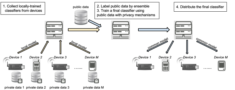
In this paper, we propose a method of building a global differentially private classifier from an ensemble of local classifier in two steps (see Fig. 1.) In the first step, locally-trained classifiers are collected by a trusted entity. A naive approach to use the collected classifiers is to release (the parameters of) the classifiers after sanitization by differentially private mechanisms, which is impractical (Sec. 3.2.) Instead, we use the classifier ensemble to generates (pseudo)labels for auxiliary unlabeled data, thus transferring the knowledge of the ensemble to the auxiliary data. In the second step, we use the labeled auxiliary data to find an empirical risk minimizer, and release a differentially private classifier using output perturbation (Chaudhuri et al., 2011).

When generating labels for auxiliary data using an ensemble of classifiers, majority voting is the simplest choice. However, we show quantitatively that a global classifier trained from majority-voted labels is highly sensitive to individual votes of local classifiers. Consequently, the final classifier after differentially-private sanitization suffer a heavy loss in its performance. To address this, we propose a new risk insensitive to individual votes, where each sample is weighted by the confidence of the ensemble. We provide an interpretation of the weighted risk in terms of random hypothesis of an ensemble (Breiman, 1996a) in contrast to deterministic labeling rule of majority voting. One of our main results is in Theorem 4: we can achieve $\epsilon$-differential privacy with a generalization error of $O(\epsilon^{-2}M^{-2})$ and $O(N^{-1})$ terms, relative to the expected risk of a non-private solution, where $M$ is the number of parties and $N$ is the number of samples in auxiliary data. This result is especially useful in a scenario where there are a large number of parties with weak local classifiers such as a group of connected smart devices with limited computing capability. We demonstrate the performance of our approach with several realistic tasks: activity recognition, network intrusion detection, and malicious URL detection. The results show that it is feasible to achieve both accuracy and privacy with a large number of parties.

To summarize, we propose a method of building a global differentially private classifier from locally-trained classifiers of multiple parties without access to their private data. The proposed method has the following advantages: 1) it can use local classifiers of any (mixed) types and therefore is flexible; 2) its generalization error converges to that of a non-private solution with a fast rate of $O(\epsilon^{-2}M^{-2})$ and $O(N^{-1})$; 3) it also provides $\epsilon$-differential privacy to all samples of a party and not just a single sample.

In Sec. 2, we formally describe privacy definitions. In Sec. 3, we discuss the first step of leveraging unlabeled data, and in Sec. 4, we present the second step of finding a global private classifier via empirical risk minimization in two different forms. In Sec. 5, we discuss related works. We evaluate the methods with real tasks in Sec. 6 and conclude the paper in Sec. 7. Appendix contains omitted proofs and several extensions of the algorithms.

2 Preliminary

2.1 Differential privacy

A randomized algorithm that takes data $\mathcal{D}$ as input and outputs a function $f$ is called $\epsilon$-differentially private if

$$\frac{P(f(\mathcal{D})\in\mathcal{S})}{P(f(\mathcal{D}^{\prime})\in\mathcal{S})}\leq e^{\epsilon}$$ (1)

for all measurable $\mathcal{S}\subset\mathcal{T}$ of the output range and for all datasets $\mathcal{D}$ and $\mathcal{D}^{\prime}$ differing in a single item, denoted by $\mathcal{D}\sim\mathcal{D}^{\prime}$. That is, even if an adversary knows the whole dataset $\mathcal{D}$ except for a single item, she cannot infer much about the unknown item from the output $f$ of the algorithm. When an algorithm outputs a real-valued vector $f\in\mathbb{R}^{D}$, its global $L_{2}$ sensitivity (Dwork et al., 2006) can be defined as

$$S(f)=\max_{\mathcal{D}\sim\mathcal{D}^{\prime}}\|f(\mathcal{D})-f(\mathcal{D}^{\prime})\|$$ (2)

where $\|\cdot\|$ is the $L_{2}$ norm. An important result from (Dwork et al., 2006) is that a vector-valued output $f$ with sensitivity $S(f)$ can be made $\epsilon$-differentially private by perturbing $f$ with an additive noise vector $\eta$ whose density is

$$P(\eta)\propto e^{-\frac{\epsilon}{S(f)}\|\eta\|}.$$ (3)

2.2 Output perturbation

When a classifier which minimizes empirical risk is released in public, it leaks information about the training data. Such a classifier can be sanitized by perturbation with additive noise calibrated to the sensitivity of the classifier, known as output perturbation method (Chaudhuri et al., 2011). Specifically, the authors show the following. If $w_{s}$ is the minimizer of the regularized empirical risk

$$R^{\lambda}_{S}(w)=\frac{1}{N}\sum_{(x,y)\in S}l(h(x;w),y)+\frac{\lambda}{2}\|w\|^{2},$$ (4)

Then the perturbed output $w_{p}=w_{s}+\eta,\;p(\eta)\propto e^{-\frac{N\lambda\epsilon}{2}\|\eta\|}$ is $\epsilon$-differentially private for a single sample. Output perturbation was used to sanitize the averaged parameters in (Pathak et al., 2010). We also use output perturbation to sanitize global classifiers. One important difference of our setting to previous work is that we consider $\epsilon$-differential privacy of all samples of a party, which is much stronger than $\epsilon$-differential privacy of a single sample.

There are conditions on the loss function for this guarantee to hold. We will assume the following conditions for our global classifier similar to (Chaudhuri et al., 2011).

• The loss-hypothesis has a form $l(h(x;w),v))=l(vw^{T}\phi(x))$, where $\phi:\mathcal{X}\to\mathbb{R}^{d}$ is a fixed map. We will consider only linear classifiers $l(vw^{T}x)$, where any nonlinear map $\phi$ is absorbed into the $d$-dimensional features.

• The surrogate loss $l(\cdot)$ is convex and continuously differentiable.

• The derivative $l^{\prime}(\cdot)$ is bounded: $|l^{\prime}(t)|\leq 1,\;\forall t\in\mathbb{R}$, and $c$-Lipschitz: $|l^{\prime}(s)-l^{\prime}(t)|\leq c|s-t|,\;\forall s,t\in\mathbb{R}.$

• The features are bounded: $\sup_{x\in\mathcal{X}}\|x\|\leq 1$.

These conditions are satisfied by, e.g., logistic regression loss ($c=1/4$) and approximate hinge loss.

3 Transferring knowledge of ensemble

3.1 Local classifiers

In this paper, we treat local classifiers as $M$ black boxes $h_{1}(x),...,h_{M}(x)$. We assume that a local classifier $h_{i}(x)$ is trained using its private i.i.d. training set $S^{(i)}$

$$S^{(i)}=\{(x^{(i)}_{1},y^{(i)}_{1}),\;...\;,(x^{(i)}_{N_{i}},y^{(i)}_{N_{i}})\},$$ (5)

where $(x^{(i)}_{j},y^{(i)}_{j})\in\mathcal{X}\times\{-1,1\}$ is a sample from a distribution $P(x,y)$ common to all parties. We consider binary labels $y\in\{-1,1\}$ in the main paper, and present a multiclass extension in Appendix B.

This splitting of training data across parties is similar to the Bagging procedure (Breiman, 1996a) with some differences. In Bagging, the training set $S^{(i)}$ for party $i$ is sampled with replacement from the whole dataset $\mathcal{D}$, whereas in our setting, the training set is sampled without replacement from $\mathcal{D}$, more similar to the Subagging (Politis et al., 1999) procedure.

3.2 Privacy issues of direct release

In the first step of our method, local classifiers from multiple parties are first collected by a trusted entity. A naive approach to use the ensemble is to directly release the local classifier parameters to the parties after appropriate sanitization. However, this is problematic in efficiency and privacy. Releasing all $M$ classifier parameters is an operation with a constant sensitivity, as opposed to releasing insensitive statistics such as an average whose sensitivity is $O(M^{-1})$. Releasing the classifiers requires much stronger perturbation than necessary, incurring steep loss of performance of sanitized classifiers. Besides, efficient differentially private mechanisms are known only for certain types of classifiers so far (see (Ji et al., 2014) for a review.) Another approach is to use the ensemble as a service to make predictions for test data followed by appropriate sanitization. Suppose we use majority voting to provide a prediction for a test sample. A differentially private mechanism such as Report Noisy Max (Dwork & Roth, 2013) can be used to sanitize the votes for a single query. However, answering several queries requires perturbing all answers with noise linearly proportional to the number of queries, which is impractical in most realistic settings.

3.3 Leveraging auxiliary data

To address the problems above, we propose to transfer the knowledge of the ensemble to a global classifier using auxiliary unlabeled data. More precisely, we use the ensemble to generate (pseudo)labels for the auxiliary data, which in turn are used to train a global classifier. Compared to directly releasing local classifiers, releasing a global classifier trained on auxiliary data is a much less sensitive operation with $O(M^{-1})$ (Sec. 4.4) analogous to releasing an average statistic. The number of auxiliary samples does not affect privacy, and in fact the larger the data the closer the global classifier is to the original ensemble with $O(N^{-1})$ bound (Sec. 4.4). Also, compared to using the ensemble to answer prediction queries, the sanitized global classifier can be used as many times as needed without its privacy being affected.

We argue that the availability of auxiliary unlabeled data is not an issue, since in many settings they are practically much easier to collect than labeled data. Furthermore, if the auxiliary data are obtained from public repositories, privacy of such data is not an immediate concern. We mainly focus on the privacy of local data, and discuss extensions for preserving the privacy of auxiliary data in Sec. 4.5.

4 Finding a global private classifier

We present details of training a global private classifier. As the first attempt, we use majority voting of an ensemble to assign labels to auxiliary data, and find a global classifier from the usual ERM procedure. In the second attempt, we present a better approach where we use the ensemble to estimate the posterior $P(y|x)$ of the auxiliary samples and solve a ‘soft-labeled’ weighted empirical minimization.

4.1 First attempt: ERM with majority voting

As the first attempt, we use majority voting of $M$ local classifiers to generate labels of auxiliary data, and analyze its implications. Majority voting for binary classification is the following rule

$$v(x)=\left\{\begin{array}[]{cc}1,&\mathrm{if}\;\;\;\sum_{i=1}^{M}I[h_{i}(x)=1]\geq\frac{M}{2}\\ -1,&\mathrm{otherwise}\end{array}\right..$$ (6)

Ties can be ignored by assuming an odd number $M$ of parties. Regardless of local classifier types or how they are trained, we can consider the majority vote of the ensemble $\{h_{1},...,h_{M}\}$ as a deterministic target concept to train a global classifier.

The majority-voted auxiliary data are

$$S=\{(x_{1},v(x_{1})),\;...,\;(x_{N},v(x_{N}))\},$$ (7)

where $x_{i}\in\mathcal{X}$ is an i.i.d. sample from the same distribution $P(x)$ as the private data. We train a global classifier by minimizing the (regularized) empirical risk associated with a loss and a hypothesis class:

$$R^{\lambda}_{S}(w)=\frac{1}{N}\sum_{(x,v)\in S}l(h(x;w),v)+\frac{\lambda}{2}\|w\|^{2}.$$ (8)

The corresponding expected risks with and without regularization are

$$R^{\lambda}(w)=E_{x}[l(h(x;w),v(x))]+\frac{\lambda}{2}\|w\|^{2},$$ (9)

and

$$R(w)=E_{x}[l(h(x;w),v(x))].$$ (10)

Algorithm 1 summarizes the procedure.

Algorithm 1 DP Ensemble by Majority-voted ERM

Input: $h_{1},...,h_{M}$ (local classifiers), $X$ (auxiliary unlabeled samples), $\epsilon$, $\lambda$
Output: $w_{p}$
Begin

  for $i=1,\;...\;,N$ do

     Generate majority voted labels $v(x_{i})$ by (6)

  end for

  Find the minimizer $w_{s}$ of (8) with $S=\{(x_{i},v(x_{i}))\}$

  Sample a random vector $\eta$ from $p(\eta)\propto e^{-0.5\lambda\epsilon\|\eta\|}$

  Output $w_{p}=w_{s}+\eta$

Applying output perturbation to our multiparty setting gives us the following result.

Theorem 1.

The perturbed output $w_{p}=w_{s}+\eta$ from Algorithm 1 with $p(\eta)\propto e^{-\frac{\lambda\epsilon}{2}\|\eta\|}$ is $\epsilon$-differentially private.

The proof of the theorem and others are in the Appendix A.

4.2 Performance issues of majority voting

We briefly discuss the generalization error of majority-voted ERM. In (Chaudhuri et al., 2011), it is shown that the expected risk of an output-perturbed ERM solution $w_{p}$ with respect to the risk of any reference hypothesis $w_{0}$ is bounded by two terms – one due to noise and another due to the gap between expected and empirical regularized risks. This result is applicable to the majority-voted ERM with minor modifications. The sensitivity of majority-voted ERM from Theorem 1 is $\frac{2}{\lambda}$ compared to $\frac{2}{N\lambda}$ of a standard ERM, and corresponding the error bound is

$$R(w_{p})\leq R(w_{0})+O(\epsilon^{-2})+O(N^{-1}),$$ (11)

with high probability, ignoring other variables. Unfortunately, the bound does not guarantee a successful learning due to the constant gap $O(\epsilon^{-2})$, which can be large for a small $\epsilon$.

What causes this is the worst-case scenario of multiparty voting. Suppose the votes of $M-1$ local classifiers are exactly ties for all auxiliary samples $\{x_{1},...,x_{N}\}$. If we replace a local classifier $h_{i}(x)$ with the ‘opposite’ classifier $h_{i}^{\prime}(x)=-h_{i}(x)$, then the majority-voted labels $\{v_{1},...,v_{N}\}$ become $\{-v_{1},...,-v_{N}\}$, and the resultant global classifier is entirely different. However unlikely this scenario may be in reality, differential privacy requires that we calibrate our noise to the worst case sensitivity.

4.3 Better yet: weighted ERM with soft labels

The main problem with majority voting was its sensitivity to the decision of a single party. Let $\alpha(x)$ be the fraction of positive votes from $M$ classifiers given a sample $x$:

$$\alpha(x)=\frac{1}{M}\sum_{j=1}^{M}I[h_{j}(x)=1].$$ (12)

In terms of $\alpha$, the original loss $l(w^{T}xv(x))$ for majority voting can be written as

$$l(yw^{T}x) = I[\alpha(x)\geq 0.5]\;l(w^{T}x)$$ (13)

$$\;\;+\;\;I[\alpha(x)<0.5]\;l(-w^{T}x),$$

which changes abruptly when the fraction $\alpha(x)$ crosses the boundary $\alpha=0.5$. We remedy the situation by introducing the new weighted loss:

$$l^{\alpha}(\cdot)=\alpha(x)l(w^{T}x)+(1-\alpha(x))l(-w^{T}x).$$ (14)

The new loss has the following properties. When the $M$ votes given a sample $x$ are unanimously positive (or negative), then the weighted loss is $l^{\alpha}(\cdot)=l(w^{T}x)$ (or $l(-w^{T}x)$), same as the original loss. If the votes are almost evenly split between positive and negative, then the weighted loss is $l^{\alpha}(\cdot)\simeq 0.5\;l(w^{T}x)+0.5\;l(-w^{T}x)$ which is insensitive to the change of label by a single vote, unlike the original loss. Specifically, a single vote can change $l^{\alpha}(\cdot)$ only by a factor of $1/M$ (see Proof of Theorem 3.)

We provide a natural interpretation of $\alpha(x)$ and the weighted loss in the following. For the purpose of analysis, assume that the local classifiers $h_{1}(x),...,h_{M}(x)$ are from the same hypothesis class. Since the local training data are i.i.d. samples from $P(x,y)$, the local classifiers $\{h_{1}(x),...,h_{M}(x)\}$ can be considered random hypotheses, as in (Breiman, 1996a). Let $Q(j|x)$ be the probability of such a random hypothesis $h(x)$ predicting label $j$ given $x$:

$$Q(j|x)=P(h(x)=j|x),$$ (15)

Then the fraction $\alpha(x)=\frac{1}{M}\sum_{j=1}^{M}I[h_{j}(x)=1]$ is an unbiased estimate of $Q(1|x)$. Furthermore, the weighted loss is directly related to the unweighted loss:

Lemma 2.

For any $w$, the expectation of the weighted loss (14) is asymptotically the expectation of the unweighted loss:

$$\lim_{M\to\infty}E_{x}[l^{\alpha}(w)]=E_{x,v}[l(w^{T}xv)].$$ (16)

Proof.

The expected risk $E_{x,v}[l(vw^{T}x)]$ is

$$= E_{x}E_{v|x}[l(vw^{T}x)]$$ (17)

$$= E_{x}[Q(1|x)l(w^{T}x)+Q(-1|x)l(-w^{T}x)]$$

$$= E_{x}[\lim_{M\to\infty}\alpha(x)l(w^{T}x)+(1-\lim_{M\to\infty}\alpha(x))l(-w^{T}x)]$$

$$\;\;\;(\mathrm{the\;law\;of\;large\;numbers})$$

$$= \lim_{M\to\infty}E_{x}[\alpha(x)l(w^{T}x)+(1-\alpha(x))l(-w^{T}x)]$$

$$\;\;\;(\mathrm{bounded}\;\alpha\;\mathrm{and}\;l\;\mathrm{for}\;\forall x\in\mathcal{X})$$

$$= \lim_{M\to\infty}E_{x}[l^{\alpha}(w)].$$

∎

This shows that minimizing the expected weighted loss is asymptotically the same as minimizing the standard expected loss, when the target $v$ is a probabilistic concept from $P(h(x)=v)$ of the random hypothesis, as opposed to a deterministic concept $v(x)$ from majority voting.

The auxiliary dataset with ‘soft’ labels is now

$$S=\{(x_{1},\alpha(x_{1})),\;...\;,(x_{N},\alpha(x_{N}))\}.$$ (18)

where $x_{i}\in\mathcal{X}$ is an i.i.d. sample from the same distribution $P(x)$ as the private data, and $0\leq\alpha\leq 1$. Note that we are not trying to learn a regression function $\mathcal{X}\to[0,1]$ but to learn a classifier $\mathcal{X}\to\{-1,1\}$ using $\alpha$ as a real-valued oracle on $P(y=1|x)$. Consequently, we find a global classifier by minimizing the regularized weighted empirical risk

$$R^{\lambda}_{S}(w)=\frac{1}{N}\sum_{i=1}^{N}l^{\alpha}(h(x_{i};w),\alpha_{i})+\frac{\lambda}{2}\|w\|^{2},$$ (19)

where $\alpha_{i}=\alpha(x_{i})$. The corresponding expected risks with and without regularization are

$$R^{\lambda}(w)=E_{x}[l^{\alpha}(h(x;w),\alpha(x))]+\frac{\lambda}{2}\|w\|^{2},$$ (20)

and

$$R(w)=E_{x}[l^{\alpha}(h(x;w),\alpha(x))].$$ (21)

We again use output perturbation to make the classifier differentially private as summarized in Algorithm 2.

Algorithm 2 DP Ensemble by Weighted ERM

Input: $h_{1},...,h_{M}$ (local classifiers), $X$ (auxiliary unlabeled samples), $\epsilon$, $\lambda$
Output: $w_{p}$
Begin

  for $i=1,\;...\;,N$ do

     Compute $\alpha(x_{i})$ by (12)

  end for

  Find the minimizer of $w_{s}$ of (19) with $\{(x_{i},\alpha(x_{i}))\}$

  Sample a random vector $\eta$ from $p(\eta)\propto e^{-0.5M\lambda\epsilon\|\eta\|}$

  Output $w_{p}=w_{s}+\eta$

4.4 Privacy and performance

Compared to Theorem 1 for majority-voted ERM with a noise of $P(\eta)\propto e^{-\frac{\lambda\epsilon}{2}\|\eta\|}$, we have the following result:

Theorem 3.

The perturbed output $w_{p}=w_{s}+\eta$ from Algorithm 2 with $p(\eta)\propto e^{-\frac{M\lambda\epsilon}{2}\|\eta\|}$ is $\epsilon$-differentially private.

That is, we now require $1/M$ times smaller noise to achieve the same $\epsilon$-differential privacy. This directly impacts the performance of the corresponding global classifier as follows.

Theorem 4.

Let $w_{0}$ be any reference hypothesis. Then with probability of at least $1-\delta_{p}-\delta_{s}$ over the privacy mechanism $(\delta_{p})$ and over the choice of samples $(\delta_{s})$,

$$R(w_{p}) \leq R(w_{0})+\frac{4d^{2}(c+\lambda)\log^{2}(d/\delta_{p})}{\lambda^{2}M^{2}\epsilon^{2}}$$ (22)

$$+\frac{16(32+\log(1/\delta_{s}))}{\lambda N}+\frac{\lambda}{2}\|w_{0}\|^{2}.$$

The generalization error bound above has the $O(M^{-2}\epsilon^{-2})$ term compared to the $O(\epsilon^{-2})$ term for majority-voted ERM (11). This implies that by choosing a large $M$, Algorithm 2 can find a solution whose expected risk is close to the minimum of a non-private solution for any fixed privacy level $\epsilon>0$.

We remind the user that the results should be interpreted with a caution. The bounds in (11) and (22) indicate the goodness of private ERM solutions relative to the best non-private solutions with deterministic and probability concepts which are not the same task. Also, they do not indicate the goodness of the ensemble approach itself relative to a centrally-trained classifier using all private data without privacy consideration. We leave this comparison to empirical evaluation in the experiment section.

4.5 Extensions

We discuss extensions of Algorithms 1 and  2 to provide additional privacy for auxiliary data. More precisely, those algorithms can be made $\epsilon$-differentially private for all private data of a single party and a single sample in the auxiliary data, by increasing the amount of perturbation as necessary. We outline the proof as follows. In the previous sections, a global classifier was trained on auxiliary data whose labels were generated either by majority voting or soft labeling. A change in the local classifier affects only the labels $\{v_{i}\}$ of the auxiliary data but not the features $\{x_{i}\}$. Now assume in addition that the feature of one sample from the auxiliary data can also change arbitrarily, i.e., $x_{j}\neq x^{\prime}_{j}$ for some $j$ and $x_{i}=x^{\prime}_{i}$ for all $i\in\{1,...,N\}\setminus\{j\}$. The sensitivity of the resultant risk minimizer can be computed similarly to the proofs of Theorems 1 and 3 in Appendix A. Briefly, the sensitivity is upper-bounded by the absolute sum of the difference of gradients

$$\|\nabla g(w)\|\leq\frac{1}{N}\sum_{i=1}^{N}\|\nabla l(y_{i}w^{T}x_{i})-\nabla l(y_{i}^{\prime}w^{T}x_{i}^{\prime})\|.$$ (23)

For majority voting, one term in the sum (23) is

$$\|v(x_{j})x_{j}l^{\prime}(v(x_{j})w^{T}x_{j})-v^{\prime}(x^{\prime}_{j})x^{\prime}_{j}l^{\prime}(v^{\prime}(x^{\prime}_{j})w^{T}x^{\prime}_{j})\|$$ (24)

which is at most 2 for any $x_{j},x_{j}^{\prime}\in\mathcal{X}$, and therefore the sensitivity is the same whether $x_{j}=x^{\prime}_{j}$ or not. As a result, Algorithm 1 is already $\epsilon$-differentially private for both labeled and auxiliary data without modification. Furthermore, the privacy guarantee remains the same if we allow $x_{j}\neq x^{\prime}_{j}$ for any number of samples. For soft labeling, one term in the sum (23) is

$$\|\alpha_{j}x_{j}l^{\prime}(w^{T}x_{j})-(1-\alpha_{j})x_{j}l^{\prime}(-w^{T}x_{j})$$

$$-\alpha^{\prime}_{j}x_{j}^{\prime}l^{\prime}(w^{T}x^{\prime}_{j})+(1-\alpha^{\prime}_{j})x^{\prime}_{j}l^{\prime}(-w^{T}x^{\prime}_{j})\|$$ (25)

which is also at most 2 for any $x_{j},x_{j}^{\prime}\in\mathcal{X}$ and $\frac{2}{M}$ when $x_{j}=x_{j}^{\prime}$. When only a single auxiliary sample changes, i.e., $x_{j}\neq x_{j}^{\prime}$ for one $j$, the overall sensitivity increases by a factor of $\frac{N+M-1}{N}$. By increasing the noise by this factor, Algorithm 2 is $\epsilon$-differentially private for both labeled and auxiliary data. Note that this factor $\frac{N+M-1}{N}$ can be bounded close to 1 if we increase the number of auxiliary samples $N$ relative to the number of parties $M$.

5 Related work

To preserve privacy in data publishing, several approaches such as $k$-anonymity (Sweeney, 2002) and secure multiparty computation (Yao, 1982) have been proposed (see (Fung et al., 2010) for a review.) Recently, differential privacy (Dwork & Nissim, 2004; Dwork et al., 2006; Dwork, 2006) has addressed several weaknesses of $k$-anonymity (Ganta et al., 2008), and gained popularity as a quantifiable measure of privacy risk. The measure provides a bound on the privacy loss regardless of any additional information an adversary might have. Differential privacy has been used for a privacy-preserving data analysis platform (McSherry, 2009), and for sanitization of learned model parameters from a standard ERM (Chaudhuri et al., 2011). This paper adopts output perturbation techniques from the latter to sanitize non-standard ERM solutions from multiparty settings.

Private learning from multiparty data has been studied previously. In particular, several differentially-private algorithms were proposed, including parameter averaging through secure multiparty computation (Pathak et al., 2010), and private exchange of gradient information to minimize empirical risks incrementally (Rajkumar & Agarwal, 2012; Hamm et al., 2015). Our paper is motivated by (Pathak et al., 2010) but uses a very different approach to aggregate local classifiers. In particular, we use an ensemble approach and average the classifier decisions (Breiman, 1996a) instead of parameters, which makes our approach applicable to arbitrary and mixed classifier types. Advantages of ensemble approaches in general have been analyzed previously, in terms of bias-variance decomposition (Breiman, 1996b), and in terms of the margin of training samples (Schapire et al., 1998).

Furthermore, we are using unlabeled data to augment labeled data during training, which can be considered a semi-supervised learning method (Chapelle et al., 2006). There are several related papers in this direction. Augmenting private data with non-private labeled data to lower the sensitivity of the output is straightforward, and was demonstrated in medical applications (Ji et al., 2014). Using non-private unlabeled data, which is more general than using labeled data, was demonstrated specifically to assist learning of random forests (Jagannathan et al., 2013). Our use of auxiliary data is not specific to classifier types. Furthermore, we present an extension to preserve the privacy of auxiliary data as well.

6 Experiments

We use three real-world datasets to compare the performance of the following algorithms:

• batch: classifier trained using all data ignoring privacy

• soft: private ensemble using soft-labels (Algorithm 2)

• avg: parameter averaging (Pathak et al., 2010)

• vote: private ensemble using majority voting (Algorithm 1)

• indiv: individually trained classifier using local data

We can expect batch to perform better than any private algorithm since it uses all private data for training ignoring privacy. In contrast, indiv uses only the local data for training and will perform significantly worse than batch, but it achieves a perfect privacy as long as the trained classifiers are kept local to the parties. We are interested in the range of $\epsilon$ where private algorithms (soft, avg, and vote) perform better than the baseline indiv.

To compare all algorithms fairly, we use only a single type of classier – binary or multiclass logistic regression. For Algorithms 1 and 2, both local and global classifiers are of this type as well. The only hyperparameter of the model is the regularization coefficient $\lambda$ which we fixed to $10^{-4}$ after performing some preliminary experiments.About $10\%$ of the original training data are used as auxiliary unlabeled data, and the rest $90\%$ are randomly distributed to $M$ parties as private data. We report the mean and s.d. over 10 trials for non-private algorithms and 100-trials for private algorithms.

Figure 2: Test accuracy of private and non-private algorithms for activity recognition with $K=6$ activity types.

Figure 3: Test accuracy of private and non-private algorithms for network intrusion detection.

Figure 4: Test accuracy of private and non-private algorithms for malicious URL detection.

6.1 Activity recognition using accelerometer

Consider a scenario where wearable device users want to train a motion-based activity classifier without revealing her data to others. To test the algorithms, we use the UCI Human Activity Recognition Dataset (Anguita et al., 2012), which is a collection of motion sensor data on a smart device by multiple subjects performing $6$ activities (walking, walking upstairs, walking downstairs, sitting, standing, laying). Various time and frequency domain variables are extracted from the signal, and we apply PCA to get $d=50$ dimensional features. The training and testing samples are $7K$ and $3K$, respectively.

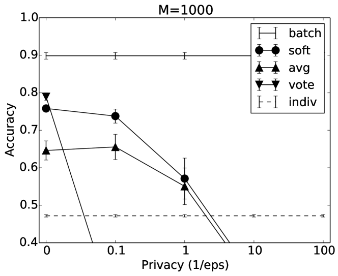
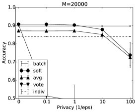
We simulate a case with $M=1K$ users (i.e., parties). Each user can use only $6$ samples to train a local classifier. The remaining $1K$ samples are used as auxiliary unlabeled data. Figure 2 shows the test accuracy of using different algorithms with varying privacy levels. For non-private algorithms, the top solid line (batch) shows the accuracy of a batch-trained classifier at around $0.90$, and the bottom dashed line (indiv) shows the averaged accuracy of local classifiers at around $0.47$. At $1/\epsilon=0$, the private algorithms achieve test accuracy of 0.79 (vote), 0.76 (soft) and 0.67 (avg), and as the the privacy level $1/\epsilon$ increases, the performance drops for all private algorithms. As expected from the bound (11), vote becomes useless even at $1/\epsilon=0.1$, while soft and avg are better than indiv until $1/\epsilon=1$. We fixed $M$ to 1000 in this experiment due to the limited number of samples, the tendency in the graph is similar to other experiments with larger $M$’s.

6.2 Network intrusion detection

Consider a scenario where multiple gateways or routers collect suspicious network activities independently, and aim to collaboratively build an accurate network intrusion detector without revealing local traffic data. For this task we use the KDD-99 dataset, which consists of examples of ‘bad’ connections, called intrusions or attacks, and ‘good’ normal connections. Features of this dataset consists of continuous values and categorical attributes. To apply logistic regression, we change categorical attributes to one-hot vectors to get $d=123$ dimensional features. The training and testing samples are $493K$ and $311K$, respectively.

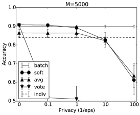
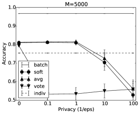
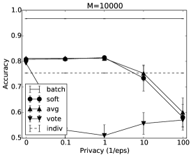
We simulate cases with $M=5K/10K/20K$ parties. Each party can only use $22$ samples to train a local classifier. The remaining $43K$ samples are used as auxiliary unlabeled data. Figure 3 shows the test accuracy of using different algorithms with varying privacy levels. For each of $M=5K/10K/20K$ the tendency of algorithms is similar to Figure 2 – for a small $1/\epsilon$, private algorithms perform roughly in between batch and indiv, and as $1/\epsilon$ increases private algorithms start to perform worse than indiv. When $M$ is large (e.g., $M=20K$), private algorithms soft and avg hold their accuracy better than when $M$ is small (e.g., $M=5K$.) In particular, soft performs nearly as well as the non-private batch until around $1/\epsilon=10$ compared to ${\it avg}$.

6.3 Malicious URL prediction

In addition to network intrusion detection, multiple parties such as computer users can collaborate on detecting malicious URLs without revealing the visited URLs. The Malicious URL Dataset (Ma et al., 2009) is a collection of examples of malicious URLs from a large Web mail provider. The task is to predict whether a URL is malicious or not by various lexical and host-based features of the URL. We apply PCA to get $d=50$ dimensional feature vectors. We choose days 0 to 9 for training, and days 10 to 19 for testing, which amount to $200K$ samples for training and $200K$ samples for testing.

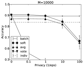
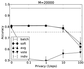
We simulate cases with $M=5K/10K/20K$ parties. Each party can use only $9$ samples to train a local classifier. The remaining $16K$ samples are used as auxiliary unlabeled data. Figure 4 shows the test accuracy of using different algorithms with varying privacy levels. The gap between batch and other algorithms is larger compared to the previous experiment (Figure 3), most likely due to the smaller number (=9) of samples per party. However, the overall tendency is very similar to previous experiments.

7 Conclusion

In this paper, we propose a method of building global differentially private classifiers from local classifiers using two new ideas: 1) leveraging unlabeled auxiliary data to transfer the knowledge of the ensemble, and 2) solving a weighted ERM using class probability estimates from the ensemble. In general, privacy comes with a loss of classification performance. We present a solution to minimize the performance gap between private and non-private ensembles demonstrated with real world tasks.

Appendix A Proofs

A.1 Proof of Theorem 1

Theorem 1: The perturbed output $w_{p}=w_{s}+\eta$ from Algorithm 1 with $p(\eta)\propto e^{-\frac{\lambda\epsilon}{2}\|\eta\|}$ is $\epsilon$-differentially private.

Proof.

We will compute the sensitivity of the minimizer $w_{s}$ of the regularized empirical risk with majority-voted labels (8). Suppose $\mathcal{D}=(S^{(1)},...,S^{(M)})$ is the ordered set of private training data (5) for $M$ parties, and $\mathcal{D}^{\prime}=((S^{\prime})^{(1)},...,S^{(M)})$ is a neighboring set which differs from $\mathcal{D}$ only at party 1’s data, without loss of generality. The local classifiers after training with $\mathcal{D}$ and $\mathcal{D}^{\prime}$ are $H=(h_{1},...,h_{M})$ and $H^{\prime}=(h_{1}^{\prime},...,h_{M})$, respectively, which are again different only for classifier 1. The majority votes $v(x)$ and $v^{\prime}(x)$ from $\mathcal{D}$ and $\mathcal{D}^{\prime}$ generates two auxiliary training sets $S=\{(x_{i},v(x_{i}))\}$ and $S^{\prime}=\{(x_{i},v^{\prime}(x_{i})\}$ which have the same features but possibly different labels.

Let $R^{\lambda}_{S}(w)$ and $R^{\lambda}_{S^{\prime}}(w)$ be the regularized empirical risks for training sets $S$ and $S^{\prime}$, and let $w_{s}$ and $w_{s^{\prime}}$ be the minimizers of the respective risks. From Corollaries 7 and 8 (Chaudhuri et al., 2011), the $L_{2}$ difference of $w_{s}$ and $w_{s^{\prime}}$ is bounded by

$$\|w_{s}-w_{s^{\prime}}\|\leq\frac{1}{\lambda}\max_{w}\|\nabla g(w)\|,$$ (26)

where $g(w)$ is the risk difference $R^{\lambda}_{S}(w)-R^{\lambda}_{S^{\prime}}(w)$, which, in our case, satisfies

$$\|\nabla g(w)\| \leq \frac{1}{N}\sum_{i=1}^{N}\|v(x_{i})x_{i}l^{\prime}(v(x_{i})w^{T}x_{i})$$ (27)

$$\;\;-v^{\prime}(x_{i})x_{i}l^{\prime}(v^{\prime}(x_{i})w^{T}x_{i})\|.$$

$$\leq \frac{1}{N}\sum_{i=1}^{N}\|x_{i}\|\times$$

$$|l^{\prime}(w^{T}x_{i})+l^{\prime}(-w^{T}x_{i})|.$$

Recall that $\|x\|\leq 1$ and $|l^{\prime}(\cdot)|\leq 1$ by assumption. In the worst case, $v(x_{i})\neq v^{\prime}(x_{i})$ for all $i=1,...,N$, and therefore the RHS of (27) is bounded by 2. Consequently, the $L_{2}$ sensitivity of the minimizer $w_{s}$ is

$$\max_{S,S^{\prime}}\|w_{s}-w_{s^{\prime}}\|\leq\frac{2}{\lambda}.$$ (28)

$\epsilon$-differential privacy follows from the sensitivity result (3). ∎

A.2 Proof of Theorem 3

Theorem 3: The perturbed output $w_{p}=w_{s}+\eta$ from Algorithm 2 with $p(\eta)\propto e^{-\frac{M\lambda\epsilon}{2}\|\eta\|}$ is $\epsilon$-differentially private.

Proof.

The proof parallels the proof of Theorem 1. We again assume $\mathcal{D}=(S^{(1)},...,S^{(M)})$ is the ordered set of private training data (5) for $M$ parties, and $\mathcal{D}^{\prime}=((S^{\prime})^{(1)},...,S^{(M)})$ is a neighboring set which differs from $\mathcal{D}$ only at party 1’s data, without loss of generality. Let $S=\{(x_{i},\alpha_{i})\}$ and $S^{\prime}=\{(x_{i},\alpha^{\prime}_{i})\}$ be the two resulting datasets which have the same the features but possibly different $\alpha$’s. We first compute the sensitivity of the minimizer of the weighted regularized empirical risk (19). Let $R^{\lambda}_{S}(w)$ and $R^{\lambda}_{S^{\prime}}(w)$ be the regularized empirical risks for training sets $S$ and $S^{\prime}$, and let $w_{s}$ and $w_{s^{\prime}}$ be the minimizers of the respective risks. Also let $g(w)$ be the difference $R^{\lambda}_{S}(w)-R^{\lambda}_{S^{\prime}}(w)$ of two risks

$$g(w) = \frac{1}{N}\sum_{i=1}^{N}[\alpha_{i}l(w^{T}x_{i})+(1-\alpha_{i})l(-w^{T}x_{i})$$ (29)

$$-\alpha^{\prime}_{i}l(w^{T}x_{i})-(1-\alpha^{\prime}_{i})l(-w^{T}x_{i})].$$

The gradient of $g(w)$ is bounded by

$$\|\nabla g(w)\| \leq \frac{1}{N}\sum_{i=1}^{N}[|\alpha_{i}-\alpha^{\prime}_{i}|\|x_{i}\||l^{\prime}(w^{T}x_{i})|$$ (30)

$$+|\alpha_{i}-\alpha^{\prime}_{i}|\|x_{i}\||l^{\prime}(-w^{T}x_{i})|]$$

$$\leq \frac{1}{N}\sum_{i=1}^{N}2|\alpha_{i}-\alpha^{\prime}_{i}|.$$ (31)

In the worst case, $\alpha_{i}\neq\alpha_{i}^{\prime}$ for all $i=1,...,N$. Since $\alpha_{i}$ is the fraction of positive votes, $|\alpha_{i}-\alpha_{i}^{\prime}|\leq 1/M$ holds for all $i=1,...,N$. Therefore the $L_{2}$ sensitivity of the minimizer $w_{s}$ is at most $\frac{2}{\lambda M}$ and the $\epsilon$-differential privacy follows. ∎

A.3 Lemma 5

We use the following lemma.

Lemma 5 (Lemma 17 of (Chaudhuri et al., 2011)).

If $X\sim\Gamma(k,\theta)$, where $k$ is an integer, then with probability of at least $1-\delta$,

$$X\leq k\theta\log(k/\delta).$$

A.4 Lemma 6

Lemma 6.

If $w_{s}$ is the minimizer of (19) and $w_{p}$ is the $\epsilon$-differentially private version from Algorithm 2, then with probability of at least $1-\delta_{p}$ over the privacy mechanism,

$$R^{\lambda}_{S}(w_{p})\leq R^{\lambda}_{S}(w_{s})+\frac{2d^{2}(c+\lambda)\log^{2}(d/\delta)}{\lambda^{2}M^{2}\epsilon^{2}}$$ (32)

Proof.

A differentiable function $f:\mathbb{R}^{d}\to\mathbb{R}$ is called $\beta$-smooth, if $\exists\beta>0$ such that $\|\nabla f(v)-\nabla f(u)\|\leq\beta\|v-u\|$ for all $u,v$. From the Mean Value Theorem, such a function satisfies

$$f(v)\leq f(u)+\nabla^{T}f(u)(v-u)+\frac{\beta}{2}\|v-u\|^{2},\;\forall u,v.$$

Since $|l^{\prime}(\cdot)|$ is $c$-Lipschitz, $R^{\lambda}_{S}(w)$ is $(c+\lambda)$-smooth:

$$\|\nabla R^{\lambda}_{S}(v)-\nabla R^{\lambda}_{S}(u)\|$$

$$\leq\frac{1}{N}\sum_{i}\left\|\alpha_{i}x_{i}l^{\prime}(v^{T}x_{i})-(1-\alpha_{i})x_{i}l^{\prime}(-v^{T}x_{i})\right.$$

$$\left.-\alpha_{i}x_{i}l^{\prime}(u^{T}x_{i})+(1-\alpha_{i})x_{i}l^{\prime}(-u^{T}x_{i})\right\|$$

$$+\lambda\|v-u\|$$

$$\leq\frac{1}{N}\sum_{i}\left[\alpha_{i}c\|(v-u)^{T}x_{i}\|+\right.$$

$$\left.(1-\alpha_{i})c\|(u-v)^{T}x_{i}\|\right]+\lambda\|v-u\|$$

$$\leq(c+\lambda)\|u-v\|.$$ (33)

By setting $v=w_{p}$ and $u=w_{s}$ and using the $(c+\lambda)$-smoothness of $R^{\lambda}_{S}(w)$, we have

$$R^{\lambda}_{S}(w_{p}) \leq R^{\lambda}_{S}(w_{s})+\nabla^{T}R^{\lambda}_{S}(w_{s})(w_{p}-w_{s})$$ (34)

$$\;\;\;+\frac{(c+\lambda)}{2}\|w_{p}-w_{s}^{\ast}\|^{2}$$

$$= R^{\lambda}_{S}(w_{s})+\frac{(c+\lambda)}{2}\|w_{p}-w_{s}\|^{2}.$$

Since

$$P\left(\|w_{p}-w_{s}^{\ast}\|\leq\frac{2d\log(d/\delta)}{\lambda M\epsilon}\right)\geq 1-\delta_{p}$$ (35)

from Lemma 5 with $k=d$ and $\theta=\frac{2}{\lambda M\epsilon}$, we have the desired result. ∎

A.5 Proof of Theorem 4

Theorem 4: Let $w_{0}$ be any reference hypothesis. Then with probability of at least $1-\delta_{p}-\delta_{s}$ over the privacy mechanism $(\delta_{p})$ and over the choice of samples $(\delta_{s})$,

$$R(w_{p}) \leq R(w_{0})+\frac{4d^{2}(c+\lambda)\log^{2}(d/\delta_{p})}{\lambda^{2}M^{2}\epsilon^{2}}$$ (36)

$$+\frac{16(32+\log(1/\delta_{s}))}{\lambda N}+\frac{\lambda}{2}\|w_{0}\|^{2}.$$

Proof.

Let $w_{s}$ and $w^{\ast}$ be the minimizers of the regularized empirical risk (19) and the regularized expected risk (20), respectively. The risk at $w_{p}$ relative to a reference classifier $w_{0}$ can be written as

$$R(w_{p})-R(w_{0}) = R^{\lambda}(w_{p})-R^{\lambda}(w^{\ast})$$

$$+R^{\lambda}(w^{\ast})-R^{\lambda}(w_{0})$$

$$+\frac{\lambda}{2}\|w_{0}\|^{2}-\frac{\lambda}{2}\|w_{p}\|^{2}$$

$$\leq R^{\lambda}(w_{p})-R^{\lambda}(w^{\ast})+\frac{\lambda}{2}\|w_{0}\|^{2}.$$

The inequality above follows from $R^{\lambda}(w^{\ast})\leq R^{\lambda}(w_{0})$ by definition. Note that since $\|x\|\leq 1$ and $|l^{\prime}|\leq 1$ by assumption, the weighted loss $\alpha(x)l(w^{T}x)+(1-\alpha(x))l(w^{T}x)$ is $1$-Lipschitz in $w$. From Theorem 1 of (Sridharan et al., 2009) with $a=1$, we can also bound $R^{\lambda}(w_{p})-R^{\lambda}(w^{\ast})$ as

$$R^{\lambda}(w_{p})-R^{\lambda}(w^{\ast}) \leq 2(R^{\lambda}_{S}(w_{p})-R^{\lambda}_{S}(w_{s}^{\ast}))$$ (38)

$$+\frac{16(32+\log(1/\delta_{s}))}{\lambda N}$$

with probability of $1-\delta_{s}$ over the choice of samples. By combining this inequality with Lemma 6 using the union bound, we have

$$R^{\lambda}(w_{p})-R^{\lambda}(w^{\ast}) \leq \frac{4d^{2}(c+\lambda)\log^{2}(d/\delta_{p})}{\lambda^{2}M^{2}\epsilon^{2}}$$ (39)

$$+\frac{16(32+\log(1/\delta_{s}))}{\lambda N}.$$

The theorem follows from (LABEL:eq:thm5_ineq).

∎

Appendix B Differentially private multiclass logistic regression

We extend our methods to multiclass classification problems and provide a sketch of $\epsilon$-differential privacy proofs for multiclass logistic regression loss.

B.1 Standard ERM

Suppose $y\in 1,...,K$, and let $w=[w_{1};\;...\;;w_{K}]$ be a stacked $(d\;K)\times 1$ vector. The multiclass logistic loss (i.e. softmax) is

$$l(h(x),y)=-w_{y}^{T}x+\log(\sum_{l}e^{w_{l}^{T}x}),$$ (40)

and the regularized empirical risk is

$$R^{\lambda}_{S}(w)=-\frac{1}{N}\sum_{i}[w_{y_{i}}^{T}x_{i}-\log(\sum_{l}e^{w_{l}^{T}x_{i}})]+\frac{\lambda}{2}\|w\|^{2}.$$ (41)

Note that $R^{\lambda}_{S}(w)$ is $\lambda$-strongly convex in $w$.

The sensitivity of $w_{s}$ which minimizes (41) can be computed as follows. Suppose $S$ and $S^{\prime}$ are two different datasets which are not necessarily neighbors: $S=\{(x_{i},y_{i}))\}$ and $S^{\prime}=\{(x^{\prime}_{i},y^{\prime}_{i})\}$. Let $g(w)$ be the difference $R^{\lambda}_{S}(w)-R^{\lambda}_{S^{\prime}}(w)$ of the two risks. Then the partial gradient w.r.t. $w_{k}$ is

$$\nabla_{w_{k}}R^{\lambda}_{S}(w)=-\frac{1}{N}\sum_{i}x_{i}\Delta_{k}(x_{i},y_{i},w)+\lambda w_{k},$$ (42)

where

$$\Delta_{k}(x_{i},y_{i},w)=I[y_{i}=k]-\frac{e^{w_{k}^{T}x_{i}}}{\sum_{l}e^{w_{l}^{T}x_{i}}}=I[y_{i}=k]-P_{k}(x_{i}).$$ (43)

Since $I[y_{i}=k]$ can be non-zero (i.e. 1) for only one $k$, and $\sum_{k}P_{k}(x_{i})=1$ with $0\leq P_{k}(x_{i})\leq 1$, we have

$$\sum_{k}\Delta_{k}^{2}=\sum_{k}(I_{k}-P_{k})^{2}\leq\sum_{k}(I_{k}^{2}+P_{k}^{2})\leq 2,$$ (44)

Let $\Delta(x_{i},y_{i},w)=[\Delta_{1}(x_{i},y_{i},w),...,\Delta_{K}(x_{i},y_{i},w)]$ be a $K\times 1$ vector (which depends on $x_{i},y_{i},w$.) The gradient of the risk difference $g(w)$ is then

$$\nabla g(w)=-\frac{1}{N}\sum_{i}\Delta(x_{i},y_{i},w)\otimes x_{i}-\Delta(x_{i}^{\prime},y_{i}^{\prime},w)\otimes x_{i}^{\prime},$$ (45)

where $\otimes$ is a Kronecker product of two vectors. Note that

$$\|\Delta\otimes x\|^{2}=\sum_{k}\|\Delta_{k}x\|^{2}\leq\|x\|^{2}\sum_{k}\Delta_{k}^{2}\leq 2\|x\|^{2}.$$ (46)

Without loss of generality, we assume that only $(x_{1},y_{1})$ and $(x^{\prime}_{1},y^{\prime}_{1})$ are possibly different and $(x_{i},y_{i})=(x_{i}^{\prime},y_{i}^{\prime})$ for all $i=2,...,N$. In this case we have

$$\|\nabla g(w)\| \leq \frac{1}{N}\|\Delta(x_{1},y_{1},w)\otimes x_{1}\|$$ (47)

$$+\frac{1}{N}\|\Delta(x^{\prime}_{1},y^{\prime}_{1},w)\otimes x^{\prime}_{1}\|$$

$$\leq \frac{\sqrt{2}}{N}(\|x_{1}\|+\|x^{\prime}_{1}\|)\leq\frac{2\sqrt{2}}{N},$$

and the therefore the $L_{2}$ sensitive of the minimizer of a multiclass logistic regression is

$$\frac{2\sqrt{2}}{N\lambda}$$ (48)

from Corollaries 7 and 8 (Chaudhuri et al., 2011). Note that the sensitivity does not depend on the number of classes $K$.

B.2 Majority-voted ERM

Let $S=\{(x_{i},v_{i})\}$ and $S^{\prime}=\{(x_{i},v_{i}^{\prime})\}$ be two datasets with the same features but with possibly different labels for all $i=1,...,N$. Then the partial gradient of the risk difference $g(w)$ is

$$\nabla_{w_{k}}g(w) = -\frac{1}{N}\sum_{i}x_{i}[I[v_{i}=k]-I[v^{\prime}_{i}=k]]$$ (49)

$$= -\frac{1}{N}\sum_{i}x_{i}a_{k}(v_{i},v_{i}^{\prime}),$$

where $a_{k}(v_{i},v_{i}^{\prime})$ is

$$a_{k}(v_{i},v^{\prime}_{i})=I[v_{i}=k]-I[v^{\prime}_{i}=k]\in\{-1,0,1\}.$$ (50)

Let $a=[a_{1},...,a_{K}]$ be a $K\times 1$ vector (which depends on $v_{i},v_{i}^{\prime}$.) Note that at most two elements of $a$ can be nonzero (i.e. $\pm 1$.) The gradient can be rewritten using the Kronecker product $\otimes$ as

$$\nabla g(w)=-\frac{1}{N}\sum_{i}a(v_{i},v_{i}^{\prime})\otimes x_{i},$$ (51)

and its norm is bounded by

$$\|\nabla g(w)\|\leq\frac{1}{N}\sum_{i}\sqrt{2}\|x_{i}\|\leq\sqrt{2}.$$ (52)

Therefore the $L_{2}$ sensitivity of the minimizer of majority-labeled multiclass logistic regression is

$$\frac{\sqrt{2}}{\lambda}.$$ (53)

B.3 Weighted ERM

A natural multiclass extension of the weighted loss (14) is

$$l^{\alpha}(w)=\sum_{k}\alpha^{k}(x)l(w_{k}^{T}x),$$ (54)

where $\alpha^{k}(x)$ is the unbiased estimate of the probability $P(v=k|x)$. The corresponding weighted regularized empirical risk is

$$R^{\lambda}_{S}(w) = \frac{1}{N}\sum_{i}\sum_{k}\alpha^{k}(x_{i})l(w_{k}^{T}x)+\frac{\lambda}{2}\|w\|^{2}$$ (55)

$$= \frac{1}{N}\sum_{i}\sum_{k}\alpha^{k}(x_{i})[\log(\sum_{l}e^{w_{l}^{T}x_{i}})-w_{k}^{T}x_{i}]$$

$$+\frac{\lambda}{2}\|w\|^{2}$$

$$= -\frac{1}{N}\sum_{i}[\sum_{k}\alpha^{k}(x_{i})w_{k}^{T}x_{i}-\log(\sum_{l}e^{w_{l}^{T}x_{i}})]$$

$$+\frac{\lambda}{2}\|w\|^{2},$$

and its partial gradient is

$$\nabla_{w_{k}}R^{\lambda}_{S}(w)=-\frac{1}{N}\sum_{i}x_{i}\left[\alpha^{k}(x_{i})-\frac{e^{w_{k}^{T}x_{i}}}{\sum_{l}e^{w_{l}^{T}x_{i}}}\right]+\lambda w_{k}.$$ (56)

Let $S=\{(x_{i},\alpha_{i})\}$ and $S^{\prime}=\{(x_{i},\alpha_{i}^{\prime})\}$ be two datasets with the same features but with possibly different labels for all $i=1,...,N$. Then the partial gradient of the risk difference $g(w)$ is

$$\nabla_{w_{k}}g(w) = -\frac{1}{N}\sum_{i}x_{i}[\alpha^{k}(x_{i})-(\alpha^{\prime})^{k}(x_{i})]$$ (57)

$$= -\frac{1}{N}\sum_{i}x_{i}b_{k}(\alpha^{k}_{i},(\alpha^{\prime})^{k}_{i}),$$

where $b_{k}(\alpha^{k}_{i},(\alpha^{\prime})^{k}_{i})=\alpha^{k}(x_{i})-(\alpha^{\prime})^{k}(x_{i})$. Let $b=[b_{1},...,b_{K}]$ be a $K\times 1$ vector (which depends $\alpha_{i},\alpha^{\prime}_{i}$.) Note that at most two elements of $b$ can be nonzero (i.e., $\pm 1/M$.) The gradient can then be rewritten as

$$\nabla g(w)=-\frac{1}{N}\sum_{i}b(\alpha_{i},\alpha_{i}^{\prime})\otimes x_{i},$$ (58)

and its norm is bounded by

$$\|\nabla g(w)\|\leq\frac{1}{N}\sum_{i}\frac{\sqrt{2}}{M}\|x_{i}\|\leq\frac{\sqrt{2}}{M}.$$ (59)

Therefore the $L_{2}$ sensitivity of the minimizer of the weighted multiclass logistic regression is

$$\frac{\sqrt{2}}{M\lambda}.$$ (60)

B.4 Parameter averaging

For the purposes of comparison, we also derive the sensitivity of parameter averaging (Pathak et al., 2010) for multiclass logistic regression. Let the two neighboring datasets be $W=(w_{1},w_{2},...,w_{M})$ and $W^{\prime}=(w^{\prime}_{1},w^{\prime}_{2},...,w^{\prime}_{M})$, which are collections of parameters from $M$ parties. The corresponding averages for the two sets are $\bar{w}=\frac{1}{M}\sum_{i}w_{i}$ and $\bar{w}^{\prime}=\frac{1}{M}\sum_{i}w^{\prime}_{i}$. Without loss of generality, we assume the parameters $w_{1}$ and $w_{1}^{\prime}$ differ only for party 1 and $w_{i}=w^{\prime}_{i}$ for others $i=2,...,M$. Since $\|\bar{w}-\bar{w}^{\prime}\|=\frac{1}{M}\|w_{1}-w_{1}^{\prime}\|$, the $L_{2}$ sensitivity is $1/M$ times the sensitivity of the minimizer of the minimizer of a single classifier, when all training samples of party 1 are allowed to change. Therefore the $L_{2}$ sensitivity of the average parameters for multiclass logistic regression is $\frac{2\sqrt{2}}{M\lambda}.$

References

- Anguita et al. (2012) Anguita, Davide, Ghio, Alessandro, Oneto, Luca, Parra, Xavier, and Reyes-Ortiz, Jorge L. Human activity recognition on smartphones using a multiclass hardware-friendly support vector machine. In International Workshop of Ambient Assisted Living (IWAAL 2012), Vitoria-Gasteiz, Spain, 2012.
- Breiman (1996a) Breiman, Leo. Bagging predictors. Machine learning, 24(2):123–140, 1996a.
- Breiman (1996b) Breiman, Leo. Bias, variance, and arcing classifiers. Technical report, Statistics Department, University of California, Berkeley, CA, USA, 1996b.
- Chapelle et al. (2006) Chapelle, O., Schölkopf, B., and Zien, A. (eds.). Semi-Supervised Learning. MIT Press, Cambridge, MA, 2006. URL http://www.kyb.tuebingen.mpg.de/ssl-book.
- Chaudhuri et al. (2011) Chaudhuri, Kamalika, Monteleoni, Claire, and Sarwate, Anand D. Differentially private empirical risk minimization. The Journal of Machine Learning Research, 12:1069–1109, 2011.
- Dwork (2006) Dwork, Cynthia. Differential privacy. In Automata, languages and programming, pp. 1–12. Springer, 2006.
- Dwork & Nissim (2004) Dwork, Cynthia and Nissim, Kobbi. Privacy-preserving datamining on vertically partitioned databases. In Advances in Cryptology–CRYPTO 2004, pp. 528–544. Springer, 2004.
- Dwork & Roth (2013) Dwork, Cynthia and Roth, Aaron. The algorithmic foundations of differential privacy. Theoretical Computer Science, 9(3-4):211–407, 2013.
- Dwork et al. (2006) Dwork, Cynthia, McSherry, Frank, Nissim, Kobbi, and Smith, Adam. Calibrating noise to sensitivity in private data analysis. In Theory of cryptography, pp. 265–284. Springer, 2006.
- Fung et al. (2010) Fung, Benjamin, Wang, Ke, Chen, Rui, and Yu, Philip S. Privacy-preserving data publishing: A survey of recent developments. ACM Comp. Surveys (CSUR), 42(4):14, 2010.
- Ganta et al. (2008) Ganta, Srivatsava Ranjit, Kasiviswanathan, Shiva Prasad, and Smith, Adam. Composition attacks and auxiliary information in data privacy. In Proc. ACM SIGKDD, pp. 265–273. ACM, 2008.
- Hamm et al. (2015) Hamm, Jihun, Champion, Adam, Chen, Guoxing, Belkin, Mikhail, and Xuan, Dong. Crowd-ML: A privacy-preserving learning framework for a crowd of smart devices. In Proceedings of the 35th IEEE International Conference on Distributed Computing Systems (ICDCS). IEEE, 2015.
- Jagannathan et al. (2013) Jagannathan, Geetha, Monteleoni, Claire, and Pillaipakkamnatt, Krishnan. A semi-supervised learning approach to differential privacy. In Data Mining Workshops (ICDMW), 2013 IEEE 13th International Conference on, pp. 841–848. IEEE, 2013.
- Ji et al. (2014) Ji, Zhanglong, Jiang, Xiaoqian, Wang, Shuang, Xiong, Li, and Ohno-Machado, Lucila. Differentially private distributed logistic regression using private and public data. BMC medical genomics, 7(Suppl 1):S14, 2014.
- Ma et al. (2009) Ma, Justin, Saul, Lawrence K, Savage, Stefan, and Voelker, Geoffrey M. Identifying suspicious urls: an application of large-scale online learning. In Proceedings of the 26th Annual International Conference on Machine Learning, pp. 681–688. ACM, 2009.
- McSherry (2009) McSherry, Frank D. Privacy integrated queries: an extensible platform for privacy-preserving data analysis. In Proceedings of the 2009 ACM SIGMOD International Conference on Management of data, pp. 19–30. ACM, 2009.
- Pathak et al. (2010) Pathak, Manas, Rane, Shantanu, and Raj, Bhiksha. Multiparty differential privacy via aggregation of locally trained classifiers. In Advances in Neural Information Processing Systems, pp. 1876–1884, 2010.
- Politis et al. (1999) Politis, D. N., Romano, J. P., and Wolf, M. Subsampling. Springer Verlag, 1999.
- Rajkumar & Agarwal (2012) Rajkumar, Arun and Agarwal, Shivani. A differentially private stochastic gradient descent algorithm for multiparty classification. In International Conference on Artificial Intelligence and Statistics, pp. 933–941, 2012.
- Schapire et al. (1998) Schapire, Robert E, Freund, Yoav, Bartlett, Peter, and Lee, Wee Sun. Boosting the margin: A new explanation for the effectiveness of voting methods. Annals of statistics, pp. 1651–1686, 1998.
- Sridharan et al. (2009) Sridharan, Karthik, Shalev-Shwartz, Shai, and Srebro, Nathan. Fast rates for regularized objectives. In Advances in Neural Information Processing Systems, pp. 1545–1552, 2009.
- Sweeney (2002) Sweeney, Latanya. k-anonymity: A model for protecting privacy. International Journal of Uncertainty, Fuzziness and Knowledge-Based Systems, 10(05):557–570, 2002.
- Yao (1982) Yao, Andrew C. Protocols for secure computations. In 2013 IEEE Symp. Found. Comp. Sci., pp. 160–164. IEEE, 1982.