Duality between Erasures and Defects

Abstract

We investigate the duality of the binary erasure channel (BEC) and the binary defect channel (BDC). This duality holds for channel capacities, capacity achieving schemes, minimum distances, and upper bounds on the probability of failure to retrieve the original message. In addition, the relations between BEC, BDC, binary erasure quantization (BEQ), and write-once memory (WOM) are described. From these relations we claim that the capacity of the BDC can be achieved by Reed-Muller (RM) codes under maximum a posterior (MAP) decoding. Also, polar codes with a successive cancellation encoder achieve the capacity of the BDC.

Inspired by the duality between the BEC and the BDC, we introduce locally rewritable codes (LWC) for resistive memories, which are the counterparts of locally repairable codes (LRC) for distributed storage systems. The proposed LWC can improve endurance limit and power efficiency of resistive memories.

I Introduction

The binary erasure channel (BEC) is a very well known channel model, which was introduced by Elias [1]. Due to its simplicity, it has been a starting point to design new coding schemes and analyze the properties of codes. Moreover, the BEC is a very good model of for communications over the Internet and distributed storage systems.

In the BEC, the channel input $X\in\{0,1\}$ is binary and the channel output $Y=\{0,1,*\}$ is ternary. It is assumed that the decoder knows the locations of erased bits denoted by $*$. The capacity of the BEC with erasure probability $\alpha$ is given by [1, 2]

$$C_{\text{BEC}}=1-\alpha.$$ (1)

Elias [1] showed that the maximum a posteriori (MAP) decoding of random codes can achieve $C_{\text{BEC}}$. In the BEC, MAP decoding of linear codes is equivalent to solving systems of linear equations whose complexity is $\mathcal{O}(n^{3})$ [1]. Subsequently, codes with lower encoding and decoding complexity were proposed [3, 4, 5].

The binary defect channel (BDC) also has a long history. The BDC was introduced to model computer memory such as erasable and programmable read only memories (EPROM) and random access memories (RAM) by Kuznetsov and Tsybakov [6]. Recently, the BDC has received renewed attention as a possible channel model for nonvolatile memories such as flash memories and resistive memories [7, 8, 9, 10, 11, 12, 13].

Figure 1: Binary defect channel (BDC).

As shown in Fig. 1, the BDC has a ternary channel state $S\in\{0,1,\lambda\}$ whereas the channel input $X$ and the channel output $Y$ are binary. The state $S=0$ corresponds to a stuck-at 0 defect where the channel always outputs a 0 independent of its input value, the state $S=1$ corresponds to a stuck-at 1 defect that always outputs a 1, and the state $S=\lambda$ corresponds to a normal cell that outputs the same value as its input. The probabilities of these states are $\beta/2$, $\beta/2$ (assuming a symmetric defect probability), and $1-\beta$, respectively [14, 15].

It is known that the capacity is $1-\beta$ when both the encoder and the decoder know the channel state information (i.e., defect information). If the decoder is aware of the defect locations, then the defects can be regarded as erasures so that the capacity is $1-\beta$ [14, 15]. On the other hand, Kuznetsov and Tsybakov assumed that the encoder knows the defect information (namely, the locations and stuck-at values of defects) and the decoder does not have any information of defects [6]. It was shown that the capacity is $1-\beta$ even when only the encoder knows the defect information [6, 14]. Thus, the capacity of the BDC is given by

$$C_{\text{BDC}}=1-\beta.$$ (2)

The capacity of the BDC can be achieved by the binning scheme [14, 15] or the additive encoding [16, 17]. The objective of both coding schemes is to choose a codeword whose elements at the locations of defects match the stuck-at values of corresponding defects.

We have studied the duality of erasures and defects and and our observations and results can be found in [18]. This duality can be observed in channel properties, capacities, capacity-achieving schemes, and their failure probability. In [19], it was shown that we can construct capacity-achieving codes for the BDC based on state of the art codes which achieve $C_{\text{BEC}}$.

Recently, it was proved that Reed-Muller (RM) codes achieve $C_{\text{BEC}}$ under MAP [20]. Based on the duality of the BEC and the BDC, we show that RM codes can achieve $C_{\text{BDC}}$ with $\mathcal{O}(n^{3})$ complexity.

Also, we extend this duality to the other models such as binary erasure quantization (BEQ) problems [21], and write once memories (WOM) [22]. We review the related literature and describe the relations between these models. From these relations, we can claim that $C_{\text{BDC}}$ can be achieved with $\mathcal{O}(n\log n)$ complexity which is better than the best known result in [17], i.e., $\mathcal{O}(n\log^{2}n)$ complexity.

By taking advantage of this duality between the BEC and the BDC, we introduced locally rewritable codes (LWC) in [23]. The LWC are the counterparts of locally repairable codes (LRC). The LRC is an important group of codes for distributed storage system [24, 25] whose channel model is the BEC. On the other hand, the LWC is coding for resistive memories, which can be modeled by the BDC.

The rest of this paper is organized as follows. Section II discusses the duality between erasures and defects, which summarizes the results of [18]. Also, the implications of this duality are investigated. In Section III, we explain the LWC in [23] and investigate the properties of LWC based on the duality of erasure and defects. Section IV concludes the paper.

II Duality between Erasures and Defects

II-A Notation

We use parentheses to construct column vectors from comma separated lists. For a $n$-tuple column vector $\mathbf{a}\in\mathbb{F}_{q}^{n}$ (where $\mathbb{F}_{q}$ denotes the finite field with $q$ elements and $\mathbb{F}_{q}^{n}$ denotes the set of all $n$-tuple vectors over $\mathbb{F}_{q}$), we have

$$(a_{1},\ldots,a_{n})=\begin{bmatrix}a_{1}\\ \vdots\\ a_{n}\end{bmatrix}=\left[a_{1}\>\ldots\>a_{n}\right]^{T}$$ (3)

where superscript $T$ denotes transpose. Note that $a_{i}$ represents the $i$-th element of $\mathbf{a}$. For a binary vector $\mathbf{a}\in\mathbb{F}_{2}^{n}$, $\overline{\mathbf{a}}$ denotes the bit-wise complement of $\mathbf{a}$. For example, the $n$-tuple all-ones vector $\mathbf{1}_{n}$ is equal to $\overline{\mathbf{0}}_{n}$ where $\mathbf{0}_{n}$ is the $n$-tuple all-zero vector. Also, $\mathbf{0}_{m,n}$ denotes the $m\times n$ all-zero matrix.

In addition, $\|\mathbf{a}\|$ denotes the Hamming weight of $\mathbf{a}$ and $\text{supp}(\mathbf{a})$ denotes the support of $\mathbf{a}$. Also, we use the notation of $[i:j]=\{i,i+1,\ldots,j-1,j\}$ for $i<j$ and $[n]=[1:n]=\{1,\ldots,n\}$. Note that $\mathbf{a}_{[i:j]}=\left(a_{i},\ldots,a_{j}\right)$ and $\mathbf{a}_{\setminus i}=(a_{1},\ldots,a_{i-1},a_{i+1},\ldots,a_{n})$.

II-B Binary Erasure Channel

For the BEC, the codeword most likely to have been transmitted is the one that agrees with all of received bits that have not been erased. If there is more than one such codeword, the decoding may lead to a failure. Thus, the following simple coding scheme was proposed in [1].

Encoding: A message (information) $\mathbf{m}\in\mathbb{F}_{2}^{k}$ is encoded to a corresponding codeword $\mathbf{c}\in\mathcal{C}$ where $\mathcal{C}=\{\mathbf{c}\in\mathbb{F}_{2}^{n}\mid\mathbf{c}=G\mathbf{m},\mathbf{m}\in\mathbb{F}_{2}^{k}\}$ where $\mathcal{C}$ is a set of codewords and the generator matrix is $G\in\mathbb{F}_{2}^{n\times k}$ such that $\operatorname{rank}(G)=k$. Note that the code rate $R=\frac{k}{n}$.

Decoding: Let $g$ denote the decoding rule. If the channel output $\mathbf{y}$ is identical to one and only one codeword on the unerased bits, the decoding succeeds. If $\mathbf{y}$ matches completely with more than one codeword on the unerased bits, the decoder chooses one of them randomly [1].

We will define a random variable $D$ as follows.

$$D=\begin{cases}0,&\mathbf{c}\neq\widehat{\mathbf{c}}\text{ (decoding failure)};\\ 1,&\mathbf{c}=\widehat{\mathbf{c}}\text{ (decoding success)}\end{cases}$$ (4)

where $\widehat{\mathbf{c}}$ is the estimated codeword produced by the decoding rule of $g$.

Elias showed that random codes of rates arbitrarily close to $C_{\text{BEC}}$ can be decoded with an exponentially small error probability using the MAP decoding [1, 4, 26]. The MAP decoding rule of $g$ can be achieved by solving the following linear equations [1]:

$$G^{\mathcal{V}}\widehat{\mathbf{m}}=\mathbf{y}^{\mathcal{V}}$$ (5)

where $\widehat{\mathbf{m}}$ is the estimate of $\mathbf{m}$ and $\mathcal{V}=\left\{j_{1},\cdots,j_{v}\right\}$ indicates the locations of the $v$ unerased bits. We use the notation of $\mathbf{y}^{\mathcal{V}}=\left(y_{j_{1}},\cdots,y_{j_{v}}\right)$ and $G^{\mathcal{V}}=\left[\mathbf{g}_{j_{1}}^{T},\cdots,\mathbf{g}_{j_{v}}^{T}\right]^{T}$ where $\mathbf{g}_{j}$ is the $j$-th row of $G$. Note that $G^{\mathcal{V}}\in\mathbb{F}_{2}^{(n-e)\times k}$.

The decoding rule $g$ can also be represented by the parity check matrix $H$ instead of the generator matrix $G$ as follows.

$$H^{T}\mathbf{\widehat{c}}=\left(H^{\mathcal{E}}\right)^{T}\widehat{\mathbf{c}}^{\mathcal{E}}+\left(H^{\mathcal{V}}\right)^{T}\widehat{\mathbf{c}}^{\mathcal{V}}=\mathbf{0}$$ (6)

where the parity check matrix $H$ is an $n\times(n-k)$ matrix such that $H^{T}G=\mathbf{0}$. Also, $\mathcal{E}=\left\{i_{1},\cdots,i_{e}\right\}$ indicates the locations of the $e$ erased bits such that $\mathcal{E}\cup\mathcal{V}=[n]$ and $\mathcal{E}\cap\mathcal{V}=\emptyset$ (i.e., $n=e+v$). Note that $\widehat{\mathbf{c}}^{\mathcal{E}}=\left(\widehat{c}_{i_{1}},\cdots,\widehat{c}_{i_{e}}\right)$, $\widehat{\mathbf{c}}^{\mathcal{V}}=\left(\widehat{c}_{j_{1}},\cdots,\widehat{c}_{j_{v}}\right)$, $H^{\mathcal{E}}=\left[\mathbf{h}_{i_{1}}^{T},\cdots,\mathbf{h}_{i_{e}}^{T}\right]^{T}$ and $H^{\mathcal{V}}=\left[\mathbf{h}_{j_{1}}^{T},\cdots,\mathbf{h}_{j_{v}}^{T}\right]^{T}$ where $\mathbf{h}_{i}$ is the $i$-th row of $H$.

The decoder estimates the erased bits $\widehat{\mathbf{c}}^{\mathcal{E}}$ from the unerased bits $\widehat{\mathbf{c}}^{\mathcal{V}}=\mathbf{c}^{\mathcal{V}}$. Thus, (6) can be represented by the following linear equations:

$$\left(H^{\mathcal{E}}\right)^{T}\widehat{\mathbf{c}}^{\mathcal{E}}=\mathbf{q}$$ (7)

where $\mathbf{q}=\left(H^{\mathcal{V}}\right)^{T}\mathbf{c}^{\mathcal{V}}$ and $\left(H^{\mathcal{E}}\right)^{T}\in\mathbb{F}_{2}^{(n-k)\times e}$.

Remark 1

In (5) and (7), the number of equations is more than or equal to the number of unknowns. Usually, these systems of linear equations are overdetermined. The reason is that $k\leq n-e$ for correcting $e$ erasures. Note that $G^{\mathcal{V}}\in\mathbb{F}_{2}^{(n-e)\times k}$ and $\left(H^{\mathcal{E}}\right)^{T}\in\mathbb{F}_{2}^{(n-k)\times e}$. Note that (5) and (7) are consistent linear systems (i.e., there is at least one solution).

The minimum distance $d$ of $\mathcal{C}$ is given by

$$d =\underset{\begin{subarray}{c}\mathbf{x}\neq\mathbf{0}\\ H^{T}\mathbf{x}=\mathbf{0}\end{subarray}}{\text{min }}\|\mathbf{x}\|$$ (8)

which shows that any $d-1$ rows of $H$ are linearly independent. So (7) has a unique solution when e is less than $d$.

The following Lemma has been known in coding theory community.

Lemma 2

The upper bound on the probability of decoding failure of the MAP decoding rule is given by

$$P\left(D=0\mid|\mathcal{E}|=e\right)\leq\frac{\sum_{w=d}^{e}{A_{w}\binom{n-w}{e-w}}}{\binom{n}{e}}$$ (9)

where $A_{w}$ is the weight distribution of $\mathcal{C}$.

Proof:

The proof was well known, which can be found in [18]. ∎

$P\left(D=0\mid|\mathcal{E}|=e\right)$ can be obtained exactly for $d\leq e\leq d+\left\lfloor\frac{d-1}{2}\right\rfloor$ (where $\left\lfloor x\right\rfloor$ represents the largest integer not greater than $x$) as stated in the following Lemma.

Lemma 3

[18] For $e\leq d+t$ where $t=\left\lfloor\frac{d-1}{2}\right\rfloor$, we can show that

$$P\left(D=0\mid|\mathcal{E}|=e\right)=\frac{1}{2}\cdot\frac{\sum_{w=d}^{e}{A_{w}\binom{n-w}{e-w}}}{\binom{n}{e}}.$$ (10)

From the definition of $d$ in (8), Lemma 2 and Lemma 3, we can state the following.

Theorem 4

[18] $P\left(D=0\mid|\mathcal{E}|=e\right)$ is given by

$$0 e<d$$ for , (11)

$$\frac{1}{2}\cdot\frac{\sum_{w=d}^{e}{A_{w}\binom{n-w}{e-w}}}{\binom{n}{e}} d\leq e\leq d+t$$ for , (12)

$$\leq\frac{\sum_{w=d}^{e}{A_{w}\binom{n-w}{e-w}}}{\binom{n}{e}} e>d+t$$ for . (13)

II-C Binary Defect Channel

We now summarize the defect channel model [6]. Define a variable $\lambda$ that indicates whether the memory cell is defective or not and $\widetilde{\mathbb{F}}_{2}=\mathbb{F}_{2}\cup\{\lambda\}$. Let “$\circ$” denote the operator $\circ:\mathbb{F}_{2}\times\widetilde{\mathbb{F}}_{2}\rightarrow\mathbb{F}_{2}$ as in [27]

$$x\circ s=\begin{cases}x,&\text{if }s=\lambda;\\ s,&\text{if }s\neq\lambda.\end{cases}$$ (14)

By using the operator $\circ$, an $n$-cell memory with defects is modeled by

$$\mathbf{y}=\mathbf{x}\circ\mathbf{s}$$ (15)

where $\mathbf{x},\mathbf{y}\in\mathbb{F}_{2}^{n}$ are the channel input and output vectors. Also, the channel state vector $\mathbf{s}\in\widetilde{\mathbb{F}}_{2}^{n}$ represents the defect information in the $n$-cell memory. Note that $\circ$ is the vector component-wise operator.

If $s_{i}=\lambda$, this $i$-th cell is called normal. If the $i$-th cell is defective (i.e., $s_{i}\neq\lambda$), its output $y_{i}$ is stuck-at $s_{i}$ independent of the input $x_{i}$. So, the $i$-th cell is called stuck-at defect whose stuck-at value is $s_{i}$. The probabilities of stuck-at defects and normal cells are given by

$$P(S=s)=\begin{cases}1-\beta,&\text{if }s=\lambda;\\ \frac{\beta}{2},&\text{if }s=0~{}\text{or}~{}1\end{cases}$$ (16)

where the probability of stuck-at defects is $\beta$. Fig. 1 shows the binary defect channel for $q=2$.

The number of defects is equal to the number of non-$\lambda$ components in $\mathbf{s}$. The number of errors due to defects is given by

$$\|\mathbf{x}\circ\mathbf{s}-\mathbf{x}\|.$$ (17)

The goal of masking stuck-at defects is to make a codeword whose values at the locations of defects match the stuck-at values of corresponding defects [6, 16]. The additive encoding and its decoding can be formulated as follows.

Encoding: A message $\mathbf{m}\in\mathbb{F}_{2}^{k}$ is encoded to a corresponding codeword $\mathbf{c}$ by

$$\mathbf{c}=(\mathbf{m},\mathbf{0}_{n-k})+\mathbf{c}_{0}=(\mathbf{m},\mathbf{0}_{n-k})+G_{0}\mathbf{p}$$ (18)

where $G_{0}\in\mathbb{F}_{2}^{n\times(n-k)}$. By adding $\mathbf{c}_{0}=G_{0}\mathbf{p}\in\mathcal{C}_{0}$, we can mask defects among $n$ cells. Since the channel state vector $\mathbf{s}$ is available at the encoder, the encoder should choose $\mathbf{p}\in\mathbb{F}_{2}^{n-k}$ judiciously. The optimal parity $\mathbf{p}$ is chosen to minimize the number of errors due to defects, i.e., $\|\mathbf{c}\circ\mathbf{s}-\mathbf{c}\|$.

Decoding: The decoding can be given by

$$\widehat{\mathbf{m}}=H_{0}^{T}\mathbf{y}$$ (19)

where $\widehat{\mathbf{m}}$ represents the recovered message of $\mathbf{m}$. Note that the parity check matrix $H_{0}$ of $\mathcal{C}_{0}$ is given by $H_{0}=[I_{k}\quad R]^{T}$ and $H_{0}^{T}G_{0}=\mathbf{0}_{k,n-k}$. Note that (19) is equivalent to the equation of coset codes.

The encoder knows the channel state vector $\mathbf{s}$ and tries to minimize $\|\mathbf{c}\circ\mathbf{s}-\mathbf{c}\|$ by choosing $\mathbf{p}$ judiciously. Heegard proposed the minimum distance encoding (MDE) as follows [27].

$$\mathbf{p}^{*} =\underset{\mathbf{p}}{\text{argmin }}\left\|\mathbf{c}^{\mathcal{U}}-\mathbf{s}^{\mathcal{U}}\right\|$$

$$=\underset{\mathbf{p}}{\text{argmin }}\left\|G_{0}^{\mathcal{U}}\mathbf{p}+\mathbf{b}^{\mathcal{U}}\right\|$$ (20)

where $\mathcal{U}=\left\{i_{1},\cdots,i_{u}\right\}$ indicates the set of locations of $u$ defects. Also, $\mathbf{c}^{\mathcal{U}}=\left(c_{i_{1}},\cdots,c_{i_{u}}\right)$, $\mathbf{s}^{\mathcal{U}}=\left(s_{i_{1}},\cdots,s_{i_{u}}\right)$, and $G_{0}^{\mathcal{U}}=\left[\mathbf{g}_{0,i_{1}}^{T},\cdots,\mathbf{g}_{0,i_{u}}^{T}\right]^{T}$. Since $\mathbf{b}=(\mathbf{m},\mathbf{0}_{n-k})-\mathbf{s}$, $\mathbf{b}^{\mathcal{U}}$ is given by

$$\mathbf{b}^{\mathcal{U}}=(\mathbf{m},\mathbf{0}_{n-k})^{\mathcal{U}}-\mathbf{s}^{\mathcal{U}}.$$ (21)

Note that $\left\|G_{0}^{\mathcal{U}}\mathbf{p}+\mathbf{b}^{\mathcal{U}}\right\|$ represents the number of errors due to defects which is equal to the number in (17).

By solving the optimization problem of (20), the number of errors due to defects will be minimized. Also, Heegard showed that the MDE achieves the capacity [27]. However, the computational complexity for solving (20) is exponential, which is impractical. Hence, we consider a polynomial time encoding approach. Instead of the MDE, we just try to solve the following linear equation [16].

$$G_{0}^{\mathcal{U}}\mathbf{p}=\mathbf{b}^{\mathcal{U}}$$ (22)

where $G_{0}^{\mathcal{U}}\in\mathbb{F}_{2}^{u\times(n-k)}$. Gaussian elimination or some other linear equation solution methods can be used to solve (22) with $\mathcal{O}\left(n^{3}\right)$ (i.e., $\mathcal{O}\left(n^{3}\right)$ due to $u\simeq\beta n$). If the encoder fails to find a solution of (22), then an encoding failure is declared.

For convenience, we define a random variable $E$ as follows.

$$E=\begin{cases}1,&\|\mathbf{c}\circ\mathbf{s}-\mathbf{c}\|=0\text{ (encoding success)}\\ 0,&\|\mathbf{c}\circ\mathbf{s}-\mathbf{c}\|\neq 0\text{ (encoding failure)}\end{cases}$$ (23)

We can see that the probability of encoding failure $P(E=0)$ by the MDE of (20) is the same as $P(E=0)$ by solving (22). It is because $G_{0}^{\mathcal{U}}\mathbf{d}\neq\mathbf{b}^{\mathcal{U}}$ if and only if $\|\mathbf{c}\circ\mathbf{s}-\mathbf{c}\|\neq 0$. Thus, $C_{\text{BDC}}$ can be achieved by solving (22), which is easily shown by using the results of [27, 17].

The coset coding of binning scheme can be described as solving the following linear equations [28, 29].

$$H_{0}^{T}\mathbf{c}=\mathbf{m}$$ (24)

where $\mathbf{c}$ is chosen to satisfy $\mathbf{c}\circ\mathbf{s}=\mathbf{c}$. (24) can be modified into

$$H_{0}^{T}\mathbf{c} =\left(H_{0}^{\mathcal{U}}\right)^{T}\mathbf{c}^{\mathcal{U}}+\left(H_{0}^{\mathcal{W}}\right)^{T}\mathbf{c}^{\mathcal{W}}=\mathbf{m}$$ (25)

where $\mathcal{W}=\left\{j_{1},\cdots,j_{w}\right\}$ represents the locations of normal cells such that $\mathcal{U}\cup\mathcal{W}=[n]$ and $\mathcal{U}\cap\mathcal{W}=\emptyset$. Note that $\mathbf{c}^{\mathcal{U}}=\left(c_{i_{1}},\cdots,c_{i_{u}}\right)^{T}$, $\mathbf{c}^{\mathcal{W}}=\left(c_{j_{1}},\cdots,c_{j_{w}}\right)^{T}$, $H_{0}^{\mathcal{U}}=\left[\mathbf{h}_{0,i_{1}}^{T},\cdots,\mathbf{h}_{0,i_{u}}^{T}\right]^{T}$ and $H_{0}^{\mathcal{W}}=\left[\mathbf{h}_{0,j_{1}}^{T},\cdots,\mathbf{h}_{0,j_{w}}^{T}\right]^{T}$ where $\mathbf{h}_{0,i}$ is the $i$-th row of $H_{0}$. Since $\mathbf{s}^{\mathcal{U}}$ is known to the encoder, the encoder can set $\mathbf{c}^{\mathcal{U}}=\mathbf{s}^{\mathcal{U}}$. Thus, the coset coding can be described as solving the following linear equation.

$$\left(H_{0}^{\mathcal{W}}\right)^{T}\mathbf{c}^{\mathcal{W}}=\mathbf{m}^{\prime}$$ (26)

where $\mathbf{m}^{\prime}=\mathbf{m}-\left(H_{0}^{\mathcal{U}}\right)^{T}\mathbf{s}^{\mathcal{U}}$. The solution of (26) represents the codeword elements of normal cells. Note that $\left(H_{0}^{\mathcal{W}}\right)^{T}\in\mathbb{F}_{2}^{k\times(n-u)}$.

Remark 5

In (22) and (26), the number of equations is less than or equal to the number of unknowns. Usually, these systems of linear equations are underdetermined. The reason is that $k\leq n-u$ for masking $u$ defects [6]. Note that $G_{0}^{\mathcal{U}}\in\mathbb{F}_{2}^{u\times(n-k)}$ and $\left(H_{0}^{\mathcal{W}}\right)^{T}\in\mathbb{F}_{2}^{k\times(n-u)}$. If (22) and (26) have more than one solution, we can mask $u$ defects by choosing one of them. We can see the duality between Remark 1 and Remark 5.

The minimum distance of additive encoding is given by

$$d^{\star} =\underset{\begin{subarray}{c}\mathbf{x}\neq\mathbf{0}\\ G_{0}^{T}\mathbf{x}=\mathbf{0}\end{subarray}}{\text{min }}\|\mathbf{x}\|$$ (27)

which means that any $d^{\star}-1$ rows of $G_{0}$ are linearly independent. Thus, additive encoding guarantees masking up to $d^{\star}-1$ stuck-at defects [16, 27].

Similar to Lemma 2, we can derive the upper bound on the probability of encoding failure for $u$ defects.

Lemma 6

[11] The upper bound on $P(E=0||\mathcal{U}|=u)$ is given by

$$P\left(E=0\mid|\mathcal{U}|=u\right)\leq\frac{\sum_{w=d^{\star}}^{u}{B_{w}\binom{n-w}{u-w}}}{\binom{n}{u}}$$ (28)

where $B_{w}$ is the weight distribution of $\mathcal{C}_{0}^{\perp}$ (i.e., the dual code of $\mathcal{C}_{0}$).

The following Lemma states that $P\left(E=0\mid|\mathcal{U}|=u\right)$ can be obtained exactly for $d^{\star}\leq u\leq d^{\star}+\left\lfloor\frac{d^{\star}-1}{2}\right\rfloor$.

Lemma 7

[11] For $u\leq d^{\star}+t^{\star}$ where $t^{\star}=\left\lfloor\frac{d^{\star}-1}{2}\right\rfloor$, $P\left(E=0\mid|\mathcal{U}|=u\right)$ is given by

$$P\left(E=0\mid|\mathcal{U}|=u\right)=\frac{1}{2}\cdot\frac{\sum_{w=d^{\star}}^{u}{B_{w}\binom{n-w}{u-w}}}{\binom{n}{u}}.$$ (29)

Similar to the upper bound on $P\left(D=0\mid|\mathcal{E}|=e\right)$ in Theorem 4 for the BEC, we can provide the upper bound on $P\left(E=0\mid|\mathcal{U}|=u\right)$ for the BDC as follows.

Theorem 8

[11] $P\left(E=0\mid|\mathcal{U}|=u\right)$ is given by

$$0 u<d^{\star}$$ for , (30)

$$\frac{1}{2}\cdot\frac{\sum_{w=d^{\star}}^{u}{B_{w}\binom{n-w}{u-w}}}{\binom{n}{u}} d^{\star}\leq u\leq d^{\star}+t^{\star}$$ for , (31)

$$\leq\frac{\sum_{w=d^{\star}}^{u}{B_{w}\binom{n-w}{u-w}}}{\binom{n}{u}} u>d^{\star}+t^{\star}$$ for . (32)

By comparing Theorem 4 and Theorem 8, the duality of erasures and defects can be seen. We will discuss this duality in the following subsection.

II-D Duality between Erasures and Defects

TABLE I: Duality between BEC and BDC

	BEC	BDC
Channel property	Ternary output $Y\in\{0,1,*\}$	Ternary state $S\in\{0,1,\lambda\}$
	(erasure $*$ is neither “0” nor “1”)	(defect is either “0” or “1”)
Capacity	$C_{\mathrm{BEC}}=1-\alpha$   (1)	$C_{\mathrm{BDC}}=1-\beta$   (2)
Channel state information	Locations	Locations and stuck-at values
Correcting / Masking	Decoder corrects erasures	Encoder masks defects
MAP decoding / MDE	$G^{\mathcal{V}}\widehat{\mathbf{m}}=\mathbf{y}^{\mathcal{V}}$  (5)	$G_{0}^{\mathcal{U}}\mathbf{p}=\mathbf{b}^{\mathcal{U}}$  (22)
	$\left(H^{\mathcal{E}}\right)^{T}\widehat{\mathbf{c}}^{\mathcal{E}}=\mathbf{q}$  (7)	$\left(H_{0}^{\mathcal{W}}\right)^{T}\mathbf{c}^{\mathcal{W}}=\mathbf{m}^{\prime}$  (26)
	(Overdetermined)	(Underdetermined)
Solutions	$\widehat{\mathbf{m}}$ (estimate of message) or	$\mathbf{p}$ (parity) or
	$\widehat{\mathbf{c}}^{\mathcal{E}}$ (estimate of erased bits)	$\mathbf{c}^{\mathcal{W}}$ (codeword elements of normal cells)
Minimum distance	$d=\min\{\|\mathbf{x}\|:H^{T}\mathbf{x}=\mathbf{0},\mathbf{x}\neq\mathbf{0}\}$	$d^{\star}=\min\{\|\mathbf{x}\|:G_{0}^{T}\mathbf{x}=\mathbf{0},\mathbf{x}\neq\mathbf{0}\}$
	If $e<d$, $e$ erasures are corrected.	If $u<d^{\star}$, $u$ defects are masked.
Upper bounds on	Theorem 4	Theorem 8
probability of failure
Probability of failure	If $H=G_{0}$ and $\alpha=\beta$, then $P(D=0)=P(E=0)$ (Theorem 9)

We will discuss the duality of erasures and defects as summarized in Table I. In the BEC, the channel input $X\in\left\{0,1\right\}$ is binary and the channel output $Y=\left\{0,1,*\right\}$ is ternary where the erasure $*$ is neither 0 nor 1. In the BDC, the channel state $S\in\left\{0,1,\lambda\right\}$ is ternary whereas the channel input and output are binary. The ternary channel state $S$ informs whether the given cells are stuck-at defects or normal cells. The stuck-at value is either 0 or 1.

The expressions for capacities of both channels are quite similar as shown in (1) and (2). In the BEC, the decoder corrects erasures by using the information of locations of erasures, whereas the encoder masks the defects by using the information of defect locations and stuck-at values in the BDC.

The capacity achieving scheme of the BEC can be represented by the linear equations based on the generator matrix $G$ of (5) or the linear equations based on the parity check matrix $H$ of (7). Both linear equations are usually overdetermined as discussed in Remark 1. The solution of linear equations based on $G$ is the estimate of message $\widehat{\mathbf{m}}$ and there should be only one $\widehat{\mathbf{m}}$ for decoding success. Also, the solution of linear equations based on $H$ is the estimate of erased bits $\widehat{\mathbf{c}}^{\mathcal{E}}$ which should be only one $\widehat{\mathbf{c}}^{\mathcal{E}}$ for decoding success.

On the other hand, the capacity achieving scheme of the BDC can be described by the linear equation which are usually underdetermined as explained in 5. The additive encoding can be represented by the linear equations based on the generator matrix $G_{0}$ of (22) whose solution is the parity $\mathbf{p}$. Also, the binning scheme can be represented by the linear equations based on the parity check matrix $H_{0}$ of (26) whose solution is the codeword elements of normal cells $\mathbf{c}^{\mathcal{W}}$. Unlike the coding scheme of the BEC, there can be several solutions of $\mathbf{p}$ or $\mathbf{c}^{\mathcal{W}}$ that mask all stuck-at defects.

We can see the duality between erasures and defects by comparing the solution $\widehat{\mathbf{m}}$ of (5) and the solution $\mathbf{p}$ of (22), i.e., message and parity. Note that coding schemes of (5) and (22) are based on the generator matrix. In addition, we can compare the duality of codeword elements of erasures and codeword elements of normal cells from (22) and (26) which are coding schemes based on the parity check matrix.

In the BEC, the minimum distance $d$ is defined by the parity check matrix $H$, whereas the minimum distance $d^{\star}$ of the BDC is defined by the generator matrix $G_{0}$. The upper bound on the probability of decoding failure is dependent on the weight distribution of $\mathcal{C}$ (i.e., $A_{w}$), whereas the upper bound on the probability of encoding failure is dependent on the weight distribution of $\mathcal{C}_{0}^{\perp}$ (i.e., $B_{w}$).

If $A_{w}=B_{w}$ and $e=u$, it is clear that the upper bound on $P\left(D=0\mid|\mathcal{E}|=e\right)$ is same as the upper bound on $P\left(E=0\mid|\mathcal{U}|=u\right)$ by Theorem 4 and Theorem 8. In particular, the following Theorem shows the equivalence of the failure probabilities (i.e., the probability of decoding failure of erasures and the probability of encoding failure of defects).

Theorem 9

[18] If $H=G_{0}$ and $\alpha=\beta$, then the probability of decoding failure of MAP decoding for the BEC is the same as the probability of encoding failure of MDE for the BDC (i.e., $P(D=0)=P(E=0)$). The complexity for both is $\mathcal{O}(n^{3})$.

Proof:

If $\alpha=\beta$, then it is clear that that $P(\mathcal{E})=P(\mathcal{U})$ for $\mathcal{E}=\mathcal{U}$. If $\mathcal{E}=\mathcal{U}$ and $H=G_{0}$, then $H^{\mathcal{E}}=G_{0}^{\mathcal{U}}$. If $H^{\mathcal{E}}$ and $G_{0}^{\mathcal{U}}$ are full rank, then it is clear that $P(D=0)=P(E=0)=0$.

Suppose that $\operatorname{rank}(H^{\mathcal{E}})=\operatorname{rank}(G_{0}^{\mathcal{U}})=e-j$ where $\mathcal{E}=\mathcal{U}$ (i.e., $e=u$). For the BEC, there are $2^{j}$ codewords that satisfy (7) and the decoder chooses one codeword among them randomly. Hence, $P(D=0\mid\mathcal{E})=1-\frac{1}{2^{j}}$.

For the BDC, each element of $\mathbf{b}^{\mathcal{U}}$ in (22) is uniform since $P(S=0\mid S\neq\lambda)=P(S=1\mid S\neq\lambda)=\frac{1}{2}$. (22) has at least one solution if and only if $\operatorname{rank}(G_{0}^{\mathcal{U}})=\operatorname{rank}(G_{0}^{\mathcal{U}}\mid\mathbf{b}^{\mathcal{U}})$. In order to satisfy this condition, the last $j$ elements of $\mathbf{b}^{\mathcal{U}}$ should be zeros, which means that $P(E=0\mid\mathcal{U})=1-\frac{1}{2^{j}}$. Thus, $P(D=0\mid\mathcal{E})=P(E=0\mid\mathcal{U})$ if $\mathcal{E}=\mathcal{U}$ and $H=G_{0}$.

Since $P(\mathcal{E})=P(\mathcal{U})$ and $P(D=0\mid\mathcal{E})=P(E=0\mid\mathcal{U})$ for $\mathcal{E}=\mathcal{U}$, it is true that $P(D=0)=P(E=0)$. ∎

Fig. 2 compares $P(D=0)$ of the BEC and $P(E=0)$ of the BDC when $H=G_{0}$ and $\alpha=\beta$. The parity check matrices of Bose-Chaudhuri-Hocquenghem (BCH) codes are used for $H$ and $G_{0}$. Hence, BCH codes are used for the BEC and the duals of BCH codes are used for the BDC. The numerical results in Fig. 2 shows that $P(D=0)=P(E=0)$ if $H=G_{0}$ and $\alpha=\beta$, which confirms Theorem 9.

Figure 2: Probability of failure, i.e., $P(D=0)$ of the BEC with $\alpha=0.1$ and $P(E=0)$ of the BDC with $\beta=0.1$.

Recently, it was proved that a sequence of linear codes achieves $C_{\text{BEC}}$ under MAP decoding if its blocklengths are strictly increasing, its code rates converge to some $\delta\in(0,1)$, and the permutation group of each code is doubly transitive [20]. Hence, RM codes and BCH codes can achieve $C_{\text{BEC}}$ under MAP decoding. Based on the duality between the BEC and the BDC, we can claim the following Corollary.

Corollary 10

RM codes achieve $C_{\text{BDC}}$ with computational complexity $\mathcal{O}(n^{3})$.

Proof:

In [20], it was shown that RM codes achieve $C_{\text{BEC}}$ under MAP decoding whose computational complexity is $\mathcal{O}(n^{3})$. By Theorem 9, the duals of RM codes achieve $C_{\text{BDC}}$ with $\mathcal{O}(n^{3})$. Since the duals of RM codes are also RM codes [30, pp. 375–376], RM codes achieve $C_{\text{BDC}}$. ∎

We note that the duals of BCH codes also achieve $C_{\text{BDC}}$ by the same reason.

In this section, we have demonstrated the duality between the BEC and the BDC from channel properties, capacities, capacity-achieving schemes, and their failure probabilities. This duality implies that the existing code constructions and algorithms of the BEC can be applied to the BDC and vice versa.

II-E Relations between BEC, BDC, BEQ, and WOM

We extend the duality of the BEC and the BDC to other interesting models such as binary erasure quantization (BEQ) and write-once memory (WOM) codes. We review the literature on these models and describe the relations between BEC, BDC, BEQ, and WOM.

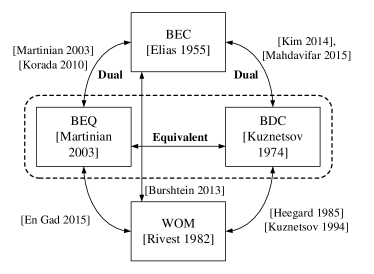
Figure 3: Relations between BEC, BDC, BEQ, and WOM.

Martinian and Yedidia [21] considered BEQ problems where the source vector consists of $\{0,1,*\}$ ($*$ denotes an erasure). Neither ones nor zeros may be changed, but erasures may be quantized to either zero or one. The erasures do not affect the distortion regardless of the value they are assigned since erasures represents source samples which are missing, irrelevant, or corrupted by noise. The BEQ problem with erasure probability $\alpha$ can be formulated as follows.

$$P(S=s)=\begin{cases}\alpha,&\text{if }s=*;\\ \frac{1-\alpha}{2},&\text{if }s=0~{}\text{or}~{}1\end{cases}$$ (33)

and the Hamming distortion $d_{H}(\cdot,\cdot)$ is given by

$$d_{H}(0,*)=d_{H}(1,*)=0,\quad d_{H}(0,1)=1.$$ (34)

The rate-distortion bound with zero distortion is given by

$$R_{\text{BEQ}}=1-\alpha.$$ (35)

In [21] the duality between the BEC and the BEQ was observed, and the authors showed that low-density generator matrix (LDGM) codes (i.e., the duals of LDPC codes) can achieve the $R_{\text{BEQ}}$ by modified message-passing algorithm. The computational complexity is $\mathcal{O}(nd_{\mathcal{G}})$ where $d_{\mathcal{G}}$ denotes the maximum degree of the bipartite graph $\mathcal{G}$ of the low-density generator matrix. In [31], it was shown that polar codes with an successive cancellation encoder can achieve $R_{\text{BEQ}}$ with $\mathcal{O}(n\log n)$.

From (33)–(35), we can claim that the BEQ with erasure probability $\alpha$ is equivalent to the BDC with defect probability $\beta$ if $\beta=1-\alpha$. We can observe that $s=*$ of the BEQ corresponds to $s=\lambda$ of the BDC, which represents normal cells by comparing (16) and (33). Also, $s=0$ and $s=1$ of the BEQ can be regarded as stuck-at 0 defects and stuck-at 1 defects, respectively. In addition, $R_{\text{BEQ}}=C_{\text{BEC}}=1-C_{\text{BDC}}$.

Since the BEQ is equivalent to the BDC, we can claim that RM codes achieve $R_{\text{BEQ}}$ due to Corollary 10. Hence, LDGM codes (duals of LDPC codes), polar codes, and RM codes achieve $R_{\text{BEQ}}$.

Inversely, the coding scheme for the BEQ can be applied to the BDC. Thus, $C_{\text{BDC}}$ can be achieved by LDGM codes and polar codes whose complexities are $\mathcal{O}(nd_{\mathcal{G}})$ and $\mathcal{O}(n\log n)$ respectively. It is important because the best known encoding complexity of capacity achieving scheme for the BDC was $\mathcal{O}(n\log^{2}n)$ in [17]. Also, note that the encoding complexity of coding schemes in [19] is $\mathcal{O}(n^{3})$.

The model of WOM was proposed for data storage devices where once a one is written on a memory cell, this cell becomes permanently associated with a one. Hence, the ability to rewrite information in these memory cells is constrained by the existence of previously written ones [22, 32]. Recently, the WOM model has received renewed attention as a possible channel model for flash memories due to their asymmetry between write and erase operations [33, 34].

In [32], it was noted that WOM are related to the BDC since the cells storing ones can be considered as stuck-at 1 defects. Moreover, Kuznetsov and Han Vinck [35] showed that additive encoding for the BDC can be used to achieve the capacity of WOM. Burshtein and Strugatski [36] proposed a capacity-achieving coding scheme for WOM with $\mathcal{O}(n\log n)$ complexity, which is based on polar codes and successive cancellation encoding [31]. Recently, En Gad et al. [37] related the WOM to the BEQ. Hence, LDGM codes and message-passing algorithm in [21] can be used for WOM. Note that the encoding complexity is $\mathcal{O}(nd_{\mathcal{G}})$.

Fig. 3 illustrates the relations between BEC, BDC, BEQ, and WOM. We emphasize that a coding scheme for one model can be applied to other models based on these relations. It is worth mentioning that RM codes, LDPC (or LDGM) codes, and polar codes can achieve the capacities of all these models. Their computational complexities are $\mathcal{O}(n^{3})$, $\mathcal{O}(nd_{\mathcal{G}})$, and $\mathcal{O}(n\log n)$, respectively.

III Locally Rewritable Codes (LWC)

Inspired by the duality between erasures and defects, we proposed locally rewritable codes (LWC). LWC were introduced to improve endurance and power consumption of resistive memories which can be modeled by the BDC. After briefly reviewing resistive memories and LRC, we explain LWC and their properties. The details of LWC can be found in [23].

III-A Resistive Memories

Resistive memory technologies are promising since they are expected to offer higher density than dynamic random-access memories (DRAM) and better speed performance than NAND flash memories [38]. Phase change memories (PCM) and resistive random-access memories (RRAM) are two major types of resistive memories. Both have attracted significant research interest due to their scalability, compactness, and simplicity.

The main challenges that prevent their large-scale deployment are endurance limit and power consumption [39, 40]. The endurance limit refers to the maximum number of writes before the memory becomes unreliable. Beyond the given endurance limit, resistive memory cells are likely to become defects [41, 42]. In addition, the power consumption depends on the number of writes. Hence, the number of writes is the key parameter for reliability of memory cells and power efficiency.

III-B Locally Repairable Codes (LRC)

An $(n,k,d,r)$ LRC is a code of length $n$ with information (message) length $k$, minimum distance $d$, and repair locality $r$. If a symbol in the LRC-coded data is lost due to a node failure, its value can be repaired (i.e. reconstructed) by accessing at most $r$ other symbols [25, 43].

One way to ensure fast repair is to use low repair locality such that $r\ll k$ at the cost of minimum distance $d$. The relation between $d$ and $r$ is given by [25]

$$d\leq n-k-\left\lceil\frac{k}{r}\right\rceil+2.$$ (36)

It is worth mentioning that this bound is a generalization of the Singleton bound. The LRC achieving this bound with equality are called optimal. Constructions of the optimal LRC were proposed in [44, 43, 45].

III-C Locally Rewritable Codes

As a toy example, suppose that $n$-cell binary memory has a single stuck-at defect. It is easy to see that this stuck-at defect can be handled by the following simple technique [6].

$$\mathbf{c}=(\mathbf{m},0)+\mathbf{1}_{n}\cdot p$$ (37)

where $G_{0}=\mathbf{1}_{n}$.

Suppose that $i$-th cell is a defect whose stuck-at value is $s_{i}\in\mathbb{F}_{2}$. If $i\in[n-1]$ and $s_{i}=m_{i}$, or if $i=n$ and $s_{n}=0$, then $p$ should be 0. Otherwise, $p=1$.

If there is no stuck-at defect among $n$ cells, then we can store $\mathbf{m}$ by writing $\mathbf{c}=(\mathbf{m},0)$ (i.e., $p=0$). Now, consider the case when stored information needs to be updated causing $\mathbf{m}$ to become $\mathbf{m}^{\prime}$. Usually, $\|\mathbf{m}-\mathbf{m}^{\prime}\|\ll n$, which happens often due to the updates of files. Instead of storing $\mathbf{m}^{\prime}$ into another group of $n$ cells, it is more efficient to store $\mathbf{m}^{\prime}$ by rewriting only $\|\mathbf{m}-\mathbf{m}^{\prime}\|$ cells. For example, suppose that $m_{i}^{\prime}\neq m_{i}$ for an $i\in[k]$ and $m_{j}^{\prime}=m_{j}$ for all other $j\in[k]\setminus i$. Then, we can store $k$-bit $\mathbf{m}^{\prime}$ by rewriting only one cell.

An interesting problem arises when a cell to be rewritten is defective. Suppose that $i$-th cell is a stuck-at defect whose stuck-at value is $s_{i}$. If $s_{i}=m_{i}\neq m_{i}^{\prime}$, then we should write $\mathbf{c}=(\mathbf{m},0)$ for storing $\mathbf{m}$. However, in order to store the updated information $\mathbf{m}^{\prime}$, we should write $\mathbf{c}^{\prime}=\overline{\mathbf{c}}=(\overline{\mathbf{m}},1)$ where $p=1$. Thus, $n-1$ cells should be rewritten to update one bit data $m_{i}^{\prime}$ without stuck-at error. The same thing happens when $s_{i}=m_{i}^{\prime}\neq m_{i}$. When considering endurance limit and power consumption, rewriting $n-1$ cells is a high price to pay for preventing one bit stuck-at error.

In order to relieve this burden, we can change (37) by introducing an additional parity bit as follows.

$$\mathbf{c} =\left(\mathbf{m}_{[1:\frac{n}{2}]},0,\mathbf{m}_{[\frac{n}{2}+1:n]},0\right)+G_{0}\mathbf{p}$$ (38)

$$=\left(\mathbf{m}_{[1:\frac{n}{2}]},0,\mathbf{m}_{[\frac{n}{2}+1:n]},0\right)+\begin{bmatrix}\mathbf{1}_{\frac{n}{2}}&\mathbf{0}_{\frac{n}{2}}\\ \mathbf{0}_{\frac{n}{2}}&\mathbf{1}_{\frac{n}{2}}\end{bmatrix}(p_{1},p_{2})$$ (39)

where $k=n-2$. For simplicity’s sake, we assume that $n$ is even. Then, $\mathbf{1}_{\frac{n}{2}}$ and $\mathbf{0}_{\frac{n}{2}}$ are all-ones and all-zeros column vectors with ${n}/{2}$ elements. By introducing an additional parity bit, we can reduce the number of rewriting cells from $n-1$ to $\frac{n}{2}-1$.

This idea is similar to the concept of Pyramid codes which are the early LRC [24]. For $n$ disk nodes, single parity check codes can repair one node failure (i.e., single erasure) by

$$\mathbf{1}_{n}^{T}\widehat{\mathbf{c}}=0$$ (40)

where $\widehat{\mathbf{c}}$ represents the recovered codeword from disk node failures. Assuming that $c_{i}$ is erased due to a node failure, $c_{i}$ can be recovered by

$$\widehat{c}_{i}=c_{i}=\sum_{j\in[n]\setminus i}{c_{j}}.$$ (41)

For this recovery, we should access $k=n-1$ nodes which degrades the repair speed. For more efficient repair process, we can add a new parity as follows.

$$H^{T}\widehat{\mathbf{c}}=\begin{bmatrix}\mathbf{1}_{\frac{n}{2}}&\mathbf{0}_{\frac{n}{2}}\\ \mathbf{0}_{\frac{n}{2}}&\mathbf{1}_{\frac{n}{2}}\end{bmatrix}^{T}\widehat{\mathbf{c}}=\mathbf{0}$$ (42)

Then, a failed node $c_{i}$ can be repaired by accessing only $\frac{n}{2}-1$ nodes. Note that the repair locality of (42) is $\frac{n}{2}-1$ whereas the repair locality of (40) is $n-1$ which is a simple but effecitve idea of Pyramid codes.

An interesting observation is that $G_{0}$ of (38) is the same as $H$ of (42). In addition, note that the number of resistive memory cells to be rewritten is the same as the number of nodes to be accessed in distributed storage systems. These observations can be connected to the duality between erasures and defects in Section II.

We define initial writing cost and rewriting cost which are related to write endurance and power consumption.

Definition 11 (Initial Writing Cost)

Suppose that $\mathbf{m}$ was stored by its codeword $\mathbf{c}$ in the initial stage of $n$ cells where all the normal cells are set to zeros. The writing cost is given by

$$\Delta(\mathbf{m})=\|\mathbf{c}\|-u_{\setminus 0}$$ (43)

where $u_{\setminus 0}$ denotes the number of stuck-at defects whose stuck-at values are nonzero.

In (43), we assume that there are $u$ defects among $n$ cells and $\mathbf{c}$ masks these $u$ stuck-at defects successfully. So, we do not need to write stuck-at defects since their stuck-at values are the same as corresponding elements of $\mathbf{c}$.

Definition 12 (Rewriting Cost)

Suppose that $\mathbf{m}$ was stored by its codeword $\mathbf{c}$ in $n$ cells. If $\mathbf{c}^{\prime}$ is rewritten to these $n$ cells to store the updated $\mathbf{m}^{\prime}$, the rewriting cost is given by

$$\Delta(\mathbf{m},\mathbf{m}^{\prime})=\|\mathbf{c}-\mathbf{c}^{\prime}\|$$ (44)

where we assume that both $\mathbf{c}$ and $\mathbf{c}^{\prime}$ mask stuck-at defects.

High rewriting cost implies that the states of lots of cells should be changed, which is harmful to endurance and power efficiency.

Now, we introduce the rewriting locality which affects initial writing cost and rewriting cost. The rewriting locality is a counterpart of repair locality of LRC. As repair locality is meaningful for a single disk failure, rewriting locality is valid when there is a single stuck-at defect among $n$ cells. In distributed storage systems, the most common case is a single node failure among $n$ nodes [24]. Similarly, for a proper defect probability $\beta$, we can claim that the most common scenario of resistive memories is that there is a single defect among $n$ cells.

Definition 13 (Information Rewriting Locality)

Suppose that $m_{i}$ for $i\in[k]$, i.e., information (message) part, should be updated to $m_{i}^{\prime}\neq m_{i}$ and the corresponding $i$-th cell is a stuck-at defect. If $m_{i}$ can be updated to $m_{i}^{\prime}$ by rewriting $r^{\star}$ other cells, then the $i$-th coordinate has information rewriting locality $r^{\star}$.

Lemma 14

[23] If the $i$-th coordinate for $i\in[k]$ has information rewriting locality $r^{\star}$, then there exists $\mathbf{c}_{0}\in\mathcal{C}_{0}$ such that $i\in\text{supp}(\mathbf{c}_{0})$ and $\left\|\mathbf{c}_{0}\right\|=r^{\star}+1$.

If a stuck-at defect’s coordinate is $i\in[k+1:n]$, i.e. parity location, then $\mathbf{m}$ can be updated to $\mathbf{m}^{\prime}$ by rewriting $\|\mathbf{m}-\mathbf{m}^{\prime}\|$ cells because of $\mathbf{c}_{0}=\mathbf{c}_{0}^{\prime}$. Thus, a stuck-at defect in the parity location is not related to rewriting. However, a stuck-at defect in the parity location affects initial writing. We will define parity rewriting locality as follows.

Definition 15 (Parity Rewriting Locality)

Suppose that only one nonzero symbol $m_{i}$ should be stored to the initial stage of $n$ cells. Note that there is a stuck-at defect in the parity location $j$ for $j\in[k+1:n]$ (i.e., parity part) and $s_{j}\neq 0$. If $m_{i}$ can be stored by writing at most $r^{\star}+1$ cells, then the $j$-th coordinate has parity rewriting locality $r^{\star}$.

Lemma 16

[23] If the $j$-th coordinate for $j\in[k+1:n]$ has parity rewriting locality $r^{\star}$, then there exists $\mathbf{c}_{0}\in\mathcal{C}_{0}$ such that $j\in\text{supp}(\mathbf{c}_{0})$ and $\left\|\mathbf{c}_{0}\right\|=r^{\star}+1$.

Definition 17 (Locally Rewritable Codes)

If any $i$-th coordinate for $i\in[n]$ has (information or parity) rewriting locality at most $r^{\star}$, then this code is called locally rewritable code (LWC) with rewriting locality $r^{\star}$. $(n,k,d^{\star},r^{\star})$ LWC code is a code of length $n$ with information length $k$, minimum distance $d^{\star}$, and rewriting locality $r^{\star}$.

Now, we show in the following theorem that rewriting locality $r^{\star}$ is an important parameter for rewriting cost.

Theorem 18

Suppose that $\mathbf{m}$ is updated to $\mathbf{m}^{\prime}$ by LWC with rewriting locality $r^{\star}$. If there is a single stuck-at defect in $n$ cells, then the rewriting cost $\Delta(\mathbf{m},\mathbf{m}^{\prime})$ is given by

$$\Delta(\mathbf{m},\mathbf{m}^{\prime})\leq\|\mathbf{m}-\mathbf{m}^{\prime}\|+r^{\star}-1.$$ (45)

Corollary 19

[23] If $\mathbf{m}$ is stored in the initial stage of $n$ cells with a single stuck-at defect, then the writing cost $\Delta(\mathbf{m})$ is given by

$$\Delta(\mathbf{m})\leq\|\mathbf{m}\|+r^{\star}.$$ (46)

Theorem 18 and Corollary 19 show that a small rewriting locality $r^{*}$ can reduce writing cost and rewriting cost, which is helpful for improving endurance and power consumption.

III-D Duality of LRC and LWC

In this subsection, we investigate the duality of LRC and LWC, which comes from the duality between erasures and defects in Section II. We show that existing construction methods of LRC can be used to construct LWC based on this duality. First, the relation between minimum distance $d^{\star}$ and rewriting locality $r^{\star}$ is observed.

Definition 20

If $\mathcal{C}_{0}$ is cyclic, then the LWC is called cyclic.

Lemma 21

[23] Let $\mathcal{C}_{0}$ denote a cyclic code whose minimum distance is $d_{0}$. Then, corresponding cyclic LWC’s rewriting locality is $r^{\star}=d_{0}-1$.

From the definition of $d^{\star}$ in (27), $d^{\star}=d_{0}^{\perp}$ which is the minimum distance of $\mathcal{C}_{0}^{\perp}$, namely, dual code of $\mathcal{C}_{0}$. Thus, the parameters of cyclic LWC is given by

$$(d^{\star},r^{\star})=(d_{0}^{\perp},d_{0}-1).$$ (47)

In [46, 47], an equivalent relation for cyclic LRC was given by

$$(d,r)=(d,d^{\perp}-1).$$ (48)

By comparing (47) and (48), we observed the duality between LRC and LWC. This duality is important since it indicates that we can construct LWC using existing construction methods of LRC as shown in the following theorem.

Theorem 22

[23] Suppose that $H_{\text{LRC}}\in\mathbb{F}_{q}^{n\times(n-k)}$ is the parity check matrix of cyclic LRC $\mathcal{C}_{\text{LRC}}$ with $(d,r)=(d,d^{\perp}-1)$. By setting $G_{0}=H_{\text{LRC}}$, we can construct cyclic LWC $\mathcal{C}_{\text{LWC}}$ with

$$(d^{\star},r^{\star})=(d,d^{\perp}-1).$$ (49)

In Theorem 9, we showed that the decoding failure probability of the optimal decoding scheme for the BEC is the same as the encoding failure probability of the optimal encoding scheme for the BDC. By setting $H=G_{0}$, capacity-achieving codes for the BDC can be constructed from state of art codes for the BEC. Similarly, Theorem 22 shows that we can construct $(n,k,d^{\star}=d,r^{\star}=d^{\perp}-1)$ LWC by using existing construction methods of $(n,k,d,r=d^{\perp}-1)$ LRC.

Remark 23 (Optimal Cyclic LWC)

[23] Theorem 22 shows that the optimal cyclic $(n,k,r,d)$ LRC can be used to construct the optimal cylic $(n,k,r^{\star},d^{\star})$ LWC such that

$$d^{\star}=n-k-\left\lceil\frac{k}{r^{\star}}\right\rceil+2.$$ (50)

Hence, the optimal LWC can be constructed from the optimal LRC.

Remark 24 (Bound of LWC)

[23] From Theorem 22 and Remark 23, we can claim the following bound for LWC.

$$d^{\star}\leq n-k-\left\lceil\frac{k}{r^{\star}}\right\rceil+2$$ (51)

which is equivalent to the bound for LRC given by (36).

TABLE II: Duality of LRC and LWC

	$(n,k,d,r)$ LRC	$(n,k,d^{\star},r^{\star})$ LWC
Application	Distributed storage systems	Resistive memories
	(system level)	(physical level)
Channel	Erasure channel	Defect channel
Encoding	$\mathbf{c}=G_{\text{LRC}}\mathbf{m}$	$\mathbf{c}=(\mathbf{m},\mathbf{0})+H_{\text{LRC}}\mathbf{p}$
Decoding	$H_{\text{LRC}}^{T}\widehat{\mathbf{c}}=\mathbf{0}$	$G_{\text{LRC}}^{T}\mathbf{c}=\widehat{\mathbf{m}}$
Bound	$d\leq n-k-\left\lceil\frac{k}{r}\right\rceil+2$	$d^{\star}\leq n-k-\left\lceil\frac{k}{r^{\star}}\right\rceil+2$
Trade-off	$d$ (reliability) vs.	$d^{\star}$ (reliability) vs.
	$r$ (repair efficiency)	$r^{*}$ (rewriting cost)

In Table II, the duality properties of LRC and LWC are summarized, which comes from the duality of the BEC and the BDC.

IV Conclusion

The duality between the BEC and the BDC was investigated. We showed that RM codes and duals of BCH codes achieve the capacity of the BDC based on this duality. This duality can be extended to the relations between BEC, BDC, BEQ, and WOM.

Based on these relations, we showed that RM codes achieve the capacity of the BDC with $\mathcal{O}(n^{3})$ and LDGM codes (duals of LDPC codes) achieve the capacity with $\mathcal{O}(nd_{\mathcal{G}})$. Also, polar codes can achieve the capacity with $\mathcal{O}(n\log n)$ complexity, which beats the best known result of $\mathcal{O}(n\log^{2}n)$.

Also, we proposed the LWC for resistive memories based on this duality, which are the counterparts of LRC for distributed storage systems. The proposed LWC can improve endurance limit and power consumption which are major challenges for resistive memories.

References

- [1] P. Elias, “Coding for two noisy channels,” in Proc. 3rd London Symp. Inf. Theory, London, U.K., 1955, pp. 61–76.
- [2] T. M. Cover and J. A. Thomas, Elements of Information Theory, 2nd ed. Hoboken, NJ: Wiley-Interscience, 2006.
- [3] M. G. Luby, M. Mitzenmacher, M. A. Shokrollahi, and D. A. Spielman, “Efficient erasure correcting codes,” IEEE Trans. Inf. Theory, vol. 47, no. 2, pp. 569–584, Feb. 2001.
- [4] A. Shokrollahi, “Raptor codes,” IEEE Trans. Inf. Theory, vol. 52, no. 6, pp. 2551–2567, Jun. 2006.
- [5] E. Arikan, “Channel polarization: A method for constructing capacity-achieving codes for symmetric binary-input memoryless channels,” IEEE Trans. Inf. Theory, vol. 55, no. 7, pp. 3051–3073, Jul. 2009.
- [6] A. V. Kuznetsov and B. S. Tsybakov, “Coding in a memory with defective cells,” Probl. Peredachi Inf., vol. 10, no. 2, pp. 52–60, Apr.–Jun. 1974.
- [7] L. A. Lastras-Montano, A. Jagmohan, and M. M. Franceschini, “Algorithms for memories with stuck cells,” in Proc. IEEE Int. Symp. Inf. Theory (ISIT), Austin, TX, USA, Jun. 2010, pp. 968–972.
- [8] A. Jagmohan, L. A. Lastras-Montano, M. M. Franceschini, M. Sharma, and R. Cheek, “Coding for multilevel heterogeneous memories,” in Proc. IEEE Int. Conf. Commun. (ICC), Cape Town, South Africa, May 2010, pp. 1–6.
- [9] E. Hwang, B. Narayanaswamy, R. Negi, and B. V. K. Vijaya Kumar, “Iterative cross-entropy encoding for memory systems with stuck-at errors,” in Proc. IEEE Global Commun. Conf. (GLOBECOM), Houston, TX, USA, Dec. 2011, pp. 1–5.
- [10] A. N. Jacobvitz, R. Calderbank, and D. J. Sorin, “Coset coding to extend the lifetime of memory,” in Proc. 19th IEEE Int. Symp. on High Performance Comput. Architecture (HPCA), Shenzhen, China, Feb. 2013, pp. 222–233.
- [11] Y. Kim and B. V. K. Vijaya Kumar, “Coding for memory with stuck-at defects,” in Proc. IEEE Int. Conf. Commun. (ICC), Budapest, Hungary, Jun. 2013, pp. 4347–4352.
- [12] ——, “Writing on dirty flash memory,” in Proc. 52nd Annu. Allerton Conf. Commun., Control, Comput., Monticello, IL, USA, Oct. 2014, pp. 513–520.
- [13] Y. Kim, R. Mateescu, S.-H. Song, Z. Bandic, and B. V. K. Vijaya Kumar, “Coding scheme for 3D vertical flash memory,” in Proc. IEEE Int. Conf. Commun. (ICC), London, UK, Jun. 2015, pp. 1861–1867.
- [14] C. Heegard and A. El Gamal, “On the capacity of computer memory with defects,” IEEE Trans. Inf. Theory, vol. 29, no. 5, pp. 731–739, Sep. 1983.
- [15] A. El Gamal and Y.-H. Kim, Network Information Theory. Cambridge, U.K.: Cambridge University Press, 2011.
- [16] B. S. Tsybakov, “Additive group codes for defect correction,” Probl. Peredachi Inf., vol. 11, no. 1, pp. 111–113, Jan.–Mar. 1975.
- [17] I. I. Dumer, “Asymptotically optimal linear codes correcting defects of linearly increasing multiplicity.” Probl. Peredachi Inf., vol. 26, no. 2, pp. 93–104, Apr.–Jun. 1990.
- [18] Y. Kim and B. V. K. Vijaya Kumar, “On the duality of erasures and defects,” arXiv preprint arXiv:1403.1897, vol. abs/1403.1897, 2014. [Online]. Available: http://arxiv.org/abs/1403.1897
- [19] H. Mahdavifar and A. Vardy, “Explicit Capacity Achieving Codes for Defective Memories,” in Proc. IEEE Int. Symp. Inf. Theory (ISIT), Jun. 2015, pp. 641–645.
- [20] S. Kudekar, S. Kumar, M. Mondelli, H. D. Pfister, E. Şaşoğlu, and R. Urbanke, “Reed-Muller codes achieve capacity on erasure channels,” arXiv preprint arXiv:1601.04689, Jan. 2016. [Online]. Available: http://arxiv.org/abs/1601.04689
- [21] E. Martinian and J. S. Yedidia, “Iterative quantization using codes on graphs,” in Proc. 41st Annu. Allerton Conf. Commun., Control, Comput., Monticello, IL, USA, 2003, pp. 1–10.
- [22] R. L. Rivest and A. Shamir, “How to reuse a write-once memory,” Information and control, vol. 55, no. 1, pp. 1–19, 1982.
- [23] Y. Kim, A. A. Sharma, R. Mateescu, S.-H. Song, Z. Z. Bandic, J. A. Bain, and B. V. K. Vijaya Kumar, “Locally rewritable codes for resistive memories,” in Proc. IEEE Int. Conf. Commun. (ICC), 2016, accepted.
- [24] C. Huang, M. Chen, and J. Li, “Pyramid codes: Flexible schemes to trade space for access efficiency in reliable data storage systems,” in Proc. IEEE Int. Symp. Netw. Comput. Appl. (NCA), Jul. 2007, pp. 79–86.
- [25] P. Gopalan, C. Huang, H. Simitci, and S. Yekhanin, “On the locality of codeword symbols,” IEEE Trans. Inf. Theory, vol. 58, no. 11, pp. 6925–6934, Nov. 2012.
- [26] T. Richardson and R. Urbanke, Modern coding theory. New York, NY, USA: Cambridge University Press, 2008.
- [27] C. Heegard, “Partitioned linear block codes for computer memory with “stuck-at” defects,” IEEE Trans. Inf. Theory, vol. 29, no. 6, pp. 831–842, Nov. 1983.
- [28] A. D. Wyner, “Recent results in the Shannon theory,” IEEE Trans. Inf. Theory, vol. 20, no. 1, pp. 2–10, Jan. 1974.
- [29] R. Zamir, S. Shamai, and U. Erez, “Nested linear/lattice codes for structured multiterminal binning,” IEEE Trans. Inf. Theory, vol. 48, no. 6, pp. 1250–1276, Jun. 2002.
- [30] F. J. MacWilliams and N. J. A. Sloane, The Theory of Error-Correcting Codes. Amsterdam, The Netherlands: North-Holland, 1977, pp. 282–283.
- [31] S. B. Korada and R. L. Urbanke, “Polar codes are optimal for lossy source coding,” IEEE Trans. Inf. Theory, vol. 56, no. 4, pp. 1751–1768, Apr. 2010.
- [32] C. Heegard, “On the capacity of permanent memory,” IEEE Trans. Inf. Theory, vol. 31, no. 1, pp. 34–42, Jan. 1985.
- [33] A. Jiang, “On the generalization of error-correcting WOM codes,” in Proc. IEEE Int. Symp. Inf. Theory (ISIT), Nice, France, Jun. 2007, pp. 1391–1395.
- [34] E. Yaakobi, S. Kayser, P. H. Siegel, A. Vardy, and J. K. Wolf, “Codes for write-once memories,” IEEE Trans. Inf. Theory, vol. 58, no. 9, pp. 5985–5999, Sep. 2012.
- [35] A. V. Kuznetsov and A. J. H. Vinck, “On the general defective channel with informed encoder and capacities of some constrained memories,” IEEE Trans. Inf. Theory, vol. 40, no. 6, pp. 1866–1871, Nov. 1994.
- [36] D. Burshtein and A. Strugatski, “Polar write once memory codes,” IEEE Trans. Inf. Theory, vol. 59, no. 8, pp. 5088–5101, 2013.
- [37] E. En Gad, W. Huang, Y. Li, and J. Bruck, “Rewriting flash memories by message passing,” in Proc. IEEE Int. Symp. Inf. Theory (ISIT), Hong Kong, Jun. 2015, pp. 646–650.
- [38] Intel and Micron, “3D XPoint Technology,” 2015. [Online]. Available: https://www.micron.com/about/innovations/3d-xpoint-technology
- [39] H.-S. P. Wong, S. Raoux, S. Kim, J. Liang, J. P. Reifenberg, B. Rajendran, M. Asheghi, and K. E. Goodson, “Phase change memory,” Proc. IEEE, vol. 98, no. 12, pp. 2201–2227, Dec. 2010.
- [40] H.-S. P. Wong, H.-Y. Lee, S. Yu, Y.-S. Chen, Y. Wu, P.-S. Chen, B. Lee, F. T. Chen, and M.-J. Tsai, “Metal–Oxide RRAM,” Proc. IEEE, vol. 100, no. 6, pp. 1951–1970, Jun. 2012.
- [41] S. Kim, P. Y. Du, J. Li, M. Breitwisch, Y. Zhu, S. Mittal, R. Cheek, T.-H. Hsu, M. H. Lee, A. Schrott, S. Raoux, H. Y. Cheng, S.-C. Lai, J. Y. Wu, T. Y. Wang, E. A. Joseph, E. K. Lai, A. Ray, H.-L. Lung, and C. Lam, “Optimization of programming current on endurance of phase change memory,” in Proc. Int. Symp. VLSI Technol., Syst., Appl. (VLSI-TSA), Apr. 2012, pp. 1–2.
- [42] A. A. Sharma, M. Noman, M. Abdelmoula, M. Skowronski, and J. A. Bain, “Electronic instabilities leading to electroformation of binary metal oxide-based resistive switches,” Adv. Functional Mater., vol. 24, no. 35, pp. 5522–5529, Jul. 2014.
- [43] I. Tamo and A. Barg, “A family of optimal locally recoverable codes,” IEEE Trans. Inf. Theory, vol. 60, no. 8, pp. 4661–4676, Aug. 2014.
- [44] N. Silberstein, A. S. Rawat, O. O. Koyluoglu, and S. Vishwanath, “Optimal locally repairable codes via rank-metric codes,” in Proc. IEEE Int. Symp. Inf. Theory (ISIT), Jul. 2013, pp. 1819–1823.
- [45] I. Tamo, D. S. Papailiopoulos, and A. G. Dimakis, “Optimal locally repairable codes and connections to matroid theory,” in Proc. IEEE Int. Symp. Inf. Theory (ISIT), Jul. 2013, pp. 1814–1818.
- [46] P. Huang, E. Yaakobi, H. Uchikawa, and P. H. Siegel, “Cyclic linear binary locally repairable codes,” in Proc. IEEE Inf. Theory Workshop (ITW), Apr. 2015, pp. 1–5.
- [47] I. Tamo and A. Barg, “Cyclic LRC codes and their subfield subcodes,” in Proc. IEEE Int. Symp. Inf. Theory (ISIT), Jul. 2015, pp. 1262–1266.