The variable spin-down rate of the transient magnetar XTE J1810–197

Abstract

We have analyzed XMM-Newton and Chandra observations of the transient magnetar XTE J1810–197  spanning more than 11 years, from the initial phases of the 2003 outburst to the current quiescent level. We investigated the evolution of the pulsar spin period and we found evidence for two distinct regimes: during the outburst decay, $\dot{\nu}$ was highly variable in the range $-(2-4.5)\times 10^{-13}$ Hz s^-1, while during quiescence the spin-down rate was more stable at an average value of $-1\times 10^{-13}$ Hz s^-1. Only during $\sim$3000 days (from MJD 54165 to MJD 56908) in the quiescent stage it was possible to find a phase-connected timing solution, with $\dot{\nu}=-4.9\times 10^{-14}$ Hz s^-1, and a positive second frequency derivative, $\ddot{\nu}=1.8\times 10^{-22}$ Hz s^-2. These results are in agreement with the behavior expected if the outburst of XTE J1810–197 was due to a strong magnetospheric twist.

1 Introduction

Magnetars are isolated neutron stars whose persistent emission and occasional outbursts are powered by magnetic energy (Duncan & Thompson 1992; Thompson & Duncan 1993; Paczynski 1992; see also Mereghetti 2008; Turolla et al. 2015). XTE J1810–197 was discovered with the Rossi X-ray Timing Explorer (RXTE) as a 5.45 s X-ray pulsar (Ibrahim et al., 2004) during a bright outburst in 2003, and associated to a previously known but unclassified ROSAT source. Further multiwavelength observations (Woods et al., 2005; Rea et al., 2004; Halpern et al., 2008), led to classify XTE J1810-197 as a magnetar candidate.

XTE J1810-197 is the prototype of transient members of this class of sources. It likely spent at least 23 years in quiescence (at a flux of $\sim$$7\times 10^{-13}$ erg s^-1 cm^-2, in the 0.5–10 keV energy band) before entering in outburst, in the 2003, when the flux increased by a factor of $\sim$100 (Gotthelf et al., 2004). For an estimated distance of $3.5$ kpc (Camilo et al., 2006; Minter et al., 2008), the maximum observed luminosity was $\sim$$10^{35}$ erg s^-1, but XTE J1810–197 might have reached an even higher luminosity, since the initial part of the outburst was missed. XTE J1810–197 was also the first magnetar from which pulsed radio emission was detected (Camilo et al., 2006, 2007). A large, unsteady spin-down of $\dot{P}\sim 10^{-11}$ s s^-1 was measured during the outburst decay through radio and X-ray observations, which suggested that the surface dipolar magnetic field is $\sim 2\times 10^{14}$ G (Gotthelf et al., 2004; Ibrahim et al., 2004; Camilo et al., 2006).

The spectrum of XTE J1810–197 during the outburst has been modeled by several authors with two or three blackbody components of different temperature. The colder one has been interpreted as the (persistent) emission from the whole neutron star surface, while the hotter ones have been associated to cooling regions responsible for the outburst (Gotthelf et al., 2004; Bernardini et al., 2009, 2011; Alford & Halpern, 2016). The appearance of hot spots could be due to the release of (magnetic) energy deep in the crust, or to Ohmic dissipation of back-flowing currents as they hit the star surface (Perna & Gotthelf, 2008; Albano et al., 2010; Beloborodov, 2009; Pons & Rea, 2012). The X-ray pulse profile was energy-dependent and time-variable in amplitude, and it could be generally modelled by a single sinusoidal function (e.g. Ibrahim et al., 2004; Camilo et al., 2007; Bernardini et al., 2009, 2011; Alford & Halpern, 2016).

Table 1: Log of the XMM-Newton and Chandra observations.

Obs.	Satellite	Obs. ID	Epocha	Duration
No.			MJD	ks
1	Chandra	4454	52878.9386632	4.3
2	XMM-Newton	0161360301	52890.5595740	9.5
3	XMM-Newton	0161360401	52890.7083079	2.1
4	XMM-Newton	0152833201	52924.1677914	7.0
5	Chandra	5240	52944.6289075	5.4
6	XMM-Newton	0161360501	53075.4952632	17.2
7	XMM-Newton	0164560601	53266.4995129	26.7
8	XMM-Newton	0301270501	53447.9973027	40.0
9	XMM-Newton	0301270401	53633.4453382	40.0
10	XMM-Newton	0301270301	53806.7899360	41.8
11	Chandra	6660	53988.8111877	31.8
12	XMM-Newton	0406800601	54002.0627203	48.1
13	XMM-Newton	0406800701	54165.7713547	60.2
14	XMM-Newton	0504650201	54359.0627456	72.7
15	Chandra	7594	54543.0034395	31.5
16	XMM-Newton	0552800301	54895.5656089	4.3
17	XMM-Newton	0552800201	54895.6543341	63.6
18	XMM-Newton	0605990201	55079.6256771	19.4
19	XMM-Newton	0605990301	55081.5548494	17.7
20	XMM-Newton	0605990401	55097.7062563	12.0
21	Chandra	11102	55136.6570779	26.5
22	Chandra	12105	55242.6870526	15.1
23	Chandra	11103	55244.7426533	14.6
24	XMM-Newton	0605990501	55295.1863453	7.7
25	Chandra	12221	55354.1368700	11.5
26	XMM-Newton	0605990601	55444.6796630	9.1
27	Chandra	13149	55494.1643981	16.8
28	Chandra	13217	55600.9885520	16.2
29	XMM-Newton	0671060101	55654.0878884	17.4
30	XMM-Newton	0671060201	55813.3872852	13.7
31	Chandra	13746	55976.3735837	22.5
32	Chandra	13747	56071.3650797	22.1
33	XMM-Newton	0691070301	56176.9826811	15.7
34	XMM-Newton	0691070401	56354.1968379	15.7
35	XMM-Newton	0720780201	56540.8584298	21.2
36	Chandra	15870	56717.3097928	22.1
37	XMM-Newton	0720780301	56720.9705351	22.7
38	Chandra	15871	56907.9508362	21.7

^a Mean time of the observation.

Here we report on the pulse period evolution of XTE J1810–197 exploiting the full set of XMM-Newton and Chandra X-ray observations carried out in the years 2003–2014 during the outburst decay and in the following quiescent period.

2 Observations and data reduction

We made use of 24 XMM-Newton and 14 Chandra observations of XTE J1810–197  totalizing an exposure time of $\sim$$830$ ks (see the log of observations in Table 1).

The XMM-Newton data were reduced using SAS v. 14.0.0 and the most recent calibrations. We used the data obtained with the EPIC instrument, which consists of one pn camera and two MOS cameras. For each observation, we selected events with single and double pixel events (pattern$\leq$4) for EPIC-pn and single, double, triple and quadruple pixel events for EPIC-MOS (pattern$\leq$12). We set ‘flag=0’ so to exclude bad pixels and events coming from the CCD edge. The source and background events were extracted from 30^′′ and 60^′′ radius circular regions, respectively. Time intervals with high particle background were removed.

In three observations (7, 13 and 35) we found inconsistent values between the phases of the pulses derived (as described in the next Section) from the MOS and pn data. This is due to a known sporadic problem in the timing of EPIC-pn data, causing a shift of $\pm$1 second in the times attributed to the counts. We identified the times at which the problems occurred and corrected the data by adding (or subtracting) 1 second to the photon time of arrival from the instant when the problem occurred (see Martin-Carrillo et al., 2012).

The Chandra observations were reduced using the ciao v.4.7 software and adopting the standard procedures. Source events were extracted from a region of 20^′′ radius around the position of XTE J1810–197  and background counts from a similar region close to the source.

Photon arrival times of both satellites were converted to the Solar system barycenter using the milliarcsec radio position of XTE J1810–197 (RA = 272.462875 deg, Dec. = –19.731092 deg, (J2000); Helfand et al. 2007) and the JPL planetary ephemerides DE405.

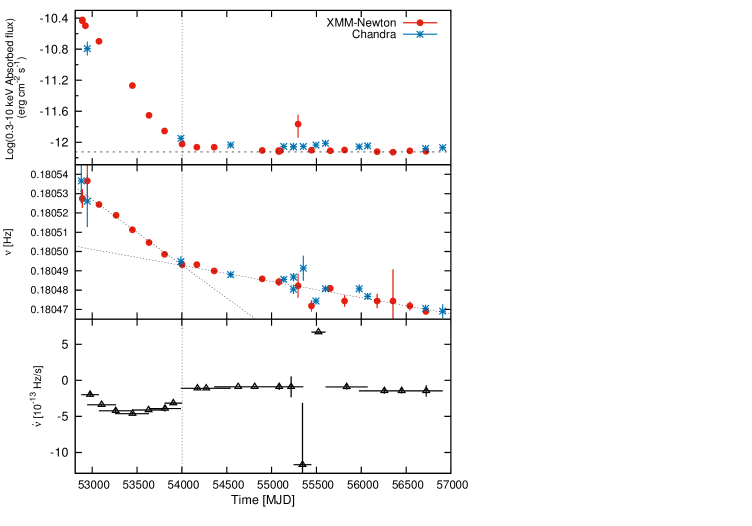
Figure 1: Top panel: evolution of the logarithmic absorbed flux in the 0.3-10 keV energy range. The dashed line is the linear fit to the data after MJD 54500. The errors are at $90\%$ confidence level. Center panel: spin frequency along the outburst of XTE J1810–197 as found in the single observations. The dashed lines indicate the fits with two linear functions to the data before and after MJD 54000. Bottom panels: frequency derivatives as measured by linear fits of small sub-set of observations. The horizontal error bars indicate the time interval spanned by the observations used in each fit.
The vertical, dashed line indicates the epoch after which is possible to phase-connect the data. Errors in the center and bottom panels are at $1\sigma$.

3 Timing analysis

In order to study the evolution of the spin frequency from outburst to quiescence (i.e. covering the whole data set) we initially measured the spin frequency in each individual pointing by applying a phase-fitting technique in every observation. The phase of a pulse is defined as $\phi=\phi_{0}+\int\nu dt$, where $\nu$ is the spin frequency. If the coherence of the signal is maintained between subsequent observations, the data can be be fitted by the polynomial:

$$\phi(t)=\phi_{0}+\nu_{0}(t-T_{0})+\cfrac{1}{2}\dot{\nu}(t-T_{0})^{2}+\cfrac{1}{6}\ddot{\nu}(t-T_{0})^{3}+...$$ (1)

where $T_{0}$ is the reference epoch, $\nu_{0}$ is the frequency at $T_{0}$, $\dot{\nu}$ is the spin frequency derivative and $\ddot{\nu}$ is second-order spin frequency derivative (e.g. Dall’Osso et al., 2003, for more details).

Thanks to the large counting statistics of each single observation, it was possible to obtain accurate measurements of the frequencies by applying the phase-fitting technique to a number of short time intervals (durations from 300 s to 5 ks, depending on the counting statistics) within each observation and we were able to align the pulse-phases by use only the linear term of Eq. 1. The frequencies derived in this way are plotted as a function of time in the middle panel of Figure 1, while in the top panel we show the flux evolution of XTE J1810–197.

To derive the fluxes plotted in Figure 1, we fitted the time-averaged spectra of each observation with a model consisting of two to three blackbodies (see e.g. Bernardini et al. 2009; Alford & Halpern 2016 for more details). The interstellar absorption was kept fixed to the value of $5.7\times 10^{21}$ cm^-2, derived from the spectrum of the first XMM-Newton observation. The temperatures that we found for the three blackbodies ($\sim$0.1, 0.3 and 0.5 keV) are consistent with those reported in Bernardini et al. (2009) and Alford & Halpern (2016), to which we refer for more details. The maximum flux observed by XMM-Newton during the outburst was $(3.18\pm 0.04)\times 10^{-11}$ erg cm^-2 s^-1 (absorbed flux in the 0.3-10 keV energy range). The flux decreased until about MJD 54500, after which it remained rather constant (see also Gotthelf & Halpern 2007; Bernardini et al. 2011; Alford & Halpern 2016). We found that the flux slowly decreased, finally reaching a constant value of $(7.5\pm 0.2)\times 10^{-13}$ erg cm^-2 s^-1, which we derived by fitting with a constant the fluxes of all the observations after MJD 54500 (see Fig. 1-top panel). This value is within the range of fluxes measured by ROSAT, ASCA and Einstein before the onset of the outburst ($(5-10)\times 10^{-13}$ erg cm^-2 s^-1; Gotthelf et al. 2004).

It is clear from Fig. 1 that the source timing properties tracked remarkably well the evolution of the flux. The average spin-down rate was larger during the first 3-4 years, during the outburst decay, and then it decreased while the source was in (or close to) quiescence. We can distinguish two time intervals, separated at MJD $\sim 54000$, in which a linear fit can approximately describe the frequency evolution. The slopes of the two linear functions are $(-3.9\pm 0.2)\times 10^{-13}$ Hz s^-1 ($\chi^{2}_{\nu}/dof=6.7/9$) and $(-1.00\pm 0.05)\times 10^{-13}$ Hz s^-1 ($\chi^{2}_{\nu}/dof=1.8/24$) before and after MJD 54000, respectively. These values represent the long-term averaged spin-down rates, but the residuals of the linear fits indicate that the time evolution of the frequency derivative is more complex. To better investigate this behavior, we performed several linear fits to small groups of consecutive frequency measurements. We adopted a moving-window approach by using partially overlapping sets of points. In this way we obtained the $\dot{\nu}$ values plotted in the bottom panel of Figure 1. They show a highly variable spin-down rate, especially during the outburst decay, when it ranged from $-4.5\times 10^{-13}$ Hz s^-1 to $-0.5\times 10^{-13}$ Hz s^-1.

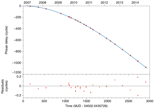
Figure 2: Phase-connection of $\sim 3000$ days of XMM-Newton and Chandra data (observations from 13 to 38) using a third order polynomial function. Top: the red points are the measured phases, one for each observation, and the solid line is the best fit model; bottom: residuals with respect to the best fit model.

Phase-coherent timing solutions for XTE J1810–197 have been reported for the initial part of the outburst (Ibrahim et al., 2004; Camilo et al., 2007). We tried to phase-connect all the XMM-Newton and Chandra observations, but this turned out to be rather difficult due to the large timing noise. However, we were able to find a phase-connected solution for the data during quiescence (i.e. all the observations obtained after MJD 54100), as follows. For each observation, we folded the EPIC (pn plus MOS) or Chandra data at a frequency of 0.18048 Hz (corresponding to $P=5.54078$ s, the average spin period after MJD 54100). For each observation the phase of the pulsation was then derived by fitting a constant plus a sinusoid to the folded pulse profile in the 0.3-10 keV energy range. We initially aligned, with only the linear term in Eq. 1, the XMM-Newton observations 18 and 19 that were the most closely spaced ($\sim$2 days). Then, we included one by one the other observations, as the uncertainty on the best-fit parameters became increasingly smaller allowing us to connect more distant points. We included higher order derivatives only if the improvement in the fit was significant in the timing solution. After the inclusion of Chandra observations 21 and 22, the quadratic term became statistically significant, while the third order polynomial term was needed after the inclusion of observations 25 and 26. The best fit parameters of the final solution are reported in Table 2 and the fit is shown in Figure 4. The fit with $\nu$, $\dot{\nu}$ and $\ddot{\nu}$ has $\chi_{\nu}^{2}$= 65.7 (for 20 dof). Such a large value reflects the presence of a strong timing noise. In fact, the residuals shown in the lower panel of Figure 4 indicate significant deviations from the best fit solution, especially during the last 1000 days, when they are as large as $\sim$0.2 cycles in phase.

Some timing irregularity occurred also when the source was in quiescence. In particular, around MJD $\sim$55400 the spin-down rate was much larger than the quiescent average value and larger than that seen during the outburst decay. Quite remarkably, also a spin-up episode was detected (see Figure 1-bottom). This is better illustrated in Figure 3 which shows the frequency measurements around this time. Unfortunately, the sparse coverage and the large error bars of some points do not allow us to establish whether this was a sudden event, like an anti-glitch, or simply due to an increased timing noise episode. Assuming that the time irregularity is an anti-glitch, we fitted the data in the time range MJD 54300–57000, with the following simple model:

$\nu(t)=\nu_{0}+\dot{\nu_{0}}\cdot t$                                      for $t<t_{g}$

$\nu(t)=\nu_{0}+\dot{\nu_{0}}\cdot t+\Delta\nu\cdot e^{(-(t-t_{g})/\tau)}$     for $t>t_{g}$

where $\tau$ is the decay time and $t_{g}$ is the time of the glitch, which we kept fixed in the fit. If the glitch occurred immediately after observation 25 ($t_{g}=55354$), we obtained a good fit ($\chi^{2}_{\nu}=1.14$ for 21 dof, shown by the solid line in Figure 3) with $\Delta\nu=(6.5\pm 5.8)\times 10^{-5}$ Hz, $\tau=51\pm 21$ days, $\nu_{0}=0.18093(3)$ Hz and $\dot{\nu_{0}}=-9.4(3)\times 10^{-14}$ Hz s^-1. If instead the glitch occurred at observation 26 ($t_{g}=55444$), we obtain $\Delta\nu<1\times 10^{-4}$ Hz and $\tau<200$ days ($3\sigma$ upper limits).

4 Discussion

Variations in the spin-down rate are not uncommon in magnetars and have been observed both in transient and persistent sources. They are believed to originate from changes in the magnetosphere geometry and particles outflow which produce a varying torque on the neutron star. Since also the emission properties from magnetars depend on the evolution of their dynamic magnetospheres, some correlation between spin-period evolution and radiative properties is not surprising.

Table 2: Best-fit timing solution of the XMM-Newton and Chandra observations. Errors are at 1$\sigma$.

Parameter		Units
Time range	54165–56908	MJD
T0a	54002.0430729	MJD
$\nu_{0}$	0.1804821(1)	Hz
$\dot{\nu}$	$-4.9(2)\times 10^{-14}$	Hz s-1
$\ddot{\nu}$	$1.8(1)\times 10^{-22}$	Hz s-2
$P$	5.540716(3)	s
$\dot{P}$	$1.51(7)\times 10^{-12}$	s s-1
$\ddot{P}$	$-5.5(4)\times 10^{-21}$	s s-2
$\chi_{\nu}^{2}(dof)$	65.7 (20)

^a Reference epoch.

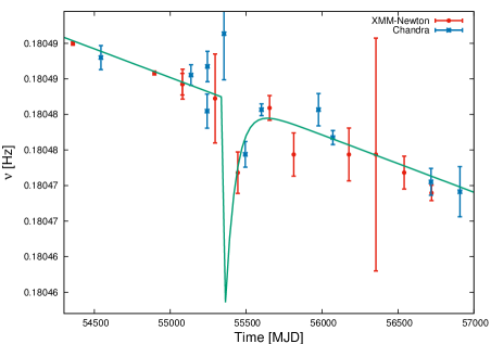
Figure 3: Frequencies measured around the time of the possible anti-glitch. The solid line is the best-fit discussed in the text.

The most striking examples, among persistent magnetars, are given by SGR 1806–20 and 1E 1048.1–5937. The average spin-down rate of SGR 1806–20, as well as its spectral hardness, increased in the $\sim 4$ years of enhanced bursting activity which led to the giant flare of December 2004 (Mereghetti et al., 2005). However, a further increase (by a factor of 2–3) of the long term spin-down rate occurred both in 2006 and 2008, while the flux and bursting rate showed no remarkable changes (Younes et al., 2015). In 1E 1048.1–5937, significant enhancements of the spin-down rate, which then subsided through repeated oscillations, have been observed to lag the occurrence of X-ray outbursts (Archibald et al., 2015). Other persistent magnetars, for which phase-coherent timing solutions extending over several years could be mantained, showed $\dot{\nu}$ variations and/or glitches, sometimes (but not always) related to changes in the source flux and the emission of bursts (e.g. Dib & Kaspi, 2014).

Transient magnetars offer, in principle, the best opportunity to investigate the correlations between the variations in the spin-down rate and the radiative properties. However, the observations of transient magnetars carried out up to now have shown a variety of different behaviors. Furthermore, for many of them, no detailed information is available on the spin-down during the quiescent state, that instead in this work we now have found for XTE J1810–197 . No firm conclusion on the evolution of the spin-down rate could be derived from the two outbursts of CXOU J164710.2–455216, for which a positive $\ddot{\nu}$ was reported only during the decay of the first outburst, while the insufficient time coverage prevented such a measure for the second one (Rodríguez Castillo et al., 2014). A positive $\ddot{\nu}$ was reported for both Swift J1822.3–1606 (which went in outburst in July 2011 and was subsequently monitored for about 500 days; Rodríguez Castillo et al. 2015), as well as for SGR J1935+2154 (outburst in July 2014, time coverage $\sim 260$ days; Israel et al. 2016), and, tentatively, also for SGR 0501+4516 (for this source observations actually covered part of the quiescent state but phase connection along the entire dataset could not be ensured; Camero et al. 2014). On the other hand, an increase of the spin-down rate during the outburst decay was reported for SGR J1745–29 (Kaspi et al., 2014; Coti Zelati et al., 2015).

Our analysis of XMM-Newton and Chandra data spanning 11 years has shown that in the transient magnetar XTE J1810–197 the spin frequency evolution tracked remarkably well the luminosity state. During the outburst decay, the average spin-down rate was $(-3.9\pm 0.2)\times 10^{-13}$ Hz s^-1, but large variations around this value were seen, as already noticed by several authors (Halpern & Gotthelf, 2005; Camilo et al., 2007; Bernardini et al., 2009). During the long quiescent state after the end of the outburst, the average spin-down rate was a factor of $\sim 4$ smaller. Although some timing noise was still present, the variations in $\dot{\nu}$ were smaller in the quiescent state, except for a few months in Summer 2010. The timing irregularities in that period might have been caused by the occurrence of an anti-glitch, similar to that seen in the persistent magnetar 1E 2259+586 (Archibald et al., 2013). We found that the pulse-shape in the 0.3–10 keV energy range was nearly sinusoidal and the pulse fraction decreased during the outburst decay, as already reported by e.g. Perna & Gotthelf (2008), Albano et al. (2010) and Bernardini et al. (2009). We note that the pulse-shape remained nearly sinusoidal also during quiescence (see also Bernardini et al. 2011; Alford & Halpern 2016).

The spectral properties of magnetars are commonly explained in terms of the twisted magnetosphere model (Thompson et al., 2002), according to which part of the magnetic helicity is transferred from the internal to the external magnetic field, which acquires a non-vanishing toroidal component (a twist). The currents required to support the twisted external field resonantly up-scatter thermal photons emitted by the star surface, leading to the formation of the power-law tails observed up to hundreds of keV. Since twisted fields have a weaker dependence on the radial distance with respect to a dipole, the higher magnetic field at the light cylinder radius results in an enhanced spin-down rate. The increased activity of magnetars is often associated to the development (or an increase) of a twist, which should lead to higher fluxes, local surface temperature increases, harder spectra and larger spin-down rates. However, this holds for globally twisted fields (meaning that the twist affects the entire external field). The transport of helicity from the interior is mediated by the star crust: in order to occur the crust must yield, allowing a displacement of the field lines. Crustal displacements are small compared to the star radius, so the twist is most likely localized to a bundle of field lines anchored on the displaced platelet (Beloborodov, 2009). Once implanted, the twist must necessarily decay to maintain its own supporting currents, unless energy is constantly supplied from the star interior. The sudden appearance of a localized twist and its subsequent decay can explain some of the observed properties of transient magnetars (Beloborodov, 2009; Albano et al., 2010), including the fact that transient spectra are often thermal, as in the case of XTE J1810–197, since resonant Compton scattering may be not very effective, although the mechanism responsible for the heating of the star surface is still unclear (either Ohmic dissipation by backflowing currents or deep crustal heating; Beloborodov 2009; Pons & Rea 2012). If strong enough, a localized twist can still influence the spin-down rate, which is expected to increase first and then decrease as the magnetosphere untwists, as we observed in XTE J1810–197.

5 Conclusions

XTE J1810–197 was the first transient magnetar to be discovered and it is probably one of the best studied. In particular, it has been possible to trace in great detail its spectral properties over the long ($\sim 3$ years) outburst decay and to monitor it during quiescence for several years afterwards. By investigating the evolution of its spin frequency with all the available XMM-Newton and Chandra data, we found evidence for two distinct regimes: during the outburst decay, $\dot{\nu}$ was highly variable in the range $-(2-4.5)\times 10^{-13}$ Hz s^-1, while during quiescence the spin-down rate was more stable and had an average value smaller by a factor $\sim 4$.

This evolution of the spin-down rate is in agreement with the suggestion that the outburst of transient magnetars may be caused by a strong twist of a localized bundle of magnetic field lines (Beloborodov, 2009). Evidences for an evolution of $\dot{\nu}$ in other transient magnetars are far less conclusive, possibly reflecting the fact that, if the twist is not very strong, or the twisted bundle too localized, its effect on the spin-down rate are smaller. A detailed calculation of the spin-down torque for a spatially-limited twisted field requires a full non-linear approach and has not been presented yet. Beloborodov (2009) discussed a simple estimate, valid for small twists ($\psi<1\ \mathrm{rad}$)

$$\Delta\mu/\mu\sim(\psi^{2}/4\pi)\log(u_{*}/u_{\mathrm{LC}})\,,$$ (2)

where $\Delta\mu$ is the “equivalent” increase in the dipole moment produced by the twist and $u$ is the area of the j-bundle, evaluated at the star surface and at the light cylinder. Since $\Delta\dot{\nu}/\nu\sim 2\Delta\mu/\mu$, a fractional variation of $\dot{\nu}$ of a factor of $\sim 4$, as observed (see Figure 1, lower panel), can not be achieved with a small twist, $\psi<1$. This indicates that the (maximal) twist in XTE J1810–197 was most probably larger, $\psi\ga 1\ \mathrm{rad}$, so that equation (2) does not hold anymore. A quite large value of the twist in the outburst of XTE J1810–197 was also inferred by Beloborodov (2009), on the (qualitative) basis that only a strong twist can produce a change of the spin-down rate.

ERRATUM: “The variable spin-down rate of the transient magnetar XTE J1810–197”

Prompted by the recent paper by Camilo et al. (2016), we re-examined our phase-connected timing solution for XTE J1810–197 (Pintore et al. 2016), and we found a flaw in the procedure to compute the errors during some steps of our analysis. Due to this mistake, the phase-connected solution on 3000 days of X-ray data (reported in Tab. 2 and Fig. 2 of Pintore et al. 2016) is wrong.

With the new analysis of the data, we can phase-connect 13 observations with a good fit ($\chi^{2}_{\nu}$ (dof)$=0.9(9)$; solution 1 in Tab.3 and Fig.4-top), from MJD 55079 to MJD 55814 (observations from 18 to 30 of Pintore et al. 2016). The inclusion of also the two observations at MJD 55976 and MJD 56071 (observations 31 and 32) yields best fit parameters (solution 2 in Tab.3 and Fig.4-bottom) consistent with those obtained by Camilo et al. (2016) for the same set of observations, but with a higher $\chi_{\nu}^{2}$ with respect to solution 1.

The table and figures reported here supersede Tab. 2 and Fig. 2 of Pintore et al. (2016). We note that these changes do not affect the main conclusions of that paper.

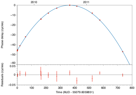
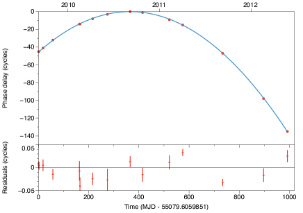
Figure 4: Phase-connection of $\sim 800$ (left) and $\sim 1000$ (right) days of XMM-Newton and Chandra data using a third order polynomial function. Top panels: the red points are the measured phases, one for each observation, and the solid line is the best fit model; bottom panels: residuals with respect to the best-fit model.

Table 3: Best-fitting timing solutions for 13 (solution 1) and 15 (solution 2) XMM-Newton and Chandra observations. Errors are at 1$\sigma$.

Parameter	Solution 1	Solution 2
Time range (MJD)	55079–55814	55079–56071 MJD TDB
T0a (MJD TDB)	55444.0	55444.0
$\nu_{0}$ (Hz)	0.18048121335(44)	0.18048121599(27)
$\dot{\nu}$ (Hz s-1)	$-9.2059(16)\times 10^{-14}$	$-9.2085(16)\times 10^{-14}$
$\ddot{\nu}$ (Hz s-2)	$5.7(3)\times 10^{-23}$	$3.80(13)\times 10^{-23}$
$P$ (s)	5.540742892(14)	5.540742811(8)
$\dot{P}$ (s s-1)	$2.8262(5)\times 10^{-12}$	$2.8270(5)\times 10^{-12}$
$\ddot{P}$ (s s-2)	$-1.75(9)\times 10^{-21}$	$-1.16(4)\times 10^{-21}$
$\chi_{\nu}^{2}$ (dof)	0.9 (9)	5.0 (11)

^a Reference epoch.

References

Camilo F., Ransom S. M., Halpern J. P., Alford J. A. J., Cognard I., Reynolds J. E., Johnston S., Sarkissian J., van Straten W., 2016, ApJ, 820, 110

Pintore F., Bernardini F., Mereghetti S., Esposito P., Turolla R., Rea N., Coti Zelati F., Israel G. L., Tiengo A., Zane S., 2016, MNRAS, 458, 2088

References

- Albano et al. (2010) Albano A., Turolla R., Israel G. L., Zane S., Nobili L., Stella L., 2010, ApJ, 722, 788
- Alford & Halpern (2016) Alford J., Halpern J., 2016, ArXiv e-prints
- Archibald et al. (2013) Archibald R. F., Kaspi V. M., Ng C.-Y., Gourgouliatos K. N., Tsang D., Scholz P., Beardmore A. P., Gehrels N., Kennea J. A., 2013, Nature, 497, 591
- Archibald et al. (2015) Archibald R. F., Kaspi V. M., Ng C.-Y., Scholz P., Beardmore A. P., Gehrels N., Kennea J. A., 2015, ApJ, 800, 33
- Beloborodov (2009) Beloborodov A. M., 2009, ApJ, 703, 1044
- Bernardini et al. (2009) Bernardini F., Israel G. L., Dall’Osso S., Stella L., Rea N., Zane S., Turolla R., Perna R., Falanga M., Campana S., Götz D., Mereghetti S., Tiengo A., 2009, A&A, 498, 195
- Bernardini et al. (2011) Bernardini F., Perna R., Gotthelf E. V., Israel G. L., Rea N., Stella L., 2011, MNRAS, 418, 638
- Camero et al. (2014) Camero A., Papitto A., Rea N., Viganò D., Pons J. A., Tiengo A., Mereghetti S., Turolla R., Esposito P., Zane S., Israel G. L., Götz D., 2014, MNRAS, 438, 3291
- Camilo et al. (2007) Camilo F., Ransom S. M., Halpern J. P., Reynolds J., 2007, ApJ, 666, L93
- Camilo et al. (2006) Camilo F., Ransom S. M., Halpern J. P., Reynolds J., Helfand D. J., Zimmerman N., Sarkissian J., 2006, Nature, 442, 892
- Coti Zelati et al. (2015) Coti Zelati F., Rea N., Papitto A., Viganó D., Pons J. A., Turolla R., Esposito P., Haggard D., Baganoff F. K., Ponti G., et al. I., 2015, MNRAS, 449, 2685
- Dall’Osso et al. (2003) Dall’Osso S., Israel G. L., Stella L., Possenti A., Perozzi E., 2003, ApJ, 599, 485
- Dib & Kaspi (2014) Dib R., Kaspi V. M., 2014, ApJ, 784, 37
- Duncan & Thompson (1992) Duncan R. C., Thompson C., 1992, ApJ, 392, L9
- Gotthelf & Halpern (2007) Gotthelf E. V., Halpern J. P., 2007, Ap&SS, 308, 79
- Gotthelf et al. (2004) Gotthelf E. V., Halpern J. P., Buxton M., Bailyn C., 2004, ApJ, 605, 368
- Halpern & Gotthelf (2005) Halpern J. P., Gotthelf E. V., 2005, ApJ, 618, 874
- Halpern et al. (2008) Halpern J. P., Gotthelf E. V., Reynolds J., Ransom S. M., Camilo F., 2008, ApJ, 676, 1178
- Helfand et al. (2007) Helfand D. J., Chatterjee S., Brisken W. F., Camilo F., Reynolds J., van Kerkwijk M. H., Halpern J. P., Ransom S. M., 2007, ApJ, 662, 1198
- Ibrahim et al. (2004) Ibrahim A. I., Markwardt C. B., Swank J. H., Ransom S., Roberts M., Kaspi V., Woods P. M., Safi-Harb S., Balman S., Parke W. C., Kouveliotou C., Hurley K., Cline T., 2004, ApJ, 609, L21
- Israel et al. (2016) Israel G. L., Esposito P., Rea N., Coti Zelati F., Tiengo A., Campana S., Rodriguez Castillo S. M. G. A., Gotz D., Burgay M., Possenti A., Zane S., Turolla R., 2016, ArXiv e-prints
- Kaspi et al. (2014) Kaspi V. M., Archibald R. F., Bhalerao V., Dufour F., Gotthelf E. V., An H., Bachetti M., Beloborodov A. M., Boggs S. E., et al. C., 2014, ApJ, 786, 84
- Martin-Carrillo et al. (2012) Martin-Carrillo A., Kirsch M. G. F., Caballero I., Freyberg M. J., Ibarra A., Kendziorra E., Lammers et al. 2012, A&A, 545, A126
- Mereghetti (2008) Mereghetti S., 2008, A&A Rev., 15, 225
- Mereghetti et al. (2005) Mereghetti S., Götz D., von Kienlin A., Rau A., Lichti G., Weidenspointner G., Jean P., 2005, ApJ, 624, L105
- Minter et al. (2008) Minter A. H., Camilo F., Ransom S. M., Halpern J. P., Zimmerman N., 2008, ApJ, 676, 1189
- Paczynski (1992) Paczynski B., 1992, Acta Astronomica, 42, 145
- Perna & Gotthelf (2008) Perna R., Gotthelf E. V., 2008, ApJ, 681, 522
- Pons & Rea (2012) Pons J. A., Rea N., 2012, ApJ, in press (astro-ph/1203.4506)
- Rea et al. (2004) Rea N., Testa V., Israel G. L., Mereghetti S., Perna R., Stella L., Tiengo A., Mangano V., Oosterbroek T., Mignani R., Lo Curto G., Campana S., Covino S., 2004, A&A, 425, L5
- Rodríguez Castillo et al. (2014) Rodríguez Castillo G. A., Israel G. L., Esposito P., Pons J. A., Rea N., Turolla R., Viganò D., Zane S., 2014, MNRAS, 441, 1305
- Rodríguez Castillo et al. (2015) Rodríguez Castillo G. A., Israel G. L., Tiengo A., Salvetti D., Turolla R., Zane S., Rea N., Esposito P., Mereghetti S., Perna R., Stella L., Pons J. A., Campana S., Götz D., Motta S., 2015, ArXiv e-prints
- Thompson & Duncan (1993) Thompson C., Duncan R. C., 1993, ApJ, 408, 194
- Thompson et al. (2002) Thompson C., Lyutikov M., Kulkarni S. R., 2002, ApJ, 574, 332
- Turolla et al. (2015) Turolla R., Zane S., Watts A. L., 2015, Reports on Progress in Physics, 78, 116901
- Woods et al. (2005) Woods P. M., et al., 2005, ApJ, 629, 985
- Younes et al. (2015) Younes G., Kouveliotou C., Kaspi V. M., 2015, ApJ, 809, 165