Infinitely many monotone Lagrangian tori in del Pezzo surfaces

Abstract.

We construct almost toric fibrations (ATFs) on all del Pezzo surfaces, endowed with a monotone symplectic form. Except for $\mathbb{C}P^{2}\#\overline{\mathbb{C}P^{2}}$, $\mathbb{C}P^{2}\#2\overline{\mathbb{C}P^{2}}$, we are able to get almost toric base diagrams (ATBDs) of triangular shape and prove the existence of infinitely many symplectomorphism (in particular Hamiltonian isotopy) classes of monotone Lagrangian tori in $\mathbb{C}P^{2}\#k\overline{\mathbb{C}P^{2}}$ for $k=0,3,4,5,6,7,8$. We name these tori $\Theta^{n_{1},n_{2},n_{3}}_{p,q,r}$. Using the work of Karpov-Nogin, we are able to classify all ATBDs of triangular shape. We are able to prove that $\mathbb{C}P^{2}\#\overline{\mathbb{C}P^{2}}$ also have infinitely many monotone Lagrangian tori up to symplectomorphism and we conjecture that the same holds for $\mathbb{C}P^{2}\#2\overline{\mathbb{C}P^{2}}$. Finally, the Lagrangian tori $\Theta^{n_{1},n_{2},n_{3}}_{p,q,r}\subset X$ can be seen as monotone fibers of ATFs, such that, over its edge lies a fixed anticanonical symplectic torus $\Sigma$. We argue that $\Theta^{n_{1},n_{2},n_{3}}_{p,q,r}$ give rise to infinitely many exact Lagrangian tori in $X\setminus\Sigma$, even after attaching the positive end of a symplectization to $\partial(X\setminus\Sigma)$.

1. Introduction

We say that two Lagrangians submanifolds of a symplectic manifold $X$ belong to the same symplectomorphism class if there is a symplectomorphism of $X$ sending one Lagrangian to the other. Similar for Hamiltonian isotopy class.

In [Via2], it is explained how to get infinitely many symplectomorphism classes of monotone Lagrangian tori in $\mathbb{C}P^{2}$. The idea is to construct different almost toric fibrations (denoted from here by ATF) [Sym, LS] of $\mathbb{C}P^{2}$. The procedure starts by applying nodal trades [Sym, LS] to the corners of the moment polytope and subsequently applying a series of nodal slides [Sym, LS] through the monotone fiber of the ATF. In that way we obtain infinitely many monotone Lagrangian tori $T(a^{2},b^{2},c^{2})$ as the central fibre of some almost toric base diagram (denoted from here by ATBD) describing an ATF. They are indexed by Markov triples $(a,b,c)$, i.e., positive integer solutions of $a^{2}+b^{2}+c^{2}=3abc$. We refer the reader to [Via2] for a detailed account.

It is clear that the technique to construct ATFs and potentially get infinitely many symplectomorphism classes of monotone Lagrangian tori would also apply for any monotone toric symplectic 4-manifolds. In this paper we show that we can actually construct ATFs in all monotone del Pezzo surfaces,i.e. , $\mathbb{C}P^{1}\times\mathbb{C}P^{1}$ and $\mathbb{C}P^{2}\#k\overline{\mathbb{C}P^{2}}$, $0\leq k\leq 8$.

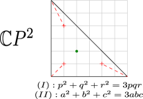
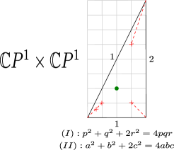
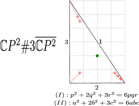
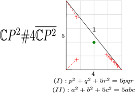
Figure 1. ATBDs of $\mathbb{C}P^{2}$, $\mathbb{C}P^{1}\times\mathbb{C}P^{1}$, $\mathbb{C}P^{2}\#2\overline{\mathbb{C}P^{2}}$, $\mathbb{C}P^{2}\#4\overline{\mathbb{C}P^{2}}$ of triangular shape. Near each base diagram is the corresponding Markov type I and II equations (Definition 2.12).

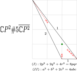
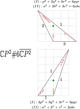
Figure 2. ATBDs of $\mathbb{C}P^{2}\#5\overline{\mathbb{C}P^{2}}$, $\mathbb{C}P^{2}\#6\overline{\mathbb{C}P^{2}}$ of triangular shape. Below each base diagram is the corresponding Markov type I and II equations.

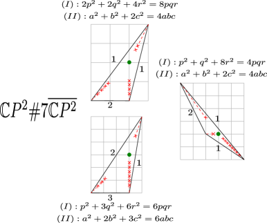
Figure 3. ATBDs of $\mathbb{C}P^{2}\#7\overline{\mathbb{C}P^{2}}$ of triangular shape. Close to each base diagram is the corresponding Markov type I and II equations.

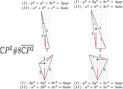
Figure 4. ATBDs of $\mathbb{C}P^{2}\#8\overline{\mathbb{C}P^{2}}$ of triangular shape. Close to each base diagram is the corresponding Markov type I and II equations.

In [OO1, OO2], Ohta-Ono proved that the diffeomorphism type of any closed monotone symplectic 4-manifold is $\mathbb{C}P^{1}\times\mathbb{C}P^{1}$ and $\mathbb{C}P^{2}\#k\overline{\mathbb{C}P^{2}}$, $0\leq k\leq 8$, based on the work of McDuff [McD1] and Taubes [Tau1, Tau2, Tau3]. Also, in [McD2], McDuff showed that uniqueness of blowups (of given sizes) for 4-manifolds of non-simple Seiberg-Witten type (which includes $\mathbb{C}P^{2}$). Finally, from the uniqueness of the monotone symplectic form for $\mathbb{C}P^{2}$ and $\mathbb{C}P^{1}\times\mathbb{C}P^{1}$ [Gro, McD1, Tau1, Tau3] (see also the excelent survey [Sal]), we get uniqueness of monotone symplectic structures on $\mathbb{C}P^{1}\times\mathbb{C}P^{1}$ and $\mathbb{C}P^{2}\#k\overline{\mathbb{C}P^{2}}$, $0\leq k\leq 8$. We refer the later as del Pezzo surfaces thinking of them endowed with a monotone symplectic form.

The algebraic count of Maslov index 2 pseudo-holomorphic disks with boundary in a monotone Lagrangian $L$ and relative homotopy class $\beta$ is an invariant of the symplectomorphism class of $L$, first pointed out in [EP] (we believe that the formal proof needs the work of [Laz]). To distinguish the monotone Lagrangian tori we built in $\mathbb{C}P^{2}$, we used an invariant among monotone Lagrangian $L$ in the same symplectomorphism class based on the above count [Via2]. We named it the boundary Maslov-2 convex hull $\mho_{L}$ [Via2, Section 4], which is the convex hull in $H_{1}(L)$ of the set formed by the boundary of Maslov index 2 classes in $\pi_{2}(X,L)$ that have non-zero enumerative geometry. In other words, it is the convex hull for the Newton polytope of the superpotential function - for definition of the superpotential we refer the reader to [Aur1, Aur2, FOOO1].

For computing the above invariant, we employed the neck-stretching technique [EGH, BEH⁺] to get a degenerated limit of pseudo-holomorphic disks with boundary in $T(a^{2},b^{2},c^{2})$ inside the weighted projective space $\mathbb{C}P(a^{2},b^{2},c^{2})$. We then used positivity of intersection for orbifold disks [CR, Che] in the weighted projective space $\mathbb{C}P(a^{2},b^{2},c^{2})$, together with the computation of holomorphic disks away from the orbifold points [CP] to be able to compute $\mho_{T(a^{2},b^{2},c^{2})}$, the boundary Maslov-2 convex hull for $T(a^{2},b^{2},c^{2})$. It follows that $\mho_{T(a^{2},b^{2},c^{2})}$ is incongruent (not related via $SL(2,\mathbb{Z})$ upon a choice of basis for the respectives 1st homotopy groups) to $\mho_{T(d^{2},e^{2},f^{2})}$, if $\{a,b,c\}\neq\{d,e,f\}$.

The aim of this paper is to prove:

Theorem 1.1.

There are infinitely many symplectomorphism classes of monotone Lagrangian tori inside:

1. $\mathbb{C}P^{1}\times\mathbb{C}P^{1}$ and $\mathbb{C}P^{2}\#k\overline{\mathbb{C}P^{2}}$, $k=0,3,4,5,6,7,8$;

2. $\mathbb{C}P^{2}\#\overline{\mathbb{C}P^{2}}$;

The proof of items (a), (b) of the above theorem differ a little.

To prove Theorem 1.1 (a) we show that for $\mathbb{C}P^{1}\times\mathbb{C}P^{1}$ and $\mathbb{C}P^{2}\#k\overline{\mathbb{C}P^{2}}$, $k=0,3,4,5,6,7,8$ we can build almost toric base diagrams of triangular shape described in Figures 1, 2, 3, 4.

We call a mutation in an ATBD with respect to a node $s$ if we apply a nodal slide operation [Sym, LS] (we always slide the node to pass through the monotone fiber) together with a transferring the cut operation [Via2], with respect to $s$.

The affine lengths of the edges of the ATBDs depicted in Figures 1-4 are related to solutions of Markov type II equations of the form

$$k_{1}a^{2}+k_{2}b^{2}+k_{3}c^{2}=Kk_{1}k_{2}k_{3}abc.\ \ \eqref{eq: Markovtype}$$

We can apply a mutation $(a,b,c)\to(a^{\prime}=Kk_{2}k_{3}bc-a,b,c)$ to obtain a new solution of the same Markov type II equation.

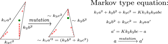
Figure 5. Mutation on ATBD of triangular shape corresponds to mutation on Markov type II triples.

Suppose we have an ATBD related to the Markov type II equation (2.2), for some $K,k_{1},k_{2},k_{3}$. We prove on Section 4 (Lemma 4.2) that a mutation on an ATBD with respect to all nodes in the same cut corresponds to a mutation on the respective Markov type II triple solution of (2.2), as ilustrated in Figure 5.

But the affine lengths do not determine the ATBDs of triangular shape, see Figure 3. What does is the node type (Definition 2.1). An ATBD of node-type $((n_{1},p),(n_{2},q),(n_{3},r))$, must have $(p,q,r)$ satisfying the Markov type I equation:

$$n_{1}p^{2}+n_{2}q^{2}+n_{3}r^{2}=\sqrt{dn_{1}n_{2}n_{3}}pqr,\ \ \eqref{eq: MarkovI}$$

We name $\Theta^{n_{1},n_{2},n_{3}}_{p,q,r}$ the monotone fiber inside an ATBD of node-type $((n_{1},p),(n_{2},q),(n_{3},r))$ (we are assuming that the fiber lives on the complement of all the cuts). We can aplly the same ideas of the proof of Theorem 1.1 of [Via2][Section 4] to compute $\mho_{\Theta^{n_{1},n_{2},n_{3}}_{p,q,r}}$, the boundary Maslov-2 convex hull for each $\Theta^{n_{1},n_{2},n_{3}}_{p,q,r}$.

Let’s call the limit orbifold (Definition 2.13) of an ATBD the orbifold described by the moment polytope given by deleting the cuts of the ATBD (here we assume that the cuts are all in the eigendirection of the monodromy around the respective node). Informally, we think that we nodal slide all the nodes of the ATBD towards the edge, so in the limit the described by the corresponding ATF is “degenerating” to the limit orbifold.

In the proof of Theorem 1.1 (a), we look at degenerated limit of pseudo-holomorphic disks with boundary in $T(k_{1}a^{2},k_{2}b^{2},k_{3}c^{2})$, which lives in the limit orbifold of the corresponding ATBD. One important aspect we use to compute $\mho_{\Theta^{n_{1},n_{2},n_{3}}_{p,q,r}}$ is positivity of intersection between the degenerated limit of pseudo-holomorphic curves in the limit orbifold and pre-image of the edges of the limit orbifold’s moment polytope. We may loose this property if the moment polytope of the limit orbifold is not a triangle.

For the cases $\mathbb{C}P^{2}\#k\overline{\mathbb{C}P^{2}}$, $k=1,2$, we can also construct infinitely many ATBDs, each one describing an ATF with a monotone Lagrangian torus fiber, for instance the ones in Figures 6,7. Let’s name $T_{1}(a,b)$ the monotone torus fiber of the ATF of $\mathbb{C}P^{2}\#\overline{\mathbb{C}P^{2}}$ depicted in Figure 6, similar $T_{2}(a,b)\subset\mathbb{C}P^{2}\#2\overline{\mathbb{C}P^{2}}$ depicted in Figure 7.

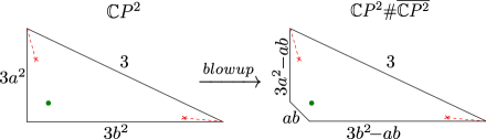
Figure 6. ATBD of $\mathbb{C}P^{2}\#\overline{\mathbb{C}P^{2}}$ as a blowup of an ATBD of $\mathbb{C}P^{2}$ with affine lengths proportional to the squares of a Markov triple of the form $(1,a,b)$, with $b>a$.

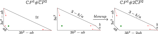
Figure 7. ATBD of $\mathbb{C}P^{2}\#2\overline{\mathbb{C}P^{2}}$ as a blowup of an ATBD of $\mathbb{C}P^{2}\#\overline{\mathbb{C}P^{2}}$.

Eventhough we expect that each of these monotone Lagrangian mutually belong to different symplectomorphism classes, for $k=1,2$, we can’t show that using our technique. That is because we loose the positivity of intersection property for the limit orbifold and hence we can’t describe the boundary Maslov-2 convex hull of $T_{1}(a,b)$ and $T_{2}(a,b)$.

Nonetheless, for $k=1$, we can extract enough information about the boundary Maslov-2 convex hull to show that there are infinitely many symplectomorphism classes of monotone Lagrangian tori. More precisely, we can show that $\mho_{T_{1}(a,b)}$ must contain a vertex with affine angle $b^{\prime}=3a-b$ (the norm of determinant of the matrix formed by the primitive vectors as columns). We can also show that $\mho_{T_{1}(a,b)}$ is compact. Since we have infinitely many possible values for $b^{\prime}$, we must have infinitely many boundary Maslov-2 convex hulls. Therefore, Theorem 1.1 (b) holds.

So we have:

Conjecture 1.2.

There are infinitely many symplectomorphism classes of monotone Lagrangian tori inside $\mathbb{C}P^{2}\#2\overline{\mathbb{C}P^{2}}$.

Consider two monotone Lagrangian fibres of ATFs for which their ATBDs are related via one mutation. The algebraic count of Maslov index 2 pseudo-holomorphic disks for this tori is expected to vary according to wall-crossing formulas [Aur1, Aur2, GU, Via1]. In view of that we conjecture:

Conjecture 1.3.

The boundary Maslov-2 convex hull of a monotone Lagrangian fiber of an ATF described by an ATBD (whose cuts are inside eigenline of the respective node) is determined by the limit orbifold. Actually, the vertices of the convex hull should be the primitive vectors that describe the fan of the limit orbifold.

Which would allow us to conclude:

Conjecture 1.4.

Suppose we have two monotone Lagrangian fibres of ATFs of the same symplectic manifold, described by ATBDs whose orbifold limits are different. Then they are not symplectomorphic.

So we expect to have many more symplectomorphism classes of monotone Lagrangian tori than the ones of $\Theta^{n_{1},n_{2},n_{3}}_{p,q,r}$.

Consider now a ATBD of triangular shape described in Figures 1-4. Call $X$ the corresponding del Pezzo surface. Since they have no rank $0$ singularity, there is a smooth symplectic torus $\Sigma$ living over the edge of the base of the corresponding ATF and representing the anti-canonical class [Sym]. We can assume that a neighbourhood of $\Sigma$ remains invariant under the mutations of the ATBD’s, so $\Sigma$ is always living over the edge of the base of corresponding ATF.

Hence all the tori $\Theta^{n_{1},n_{2},n_{3}}_{p,q,r}\subset X$ live on $X\setminus\Sigma$ and are in different Hamiltonian isotopic classes there. The complement of (a neighbourhood) of $\Sigma$ has a contactype boundary $V$ with a Liouville vector field pointing outiside. Hence we can atach the positive half of a symplectization, obtaining $(X\setminus\Sigma)\cup(V\times[0,+\infty))$. We can show

Theorem 1.5.

The tori $\Theta^{n_{1},n_{2},n_{3}}_{p,q,r}\subset(X\setminus\Sigma)\cup(V\times[0,+\infty))$ belong to mutually different Hamiltonian isotopy classes.

For the case of the complement of an elliptic curve in $\mathbb{C}P^{2}$ the above theorem can be proved by Tonkonog using a different approach. By looking at a Lagrangian skeleton of $X\setminus\Sigma$, Shende-Teumann-Williams [STW] can show that there exists infinitelly many distinct subcategories of the category of microlocal sheaves on the Lagrangian skeleton. The Lagrangian skeleton is given by attaching Lagrangian disks to an torus. The subcategories mentioned above corresponds to sheaves on the tori given by mutations that are equivalent to the ones we see in ATBDs, see Section 6.1.

The rest of the paper is organised as follows:

We start defining some terminology in Section 2. We suggest the reader to move directly to Section 3 and use Section 2 only if some terminology is not clear from the context.

In Section 3, we describe how to obtain all the ATBDs of Figures 1-4, also showing how to “create space” to perform a blowup by changing the ATF. In Section 3.5, we make a small digression to describe how to perform an almost toric blowup. We believe that the reader should become easily acquainted with the operations on the ATBDs and be able to deduce the moves just by looking at the Figures 9-12, 15,16. Nonetheless, we provide explicit description of each operation on the ATBDs.

In Section 4, we show that mutations of Markov type I and II equations corresponds to mutations of ATBDs of triangular shape. We also show that any monotone ATBD of triangular shape is node-related (Definition 2.12) to a Markov type I equation. It follows from [KN, Section 3.5] that Figures 1-4 provide a complete list of ATBDs of triangular shape for del Pezzo surfaces.

In Section 5, we compute the boundary Maslov-2 convex hull $\mho_{\Theta^{n_{1},n_{2},n_{3}}_{p,q,r}}$ (Theorem 5.1), which finishes the proof of Theorem 1.1(a). We prove Theorem 1.1(b) in Section 5.2 and Theorem 1.5 in Section 5.3

In Section 6 we relate our work with [STW], by pointing out that the complement of the symplectic torus $\Sigma$ in the anti-canonical class is obtained from attaching (Weinstein handles along the boundary of) Lagrangian discs to the (co-disk bundle of the) monotone fiber of each ATBD. In particular, these tori are exact on the complement of $\Sigma$. We also relate our work with [Kea2], where Keating shows how modality 1 Milnor fibers $\mathcal{T}_{p,q,r}$, for $(p,q,r)\in\{(3,3,3),(2,4,4),(2,3,6)\}$ compatify to del Pezzo surfaces of degree $d=3,2,1$. It follows from Theorem 1.5, that there are infinitely many Hamiltonian isotopic classes of exact tori in $\mathcal{T}_{p,q,r}$, for $(p,q,r)\in\{(3,3,3),(2,4,4),(2,3,6)\}$. Also, in [Kea1, Section 7.4], Keating mention that all Milnor fibers $\mathcal{T}_{p,q,r}$ are obtained by attaching Lagrangian discs to a Lagrangian torus as described in [STW]. We conjecture then that there are infinitely many exact tori in $\mathcal{T}_{p,q,r}$. We believe this conjecture is also made in [STW]. In Section 6.3, we point out that the Markov type I equations appear before related to $3$-blocks exceptional collections in the del Pezzo surfaces [KN] and $\mathbb{Q}$-Gorenstein smoothing of weighted projetive spaces to del Pezzo surfaces [HP]. We enquire if there is a correspondence between ATBDs - $3$-blocks exceptional collections - $\mathbb{Q}$-Gorenstein smoothings. Finally, we relate the ATBD of $\mathbb{C}P^{1}\times\mathbb{C}P^{1}$ in Figure 1 with the singular Lagrangian fibration given by Fukaya-Oh-Ohta-Ono in [FOOO3], as well as a similar ATBD of $\mathbb{C}P^{2}$ with the singular Lagrangian fibration described in [Wu]. In [FOOO3, FOOO2] it was shown that there are a continuous of non-displaceable fibers in the monotone $\mathbb{C}P^{1}\times\mathbb{C}P^{1}$ and in $\mathbb{C}P^{2}\#k\overline{\mathbb{C}P^{2}}$ for $k\geq 2$ with respect to some symplectic form, but not monotone for $k>2$. We ask what ATBDs have a continuous of non-displaceable fibers.

Acknowledgements

We would like to thanks Ivan Smith, Dmitry Tonkonog, Georgious Dimitroglou Rizell, Denis Auroux, Jonathan David Evans and Kaoru Ono for useful conversations. Section 6 was very much motivated by talks given by Vivek Shende and Ailsa Keating at the Symplectic Geometry and Topology Workshop held in Uppsala on September 2015.

2. Terminology

Before we describe how to get almost toric fibrations on all del Pezzo surfaces, let’s fix some terminology. A lot of the terminology can be intuitively grasped, so we suggest the reader to move on to the next section and only use this section as a reference for terminology.

We recall that a primitive vector on the standard lattice of $\mathbb{R}^{2}$ is an integer vector that is not a positive multiple of another integer vector.

We also recall that an ATBD is the image of an affine map from the base of an ATF, minus a set of cuts, to $\mathbb{R}^{2}$ endowed with the standar affine structure. Let $s$ be a node of an ATF and $R^{+}$ an eigenray leaving $s$. Suppose we have an ATBD where the cut associated to $s$ is a ray equals to “the image of” $R^{+}$.

Definition 2.1.

We say that $R^{+}$ is an $(m,n)$-eigenray of an ATBD if it points towards the node in the direction of the primitive vector $(m,n)\in\mathbb{Z}^{2}\subset\mathbb{R}^{2}$. We also say that $s$ is an $(m,n)$-node of the ATBD.

We recall from [Via2, Definition 2.1] that, a transferring the cut operation with respect to $R^{+}$ gives another ATBD, representing the same ATF, but with a cut (the image of) $R^{-}$, the eigenray other than $R^{+}$ pertaining to the same eigenline. In this paper we overlook the fact that we have two options (left and right) for performing a transferring the cut operation, since the two resulting ATBD are related via $SL(2,\mathbb{Z})$.

Definition 2.2.

We call a mutation with respect to a $(m,n)$-node an operation on an ATBD containing a monotone fibre consisting of: a nodal slide [Sym, Section 6.1] of the corresponding $(m,n)$-eigenray passing through the monotone fibre; and one transferring the cut operation with respect to the same eigenray.

Definition 2.3.

A total mutation is a mutation with respect to all $(m,n)$-nodes, for some $(m,n)$.

Definition 2.4.

A Markov type I equation, is an integer equation for a triple $(p,q,r)$ of the form:

$$n_{1}p^{2}+n_{2}q^{2}+n_{3}r^{2}=\sqrt{dn_{1}n_{2}n_{3}}pqr,$$ (2.1)

for some constants $d,n_{1},n_{2},n_{3}\in\mathbb{Z}_{>0}$, so that $dn_{i}n_{j}\equiv 0\mod n_{k}$, $\{i,j,k\}=\{1,2,3\}$ and $dn_{1}n_{2}n_{3}$ is a square. A solution $(p,q,r)$ is called a Markov type I triple, if $p,q,r\in\mathbb{Z}_{>0}$.

Definition 2.5.

Let $(p,q,r)$ be a Markov type I triple. The Markov type I triple
$(p^{\prime}=\sqrt{\frac{dn_{2}n_{3}}{n_{1}}}qr-p,q,r)$ is said to be obtained from $(p,q,r)$ via a mutation with respect to $p$. Analogous for mutation with respect to $q$ and $r$.

Definition 2.6.

A Markov type II equation, is an integer equation for a triple $(a,b,c)$ of the form:

$$k_{1}a^{2}+k_{2}b^{2}+k_{3}c^{2}=Kk_{1}k_{2}k_{3}abc,$$ (2.2)

for some constants $K,k_{1},k_{2},k_{3}\in\mathbb{Z}_{>0}$. A solution $(a,b,c)$ is called a Markov type II triple, if $a,b,c\in\mathbb{Z}_{>0}$.

Definition 2.7.

Let $(a,b,c)$ be a Markov type II triple. The Markov type II triple $(a^{\prime}=Kk_{2}k_{3}bc-a,b,c)$ is said to be obtained from $(a,b,c)$ via a mutation with respect to $a$. Analogous for mutation with respect to $b$ and $c$.

Definition 2.8.

A Markov type I/II triple $(p,q,r)$/$(a,b,c)$ is said to be minimum if it minimizes the sum $p+q+r$/$a+b+c$, among Markov type I/II triples.

Definition 2.9.

An ATBD of triangular shape is an ATBD whose cuts are all in the direction of the respective eigenrays of the associated node and whose closure is a triangle in $\mathbb{R}^{2}$.

Definition 2.10.

An ATBD of length type $(A,B,C)$, is an ATBD of triangular shape whose edges have affine lengths proportional to $(A,B,C)$.

Definition 2.11.

An ATBD of node type $((n_{1},p),(n_{2},q),(n_{3},r))$, is an ATBD of triangular shape with the three cuts $R_{1},R_{2},R_{3}$ contains respectively $n_{1},n_{2},n_{3}$ nodes, and the determinant of primitive vectors of the edges connecting at the cut $R_{1}$, respectively $R_{2}$, $R_{3}$, have norm equals to $n_{1}p^{2}$, respectively, $n_{2}q^{2}$, $n_{3}r^{2}$.

Note that the above definition can be generalized to any ATBD whose cuts are all in the direction of an eigenray leaving the respective node.

Definition 2.12.

We say that an ATBD is length-related to an Markov type II equation (2.2) if it is of length type $(k_{1}a^{2},k_{2}b^{2},k_{3}c^{2})$, for some Markov type II triple $(a,b,c)$.
We say that an ATBD is node-related to an Markov type I equation (2.1) if it is of node type
$((n_{1},p),(n_{2},q),(n_{3},r))$, for some Markov type I triple $(p,q,r)$, and moreover the total space of the corresponding ATF is a del Pezzo of degree $d$, i.e., for $\mathbb{C}P^{2}\#k\overline{\mathbb{C}P^{2}}$, $d=9-k$, and for $\mathbb{C}P^{1}\times\mathbb{C}P^{1}$, $d=2$.

We also define the limit orbifold of an ATBD:

Definition 2.13.

Given an ATBD, its limit orbifold is the orbifold for which the moment map image is equal to the ATBD without the nodes and cuts, which are replaced by corners (usually not smooth).

3. Almost toric fibrations of del Pezzo surfaces

To perform a blowup in the symplectic category [MS], one deletes a symplectic ball $B(\epsilon)$ of radius $\epsilon$ and collapses the fibres of the Hopf fibration of $\partial B(\epsilon)$ to points. In particular, the blowup depends on the radius $\epsilon$ one takes. In a toric symplectic manifold, one can perform a blowup near a rank $0$ singularity and remain toric, provided one chooses an small enough ball compatible with the toric fibration, see Figure 8.

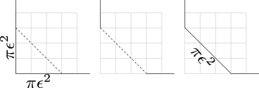
Figure 8. Blowup of a ball $B(\epsilon)$ centered at a rank 0 singularity in a toric manifold

We recall that a symplectic manifold $(X,\omega)$ is said to be monotone if there exists $C>0$ such that $\forall H\in\pi_{2}(X)$:

$$\int_{H}\omega=C\mathrm{c}_{1}(H).$$ (3.1)

And Lagrangian $L\subset X$ is said to be monotone if there exists $C_{L}>0$ such that $\forall\beta\in\pi_{2}(X,L)$:

$$\int_{\beta}\omega=C_{L}\mu_{L}(\beta),$$ (3.2)

where $\mu_{L}$ is the Maslov index.

Since $\mathrm{c}_{1}=2\mu_{L|\pi_{2}(X)}$, if $\pi_{2}(X)\neq 0$, then $2C=C_{L}$. Also, if $L$ is orientable $\mu_{L}(\beta)\in 2\mathbb{Z}$.

The monotonicity condition is then affected by the size of the symplectic blow up. In dimension 4, when we perform a symplectic blowup, we modify the second homology group by adding a spherical class - coming from the quotient of $S^{3}$ under the Hopf fibration - of Chern number 1. Therefore to keep monotonicity one must choose the radius of the symplectic ball, so that the quotient sphere has the appropriate symplectic area (3.1).

One is able to perform symplectic blowup in one, two or three corners of the moment polytope of $\mathbb{C}P^{2}$ to obtain monotone toric structures on $\mathbb{C}P^{2}\#\overline{\mathbb{C}P^{2}}$, $\mathbb{C}P^{2}\#2\overline{\mathbb{C}P^{2}}$, $\mathbb{C}P^{2}\#3\overline{\mathbb{C}P^{2}}$. But one cannot go further, since it is not possible to torically embed a ball of appropriate radius centered in a corner of the moment polytope of $\mathbb{C}P^{2}\#3\overline{\mathbb{C}P^{2}}$, depicted in the left-most picture of Figure 9.

Nonetheless, it is possible to create some space for the blowup if we only require to remain almost toric.

We are now ready to describe ATFs for all del Pezzo surfaces. In all ATBDs apearing on Figures 9, 10, 11, 12, 15,16,17, the interior dot represents the monotone fibre. The reader should easily become familiar with the operations and be able to read them from the pictures. Nonetheless, we give explicit descriptions of the operations in each step.

3.1. ATFs of $\mathbb{C}P^{2}\#3\overline{\mathbb{C}P^{2}}$

To arrive at an ATF of $\mathbb{C}P^{2}\#4\overline{\mathbb{C}P^{2}}$, we perform some sequence of nodal trades and mutations on the ATBDs of $\mathbb{C}P^{2}\#3\overline{\mathbb{C}P^{2}}$ described on Figure 9. And eventually we are able to perform a blowup, and obtain an ATBD for $\mathbb{C}P^{2}\#4\overline{\mathbb{C}P^{2}}$. We are also albe to get the ATBD of triangular shape for $\mathbb{C}P^{2}\#3\overline{\mathbb{C}P^{2}}$ (Figure 9$(A_{1})$) apearring in Figure 1. The operations relating each diagram in Figure 9 are described below:

1. Toric moment polytope for $\mathbb{C}P^{2}\#3\overline{\mathbb{C}P^{2}}$;

2. Applied two nodal trades, getting $(1,0)$ and $(-1,0)$ nodes;

3. Mutated $(1,0)$-node and applied two nodal trades, getting $(0,1)$ and $(0,-1)$ nodes;

4. Mutated $(0,1)$-node and applied one nodal trade, getting a $(1,-1)$-node;

5. Mutated $(1,-1)$-node.

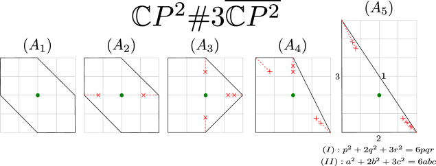
Figure 9. ATBDs of $\mathbb{C}P^{2}\#3\overline{\mathbb{C}P^{2}}$.

3.2. ATFs of $\mathbb{C}P^{2}\#4\overline{\mathbb{C}P^{2}}$

We now see that we have created enough space to perform a toric blowup on the corner (rank 0 singularity) of the 4th or 5th ATBD of Figure 9, in order to obtain an ATF of $\mathbb{C}P^{2}\#4\overline{\mathbb{C}P^{2}}$. We then perform some nodal trades and mutations to, not only create more space for performing another blowup, but also to get the ATBD of triangular shape in Figure 1.

The operations relating each diagram in Figure 10 are described below:

1. Blowup the corner of the ATBD $(A_{5})$ of Figure 9;

2. Applied one nodal trade, getting a $(0,1)$-node;

3. Mutated $(0,1)$-node.

4. Mutated both $(1,-1)$-nodes.

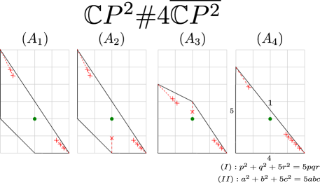
Figure 10. ATBDs of $\mathbb{C}P^{2}\#4\overline{\mathbb{C}P^{2}}$.

3.3. ATFs of $\mathbb{C}P^{2}\#5\overline{\mathbb{C}P^{2}}$

The ATDB of Figure 2, which is a $\pi/2$ rotation of the ATBD $(B_{2})$ in Figure 11. The ATBD $(C_{1})$ in Figure 11 is used to perform another blowup.

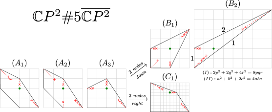
Figure 11. ATBDs of $\mathbb{C}P^{2}\#5\overline{\mathbb{C}P^{2}}$.

The operations relating the $(A)$’s diagrams in Figure 11 are described below:

1. Blowup the corner of the ATBD $(A_{3})$ of Figure 10;

2. Applied one nodal trade, getting a $(0,1)$-node;

3. Mutated $(0,1)$-node.

Following the top arrow towards the $(B)$’s diagrams in Figure 11 we:

1. Mutated both $(0,1)$-nodes and applied one nodal trade, getting a $(1,1)$-node;

2. Mutated all three $(-1,-1)$-nodes.

To obtain $(C_{1})$ ATDB we:

1. Mutated both $(1,0)$-nodes.

3.4. ATFs of $\mathbb{C}P^{2}\#6\overline{\mathbb{C}P^{2}}$

In Figure 12 we show how to get both ATBDs of Figure 2. We could have obtained an ATBD equivalent to the ATBD $(B_{2})$ directly from the ATBD $(A_{3})$, but we will use the ATBD $(B_{1})$ for blowup. We will also perform an almost toric blowup in the ATBD $(C_{2})$.

The operations relating the $(A)$’s diagrams in Figure 12 are described below:

1. Blowup the corner of the ATBD $(C)$ of Figure 11;

2. Applied one nodal trade, getting a $(1,0)$-node;

3. Mutated both $(-1,0)$-nodes.

Following the top arrow towards the $(B)$’s diagrams in Figure 12 we:

1. Mutated the $(0,1)$-node;

2. Mutated all three $(0,-1)$-nodes.

Following the bottom arrow from the $(A_{3})$ ATBD towards the $(C)$’s diagrams in Figure 12 we:

1. Mutated only one $(0,-1)$-node;

2. Mutated all three $(-1,1)$-nodes.

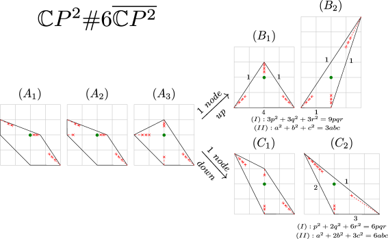
Figure 12. ATBDs of $\mathbb{C}P^{2}\#6\overline{\mathbb{C}P^{2}}$.

3.5. Almost toric blowup

We will next perform a blowup now on a point in lying over a rank 1 elliptic singularity of an ATF, corresponding to an edge of the ATBDs $(B_{1})$ and $(C_{2})$ in Figure 12. That can be done while remaining in the almost toric world.

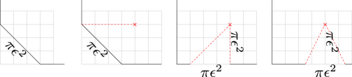
Figure 13. ATBDs on a toric blowup

We first point out that after a toric blowup (1st diagram of Figure 13), we can get ATFs represented by the 2nd, 3rd and 4th ATBDs of Figure 13. See also [Sym, Figures 9,17]. Which makes us think that we can get the 3rd and 4th ATBDs of Figure 13, by applying a blowup on a point over the edge of the 1st ATBD. And indeed we can. In [Aur2, Example 3.1.2], Auroux show how to construct an almost toric fibration on the blowup of $\mathbb{C}^{2}$ over the point $(1,0)$, which lies on the edge of the standard moment polytope of $\mathbb{C}^{2}$. We can than use this almost toric fibration given on the neighborhood of the exceptional divisor as a local model for what we call almost toric blowup. The foollowing proposition is an imediate consequence of [Aur2, Example 3.1.2].

Proposition 3.1 ([Aur2](Example 3.1.2)).

Consider the blowup at $(a,0)\subset\mathbb{C}^{2}$, with symplectic form $\omega_{\epsilon}$, with respect to the standard ball of radius $\epsilon$. There is an ATF on the blowup, with one nodal singularity whose monodromy’s eigendirection is parallel to the direction of the edge (image of the proper transform of the $x$-axis).

The exeptional divisor lives over the segment $R$ on the base of the ATF connecting the node to the edge, in direction “orthogonal to the edge”. Let $\mathcal{N}$ be the pre-image of a neighbourhood of the segment $R$. We can identify the complement of $\mathcal{N}$ with the complement of the pre-image of a similar neighbourhood on the toric moment polytope of $\mathbb{C}^{2}$, as in Figure 14.

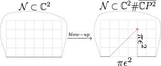
Figure 14. Almost toric blowup.

Proposition 3.2.

Upon the above identification, the ATF of Proposition 3.1 can be made to agree with the toric one of $\mathbb{C}^{2}$ outside $\mathcal{N}$.

Proof.

This follows from the fact that the symplectic form $\omega_{\epsilon}$ agrees with the standard symplectic for of $\mathbb{C}^{2}$ outiside a neighbourhood of the ball of radious $\epsilon$ centered at $(a,0)$. In that region, the tori $L_{r,\lambda}$ described by Auroux in [Aur2, Example 3.1.2] coincides with the standard product torus in $\mathbb{C}^{2}$, i.e., outiside some neighbourhood $\mathcal{N}$ as above, the fibres of the ATF of the blowup are identified with the fibres of the standard moment polytope of $\mathbb{C}^{2}$. ∎

Consider a rank 1 elliptic singularity $p$ of an ATF, lying over an edge of an ATBD. Assume we have segment $R$ starting at (the image of) $p$ embedded inside the ATBD (not crossing a cut or node), orthogonal to the edge containing $p$ and of area $\pi\epsilon^{2}$. Also assume that the area of the edge to the left (or right) of $R$ is bigger than $\pi\epsilon^{2}$ and let $q$ be a point on the edge of distance $\pi\epsilon^{2}$ from (the image of) $p$. Let $S$ be the segment uniting the end point of $R$ with $q$. Consider a symplectomorphism from an almost toric neighborhood of $p$ to the toric neighborhood of a point $(a,0)\subset\mathbb{C}^{2}$. From Propositions 3.1, 3.2 we have:

Proposition 3.3.

There is an ATF on the $\epsilon$-blowup at the point $p$, with ATBD given by replacing a neighbourhood of the base containing the segments $R$ and $S$, by an ATBD with cuts over $R$ and $S$ and a node in their intersection point.

Definition 3.4.

We say that the ATBD on the blowup of Proposition 3.3, is obtained from the previous one via a blowup of length $\pi\epsilon^{2}$.

3.6. ATFs of $\mathbb{C}P^{2}\#7\overline{\mathbb{C}P^{2}}$

In the remaining sections, we refer to the length of an almost toric blowup in a given ATBD according to the grid depicted. Recall that the invariant direction of the monodromy is paralell to the edge containing the point we blowup.

To get the ATBDs $(A_{1})$ and $(D_{1})$ in Figure 15, we apply an almost toric blowup of length $2$ to the ATBDs $(B_{1})$ and $(C_{2})$ of Figure 12. Since $2$ is the distance from the monotone fiber to the bottom edge, it is the area of an Maslov 2 disk lying over the vertical segment. Because it is equal to the area of the exceptional curve, we remain monotone.

After several mutations, we are able to get the ATBDs of Figure 3. As usual, we get ATBDs $(B_{3})$ and $(C_{2})$ to have space for the next blowups.

The operations relating the $(A)$’s diagrams in Figure 15 are described below:

1. Applied an almost toric blowup of length 2 in the edge of the ATBD $(B_{1})$ of Figure 12;

2. Transferred the cut towards the right edge, getting a $(-1,0)$-node;

Following the top arrow towards the $(B)$’s diagrams in Figure 15 we:

1. Mutated only one $(0,-1)$-node;

2. Mutated the $(-1,-1)$-node;

3. Mutated all four $(0,1)$-nodes.

Following the bottom arrow from the $(A_{2})$ ATBD towards the $(C)$’s diagrams in Figure 15 we:

1. Mutated all three $(0,-1)$-nodes;

2. Mutated all six $(0,1)$-nodes.

Now we describe the operations relating the $(D)$’s diagrams in Figure 15:

1. Applied an almost toric blowup of length 2 in the edge of the ATBD $(C_{2})$ of Figure 12;

2. Transferred the cut towards the left edge, getting a $(1,0)$-node;

3. Mutated all six $(1,-1)$-nodes.

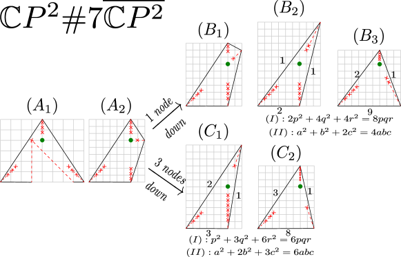
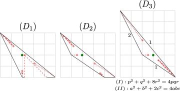
Figure 15. ATBDs of $\mathbb{C}P^{2}\#7\overline{\mathbb{C}P^{2}}$.

3.7. ATFs of $\mathbb{C}P^{2}\#8\overline{\mathbb{C}P^{2}}$

We again blowup on edges of different ATBDs of $\mathbb{C}P^{2}\#7\overline{\mathbb{C}P^{2}}$, namely $(B_{3})$ and $(C_{2})$ in Figure 15. Note that the blowup was not made in the precise format given on Figure 7, but it is equivalent to an honest one (up to nodal slide and change of direction of the cut). After mutations we get the ATBDs of Figure 4.

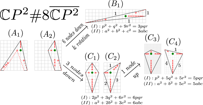
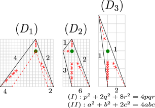
Figure 16. ATBDs of $\mathbb{C}P^{2}\#8\overline{\mathbb{C}P^{2}}$.

The operations relating the $(A)$’s diagrams in Figure 16 are described below:

1. Applied an almost toric blowup of length 6 in the edge of the ATBD $(C_{2})$ of Figure 15;

2. Transferred the cut towards the left edge, getting a $(1,0)$-node;

Following the top arrow towards the $(B)$’s diagrams in Figure 16 we:

1. Mutated all six $(0,-1)$-nodes and applied the counter-clockwise $\pi/2$ rotation $(\in SL(2,\mathbb{Z}))$.

Following the bottom arrow from the $(A_{2})$ ATBD towards the $(C)$’s diagrams in Figure 16 we:

1. Mutated only three $(0,-1)$-nodes;

2. Mutated the $(-1,0)$-node;

3. Mutated only one $(0,1)$-node;

4. Mutated both $(1,0)$-nodes.

Finally, we describe the operations relating the $(D)$’s diagrams in Figure 16:

1. Applied an almost toric blowup of length 6 in the edge of the ATBD $(B_{3})$ of Figure 12 (the grid was refined so the blowup has length 12 on the new grid);

2. Transferred the cut towards the left edge, getting a $(1,0)$-node;

3. Mutated all four $(0,-1)$-nodes.

3.8. ATFs of $\mathbb{C}P^{1}\times\mathbb{C}P^{1}$

We finish by describing the ATBD of triangular shape for $\mathbb{C}P^{1}\times\mathbb{C}P^{1}$ appearring in Figure 1. Apply the counter-clockwise $\pi/2$ rotation $(\in SL(2,\mathbb{Z}))$ to the ATBD $(A_{3})$ of Figure 17 and get the ATBD in Figure 1.

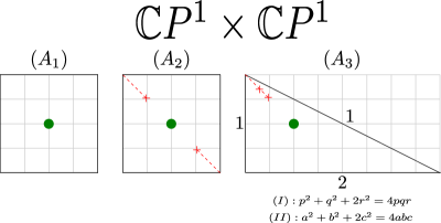
Figure 17. ATBDs of $\mathbb{C}P^{1}\times\mathbb{C}P^{1}$.

1. Standard moment polytope of $\mathbb{C}P^{1}\times\mathbb{C}P^{1}$;

2. Applied two nodal trades, getting a $(-1,1)$ and $(1,-1)$ nodes;

3. Mutated the $(-1,1)$-node.

4. Mutations and ATBDs of triangular shape

Let $\Delta$ be an ATBD of length type $(k_{1}a^{2},k_{2}b^{2},k_{3}c^{2})$, where $(a,b,c)$ are Markov triples for equation (2.2). Assume that $\Delta$ has a monotone fiber (not lying over a cut). Let $\textbf{u}_{1},\textbf{u}_{2},\textbf{u}_{3}$ be primitive vectors in the direction of the edges of $\Delta$, so that $k_{1}a^{2}\textbf{u}_{1}+k_{2}b^{2}\textbf{u}_{2}+k_{3}c^{2}\textbf{u}_{3}=0$. Up to $SL(2,\mathbb{Z})$, we can assume that $\textbf{u}_{3}=(1,0)$. Let $\textbf{w}_{i}$ be the direction of the cut pointing towards the edge whose direction is $\textbf{u}_{i}$, see Figure 18. Let $n_{i}$ be the number of nodes in the cut $\textbf{w}_{i}$. Write $\textbf{w}_{1}=(x,p)$ and $\textbf{w}_{2}=(y,q)$.

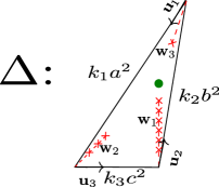
Figure 18. ATBD $\Delta$.

The monodromy around a clockwise oriented loop surrounding $n$ nodes with eigendirection $(s,t)$ is given by [Sym, (4.11)]:

$$\begin{bmatrix}1-st&s^{2}\\ -t^{2}&1+st\end{bmatrix}^{n}=\begin{bmatrix}1-nst&ns^{2}\\ -nt^{2}&1+nst\end{bmatrix}$$ (4.1)

So we have $\textbf{u}_{1}=(1-n_{2}yq,-n_{2}q^{2})$ and $\textbf{u}_{2}=(1+n_{1}xp,n_{1}p^{2})$. Note that $n_{1}p^{2}=|\textbf{u}_{1}\wedge\textbf{u}_{3}|$ and $n_{2}q^{2}=|\textbf{u}_{3}\wedge\textbf{u}_{2}|$, which is invariant under $SL(2,\mathbb{Z})$. So, $|\textbf{u}_{2}\wedge\textbf{u}_{1}|=n_{3}r^{2}$ for some $r\in\mathbb{Z}$.

Proposition 4.1.

We have that:

$$\frac{n_{1}p^{2}}{k_{1}a^{2}}=\frac{n_{2}q^{2}}{k_{2}b^{2}}=\frac{n_{3}r^{2}}{k_{3}c^{2}}$$ (4.2)

We denote the above value by $\lambda$.

Proof.

Follows imediataly from $k_{1}a^{2}\textbf{u}_{1}+k_{2}b^{2}\textbf{u}_{2}+k_{3}c^{2}\textbf{u}_{3}=0$, that $\frac{n_{1}p^{2}}{k_{1}a^{2}}=\frac{n_{2}q^{2}}{k_{2}b^{2}}$. Apply a $SL(2,\mathbb{Z})$ map to conclude that it is also equal to $\frac{n_{3}r^{2}}{k_{3}c^{2}}$. ∎

It also follows from from $k_{1}a^{2}\textbf{u}_{1}+k_{2}b^{2}\textbf{u}_{2}+k_{3}c^{2}\textbf{u}_{3}=0$ and the Markov type II equation that:

$$Kk_{1}k_{2}k_{3}abc=k_{1}a^{2}+k_{2}b^{2}+k_{3}c^{2}=n_{2}yqk_{1}a^{2}-n_{1}xpk_{2}b^{2}$$ (4.3)

It is worth noting that

$$k_{1}aa^{\prime}=k_{2}b^{2}+k_{3}c^{2}$$ (4.4)

Lemma 4.2.

If we mutate all the $\textbf{w}_{1}$-nodes of $\Delta$ we obtain an ATBD of length type $(k_{1}a^{\prime 2},k_{2}b^{2},k_{3}c^{2})$, where $a^{\prime}=Kk_{2}k_{3}bc-a$, i.e., $(a^{\prime},b,c)$ is the mutation of $(a,b,c)$ with respect to $a$. Similarly, if we mutate all $\textbf{w}_{2}\backslash\textbf{w}_{3}$-nodes of $\Delta$, the length type changes according to the mutation of $(a,b,c)$ with respect to $b\backslash c$.

Proof.

We need to prove that the affine length of the edges of the mutated ATBD is proportinal to $(k_{1}a^{\prime 2},k_{2}b^{2},k_{3}c^{2})$. For convinience we rescale the lengths of the edges of $\Delta$ by $a^{\prime}$.

The mutation glue the edges in directions $\textbf{u}_{2}$, $\textbf{u}_{3}$, to get an edge of affine length $a^{\prime}(k_{3}c^{2}+k_{2}b^{2})=ak_{1}a^{\prime 2}$. As in Figure 5, assume we kept $\textbf{w}_{2}$ fixed and mutated $\textbf{w}_{3}$. The mutation divides the edge in direction $\textbf{u}_{1}$ into two edges with affine lengths $\alpha$ and $a^{\prime}k_{1}a^{2}-\alpha$. Say that the edge of length $a^{\prime}k_{1}a^{2}-\alpha$ is opposite to the $w_{2}$-eigenray. It is enough to show that $\alpha=ak_{3}c^{2}$, so $a^{\prime}k_{1}a^{2}-\alpha=a(aa^{\prime}k_{1}-k_{3}c^{2})=ak_{2}b^{2}$.

We have that for some $\beta<0$:

$$a^{\prime}k_{3}c^{2}\textbf{u}_{3}=\beta\textbf{w}_{1}-\alpha\textbf{u}_{1}$$ (4.5)

Hence

$$0=\beta p+\alpha n_{2}q^{2}$$ (4.6)

$$a^{\prime}k_{3}c^{2}=\beta x+\alpha(n_{2}yq-1)$$ (4.7)

By equations (4.2) and (4.7), we have:

$$\beta=-\alpha\frac{n_{2}q^{2}}{p}=-\alpha\frac{k_{2}b^{2}n_{1}p}{k_{1}a^{2}}$$ (4.8)

Plugging into equation (4.7) and using equation (4.3), we get:

$$a^{\prime}k_{3}c^{2} = \frac{\alpha}{a}\left[\frac{1}{k_{1}a}\left(-k_{2}b^{2}n_{1}px+k_{1}a^{2}n_{2}yq\right)-a\right]+\alpha n_{2}q^{2}$$ (4.9)

$$= \frac{\alpha}{a}\left[Kk_{2}k_{3}bc-a\right]=a^{\prime}\frac{\alpha}{a}$$

So indeed $\alpha=ak_{3}c^{2}$.

∎

A direct consequence of Proposition 4.1 and that $\Delta$ is length-related to the Markov type II equation (2.2) is

Corollary 4.3.

Consider the ATBD $\Delta$. The numbers $n_{1}p^{2}=|\textbf{u}_{1}\wedge\textbf{u}_{3}|$, $n_{2}q^{2}=|\textbf{u}_{3}\wedge\textbf{u}_{2}|$, $n_{3}r^{2}=|\textbf{u}_{2}\wedge\textbf{u}_{1}|$ are so that $(p,q,r)$ is a Markov type I triple for the equation:

$$n_{1}p^{2}+n_{2}q^{2}+n_{3}r^{2}=\sqrt{dn_{1}n_{2}n_{3}}pqr,\ \ \eqref{eq: MarkovI}$$

where $d=\frac{K^{2}k_{1}k_{2}k_{3}}{\lambda}$.

It follows then from the Lemma 4.2 and Proposition 4.1:

Corollary 4.4.

If we mutate all the $\textbf{w}_{1}$-nodes of $\Delta$ we obtain an ATBD of node type $((n_{1},p^{\prime}),(n_{2},q),(n_{3},r))$, where $(p^{\prime},q,r)$ is a mutation of the $(p,q,r)$ Markov type I triple. Analogously, for the other $\textbf{w}_{i}$-nodes.

We can verify for each ATBD in Figures 1-4, that the value of $d$ in Corollary 4.3 is equal to the degree of the corresponding del Pezzo. In fact one can prove that Corollary 4.3, without knowing beforhand that the ATBD is length-related to a Markov type II equation (2.2).

Theorem 4.5.

Let $\Delta^{\prime}$ be an ATBD of node type $((n_{1},p),(n_{2},q),(n_{3},r))$, such that the total space $X_{\Delta^{\prime}}$ of the corresponding ATF is monotone. Then $(p,q,r)$ is a Markov type I triple for (2.1).

Proof.

Let $(A,B,C)$ be the length type of $\Delta^{\prime}$. We observe that in Proposition 4.1 still holds, so we have

$$\lambda=\frac{n_{1}p^{2}}{A}=\frac{n_{2}q^{2}}{B}=\frac{n_{3}r^{2}}{C}.$$ (4.10)

We will look at the self-intersection of the anti-canonical divisor class inside the limit orbifold $X_{o}$, as defined in [CR, Che]. The second homology of the limit orbifold $X_{o}$ is one-dimensional, since the moment polytope is a triangle. Denote by $H$ the generator of $H_{2}(X_{o})$.

Claim 4.6.

$X_{o}$ is monotone.

Proof.

Consider a fiber $T$ and disks living over paths conecting $T$ to the edges in the moment polytope of the limit orbifold $X_{o}$. These disks generate $H_{2}(X_{o},T,\mathbb{Q})$, so some integer linear combination is a multiple of $H$ viewed in $H_{2}(X_{o},T,\mathbb{Z})$. Therefore we can complete these disks with a 2-chain in $T$, to get a cycle $m\hat{H}$ representing a multiple of $H$ lying away from the orbifold points.

Now, the complement of small neighbourhoods around the orbifold points can be symplectically embedded into $X_{\Delta^{\prime}}$, up to sliding the nodes close enough to the edges, see [Via2, Figure 7,Section 4.2]. Hence the Chern class and symplectic area of $[m\hat{H}]$ coincide in both $X_{\Delta^{\prime}}$ and $X_{o}$, we get monotonicity for $X_{o}$. ∎

Claim 4.7.

The self-intersection of $H$ is

$$H\cdot H=\frac{1}{\lambda ABC}=\frac{\lambda^{2}}{n_{1}n_{2}n_{3}p^{2}q^{2}r^{2}}.$$ (4.11)

Proof.

The pre-image of the edges of length $A$ and $B$ intersect at one orbifold point and represent $AH,BH\in H_{2}(X_{o})$. The degree of the orbifold point is the determinant of the primitive vectors of the edges, i .e ., $n_{3}r^{2}$. Hence, $AH\cdot BH=1/n_{3}r^{2}$ [CR, Che], and the claim follows. ∎

Now the anti-canonical divisor is represented by the pre-image of the three edges, and its self-intersection is the degree $d$ of $X_{\Delta^{\prime}}$, by the same argument given in Claim 4.6. Therefore, by Claim 4.7:

$$(A+B+C)H\cdot(A+B+C)H=\frac{(A+B+C)^{2}\lambda^{2}}{n_{1}n_{2}n_{3}p^{2}q^{2}r^{2}}=d.$$ (4.12)

Taking the square root and using (4.10), we get the Markov type I equation (2.1).

∎

From Theorem 4.5 and the work of Karpov-Nogin [KN] we see that our list described in Figures 1-4 describes all ATBDs of triangular shape.

Proposition 4.8 (Section 3.5 of [KN]).

All Markov type I equations (2.1) with $n_{1}+n_{2}+n_{3}+d=12$ are the ones appearing in Figures 1, 2, 3, 4.

And from the proposition below and Corollary 4.4, it follows that each ATBD of Figures 1-4, gives rise to infinitely many ones.

Proposition 4.9 (Section 3.7 of [KN]).

Any solution of the Markov type I equations appearing in Figures 1, 2, 3, 4, can be reduced to a minimum solution via a series of mutations. Moreover, for a non-minimum solution 2 mutations increase the sum $p+q+r$ and one reduces.

5. Infinitely many tori

We name $\Theta^{n_{1},n_{2},n_{3}}_{p,q,r}$ the monotone fiber of a monotone ATBD of node-type $((n_{1},p),$ $(n_{2},q),(n_{3},r))$. In this section we show that these tori live in mutually different symplectomorphism classes, completing the proof of Theorem 1.1(a). We also show that there are infinitely many symplectomorphism classes formed by the monotone tori $T_{1}(a,b)$ in $\mathbb{C}P^{2}\#\overline{\mathbb{C}P^{2}}$, depicted in Figure 6, proving 1.1(b). To finish the section we prove Theorem 1.5.

5.1. ATBDs of triangular shape

The Theorem 1.1(a) follows from Theorem 5.1 and the invariance of the boundary Maslov two convex hull for monotone Lagrangian [Via2, Corollary 4.3].

Theorem 5.1.

The boundary Maslov two convex hull of $\Theta^{n_{1},n_{2},n_{3}}_{p,q,r}$ is equal to the convex hull whose vertices are the primitive vectors generating the fan of the corresponding limit orbifold. Moreover, the affine length of the edges of $\mho_{\Theta^{n_{1},n_{2},n_{3}}_{p,q,r}}$ is $n_{1}p,n_{2}q,n_{3}r$.

Proof.

The proof of the first part is totally analogous to the proof of Theorem 1.1 [Via2, Section 4], so we will only sketch here. Denote by $M$ the del Pezzo surface and $\overline{M_{+}^{\infty}}$ the limit orbifold.

We first consider contact submanifolds $V_{i}$’s bounding the symplectic submanifols $M_{-i}$’s formed by the pre-image of an open sector of the ATBD that encloses $n_{i}$ nodes, $i=1,2,3$. We embed $M_{+}=M\setminus(M_{-1}\cup M_{-2}\cup M_{-3})$ inside the limit orbifold. We pull back the complex form from the orbifold to $M_{+}$ and extend it to $M$. We also pullback the Maslov index 2 holomorphic discs $\alpha,\beta,\gamma$ [CP], which live in the complement of the orbifold points in the limit orbifold. The boundary of their homology classes corresponds to the primitive vectors generating the fan of $\overline{M_{+}^{\infty}}$, and they will give rise to the vertices of $\mho_{\Theta^{n_{1},n_{2},n_{3}}_{p,q,r}}$.

Given an pseudo-holomorphic disk $u$ with boundary on $\Theta^{n_{1},n_{2},n_{3}}_{p,q,r}$, we look at its limit under neck-streching, which is at the pseudo-holomorphic building [BEH⁺, EGH]. The part of the pseudo-holomorphic building lying in $M_{+}^{\infty}$, compactifyies to a degenerated pdeudo-holomorphic disk $u^{\infty}_{+}$ in the limit orbifold $\overline{M_{+}^{\infty}}$, having the same boundary as $u$ upon identification of $\Theta^{n_{1},n_{2},n_{3}}_{p,q,r}$ as a fiber in the limit orbifold.

We have that $[u^{\infty}_{+}]$ intersects positively each of the classes of the pre-images $A,B,C$ of the edges of the limit orbifold. Indeed, consider a component of $[u^{\infty}_{+}]$, either is not a multiple of $A$, and hence intersects $A$ non-negatively [CR, Che], or it is a positive multiple of $A$, which has positive self intersection, see Claim 4.7. Similar for intersection with $B$ and $C$.

Since each disk $\alpha,\beta$ or $\gamma$ intersects only one of the divisors $A,B,C$, and the plane of Maslov index 2 classes in the orbifold projects injectively to $H_{1}(\Theta^{n_{1},n_{2},n_{3}}_{p,q,r})$ under the boundary map, we can conclude the first part of the Theorem.

For the second part, we use the notation in the description of $\Delta$ in Section 4, see Figure 18. The primitive vectors for the fan of the limit orbifold are $\textbf{v}_{3}=(0,1)$, $\textbf{v}_{1}=(n_{2}q^{2},1-n_{2}yq)$, $\textbf{v}_{2}=(n_{1}p^{2},-n_{1}xp-1)$, which are orthogonal to $\textbf{u}_{3}$, $\textbf{u}_{1}$, $\textbf{u}_{2}$. Hence the affine length of the edges $\textbf{v}_{1}-\textbf{v}_{3}=n_{2}q(q,-y)$ and $\textbf{v}_{2}-\textbf{v}_{3}=n_{2}p(p,-x)$ are respectively $n_{2}q$ and $n_{1}p$. After applying a $SL(2,\mathbb{Z})$ map, we can do the same analysis to conclude that the affine length of the edge $\textbf{v}_{1}-\textbf{v}_{2}$ is $n_{3}r$. ∎

5.2. On $\mathbb{C}P^{2}\#\overline{\mathbb{C}P^{2}}$

This section is devoted to prove Theorem 1.1(b). We start with ATBDs of $\mathbb{C}P^{2}$ wiht two nodes and one corner (rank 0 elliptic singularity) of length-type $(a^{2},b^{2},1)$, where $a^{2}+b^{2}+1=3ab$. We assume $a<b$, and scale the symplectic form so that the affine length of the edges are $3$, $3a^{2}$, $3b^{2}$. We need to blow up so that the are of the exceptional divisor $E$ is 1/3 of the area of the line. The area of the anti-canonical divisor $3[\mathbb{C}P^{1}]$, represented by the preimage of the edges of the ATBD [Sym], is $3a^{2}+3b^{2}+1=9ab$. Hence we blow up so that the symplectic area $\omega\cdot E=ab$. See Figure 6. We note we have space to blowup, since $3a^{2}-ab=ab^{\prime}>0$ and $3b^{2}-ab=ba^{\prime}>0$. We name the monotone torus $T_{1}(a,b)$.

We proceed as in the proof of Theorem 5.1, were we apply neck-stretching “degenerating” the ATBD towards its limit orbifold. We will use similar notation.

Let’s name $\alpha$, $\beta$, $\gamma$, $\varepsilon$ the classes of holomorphic disks living in the complement of the orbifold points of the limit orbifold $\overline{M^{\infty}_{+}}$. We consider a pseudo-holomorphic disk $u$ with boundary on $T_{1}(a,b)$, and we look at the degenerate pseudo-holomorphic disk $u_{+}^{\infty}$ in the limit orbifold $\overline{M^{\infty}_{+}}$, which is the compactification of the top building of the neck-stretch limit.

We name $A$, $B$, $C$, the pre-image of the edges of the limit orbifold whose symplectic area are respectively $3a^{2}-ab$, $3b^{2}-ab$, and $3$. We keep calling $E$ the class of limit of the exceptional curve in the limit orbifold. Say that $\alpha$ intesects $A$, $\beta$ intesects $B$, $\gamma$ intesects $C$ and $\varepsilon$ intesects $E$.

Proposition 5.2.

We have that $A\cdot A=\frac{a^{2}-b^{2}}{b^{2}}<0$, $B\cdot B=\frac{b^{2}-a^{2}}{a^{2}}>0$ $C\cdot C=\frac{1}{a^{2}b^{2}}>0$, $E\cdot E=-1<0$.

Proof.

Use the formula

$$D\cdot D=\frac{|\textbf{w}\wedge\textbf{v}|}{|\textbf{v}\wedge\textbf{u}||\textbf{w}\wedge\textbf{u}|},$$

where $D$ is represented by an edge of the moment polytope of a tori orbifold with primitive vector u, and such that the primitive vectors of the adjacent edges are v and w. We also have that u points from the v-edge to the w-edge and $|\textbf{v}\wedge\textbf{u}|>0$.

An alternative proof is to use that $A+E=a^{2}C$, $B+E=b^{2}C$ and arguments similar to Claim 4.7. ∎

So the positivity of intersection argument given in the proof of Theorem 5.1 fails. Nonetheless we have:

Lemma 5.3.

The intesrsections $E\cdot[u^{\infty}_{+}]\geq 0$, $B\cdot[u^{\infty}_{+}]\geq 0$ and $C\cdot[u^{\infty}_{+}]\geq 0$.

Proof.

That $C\cdot[u^{\infty}]\geq 0$ and $B\cdot[u^{\infty}_{+}]\geq 0$ follows as before, since a component of $u^{\infty}_{+}$ contributing negatively to $C\cdot[u^{\infty}]$ would have to be a positive multiple of $C$, but $C\cdot C>0$. Similar for $B$ (in fact no component could be a multiple of $B$ by area reasons).

That $E\cdot[u^{\infty}_{+}]\geq 0$ follows from $\omega^{\infty}_{+}\cdot E=\omega^{\infty}_{+}\cdot[u^{\infty}_{+}]=ab$. Since $u^{\infty}_{+}$ has the ‘main component’ with boundary on (the limit of) $T_{1}(a,b)$, and all components have positive symplectic area, we can’t have a multiple of $E$.

∎

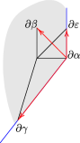
Figure 19. $\partial\alpha$ is a corner of $\mho_{T_{1}(a,b)}$.

Lemma 5.4.

Upon identification of $T_{1}(a,b)$ with its limit in the limit orbifold, we have that $\partial\alpha$ is a corner of the boundary Maslov-2 convex hull $\mho_{T_{1}(a,b)}$.

Proof.

First we notice that the count of pseudo-holomporphic disk in the class $\alpha$ is $\pm 1$, by the same arguments as in [Via2, Lemma 4.11].

The classes of Maslov index 2 (or symplect area $ab$) disks with boundary in (the limit of) $T_{1}(a,b)$ inside the limit orbifold must be of the form:

$$\alpha+k(\varepsilon-\alpha)+l(\beta-\alpha)+m(\gamma-\alpha)$$ (5.1)

By Lemma 5.3, we see that the class $[u^{\infty}_{+}]$ must have $k,l,m\in\mathbb{Z}_{\geq 0}$ in (5.1). Hence $\partial\alpha$ is a corner of $\mho_{T_{1}(a,b)}$, see Figure 19.

∎

Lemma 5.5.

The affine angle of the corner $\partial\alpha$ in $\mho_{T_{1}(a,b)}$,  i. e., the norm of the determinant of the primitive vectors of the edges of the corner, is $b^{\prime}=3a-b$.

Proof.

We identify $\partial\alpha=(1,0)$, $\partial\beta=(0,1)$, $\partial\epsilon=(1,1)$, $(-a^{2},-b^{2})$. Recall that $1+a^{2}=bb^{\prime}$. Hence $\partial\gamma-\partial\alpha=-b(b^{\prime},b)$. Therefore the primitive vectors are $(0,1)$ and $(b^{\prime},b)$. ∎

Lemma 5.6.

The Maslov-2 convex hull $\mho_{T_{1}(a,b)}$ is compact.

Proof.

By area reasons, there is a constant $N_{0}\in\mathbb{Z}_{>0}$ such that $[u_{+}\infty]$ cannot have $N_{0}$ or more components in the class $A$, for all pseudo-holomorphic disks $u$. Therefore, there is a constant $N\in\mathbb{Z}_{>0}$ such that $A\cdot[u_{+}\infty]>-N$. So, $k+l+m<N+1$ in the decomposition (5.1) of $[u_{+}\infty]$, which implies the Lemma. ∎

Recall that two Maslov-2 convex hull are equivalent if they are related via $SL(2,\mathbb{Z})$. Since we have an infinite number of values of affine angles, the number of equivalence classes for the Maslov-2 convex hulls $\mho_{T_{1}(a,b)}$s cannot be finite. This finishes the proof of Theorem 1.1(b).

5.3. Proof of Theorem 1.5

Let $(X,\omega)$ be a del Pezzo surface and consider $\Theta^{n_{1},n_{2},n_{3}}_{p,q,r}\subset X$ the monotone Lagrangian tori described in this Section 5. If one applies nodal slide along a segment $[A,B]$ inside the base of an ATF, the new ATF can be chosen to be equal to the previous one outside a small neighbourhood of $[A,B]$. Therefore, we may assume that, provided we apply nodal trade for all nodes beforhand, over the edge of all the ATFs desbribed in Section 3 for the del Pezzo surface $X$ lives the same symplectic torus $\Sigma$. Also, all the monotone Lagrangian tori $\Theta^{n_{1},n_{2},n_{3}}_{p,q,r}$ live in $X\setminus\Sigma$.

Let $V=\partial X$. In a neighbourhood of $V$, there is a Liouville vector field pointing outside $V$ for which the corresponding Reeb vector field $R\subset\Gamma(TV)$ is so that $\nicefrac{{V}}{{R}}\cong\Sigma$. Therefore we may attach the positive symplectization of $V$ to $X\setminus\Sigma$, and see $\Theta^{n_{1},n_{2},n_{3}}_{p,q,r}\subset(X\setminus\Sigma)\cup(V\times[0,+\infty))$ as a fiber of an ATF. It follows from seeing $X\setminus\Sigma$ coming from Weinstein handle attachments to the co-disk bundle $D^{*}_{\epsilon}\Theta^{n_{1},n_{2},n_{3}}_{p,q,r}$ along the boundary of Lagrangian disks, that $\Theta^{n_{1},n_{2},n_{3}}_{p,q,r}$ are exact in $(X\setminus\Sigma)\cup(V\times[0,+\infty))$, see Section 6.1.

Theorem (1.5).

The tori $\Theta^{n_{1},n_{2},n_{3}}_{p,q,r}\subset(X\setminus\Sigma)\cup(V\times[0,+\infty))$ belong to mutually different Hamiltonian isotopy classes.

Proof.

If there were a Hamiltonian isotopy between two of these tori, it could be made to be identity outside $(X\setminus\Sigma)\cup(V\times[0,C))$, for some constant $C$. Therefore it is enough to prove that the tori are not Hamiltonian isotopic in the del Pezzo surface $(X,\omega_{C})$, obtained by collapsing the Reeb vector field inside $V\times\{C\}$. In other words, $(X,\omega_{C})$ is obtained by inflating $X$ along $\Sigma$ by a factor of $C$. We note that $\Sigma\subset X$ not only represents the Poincaré dual to $\mathrm{c}_{1}$, but as a cycle in $X\setminus\Theta^{n_{1},n_{2},n_{3}}_{p,q,r}$, it represents the Poincaré dual to half of the Maslov class $\mu/2\in H^{2}(X,\Theta^{n_{1},n_{2},n_{3}}_{p,q,r})$. Looking at the ATF in $(X\setminus\Sigma)\cup(V\times[0,C)$ we see that, not only $\Theta^{n_{1},n_{2},n_{3}}_{p,q,r}\subset(X,\omega_{C})$ remains monotone, it is the monotone fiber of an ATBD of $(X,\omega_{C})$, which is the corresponding multiple of the initial ATBD of $(X,\omega)$. Hence the tori $\Theta^{n_{1},n_{2},n_{3}}_{p,q,r}$ are mutually non-Hamiltonian isotopic in $(X,\omega_{C})$.

∎

Remark 5.7.

Note that taking the complement of the divisor that is Poincaré dual to a multiple of the Maslov class for all tori was essential. All Lagrangian tori constructed in $\mathbb{C}P^{2}$ can be shown to live in the complement of a line. But Dimitroglou Rizzel’s classification of tori in $\mathbb{C}^{2}$ [DR] shows that there are only Clifford and Chekanov monotone Lagrangian tori in $\mathbb{C}^{2}$, up to Hamiltonian isotopy.

6. Relating to other works

6.1. Shende-Treumann-Williams

Consider a surface $S$ and a closed circle $\sigma\subset S$. Let $M=D^{*}S$ the co-disk bundle of $S$ (with respect to some auxiliary metric on $S$). We can lift $\sigma$ to a Legendrian $\sigma^{\prime}\subset\partial M$, by considering over each point $s\in\sigma$ the co-vector that vanishes on the tangent vectors of $\sigma$ at $s$. We can then attach a Weinstein handle along $\sigma^{\prime}$ obtaining a new Liouville manifold $M_{\sigma}$. Shende-Treumann-Williams show that there is a way to “mutate” the surface $S$ by sliding it along the Lagrangian core $L_{\sigma^{\prime}}$ of the Weinstein handle, obtaining a new exact Lagrangian $S^{\sigma}$. We also note that $M_{\sigma}$ is homotopic equivalent to $S\cup L_{\sigma}$, where $L_{\sigma}$ is a Lagrangian disk with boundary $\sigma\subset S$ given by the continuation of the Lagrangian core $L_{\sigma^{\prime}}$ where we shrink the length of the co-vectors of $\sigma^{\prime}$ to zero.

This idea can be generalized for any number of cycles $\sigma_{1},\dots,\sigma_{n}$ in $S$, where we obtain a Lioville manifold $M_{\sigma_{1},\dots,\sigma_{n}}$, with a Lagrangian skeleton given by $S\cup L_{\sigma_{1}}\cdots\cup L_{\sigma_{n}}$, where $L_{\sigma_{i}}$ is a Lagrangian disk with boundary on $\sigma_{i}$. Also, for any word $w$ on $\sigma_{1},\dots,\sigma_{n}$, one can obatain a surface $S^{w}$ mutated along Lagrangian disks according to the word $w$. Moreover, Shende-Treumann-Williams show how to also mutate the Lagrangian disks, to obtain Lagrangians disks $L^{w}_{\sigma^{w}_{i}}$’s with boundary on $S^{w}$ so that $M_{\sigma_{1},\dots,\sigma_{n}}$ has $S^{w}\cup L^{w}_{\sigma^{w}_{1}}\cdots\cup L^{w}_{\sigma^{w}_{n}}$ as a Lagrangian skeleton. They also show how these mutations can be encoded using cluster algebra.

Question 6.1.

Do the $S^{w}$’s give infinitely many Hamiltonian isotopy classes in $M_{\sigma_{1},\dots,\sigma_{n}}$ among exact Lagrangians?

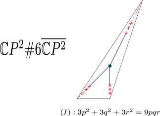
Figure 20. The complement of an anti-canonical surface in $\mathbb{C}P^{2}\#6\overline{\mathbb{C}P^{2}}$ as a result of attaching nine Lagrangian disks to the central fiber.

When $S$ is a torus $T$, this is precisely what is happening in the complement of the anti-canonical surface $\Sigma$ living over the edge of the base of the monotone ATFs. In fact in [TV1], we show that if the cycles $\sigma_{i}$’s are taken to be periodic orbits of the self torus action of $T$, then we obtain an ATF on $M_{\sigma_{1},\dots,\sigma_{n}}$. Moreover, the ATF can be represented by an ATBD whose cuts points towards the image of $T$ and are in the direction of the cycles $\sigma$ via the identification $H_{1}(T,\mathbb{R})$ with $\mathbb{R}^{2}\supset$ ATBD. The Lagrangian disks live over the segment uniting $T$ with the cuts, see Figure 20. In that way, the torus $T^{w}$ mutated with respect to a word $w$ on $\sigma_{1},\dots,\sigma_{n}$ corresponds to sliding the nodes over the central fiber according to $w$. Also, if each time we slide a node through the central fiber we perform a mutation on the ATBD, the mutated Lagrangians $L^{w}_{\sigma^{w}_{i}}$’s can be read from the cuts of the mutated ATBD.

Figure 20 illustrates $\mathbb{C}P^{2}\#6\overline{\mathbb{C}P^{2}}\setminus\Sigma$, where we have nine Lagrangian disks living over the segments connecting the central fiber to each of the nodes of the ATBD. Theorem 1.5 shows that total mutations give rise to tori $\Theta^{3,3,3}_{p,q,r}$ living in mutually distinct Hamiltonian isotopy classes.

6.2. Keating

In [Kea2, Proposition 5.21], Keating shows how the Milnor fibers

$$\mathcal{T}_{3,3,3}=\{x^{3}+y^{3}+z^{3}+1=0\};$$

$$\mathcal{T}_{2,4,4}=\{x^{2}+y^{4}+z^{4}+1=0\};$$

$$\mathcal{T}_{2,3,6}=\{x^{2}+y^{3}+z^{6}+1=0\};$$

compactify respectivelly to the del Pezzo surfaces $\mathbb{C}P^{2}\#6\overline{\mathbb{C}P^{2}}$, $\mathbb{C}P^{2}\#7\overline{\mathbb{C}P^{2}}$, $\mathbb{C}P^{2}\#8\overline{\mathbb{C}P^{2}}$.

Also, in [Kea1, Section 7.4], Keating describes how the Milnor fibers $\mathcal{T}_{p,q,r}$ of $x^{p}+y^{q}+z^{r}+axyz$ can be obtained by attaching $p,q,r$ Weinstein handles to $D^{*}T$ along Legendrian lifts of three circles, mutually intersecting at one point. By our discussion on the precious section, we see the compactifications described in [Kea2, Proposition 5.21] depicted in Figures 12$(B_{2})$, 15$(B_{2})$, 16$(C_{2})$.

As a consequence of Theorem 1.5, we have that there are infinitely many exact Lagrangian tori in $\mathcal{T}_{3,3,3},\mathcal{T}_{2,4,4},\mathcal{T}_{2,3,6}$.

6.3. Karpov-Nogin and Hacking-Prokhorov

There seems to be a relation between $m$-block collection of sheaves [KN] on a del Pezzo surface and its ATBDs. By the Theorem in [KN, Section 3], a $3$-block collection on a degree $d$ del Pezzo suface containing exceptional collections with $n_{1}$,$n_{2}$,$n_{3}$ sheaves of ranks $p,q,r$, satisfy the Markov type one equation (2.1).

Question 6.2.

Suppose we have an ATBD with node type $((n_{1},p_{1}),\cdots,(n_{m},p_{m}))$ of a del Pezzo surface. Is there an $m$-block collection $(\mathcal{E}_{1},\cdots,\mathcal{E}_{m})$, so that the exeptional colection $\mathcal{E}_{i}$ contains $n_{i}$ sheaves of rank $p_{i}$?

There is also a relation between $\mathbb{Q}$-Gorenstein smoothing [HP] and ATBD on the smooth surface. In [HP, Theorem 1.2], it is shown that the weighted projective planes that admits a $\mathbb{Q}$-Gorenstein smoothing are precisely the ones given by the limit orbifolds of the ATBDs obtianed by total mutation of the ones in Figure 1. It seems that pushing the nodes towards the edges of an ATBD corresponds to degenerating the del Pezzo surface to the limit orbifold.

Question 6.3.

Do monotone Lagrangians of a del Pezzo know about its degenerations? In other words, do the limit orbifold of an ATBD has a $\mathbb{Q}$-Gorenstein smoothing to the corresponding del Pezzo?

6.4. FOOO and Wu

The singular fibration of $\mathbb{C}P^{1}\times\mathbb{C}P^{1}$ described in [FOOO3] can be thought as a degeneration of the ATBD $(A_{3})$ of Figure 17 where both nodes aproach the edge, but instead of degenerating to an orbifold point, a Lagrangian sphere that lives between the nodes survive, see [TV2, Remark 3.1]. Similarly, the ATBD of $\mathbb{C}P^{2}$ with limit orbifold $\mathbb{C}P(1,1,4)$, can be thought to degenerate to the singular fibration described in [Wu], where instead of an orbifold point we have a Lagrangian $\mathbb{R}P^{2}$.

A way to see this degenerations is using the auxiliary Lefschetz fibration which compactifies $(x,y)\in\mathbb{C}^{2}\mapsto xy\in\mathbb{C}$ to $\mathbb{C}P^{1}\times\mathbb{C}P^{1}\backslash\mathbb{C}P^{2}$ to get ATFs, as in [Aur1, Aur2]. A (possibly singular) Lagrangian torus is the union of orbits of the $S^{1}$-action $e^{i\phi}\cdot(x,y)=(e^{i\phi}x,e^{-i\phi}y)$ with the same moment image, living over a circle in the base. A Lagrangian $S^{2}\backslash\mathbb{R}P^{2}$ lives over the segment $\mathbb{R}_{\geq 0}\cup\{\infty\}$ and is formed by orbits of the $S^{1}$-action with moment image $0$. Consider a continuous family of foliations $\mathcal{F}_{t}$, $t\in[0,\epsilon)$, of the base $\mathbb{C}P^{1}$ so that: for $t\neq 0$, $\mathcal{F}_{t}$ is formed by circles degenerating to the points $-1$ and $1$; and $\mathcal{F}_{0}$ is formed by circles degenerating to the point $-1$ and the segment $\mathbb{R}_{\geq 0}\cup\{\infty\}$. The ATF of $\mathbb{C}P^{1}\times\mathbb{C}P^{1}\backslash\mathbb{C}P^{2}$ is formed by Lagrangian tori living over some folliation $\mathcal{F}_{\delta}$ for a small $\delta$. The singular fibration described in [FOOO3] $\backslash$ [Wu] can be interpreted as a singular Lagrangian fibration, where each Lagrantian is given by the orbits of the $S^{1}$-action with moment image $\mu$ living over each leave of the folliation $\mathcal{F}_{\mu}$, if $\mu\leq\delta$, and living ove the fibration $\mathcal{F}_{\delta}$ for $\mu\geq\delta$. So, for $\mu=0$, we get a family of Lagrangian tori, projecting to the circles of $\mathcal{F}_{0}$, degenerating to $S^{1}$ at one end and to a Lagrangian $S^{2}\backslash\mathbb{R}P^{2}$ at the other.

The point is: in [FOOO3] it is shown that there is a continuum of non-displaceable fibers of the singular fibration described. It follows that there is a continuum of non-displaceable fibers on the ATBD $(A_{3})$ of Figure 17. The non-displaceability of the analougous fibers for the $\mathbb{C}P^{2}$ case is an open question. A more general question is:

Question 6.4.

Which of the ATBDs described in this paper have a continuum of non-displaceable fibers?

References

- [Aur1] D. Auroux. Mirror symmetry and T-duality in the complement of an anticanonical divisor. J. Gökova Geom. Topol., 1:51–91, 2007.
- [Aur2] D. Auroux. Special Lagrangian fibrations, wall-crossing, and mirror symmetry. In Surveys in differential geometry. Vol. XIII. Geometry, analysis, and algebraic geometry: forty years of the Journal of Differential Geometry, volume 13 of Surv. Differ. Geom., pages 1–47. Int. Press, Somerville, MA, 2009.
- [BEH+] F. Bourgeois, Y. Eliashberg, H. Hofer, K. Wysocki, and E. Zehnder. Compactness results in Symplectic Field Theory. Geom. Topol., 7:799–888, 2003.
- [Che] W. Chen. Orbifold adjunction formula and symplectic cobordisms between lens spaces. Geom. Topol., 8:701–734 (electronic), 2004.
- [CP] H. Cho, C and M. Poddar. Holomorphic orbi-discs and Lagrangian Floer cohomology of symplectic toric orbifolds. J. Differential Geom., 98(1):21–116, 2014.
- [CR] W. Chen and Y. Ruan. Orbifold Gromov-Witten theory. In Orbifolds in mathematics and physics (Madison, WI, 2001), volume 310 of Contemp. Math., pages 25–85. Amer. Math. Soc., Providence, RI, 2002.
- [DR] G. Dimitroglou Rizell. The Classification of Lagrangian tori in a four-dimensional symplectic vectorspace. In preparation.
- [EGH] Y. Eliashberg, A. Givental, and H. Hofer. Introduction to Symplectic Field Theory. In Visions in Mathematics, pages 560–673. Birkhäuser, 2010.
- [EP] Yakov Eliashberg and Leonid Polterovich. Unknottedness of Lagrangian surfaces in symplectic -manifolds. Internat. Math. Res. Notices, (11):295–301, 1993.
- [FOOO1] K. Fukaya, Y.-G. Oh, H. Ohta, and K. Ono. Lagrangian Intersection Floer Theory: Anomaly and Obstruction, volume 46 of Stud. Adv. Math. American Mathematical Society, International Press, 2010.
- [FOOO2] K. Fukaya, Y.-G. Oh, H. Ohta, and K. Ono. Lagrangian Floer theory on compact toric manifolds II: bulk deformations. Selecta Math. (N.S.), 17(2):609–711, 2011.
- [FOOO3] K. Fukaya, Y.-G. Oh, H. Ohta, and K. Ono. Toric Degeneration and Nondisplaceable Lagrangian Tori in . Internat. Math. Res. Notices, 13:2942–2993, 2012.
- [Gro] M. Gromov. Pseudo holomorphic curves in symplectic manifolds. Invent. Math., 82:307–347, 1985.
- [GU] S. Galkin and A. Usnich. Laurent phenomenon for landau-ginzburg potential. available at http://research.ipmu.jp/ipmu/sysimg/ipmu/417.pdf, 2010.
- [HP] P. Hacking and Y. Prokhorov. Smoothable del Pezzo surfaces with quotient singularities. Compos. Math., 146(1):169–192, 2010.
- [Kea1] A. Keating. Homological mirror symmetry for hypersurface cusp singularities. arXiv:1510.08911, 2015.
- [Kea2] A. Keating. Lagrangian tori in four-dimensional Milnor fibres. Geom. Funct. Anal., 25(6):1822–1901, 2015.
- [KN] B. V. Karpov and D. Y. Nogin. Three-block exceptional sets on del Pezzo surfaces. Izv. Ross. Akad. Nauk Ser. Mat., 62(3):3–38, 1998.
- [Laz] L. Lazzarini. Existence of a somewhere injective pseudo-holomorphic disc. Geom. Funct. Anal., 10(4):829–862, 2000.
- [LS] N. C. Leung and M. Symington. Almost toric symplectic four-manifolds. J. Symplectic Geom., 8(2):143–187, 2010.
- [McD1] D. McDuff. The structure of rational and ruled symplectic -manifolds. J. Amer. Math. Soc., 3(3):679–712, 1990.
- [McD2] Dusa McDuff. From symplectic deformation to isotopy. In Topics in symplectic -manifolds (Irvine, CA, 1996), First Int. Press Lect. Ser., I, pages 85–99. Int. Press, Cambridge, MA, 1998.
- [MS] D. McDuff and D. A. Salamon. Introduction to symplectic topology. Oxford Mathematical Monographs. 1998.
- [OO1] H. Ohta and K. Ono. Notes on symplectic -manifolds with . II. Internat. J. Math., 7(6):755–770, 1996.
- [OO2] H. Ohta and K. Ono. Symplectic -manifolds with . In Geometry and physics (Aarhus, 1995), volume 184 of Lecture Notes in Pure and Appl. Math., pages 237–244. Dekker, New York, 1997.
- [Sal] D. Salamon. Uniqueness of symplectic structures. Acta Math. Vietnam., 38(1):123–144, 2013.
- [STW] V. Shende, D. Treumann, and H. Williams. Cluster varieties and Symplectic 4-manifolds. In preparation.
- [Sym] M. Symington. Four dimensions from two in symplectic topology. In Topology and geometry of manifolds (Athens, GA, 2001), volume 71 of Proc. Sympos. Pure Math., pages 153–208. Amer. Math. Soc., Providence, RI, 2003.
- [Tau1] C. H. Taubes. The Seiberg-Witten and Gromov invariants. Math. Res. Lett., 2(2):221–238, 1995.
- [Tau2] C. H. Taubes. : from the Seiberg-Witten equations to pseudo-holomorphic curves. J. Amer. Math. Soc., 9(3):845–918, 1996.
- [Tau3] C. H. Taubes. Seiberg Witten and Gromov invariants for symplectic -manifolds, volume 2 of First International Press Lecture Series. International Press, Somerville, MA, 2000. Edited by Richard Wentworth.
- [TV1] D. Tonkonog and R. Vianna. In preparation.
- [TV2] D. Tonkonog and R. Vianna. Low-area Floer theory and non-displaceability. arXiv:1511.00891, 2015.
- [Via1] R. Vianna. On exotic Lagrangian tori in . arXiv:1305.7512, 2013.
- [Via2] R. Vianna. Infinitely many exotic monotone Lagrangian tori in . arXiv:1409.2850, 2014.
- [Wu] W. Wu. On an exotic Lagrangian torus in . Compositio Math., 151(7):1372–1394, 2015.