A Theory of Generative ConvNet
Abstract
We show that a generative random field model, which we call generative ConvNet, can be derived from the commonly used discriminative ConvNet, by assuming a ConvNet for multi-category classification and assuming one of the categories is a base category generated by a reference distribution. If we further assume that the non-linearity in the ConvNet is Rectified Linear Unit (ReLU) and the reference distribution is Gaussian white noise, then we obtain a generative ConvNet model that is unique among energy-based models: The model is piecewise Gaussian, and the means of the Gaussian pieces are defined by an auto-encoder, where the filters in the bottom-up encoding become the basis functions in the top-down decoding, and the binary activation variables detected by the filters in the bottom-up convolution process become the coefficients of the basis functions in the top-down deconvolution process. The Langevin dynamics for sampling the generative ConvNet is driven by the reconstruction error of this auto-encoder. The contrastive divergence learning of the generative ConvNet reconstructs the training images by the auto-encoder. The maximum likelihood learning algorithm can synthesize realistic natural image patterns.
1 Introduction
The convolutional neural network (ConvNet or CNN) (LeCun et al., 1998; Krizhevsky et al., 2012) has proven to be a tremendously successful discriminative or predictive learning machine. Can the discriminative ConvNet be turned into a generative model and an unsupervised learning machine? It would be highly desirable if this can be achieved because generative models and unsupervised learning can be very useful when the training datasets are small or the labeled data are scarce. It would also be extremely satisfying from a conceptual point of view if both discriminative classifier and generative model, and both supervised learning and unsupervised learning, can be treated within a unified framework for ConvNet.
In this conceptual paper, we show that a generative random field model, which we call generative ConvNet, can be derived from the commonly used discriminative ConvNet, by assuming a ConvNet for multi-category classification and assuming one of the categories is a base category generated by a reference distribution. The model is in the form of exponential tilting of the reference distribution, where the exponential tilting is defined by the ConvNet scoring function. If we further assume that the non-linearity in the ConvNet is Rectified Linear Unit (ReLU) (Krizhevsky et al., 2012) and that the reference distribution is Gaussian white noise, then we obtain a generative ConvNet model that is unique among energy-based models: The model is piecewise Gaussian, and the means of the Gaussian pieces are defined by an auto-encoder, where the filters in the bottom-up encoding become the basis functions in the top-down decoding, and the binary activation variables detected by the filters in the bottom-up convolution process become the coefficients of the basis functions in the top-down deconvolution process Zeiler & Fergus (2014). The Langevin dynamics for sampling the generative ConvNet is driven by the reconstruction error of this auto-encoder. The contrastive divergence learning (Hinton, 2002) of the generative ConvNet reconstructs the training images by the auto-encoder. The maximum likelihood learning algorithm can synthesize realistic natural image patterns.
The main purpose of our paper is to explore the properties of the generative ConvNet, such as being piecewise Gaussian with auto-encoding means, where the filters in the bottom-up operation take up a new role as the basis functions in the top-down representation. Such an internal representational structure is essentially unique among energy-based models. They are the results of the marriage between the piecewise linear structure of the ReLU ConvNet and the Gaussian white noise reference distribution. The auto-encoder we elucidate is a harmonious fusion of bottom-up convolution and top-down deconvolution.
The reason we choose Gaussian white noise as the reference distribution is that it is the maximum entropy distribution with given marginal variance. Thus it is the most featureless distribution. Another justification for the Gaussian white noise distribution is that it is the limiting distribution if we zoom out any stochastic texture pattern, due to the central limit theorem Wu et al. (2008). The ConvNet seeks to search for non-Gaussian features in order to recover the non-Gaussian distribution before the central limit theorem takes effect. Without the Gaussian reference distribution that contributes the norm term to the energy function, we will not have the auto-encoding form in the internal representation of the model. In fact, without Gaussian reference distribution, the density of the model is not even integrable. The Gaussian reference distribution is also crucial for the Langevin dynamics to be driven by the reconstruction error.
The ReLU is the most commonly used non-linearity in modern ConvNet (Krizhevsky et al., 2012). It makes the ConvNet scoring function piecewise linear Montufar et al. (2014). Without the piecewise linearity of the ConvNet, we will not have the piecewise Gaussian form of the model. The ReLU is the source of the binary activation variables because the ReLU function can be written as , where is the binary variable indicating whether or not. The binary variable can also be derived from the derivative of the ReLU function. The piecewise linearity is also crucial for the exact equivalence between the gradient of the contrastive divergence learning and the gradient of the auto-encoder reconstruction error.
2 Related Work
The model in the form of exponential tilting of a reference distribution where the exponential tilting is defined by ConvNet was first proposed by Dai et al. (2015). They did not study the internal representational structure of the model. Lu et al. (2016) proposed to learn the FRAME (Filters, Random field, And Maximum Entropy) models (Zhu et al., 1997) based on the pre-learned filters of existing ConvNets. They did not learn the models from scratch. The hierarchical energy-based models (LeCun et al., 2006) were studied by the pioneering work of Hinton et al. (2006b) and Ngiam et al. (2011). Their models do not correspond directly to modern ConvNet and do not posses the internal representational structure of the generative ConvNet.
The generative ConvNet model can be viewed as a hierarchical version of the FRAME model (Zhu et al., 1997), as well as the Product of Experts (Hinton, 2002; Teh et al., 2003) and Field of Experts (Roth & Black, 2005) models. These models do not have explicit Gaussian white noise reference distribution. Thus they do not have the internal auto-encoding representation, and the filters in these models do not play the role of basis functions. In fact, a main motivation for this paper is to reconcile the FRAME model (Zhu et al., 1997), where the Gabor wavelets play the role of bottom-up filters, and the Olshausen-Field model (Olshausen & Field, 1997), where the wavelets play the role of top-down basis functions. The generative ConvNet may be seen as one step towards achieving this goal. See also Xie et al. (2014).
The relationship between energy-based model with latent variables and auto-encoder was discovered by Vincent (2011) and Swersky et al. (2011) via the score matching estimator Hyvärinen (2005). This connection requires that the free energy can be calculated analytically, i.e., the latent variables can be integrated out analytically. This is in general not the case for deep energy-based models with multiple layers of latent variables, such as deep Boltzmann machine with two layers of hidden units Salakhutdinov & Hinton (2009). In this case, one cannot obtain an explicit auto-encoder. In fact, for such models, the inference of the latent variables is in general intractable. In generative ConvNet, the multiple layers of binary activation variables come from the ReLU units, and the means of the Gaussian pieces are always defined by an explicit hierarchical auto-encoder.
Compared to hierarchical models with explicit binary latent variables such as those based on the Boltzmann machine (Hinton et al., 2006a; Salakhutdinov & Hinton, 2009; Lee et al., 2009), the generative ConvNet is directly derived from the discriminative ConvNet. Our work seems to suggest that in searching for generative models and unsupervised learning machines, we need to look no further beyond the ConvNet.
3 Generative ConvNet
To fix notation, let be an image defined on the square (or rectangular) image domain , where indexes the coordinates of pixels. We can treat as a two-dimensional function defined on . We can also treat as a vector if we fix an ordering for the pixels. For a filter , let denote the filtered image or feature map, and let denote the filter response or feature at position .
A ConvNet is a composition of multiple layers of linear filtering and element-wise non-linear transformation as expressed by the following recursive formula:
| (1) |
where indexes the layer. are the filters at layer , and are the filters at layer . and are used to index filters at layers and respectively, and and are the numbers of filters at layers and respectively. The filters are locally supported, so the range of is within a local support (such as a image patch). At the bottom layer, , where indexes the three color channels. Sub-sampling may be implemented so that in , . For notational simplicity, we do not make local max pooling explicit in (1).
We take , the Rectified Linear Unit (ReLU), that is commonly adopted in modern ConvNet (Krizhevsky et al., 2012).
Let be the top layer filters. The filtered images are usually due to repeated sub-sampling. Suppose there are categories. For category , the scoring function for classification is
| (2) |
where are the category-specific weight parameters for classification.
Definition 1
Discriminative ConvNet: We define the following conditional distribution as the discriminative ConvNet:
| (3) |
where is the bias term, and collects all the weight and bias parameters at all the layers.
The discriminative ConvNet is a multinomial logistic regression (or soft-max) that is commonly used for classification (LeCun et al., 1998; Krizhevsky et al., 2012).
Definition 2
Generative ConvNet (fully connected version): We define the following random field model as the fully connected version of generative ConvNet:
| (4) |
where is a reference distribution or the null model, assumed to be Gaussian white noise in this paper. is the normalizing constant.
In (4), is obtained by the exponential tilting of , and is the conditional distribution of image given category, . The model was first proposed by Dai et al. (2015).
Proposition 1
Generative and discriminative ConvNets can be derived from each other:
(a) Let be the prior probability of category , if is defined according to model (4), then is given by model (3), with .
(b) Suppose a base category is generated by , and suppose we fix the scoring function and the bias term of the base category , and . If is given by model (3), then is of the form of model , with .
If we only observe unlabeled data , we may still use the exponential tilting form to model and learn from them. A possible model is to learn filters at a certain convolutional layer of a ConvNet.
Definition 3
Generative ConvNet (convolutional version): we define the following Markov random field model as the convolutional version of generative ConvNet:
| (5) |
where consists of all the weight and bias terms that define the filters , and is the Gaussian white noise model.
4 A Prototype Model
In order to reveal the internal structure of the generative ConvNet, it helps to start from the simplest prototype model. A similar model was studied by Xie et al. (2016).
In our prototype model, we assume that the image domain is small (e.g., ). Suppose we want to learn a dictionary of filters or basis functions from a set of observed image patches defined on . We denote these filters or basis functions by , where each itself is an image patch defined on . Let be the inner product between image patches and . It is also the response of to the linear filter .
Definition 4
Prototype model: We define the following random field model as the prototype model:
| (7) |
where is the bias term, , and . is the Gaussian white noise model,
| (8) |
where counts the number of pixels in the domain .
Piecewise Gaussian and binary activation variables: Without loss of generality, let us assume in . Define the binary activation variable if and otherwise, i.e., , where is the indicator function. Then . The image space is divided into pieces by the hyper-planes, , , according to the values of the binary activation variables . Consider the piece of image space where for . Here we abuse the notation slightly where on the right hand side denotes the value of . Write , and as an instantiation of . We call the activation pattern of . Let be the piece of image space that consists of images sharing the same activation pattern , then the probability density on this piece
| (9) | ||||
which is restricted to the piece , where the bold font is the identity matrix. The mean of this Gaussian piece seeks to reconstruct images in via the auto-encoding scheme .
Synthesis via reconstruction: One can sample from in (7) by the Langevin dynamics:
| (10) |
where denotes the time step, denotes the step size, assumed to be sufficiently small throughout this paper, and . The dynamics is driven by the auto-encoding reconstruction error , where the reconstruction is based on the binary activation variables . This links synthesis to reconstruction.
Local modes are exactly auto-encoding: If the mean of a Gaussian piece is a local energy minimum , we have the exact auto-encoding . The encoding process is bottom-up and infers . The decoding process is top-down and reconstructs . In the encoding process, plays the role of filter. In the decoding process, plays the role of basis function.
5 Internal Structure of Generative ConvNet
In order to generalize the prototype model (7) to the generative ConvNet (5), we only need to add two elements: (1) Horizontal unfolding: make the filters convolutional. (2) Vertical unfolding: make the filters multi-layer or hierarchical. The results we have obtained for the prototype model can be unfolded accordingly.
To derive the internal representational structure of the generative ConvNet, the key is to write the scoring function as a linear function on each piece of image space with fixed activation pattern. Combined with the term from , the energy function will be quadratic, i.e., , and the probability distribution will be truncated Gaussian with being the mean. In order to write for fixed activation pattern, we shall use vector notation for ConvNet, and derive by a top-down deconvolution process. can also be obtained by via back-propagation computation.
For filters at level , the filters are denoted by the compact notation . The filtered images or feature maps are denoted by the compact notation . is a 3D image, containing all the filtered images at layer . In vector notation, the recursive formula (1) of ConvNet filters can be rewritten as
| (11) |
where matches the dimension of , which is a 3D image containing all the filtered images at layer . Specifically,
| (12) |
The 3D basis functions are locally supported, and they are spatially translated copies for different positions , i.e., , for , and . For instance, at layer , is a Gabor-like wavelet of type centered at position .
Define the binary activation variable
| (13) |
According to (1), we have the following bottom-up process:
| (14) |
Let be the activation pattern at all the layers. The active pattern can be computed in the bottom-up process (13) and (14) of ConvNet.
For the scoring function defined in (6) for the generative ConvNet, we can write it in terms of lower layers of filter responses:
| (15) | ||||
where consists of the maps of the coefficients at layer . matches the dimension of . When , consists of maps of 1’s, i.e., for and . According to equations (14) and (15), we have the following top-down process:
| (16) |
where both and match the dimension of . Equation (16) is a top-down deconvolution process, where serves as the coefficient of the basis function . The top-down deconvolution process (16) is similar to but subtly different from that in Zeiler & Fergus (2014), because equation (16) is controlled by the multiple layers of activation variables computed in the bottom-up process of the ConvNet. Specifically, turns on or off the basis function , while is determined by . The recursive relationship for can be similarly derived.
In the bottom-up convolution process (14), serve as filters. In the top-down deconvolution process (16), serve as basis functions.
Let , . Since , we have . Note that depends on the activation pattern , as well as that collects the weight and bias parameters at all the layers.
On the piece of image space of a fixed activation pattern (again we slightly abuse the notation where denotes an instantiation of the activation pattern), and depend on and . To make this dependency explicit, we denote and , thus
| (17) |
See Montufar et al. (2014) for an analysis of the number of linear pieces.
Theorem 1
Generative ConvNet is piecewise Gaussian: With ReLU and Gaussian white noise , of model (5) is piecewise Gaussian. On each piece , the density is truncated to , i.e., is an approximated reconstruction of images in .
For each , the binary activation variables in are computed by the bottom-up convolution process (13) and (14), and is computed by the top-down deconvolution process (16). seeks to reconstruct images in via the auto-encoding scheme .
One can sample from of model (5) by the Langevin dynamics:
| (19) |
where . Again, the dynamics is driven by the auto-encoding reconstruction error .
The deterministic part of the Langevin equation (19) defines an attractor dynamics that converges to a local energy minimum (Zhu & Mumford, 1998).
Proposition 2
The local modes are exactly auto-encoding: Let be a local maximum of of model (5), then we have exact auto-encoding of with the following bottom-up and top-down passes:
| Bottom-up encoding: | (20) | |||
| Top-down decoding: |
The local energy minima are the means of the Gaussian pieces in Theorem 1, but the reverse is not necessarily true because does not necessarily belong to . But if , then must be a local mode and is exactly auto-encoding.
6 Learning Generative ConvNet
The learning of from training images can be accomplished by maximum likelihood. Let , with defined in (5), then
| (21) |
The expectation can be approximated by Monte Carlo samples (Younes, 1999) from the Langevin dynamics (19). See Algorithm 1 for a description of the learning and sampling algorithm.
If we want to learn from big data, we may use the contrastive divergence (Hinton, 2002) by starting the Langevin dynamics from the observed images. The contrastive divergence tends to learn the auto-encoder in the generative ConvNet.
Suppose we start from an observed image , and run a small number of iterations of Langevin dynamics (19) to get a synthesized image . If both and share the same activation pattern , then for both and . Then the contribution of to the learning gradient is
| (22) |
If is close to the mean and if is a local mode, then the contrastive divergence tends to reconstruct by the local mode , because the gradient
| (23) |
Hence contrastive divergence learns Hopfield network which memorizes observations by local modes.


We can establish a precise connection for one-step contrastive divergence.
Proposition 3
Contrastive divergence learns to reconstruct: If the one-step Langevin dynamics does not change the activation pattern, i.e., , then the one-step contrastive divergence has an expected gradient that is proportional to the reconstruction gradient:
| (24) |
The contrastive divergence learning updates the bias terms to match the statistics of the activation patterns of and , which helps to ensure that .
Proposition 3 is related to score matching estimator Hyvärinen (2005), whose connection with contrastive divergence based on one-step Langevin was studied by Hyvärinen (2007). Our work can be considered a sharpened specialization of this connection, where the piecewise linear structure in ConvNet greatly simplifies the matter by getting rid of the complicated second derivative terms, so that the contrastive divergence gradient becomes exactly proportional to the gradient of the reconstruction error, which is not the case in general score matching estimator. Also, our work gives an explicit hierarchical realization of auto-encoder based sampling Alain & Bengio (2014). The connection with Hopfied network also appears new.


7 Synthesis and Reconstruction
We show that the generative ConvNet is capable of learning and generating realistic natural image patterns. Such an empirical proof of concept validates the generative capacity of the model. We also show that contrastive divergence learning can indeed reconstruct the observed images, thus empirically validating Proposition 3.
The code in our experiments is based on the MatConvNet package of Vedaldi & Lenc (2015).
Unlike Lu et al. (2016), the generative ConvNets in our experiments are learned from scratch without relying on the pre-learned filters of existing ConvNets.
When learning the generative ConvNet, we grow the layers sequentially. Starting from the first layer, we sequentially add the layers one by one. Each time we learn the model and generate the synthesized images using Algorithm 1. While learning the new layer of filters, we also refine the lower layers of filters by back-propagation.
We use parallel chains for Langevin sampling. The number of Langevin iterations between every two consecutive updates of parameters is . With each new added layer, the number of learning iterations is . We follow the standard procedure to prepare the training images of size , whose intensities are within , and we subtract the mean image. We fix in the reference distribution .
For each of the 3 experiments, we use the same set of parameters for all the categories without tuning.
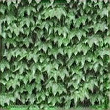
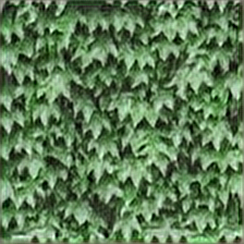
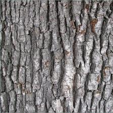
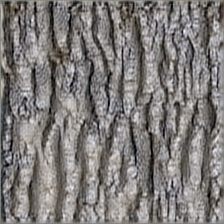
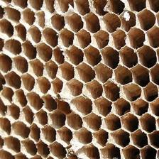
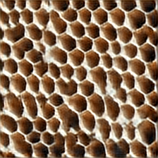
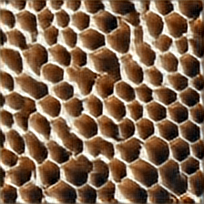
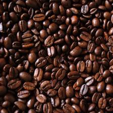
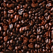
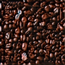
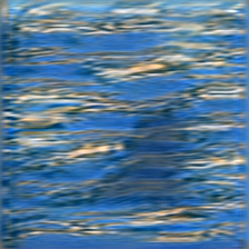
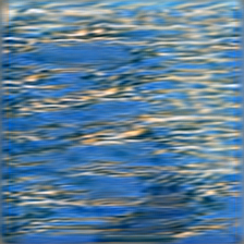
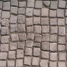
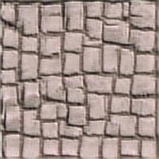
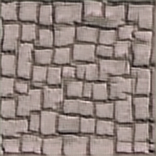
7.1 Experiment 1: Generating texture patterns
We learn a 3-layer generative ConvNet. The first layer has 100 filters with sub-sampling size of 3. The second layer has 64 filters with sub-sampling size of 1. The third layer has 30 filters with sub-sampling size of 1. We learn a generative ConvNet for each category from a single training image. Figure 1 displays the results. For each category, the first image is the training image, and the rest are 2 of the images generated by the learning algorithm.
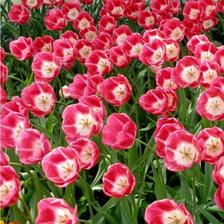
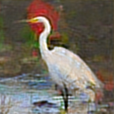
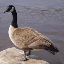
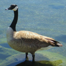
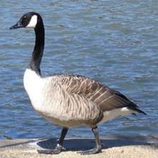
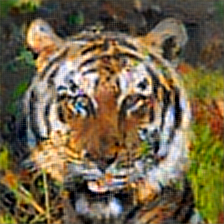
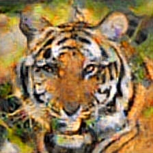
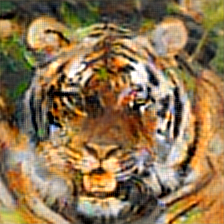
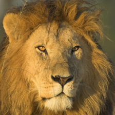
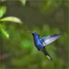
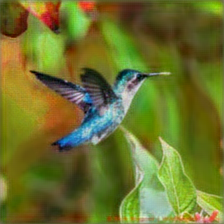
7.2 Experiment 2: Generating object patterns
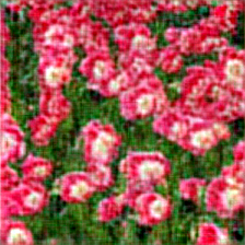
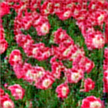
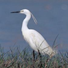
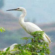
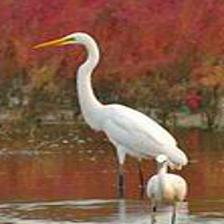
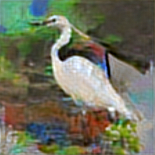
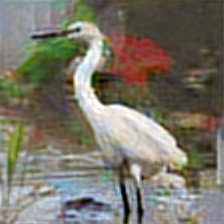
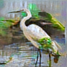
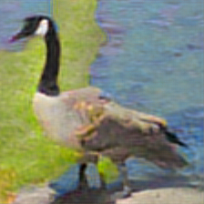
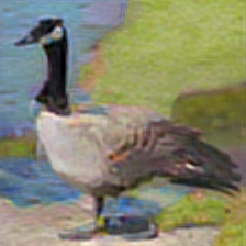
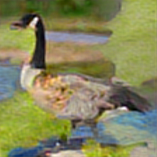
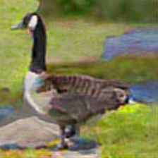
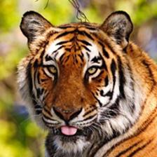
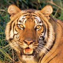
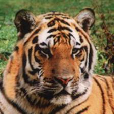
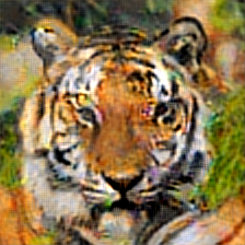
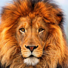
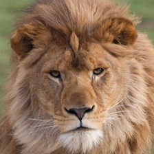
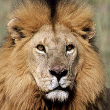
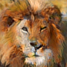
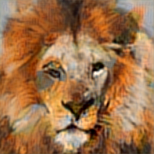
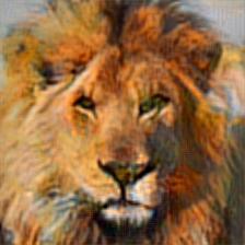
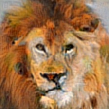
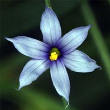
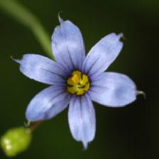
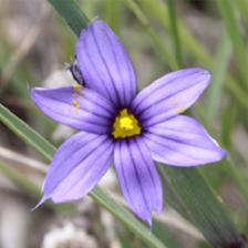
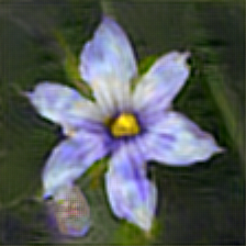
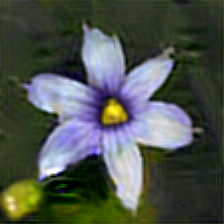
Experiment 1 shows clearly that the generative ConvNet can learn from images without alignment. We can also specialize it to learning aligned object patterns by using a single top-layer filter that covers the whole image. We learn a 4-layer generative ConvNet from images of aligned objects. The first layer has 100 filters with sub-sampling size of 2. The second layer has 64 filters with sub-sampling size of 1. The third layer has 20 filters with sub-sampling size of 1. The fourth layer is a fully connected layer with a single filter that covers the whole image. When growing the layers, we always keep the top-layer single filter, and train it together with the existing layers. We learn a generative ConvNet for each category, where the number of training images for each category is around 10, and they are collected from the Internet. Figure 2 shows the results. For each category, the first row displays 4 of the training images, and the second row shows 4 of the images generated by the learning algorithm.
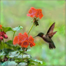
7.3 Experiment 3: Contrastive divergence learns to auto-encode
We experiment with one-step contrastive divergence learning on a small training set of 10 images collected from the Internet. The ConvNet structure is the same as in experiment 1. For computational efficiency, we learn all the layers of filters simultaneously. The number of learning iterations is . Starting from the observed images, the number of Langevin iterations is . Figure 3 shows the results. The first row displays 4 of the training images, and the second row displays the corresponding auto-encoding reconstructions with the learned parameters.
8 Conclusion
This paper derives the generative ConvNet from the discriminative ConvNet, and reveals an internal representational structure that is unique among energy-based models.
The generative ConvNet has the potential to learn from big unlabeled data, either by contrastive divergence or some reconstruction based methods.
Code and data
The code and training images can be downloaded from the project page: http://www.stat.ucla.edu/~ywu/GenerativeConvNet/main.html
Acknowledgement
The code in our work is based on the Matlab code of MatConvNet of Vedaldi & Lenc (2015). We thank the authors for making their code public.
We thank the three reviewers for their insightful comments that have helped us improve the presentation of the paper. We thank Jifeng Dai and Wenze Hu for earlier collaborations related to this work.
The work is supported by NSF DMS 1310391, ONR MURI N00014-10-1-0933 and DARPA SIMPLEX N66001-15-C-4035.
References
- Alain & Bengio (2014) Alain, Guillaume and Bengio, Yoshua. What regularized auto-encoders learn from the data-generating distribution. The Journal of Machine Learning Research, 15(1):3563–3593, 2014.
- Dai et al. (2015) Dai, Jifeng, Lu, Yang, and Wu, Ying Nian. Generative modeling of convolutional neural networks. In ICLR, 2015.
- Hinton (2002) Hinton, Geoffrey E. Training products of experts by minimizing contrastive divergence. Neural Computation, 14(8):1771–1800, 2002.
- Hinton et al. (2006a) Hinton, Geoffrey E., Osindero, Simon, and Teh, Yee-Whye. A fast learning algorithm for deep belief nets. Neural Computation, 18:1527–1554, 2006a.
- Hinton et al. (2006b) Hinton, Geoffrey E, Osindero, Simon, Welling, Max, and Teh, Yee-Whye. Unsupervised discovery of nonlinear structure using contrastive backpropagation. Cognitive Science, 30(4):725–731, 2006b.
- Hopfield (1982) Hopfield, John J. Neural networks and physical systems with emergent collective computational abilities. Proceedings of the National Academy of Sciences, 79(8):2554–2558, 1982.
- Hyvärinen (2005) Hyvärinen, Aapo. Estimation of non-normalized statistical models by score matching. Journal of Machine Learning Research, 6:695–709, 2005.
- Hyvärinen (2007) Hyvärinen, Aapo. Connections between score matching, contrastive divergence, and pseudolikelihood for continuous-valued variables. Neural Networks, IEEE Transactions on, 18(5):1529–1531, 2007.
- Krizhevsky et al. (2012) Krizhevsky, Alex, Sutskever, Ilya, and Hinton, Geoffrey E. Imagenet classification with deep convolutional neural networks. In NIPS, pp. 1097–1105, 2012.
- LeCun et al. (1998) LeCun, Yann, Bottou, Léon, Bengio, Yoshua, and Haffner, Patrick. Gradient-based learning applied to document recognition. Proceedings of the IEEE, 86(11):2278–2324, 1998.
- LeCun et al. (2006) LeCun, Yann, Chopra, Sumit, Hadsell, Rata, Ranzato, Mare’Aurelio, and Huang, Fu Jie. A tutorial on energy-based learning. In Predicting Structured Data. MIT Press, 2006.
- Lee et al. (2009) Lee, Honglak, Grosse, Roger, Ranganath, Rajesh, and Ng, Andrew Y. Convolutional deep belief networks for scalable unsupervised learning of hierarchical representations. In ICML, pp. 609–616. ACM, 2009.
- Lu et al. (2016) Lu, Yang, Zhu, Song-Chun, and Wu, Ying Nian. Learning FRAME models using CNN filters. In Thirtieth AAAI Conference on Artificial Intelligence, 2016.
- Montufar et al. (2014) Montufar, Guido F, Pascanu, Razvan, Cho, Kyunghyun, and Bengio, Yoshua. On the number of linear regions of deep neural networks. In NIPS, pp. 2924–2932, 2014.
- Ngiam et al. (2011) Ngiam, Jiquan, Chen, Zhenghao, Koh, Pang Wei, and Ng, Andrew Y. Learning deep energy models. In ICML, 2011.
- Olshausen & Field (1997) Olshausen, Bruno A and Field, David J. Sparse coding with an overcomplete basis set: A strategy employed by v1? Vision Research, 37(23):3311–3325, 1997.
- Roth & Black (2005) Roth, Stefan and Black, Michael J. Fields of experts: A framework for learning image priors. In CVPR, volume 2, pp. 860–867. IEEE, 2005.
- Salakhutdinov & Hinton (2009) Salakhutdinov, Ruslan and Hinton, Geoffrey E. Deep boltzmann machines. In AISTATS, 2009.
- Swersky et al. (2011) Swersky, Kevin, Ranzato, Marc’Aurelio, Buchman, David, Marlin, Benjamin, and Freitas, Nando. On autoencoders and score matching for energy based models. In ICML, pp. 1201–1208. ACM, 2011.
- Teh et al. (2003) Teh, Yee-Whye, Welling, Max, Osindero, Simon, and Hinton, Geoffrey E. Energy-based models for sparse overcomplete representations. The Journal of Machine Learning Research, 4:1235–1260, 2003.
- Vedaldi & Lenc (2015) Vedaldi, A. and Lenc, K. Matconvnet – convolutional neural networks for matlab. In Proceeding of the ACM Int. Conf. on Multimedia, 2015.
- Vincent (2011) Vincent, Pascal. A connection between score matching and denoising autoencoders. Neural Computation, 23(7):1661–1674, 2011.
- Wu et al. (2008) Wu, Ying Nian, Zhu, Song-Chun, and Guo, Cheng-En. From information scaling of natural images to regimes of statistical models. Quarterly of Applied Mathematics, 66:81–122, 2008.
- Xie et al. (2014) Xie, Jianwen, Hu, Wenze, Zhu, Song-Chun, and Wu, Ying Nian. Learning sparse FRAME models for natural image patterns. International Journal of Computer Vision, pp. 1–22, 2014.
- Xie et al. (2016) Xie, Jianwen, Lu, Yang, Zhu, Song-Chun, and Wu, Ying Nian. Inducing wavelets into random fields via generative boosting. Journal of Applied and Computational Harmonic Analysis, 41:4–25, 2016.
- Younes (1999) Younes, Laurent. On the convergence of markovian stochastic algorithms with rapidly decreasing ergodicity rates. Stochastics: An International Journal of Probability and Stochastic Processes, 65(3-4):177–228, 1999.
- Zeiler & Fergus (2014) Zeiler, Matthew D and Fergus, Rob. Visualizing and understanding convolutional neural networks. In ECCV, 2014.
- Zhu & Mumford (1998) Zhu, Song-Chun and Mumford, David. Grade: Gibbs reaction and diffusion equations. In ICCV, pp. 847–854, 1998.
- Zhu et al. (1997) Zhu, Song-Chun, Wu, Ying Nian, and Mumford, David. Minimax entropy principle and its application to texture modeling. Neural Computation, 9(8):1627–1660, 1997.