A Nonconforming Finite Element Method for the Biot’s Consolidation Model in Poroelasticity

Abstract

A stable finite element scheme that avoids pressure oscillations for a three-field Biot’s model in poroelasticity is considered. The involved variables are the displacements, fluid flux (Darcy velocity), and the pore pressure, and they are discretized by using the lowest possible approximation order: Crouzeix-Raviart finite elements for the displacements, lowest order Raviart-Thomas-Nédélec elements for the Darcy velocity, and piecewise constant approximation for the pressure. Mass-lumping technique is introduced for the Raviart-Thomas-Nédélec elements in order to eliminate the Darcy velocity and, therefore, reduce the computational cost. We show convergence of the discrete scheme which is implicit in time and use these types of elements in space with and without mass-lumping. Finally, numerical experiments illustrate the convergence of the method and show its effectiveness to avoid spurious pressure oscillations when mass lumping for the Raviart-Thomas-Nédélec elements is used.

1 Introduction: Biot’s Model and Three Field Formulation

Poroelasticity theory mathematically describes the interaction between the deformation of an elastic porous material and the fluid flow inside of it. A pioneer in the mathematical modeling of such coupling is Terzaghi [1] with his one-dimensional model. Later, Biot [2, 3] developed a three-dimensional mathematical model, used to date, for quantitative and qualitative study of poroelastic phenomena. Nowadays, the analysis and numerical simulation of Biot’s model become increasingly popular due to the wide range of applications in medicine, biomechanics, petroleum engineering, food processing, and other fields of science and engineering.

One of the main challenges in the numerical simulations based on the Biot’s models is the numerical instabilities in the approximation of the pressure variable (see [4, 5, 6, 7, 8]). Such instabilities occurs when materials have low permeability and/or a small time step is used at the beginning of the consolidation process. Different explanations have been provided in the literature about the nature of these instabilities. Usually, they are attributed to violation of the inf-sup condition for the Stokes problem, or the lack of monotonicity in the discrete schemes. Various numerical methods to avoid this nonphysical behavior have been analyzed. In several papers Murad, Loula, and Thomee [9, 10, 11] studied the case of stable discretizations (satisfying the inf-sup condition) for the classical two-field formulation based on displacement and pressure variables. As shown in [12, 13], however, the inf-sup condition is not a sufficient condition, and for small permeabilities the approximation to the pressure exhibits oscillations and is numerically unstable. A possible remedy is to add to the flow equation in the Biot’s model a time-dependent stabilization term, leading to oscillation free approximations of the pressure. Such stabilized discretizations, based on the MINI element [14] as well as the P1-P1 element, are proposed and analyzed in detail in [13]. Other numerical schemes, such as least squares mixed finite element methods, are proposed in [15] and [16] for a four-field formulation (displacement, stress, fluid flux and pressure). Different combinations of continuous and discontinuous Galerkin methods and mixed finite element methods for a three-field formulation are studied in [17, 18, 19]. Recently, conforming linear finite elements with stabilization for the three field problem are proposed and analyzed in [20].

Throughout this paper, we restrict our study to the quasi-static Biot’s model for soil consolidation. We assume the porous medium to be linearly elastic, homogeneous, isotropic and saturated by an incompressible Newtonian fluid. According to Biot’s theory [2], then, the consolidation process must satisfy the following system of partial differential equations:

equilibrium equation: $$-{\rm div}\,{\bm{\sigma}}^{\prime}+\alpha\nabla\,p={\bm{g}},\quad{\rm in}\,\Omega,$$ (1.1)

constitutive equation: $$\bm{\sigma}^{\prime}=2\mu\varepsilon(\bm{u})+\lambda\operatorname{div}(\bm{u}){\bm{I}},\quad{\rm in}\,\Omega,$$ (1.2)

compatibility condition: $$\varepsilon({\bm{u}})=\frac{1}{2}(\nabla{\bm{u}}+\nabla{\bm{u}}^{t}),\quad{\rm in}\,\Omega,$$ (1.3)

Darcy’s law: $${\bm{w}}=-K\nabla p,\quad{\rm in}\,\Omega,$$ (1.4)

continuity equation: $$-\alpha\ {\operatorname{div}}\,\dot{\bm{u}}-{\operatorname{div}}\,{\bm{w}}=f,\quad{\rm in}\,\Omega,$$ (1.5)

where $\lambda$ and $\mu$ are the Lamé coefficients, $\alpha$ is the Biot-Willis constant which we will assume equal to one without loss of generality, $K$ is the hydraulic conductivity, given by the quotient between the permeability of the porous medium $\kappa$ and the viscosity of the fluid $\eta$, $\bm{I}$ is the identity tensor, ${\bm{u}}$ is the displacement vector, $p$ is the pore pressure, ${\bm{\sigma}}^{\prime}$ and $\bm{\epsilon}$ are the effective stress and strain tensors for the porous medium and ${\bm{w}}$ is the percolation velocity of the fluid relative to the soil. We denote the time derivative by a dot over the letter. The right hand term ${\bm{g}}$ is the density of applied body forces and the source term $f$ represents a forced fluid extraction or injection process. Here, we consider a bounded open subset $\Omega\subset{\mathbb{R}}^{n},\;n\leq 3$ with regular boundary $\Gamma$.

This mathematical model can also be written in terms of the displacements of the solid matrix ${\bm{u}}$ and the pressure of the fluid $p$. The displacement of the structure is described by combining Hooke’s law for elastic deformation with the momentum balance equations, and the pressure of the fluid is described by combining the fluid mass conservation with Darcy’s law.

$$-\operatorname{div}\bm{\sigma}^{\prime}+\nabla p=\bm{g},\qquad\bm{\sigma}^{\prime}=2\mu\ \varepsilon(\bm{u})+\lambda\operatorname{div}(\bm{u})\bm{I},$$ (1.6)

$$-\operatorname{div}\dot{\bm{u}}+\operatorname{div}K\nabla p=f.$$ (1.7)

To complete the formulation of a well–posed problem we must add appropriate boundary and initial conditions. For instance,

$$\begin{array}[]{ccccc}p=0,&&\quad\bm{\sigma}^{\prime}\,{\bm{n}}&=&{\bm{t}},\quad\hbox{on }\Gamma_{t},\\ {\bm{u}}={\bm{0}},&&\quad\displaystyle K(\nabla p)\cdot{\bm{n}}&=&0,\quad\hbox{on }\Gamma_{c},\end{array}$$ (1.8)

where ${\bm{n}}$ is the unit outward normal to the boundary and $\Gamma_{t}\cup\Gamma_{c}=\Gamma$, with $\Gamma_{t}$ and $\Gamma_{c}$ disjoint subsets of $\Gamma$ with non null measure. For the initial time, $t=0$, the following incompressibility condition is fulfilled

$$(\nabla\cdot{\bm{u}})\,(\bm{x},0)=0,\,\bm{x}\in\Omega.$$ (1.9)

However, in many of the applications of the poroelasticity problem, the flow of the fluid through the medium is of primary interest. Although from the reduced displacement-pressure formulation the fluid flux can be recovered, a natural approach is to introduce this value as an extra primary variable instead. In this work, we are interested in this three-field formulation of the problem. The extra unknown can be seen as a disadvantage against the two-field formulation, regarding the computational cost, but there are reasons to prefer this approach. For example, the calculation of the fluid flux in post-processing is avoided in the way that the order of accuracy in its computation is higher and also the mass conservation for the fluid phase is ensured by using continuous elements for the fluid flux variable. Therefore, the governing equations of the Biot’s model, with the displacement ${\bm{u}}$, Darcy velocity ${\bm{w}}$ and pressure $p$ as primary variables are the following

$$-\operatorname{div}\bm{\sigma}^{\prime}+\nabla p=\bm{g},\qquad\bm{\sigma}^{\prime}=2\mu\varepsilon(\bm{u})+\lambda\operatorname{div}(\bm{u})\bm{I},$$ (1.10)

$${\bm{w}}+K\nabla p=0,$$ (1.11)

$$-\operatorname{div}\dot{\bm{u}}-\operatorname{div}{\bm{w}}=f.$$ (1.12)

Then, we can introduce the variational formulation for the three-field formulation of the Biot’s model as follows: Find $(\bm{u},\bm{w},p)\in\bm{V}\times\bm{W}\times Q$ such that

$$a(\bm{u},\bm{v})-(p,\operatorname{div}\bm{v})=(\bm{g},\bm{v}),\quad\forall\ \bm{v}\in\bm{V},$$ (1.13)

$$(K^{-1}\bm{w},\bm{r})-(p,\operatorname{div}\bm{r})=0,\quad\forall\ \bm{r}\in\bm{W},$$ (1.14)

$$-(\operatorname{div}\dot{\bm{u}},q)-(\operatorname{div}\bm{w},q)=(f,q),\quad\forall\ q\in Q,$$ (1.15)

where the considered functional spaces are

$${\bm{V}}=\{{\bm{u}}\in{\bm{H}}^{1}(\Omega)\ |\ {\bm{u}}|_{\Gamma_{c}}={\bm{0}}\},$$

$${\bm{W}}=\{{\bm{w}}\in\bm{H}(\operatorname{div},\Omega)\ |\ ({\bm{w}}\cdot{\bm{n}})|_{\Gamma_{c}}=0\},$$

$$Q=L^{2}(\Omega),$$

and the bilinear form $a(\bm{u},\bm{v})$ is given as the following,

$$a(\bm{u},\bm{v})=2\mu\int_{\Omega}\varepsilon(\bm{u}):\varepsilon(\bm{v})+\lambda\int_{\Omega}\operatorname{div}\bm{u}\operatorname{div}\bm{v},$$ (1.16)

which corresponds to the elasticity part, and is a continuous bilinear form. Results on well-posedness of the continuous problem were established by Showalter [21], and, for the three field formulation, Lipnikov [22]. In this work, we consider a discretization of the three-field formulation with the displacement, the Darcy velocity and the pressure as variables. More precisely, we use a nonconforming finite element space for the displacements $\bm{u}$ and conforming finite element spaces for both the Darcy velocity $\bm{w}$ and the pressure $p$. As a time stepping technique, we use the backward Euler method, and, we show that the resulting fully discrete scheme has an optimal convergence order. A similar discretization was considered in [23] for the 2D case on rectangular grids. Our scheme here works for both 2D and 3D cases on simplicial meshes and has the potential to be extended to more general meshes using the elements developed in [24] and [25]. We also show, albeit only numerically, that this nonconforming three-field scheme produces oscillation-free numerical approximations when mass-lumping is used in the Raviart-Thomas discretization for the Darcy velocity. A four-field (the stress tensor, the fluid flux, the solid displacement, and the pore pressure) discretization has also been proposed and analyzed in [26]. In [27], an improved a priori error analysis for the four-field formulation has been discussed, in which the error estimates of all the unknowns are robust for material parameters. We comment that our scheme with mass-lumping could be generalized to the four-field formulation as well.

The rest of the paper is organized as follows. In Section 2, we introduce our nonconforming spatial semi-discrete scheme. The fully discrete scheme is discussed in Section 3, where we show the well-posedness of the discrete problem and derive error estimates for the nonconforming finite element approximations. Section 4 is devoted to the numerical study of the convergence and tests the monotone behavior of the scheme and conclusions are drawn in Section 5.

2 Nonconforming Discretization

In this section, we consider spatial semi-discretization using a nonconforming finite element method. We cover $\Omega$ by simplices (triangles in 2D and tetrahedra in 3D) and have the following finite element discretization corresponding to the three-field formulation (1.13)-(1.15): Find $(\bm{u}_{h},\bm{w}_{h},p_{h})\in\bm{V}_{h}\times\bm{W}_{h}\times Q_{h}$ such that

$$a_{h}(\bm{u}_{h},\bm{v}_{h})-(p_{h},\operatorname{div}\bm{v}_{h})=(\bm{g}(t),\bm{v}_{h}),\quad\forall\ \bm{v}_{h}\in\bm{V}_{h},$$ (2.1)

$$(K^{-1}\bm{w}_{h},\bm{r}_{h})_{h}-(p_{h},\operatorname{div}\bm{r}_{h})=0,\quad\forall\ \bm{r}_{h}\in\bm{W}_{h}$$ (2.2)

$$-(\operatorname{div}\dot{\bm{u}}_{h},q_{h})-(\operatorname{div}\bm{w}_{h},q_{h})=(f(t),q_{h}),\quad\forall\ q_{h}\in Q_{h}.$$ (2.3)

Here, $\bm{V}_{h}$ is the Crouzeix-Raviart finite element space [28], $\bm{W}_{h}$ the lowest order Raviart-Thomas-Nédélec space [29, 30, 31], and $Q_{h}$ is the space of piecewise constant functions (with respect to the triangulation $\mathcal{T}_{h}$). Further details are discussed later in this section.

2.1 Interfaces, Normal Vectors and Jumps of Traces of Functions

Let us first introduce some notation. We denote the set of faces (interfaces) in the triangulation $\mathcal{T}_{h}$ by $\mathcal{E}$ and introduce the set of boundary faces $\mathcal{E}^{\partial}$, and the set of interior faces $\mathcal{E}^{o}$. We have $\mathcal{E}=\mathcal{E}^{o}\cup\mathcal{E}^{\partial}$.

Let us fix $e\in\mathcal{E}^{o}$ and let $T\in\mathcal{T}_{h}$ be such that $e\in\partial T$. We set $\bm{n}_{e,T}$ to be the unit outward (with respect to $T$) normal vector to $e$. In addition, with every face $e\in\mathcal{E}^{o}$, we also associate a unit vector $\bm{n}_{e}$ which is orthogonal to the $(d-1)$ dimensional affine variety (line in 2D and plane in 3D) containing the face. For the boundary faces, we always set $\bm{n}_{e}=\bm{n}_{e,T}$, where $T$ is the unique element for which we have $e\in\partial T$. In our setting, for the interior faces, the particular direction of $\bm{n}_{e}$ does not really matter, although it is important that this direction is fixed for every face. Thus, for $e\in\mathcal{E}$, we define $T^{+}(e)$ and $T^{-}(e)$ as follows:

$$T^{\pm}(e):=\{T\in\mathcal{T}_{h}\ \mbox{such that}\ e\in\partial T,\ \mbox{and}\ (\bm{n}_{e}\cdot\bm{n}_{e,T})=\pm 1\}.$$

It is immediate to see that both sets defined above contain no more than one element, that is: for every face we have exactly one $T^{+}(e)$ and for the interior faces we also have exactly one $T^{-}(e)$. For the boundary faces we only have $T^{+}(e)$. In the following, we write $T^{\pm}$ instead of $T^{\pm}(e)$, when this does not cause confusion and ambiguity.

Next, for a given function $u$ (vector or scalar valued) its jump across an interior face $e\in\mathcal{E}^{o}$ is denoted by $[\![u]\!]_{e}$, and defined as

$$[\![u]\!]_{e}(x)=u_{T^{+}(e)}(x)-u_{T^{-}(e)}(x),\quad x\in e.$$

2.2 Finite Element Spaces

We now give the definitions of the finite element spaces used in the semi-discretization (2.1)–(2.3).

2.2.1 Nonconforming Crouzeix-Raviart Space

The Crouzeix-Raviart space $\bm{V}_{h}$ consists of vector valued functions which are linear on every element $T\in\mathcal{T}_{h}$ and satisfy the following continuity conditions

$$\bm{V}_{h}=\left\{\bm{v}_{h}\in{\bm{L}}^{2}(\Omega)\;\bigg{|}\int_{e}[\![\bm{v}_{h}]\!]_{e}=0,\;\;\mbox{for all}\;e\in\mathcal{E}^{o}\right\}.$$

Equivalently, all functions from $\bm{V}_{h}$ are continuous at the barycenters of the faces in $\mathcal{E}^{o}$. For the boundary faces, the elements of $\bm{V}_{h}$ are zero in the barycenters of any face on the Dirichlet boundary.

2.2.2 Raviart-Thomas-Nédélec Space

We now consider the standard lowest order Raviart-Thomas-Nédélec space $\bm{W}_{h}$. Recall that every element $\bm{v}_{h}\in\bm{W}_{h}$ can be written as

$$\bm{v}_{h}=\sum_{e\in\mathcal{E}_{h}}e(\bm{v}_{h})\bm{\psi}_{e}(\bm{x}),$$ (2.4)

Here, $e(\cdot)$ denotes the functional (as known as the degree of freedom) associated with the face $e\in\mathcal{E}$ and its action on a function $\bm{v}$ for which $\bm{v}\cdot\bm{n}_{e}$ is in $L^{2}(e)$ is defined as

$$e(\bm{v})=\int_{e}\bm{v}\cdot\bm{n}_{e}.$$

To define $\bm{W}_{h}$, we only need to define the basis functions $\bm{\psi}_{e}$, for $e\in\mathcal{E}$, dual to the degrees of freedom $e(\cdot)$. If $e$ is the face opposite to the vertex $P_{e}$ of the triangle/tetrahedron $T$, then

$$\bm{\psi}_{e}\big{|}_{T}=\frac{(\bm{n}_{e}\cdot\bm{n}_{e,T})}{d|T|}(\bm{x}-\bm{x}_{P_{e}})=\pm\frac{1}{d|T|}(\bm{x}-\bm{x}_{P_{e}}).$$ (2.5)

We note that explicit formulae similar to (2.5) are available also for the case of lowest order Raviart-Thomas-Nédélec elements on $d$-dimensional rectangular elements (parallelograms or rectangular parallelepipeds). For any such element $T\in\mathcal{T}_{h}$ with faces parallel to the coordinate planes (axes) let $\bm{\psi}_{k}^{\pm}$ denote the basis function corresponding to the functional $F_{k}^{\pm}(\cdot)$. Clearly, the outward normal vectors to the faces of such an element are the $\pm\bm{e}_{k}$, $k=1,\ldots,d$, where $\bm{e}_{k}$ is the $k$-th coordinate vector in $\mathbb{R}^{d}$. Let $\bm{x}_{M,k}^{\pm}\in\mathbb{R}^{d}$ be the mass center of the face $F_{k}^{\pm}$, $k=1,\ldots,d$. We then have

$$\bm{\psi}_{k}^{\pm}(\bm{x})=\frac{(\bm{x}-\bm{x}_{M,k}^{\mp})^{T}\bm{e}_{k}}{|T|}\bm{e}_{k}.$$ (2.6)

From this formula we see that over the finite element $T$ the basis functions $\bm{\psi}_{k}^{\pm}(\bm{x})$ are linear in $\bm{x}_{k}$ and constant in the remaining variables in $\mathbb{R}^{d}$.

2.2.3 Piecewise Constant Space

For approximating the pressure, we use the piecewise constant space spanned by the characteristic functions of the elements, i.e. $Q_{h}=\operatorname{span}\{\chi_{T}\}_{T\in\mathcal{T}_{h}}$.

2.3 Approximate Variational Formulation

We first consider the bilinear form $a_{h}(\cdot,\cdot):\bm{V}_{h}\times\bm{V}_{h}\mapsto\mathbb{R}$. Before we write out the details, we have to assume that $\Gamma_{c}$ is non-empty. If $\Gamma_{c}=\emptyset$, i.e., $\Gamma_{t}=\Gamma$ (the pure traction problem), $a(\cdot,\cdot)$ is a positive semidefinite form and the dimension of its null space equals the number of edges on the boundary (for both 2D and 3D). Therefore, the Korn’s inequality fails. Even if $\Gamma_{c}\neq\emptyset$, for some cases, Korn’s inequality may fail for the standard discretization by Crouzeix-Raviart elements without additional stabilization. In summary, if we simply take $a_{h}(\cdot,\cdot)=a(\cdot,\cdot)$ then it does not satisfy the discrete Korn inequality and, therefore, $a_{h}(\cdot,\cdot)$ is not coercive. Moreover, it is also possible that Korn’s inequality hold, but the constant will approach infinity as the mesh size $h$ approaches zero. In another words, if we use $a_{h}(\cdot,\cdot)=a(\cdot,\cdot)$, the coercivity constant blows up when $h$ approaches zero. For discussions on nonconforming linear elements for elasticity problems and discrete Korn’s inequality, we refer to [32, 33] for more details.

One way to fix the potential problem is to add stabilization. The following perturbation of the bilinear form which does satisfy the Korn’s inequality was proposed by Hansbo and Larson [34].

$$a_{h}(\bm{v},\bm{w})=a(\bm{v},\bm{w})+a_{\textrm{\tiny J}}(\bm{v},\bm{w}),\quad\mbox{where}\quad a_{\textrm{\tiny J}}(\bm{v},\bm{w})=2\mu\gamma_{1}\sum_{e\in\mathcal{E}}h_{e}^{-1}\int_{e}[\![\bm{v}]\!]_{e}[\![\bm{w}]\!]_{e}.$$

Here, the constant $\gamma_{1}>0$ is a fixed real number away from $0$ (i.e. $\gamma_{1}=\frac{1}{2}$ is an acceptable choice). As shown in Hansbo and Larson [34] the bilinear form $a_{h}(\cdot,\cdot)$ is positive definite and the corresponding error is of optimal (first) order in the corresponding energy norm. Moreover, the resulting method is locking free and we use such $a_{h}(\cdot,\cdot)$ in our nonconforming scheme.

Remark 1

In [34], the jump term $a_{\textrm{\tiny J}}(\cdot,\cdot)$ includes all the edges, i.e., the stabilization needs to be done on both interior and boundary edges. In [35], it has been shown that the jump stabilization only needs to be added to the interior edges and boundary edges with Neumann boundary conditions and the discrete Korn’s inequality still holds. In fact, in [36], it is suggested that only the normal component of the jumps on the edges is needed for the stabilization in order to satisfy the discrete Korn’s equality.

We next consider the bilinear form in (2.2), denoted by $(\cdot,\cdot)_{h}$. The first choice for such a form is just taking the usual $L^{2}(\Omega)$ inner product, i.e. $(\bm{w},\bm{r})_{h}=(\bm{w},\bm{r})=\int_{\Omega}\bm{w}\cdot\bm{r}$. This is a standard choice and leads to a mass matrix in the Raviart-Thomas-Nédélec element when we write out the matrix form.

The second choice, which is the bilinear form we use here, is based on mass lumping in the Raviart-Thomas space, i.e.,

$$(\bm{r},\bm{s})_{h}=\sum_{T}\sum_{e\subset\partial T}\omega_{e}\ e(\bm{r})e(\bm{s}).$$ (2.7)

We refer to [37] and [38] for details on determining the weights $\omega_{e}$, which are $\omega_{e}=\displaystyle\frac{|e|d_{e}}{d}$ with $d_{e}$ being the signed distance between the Voronoi vertices adjacent to the face $e$. Such weights, in the two-dimensional case, are chosen so that

$$(\bm{w},\bm{r})_{h}=\int_{\Omega}\bm{w}\cdot\bm{r},\quad\bm{w},\bm{r}\in\bm{W}_{h}\ \text{and}\ \bm{w},\bm{r}\ \text{are piecewise constants},$$ (2.8)

which implies the equivalence between $(\bm{w},\bm{r})_{h}$ and the standard $L^{2}$ inner product $(\bm{w},\bm{r})$. The situation in 3D is a little bit involved since (2.8) in general does not hold. Nevertheless, in [37], it has been shown that the mixed formulation for Poisson equation using the mass-lumping maintains the optimal convergence order, which is what we need for the convergence analysis of our scheme later in Section 3.

Remark 2

As shown in [37], the mass-lumping technique is quite general and works for both two- and three-dimensional cases. For the convergence analysis of the mass-lumping, they assume that the circumcenters are inside the simplex. Such partition exists in general (see [39]). Moreover, they also pointed out that this assumption is not strictly necessary and can be relaxed. When the mesh contains pairs of right triangles in 2D and right tetrahedrons in 3D, $d_{e}$ degenerates to zero and so is the weight $\omega_{e}$. However, we can remedy by combining the pressure unknowns on these pairs to just one pressure unknown.

In practice, such lumped mass approximation results in a block diagonal matrix and, therefore, we can eliminate the Darcy velocity $\bm{w}$ and reduce the three-field formulation to two-field formulation involving only displacement $\bm{u}$ and pressure $p$. In practice, such elimination reduces the size of the linear system that needs to be solved at each time step and save computational cost. In the literature, there have been other similar techniques for eliminating the Darcy velocity $\bm{w}$. For example, numerical integration [40] and multipoint flux mixed formulation [41]. In addition, for Biot’s model, as shown by numerical experiments in Section 4, the lumped mass approximation actually gives an oscillation-free approximation while maintains the optimal error estimates.

3 Analysis of the Fully Discrete Scheme

In this section, we consider the fully discrete scheme of (1.13)–(1.15) at time $t_{n}=n\tau$, $n=1,2,\ldots$ as following: Find $(\bm{u}_{h}^{n},\bm{w}_{h}^{n},p_{h}^{n})\in\bm{V}_{h}\times\bm{W}_{h}\times Q_{h}$ such that

$$a_{h}(\bm{u}_{h}^{n},\bm{v}_{h})-(p_{h}^{n},\operatorname{div}\bm{v}_{h})=(\bm{g}(t_{n}),\bm{v}_{h}),\quad\forall\ \bm{v}_{h}\in\bm{V}_{h},$$ (3.1)

$$(K^{-1}\bm{w}_{h}^{n},\bm{r}_{h})_{h}-(p_{h}^{n},\operatorname{div}\bm{r}_{h})=0,\quad\forall\ \bm{r}_{h}\ \in\bm{W}_{h}$$ (3.2)

$$-(\operatorname{div}\bar{\partial}_{t}\bm{u}_{h}^{n},q_{h})-(\operatorname{div}\bm{w}_{h}^{n},q_{h})=(f(t_{n}),q_{h}),\quad\forall\ q_{h}\in Q_{h},$$ (3.3)

where $\tau$ is the time step size and $\bar{\partial}_{t}\bm{u}_{h}^{n}:=(\bm{u}_{h}^{n}-\bm{u}_{h}^{n-1})/\tau$. For the initial data $\bm{u}_{h}^{0}$, we use the discrete counterpart of (1.9), i.e.,

$$\operatorname{div}\bm{u}_{h}^{0}=0.$$ (3.4)

We will first consider the well-posedness of the linear system (3.1)-(3.3) at each time step $t_{n}$ and then derive the error estimates for the fully discrete scheme.

3.1 Well-posedness

We consider the following linear system derived from (3.1)-(3.3): Find $(\bm{u}_{h},\bm{w}_{h},p_{h})\in\bm{V}_{h}\times\bm{W}_{h}\times Q_{h}$ such that

$$a_{h}(\bm{u}_{h},\bm{v}_{h})-(p_{h},\operatorname{div}\bm{v}_{h})=(\bm{g},\bm{v}_{h}),\quad\forall\ \bm{v}_{h}\in\bm{V}_{h},$$ (3.5)

$$\tau(K^{-1}\bm{w}_{h},\bm{r}_{h})_{h}-\tau(p_{h},\operatorname{div}\bm{r}_{h})=0,\quad\forall\ \bm{r}_{h}\ \in\bm{W}_{h}$$ (3.6)

$$-(\operatorname{div}\bm{u}_{h},q_{h})-\tau(\operatorname{div}\bm{w}_{h},q_{h})=(\tilde{f},q_{h}),\quad\forall\ q_{h}\in Q_{h},$$ (3.7)

Here, to simplify the presentation, we have omitted the superscript $n$ because the results are independent of the time step. We have denoted $\tilde{f}:=\tau f(t_{n})-\operatorname{div}\bm{u}_{h}^{n-1}$, and we note that the relations (3.6) and (3.7) are obtained by multiplying (3.2) and (3.3) with the time step size $\tau$.

We equip the space $\bm{V}\times\bm{W}\times Q$ with the following norm

$$\|(\bm{u},\bm{w},p)\|_{\tau}:=\left(\|\bm{u}\|^{2}_{1}+\tau\|\bm{w}\|^{2}+\tau^{2}\|\operatorname{div}\bm{w}\|^{2}+\|p\|^{2}\right)^{1/2},$$ (3.8)

where $\|\cdot\|_{1}$ and $\|\cdot\|$ denote the standard $H^{1}$ norm and $L^{2}$ norm, respectively. In the analysis we need the following composite bilinear form (including all variables):

$$B(\bm{u}_{h},\bm{w}_{h},p_{h};\bm{v}_{h},\bm{r}_{h},q_{h}) :=a_{h}(\bm{u}_{h},\bm{v}_{h})-(p_{h},\operatorname{div}\bm{v}_{h})+\tau(K^{-1}\bm{w}_{h},\bm{r}_{h})_{h}$$

$$\quad-\tau(p_{h},\operatorname{div}\bm{r}_{h})-(\operatorname{div}\bm{u}_{h},q_{h})-\tau(\operatorname{div}\bm{w}_{h},q_{h}).$$

Note that

$$\operatorname{div}\bm{W}_{h}\subseteq Q_{h}.$$ (3.9)

Further, we note the following continuity, coercivity and stability (inf-sup) conditions on the bilinear forms involved in the definition of $B(\cdot,\cdot,\cdot;\cdot,\cdot,\cdot)$:

$$a_{h}(\bm{u}_{h},\bm{v}_{h})\leq C_{\bm{V}}\|\bm{u}_{h}\|_{1}\|\bm{v}_{h}\|_{1},\quad\forall\ \bm{u}_{h},\bm{v}_{h}\in\bm{V}_{h},$$ (3.10)

$$a_{h}(\bm{u}_{h},\bm{u}_{h})\geq\alpha_{\bm{V}}\|\bm{u}_{h}\|_{1}^{2},\quad\forall\ \bm{u}_{h}\in\bm{V}_{h},$$ (3.11)

$$c_{K}\|\bm{w}_{h}\|^{2}\leq(K^{-1}\bm{w}_{h},\bm{w}_{h})_{h}\leq C_{K}\|\bm{w}_{h}\|^{2},\quad\forall\ \bm{w}_{h}\in\bm{W}_{h},$$ (3.12)

$$\inf_{p_{h}\in Q_{h}}\sup_{\bm{u}_{h}\in\bm{V}_{h}}\frac{(\operatorname{div}\bm{u}_{h},p_{h})}{\|\bm{u}_{h}\|_{1}\|p_{h}\|}=\beta_{\bm{V}}>0.$$ (3.13)

Under these conditions, which are satisfied by our choice of finite element spaces and discrete bilinear forms, we have the following theorem showing the solvability of the linear system (3.5)-(3.7).

Theorem 1

If the conditions (3.9)-(3.13) hold, then the bilinear form $B(\cdot,\cdot,\cdot;\cdot,\cdot,\cdot)$ satisfies the following inf-sup condition,

$$\sup_{(\bm{v}_{h},\bm{r}_{h},q_{h})\in\bm{V}_{h}\times\bm{W}_{h}\times Q_{h}}\frac{B(\bm{u}_{h},\bm{w}_{h},p_{h};\bm{v}_{h},\bm{r}_{h},q_{h})}{\|\left(\bm{v}_{h},\bm{r}_{h},q_{h}\right)\|_{\tau}}\geq\gamma\|\left(\bm{u}_{h},\bm{w}_{h},p_{h}\right)\|_{\tau}$$ (3.14)

with a constant $\gamma>0$ independent of mesh size $h$ and time step size $\tau$. Moreover, the three field formulation (3.5)-(3.7) is well-posed.

Proof

According to the inf-sup condition (3.13), we have for $p_{h}$, there exists $\bm{h}_{h}\in\bm{V}_{h}$, such that

$$(\operatorname{div}\bm{h}_{h},p_{h})\geq\beta_{\bm{V}}\|p_{h}\|^{2},\quad\|p_{h}\|=\|\bm{h}_{h}\|_{1}.$$ (3.15)

Note that, according to the condition (3.9), $\operatorname{div}\bm{w}_{h}\in Q_{h}$. Let $\bm{v}_{h}=\bm{u}_{h}-\theta_{1}\bm{h}_{h}$, $\bm{r}_{h}=\bm{w}_{h}$, $q_{h}=-(p_{h}+\theta_{2}\tau\operatorname{div}\bm{w}_{h})$, then we have,

$$B(\bm{u}_{h},\bm{w}_{h},p_{h};\bm{v}_{h},\bm{r}_{h},q_{h}) =a_{h}(\bm{u}_{h},\bm{u}_{h}-\theta_{1}\bm{h}_{h})-(p_{h},\operatorname{div}(\bm{u}_{h}-\theta_{1}\bm{h}_{h}))+\tau(K^{-1}\bm{w}_{h},\bm{w}_{h})_{h}-\tau(p_{h},\operatorname{div}\bm{w}_{h})$$

$$\quad\ -(\operatorname{div}\bm{u}_{h},-p_{h}-\theta_{2}\tau\operatorname{div}\bm{w}_{h})-\tau(\operatorname{div}\bm{w}_{h},-p_{h}-\theta_{2}\tau\operatorname{div}\bm{w}_{h})$$

$$=\|\bm{u}_{h}\|_{a_{h}}^{2}-\theta_{1}a_{h}(\bm{u}_{h},\bm{h}_{h})+\theta_{1}(p_{h},\operatorname{div}\bm{h}_{h})+\tau(K^{-1}\bm{w}_{h},\bm{w}_{h})_{h}$$

$$\quad+\theta_{2}(\operatorname{div}\bm{u}_{h},\tau\operatorname{div}\bm{w}_{h})+\theta_{2}\tau^{2}\|\operatorname{div}\bm{w}_{h}\|^{2}$$

$$\geq\|\bm{u}_{h}\|_{a_{h}}^{2}-\frac{\theta_{1}\epsilon_{1}}{2}\|\bm{u}_{h}\|_{a_{h}}^{2}-\frac{\theta_{1}}{2\epsilon_{1}}\|\bm{h}_{h}\|_{a_{h}}^{2}+\theta_{1}\beta_{\bm{V}}\|p_{h}\|^{2}+c_{K}\,\tau\|\bm{w}_{h}\|^{2}$$

$$\quad-\frac{\theta_{2}\epsilon_{2}}{2}\|\operatorname{div}\bm{u}_{h}\|^{2}-\frac{\theta_{2}}{2\epsilon_{2}}\tau^{2}\|\operatorname{div}\bm{w}_{h}\|^{2}+\theta_{2}\tau^{2}\|\operatorname{div}\bm{w}_{h}\|^{2}$$

$$\geq\left(1-\frac{\theta_{1}\epsilon_{1}}{2}\right)\|\bm{u}_{h}\|_{a_{h}}^{2}-\frac{\theta_{1}C_{\bm{V}}}{2\epsilon_{1}}\|p_{h}\|^{2}+\theta_{1}\beta_{\bm{V}}\|p_{h}\|^{2}+c_{K}\,\tau\|\bm{w}_{h}\|^{2}$$

$$\quad-\theta_{2}\epsilon_{2}\|\bm{u}_{h}\|_{1}^{2}-\frac{\theta_{2}}{2\epsilon_{2}}\tau^{2}\|\operatorname{div}\bm{w}_{h}\|^{2}+\theta_{2}\tau^{2}\|\operatorname{div}\bm{w}_{h}\|^{2}$$

$$\geq\left[\alpha_{\bm{V}}\left(1-\frac{\theta_{1}\epsilon_{1}}{2}\right)-\theta_{2}\epsilon_{2}\right]\|\bm{u}_{h}\|_{1}^{2}+c_{K}\,\tau\|\bm{w}_{h}\|^{2}$$

$$\quad+\theta_{2}\left(1-\frac{1}{2\epsilon_{2}}\right)\tau^{2}\|\operatorname{div}\bm{w}_{h}\|^{2}+\left[\theta_{1}\left(\beta_{\bm{V}}-\frac{C_{\bm{V}}}{2\epsilon_{1}}\right)\right]\|p_{h}\|^{2}.$$

Choose $\theta_{1}=\frac{\beta_{\bm{V}}}{C_{\bm{V}}}$, $\epsilon_{1}=\frac{C_{\bm{V}}}{\beta_{\bm{V}}}$, $\theta_{2}=\frac{\alpha_{\bm{V}}}{3}$, and $\epsilon_{2}=1$, we have

$$B(\bm{u}_{h},\bm{w}_{h},p_{h};\bm{v}_{h},\bm{r}_{h},q_{h}) \geq\frac{\alpha_{\bm{V}}}{6}\|\bm{u}_{h}\|_{1}^{2}+c_{K}\,\tau\|\bm{w}_{h}\|^{2}+\frac{\alpha_{\bm{V}}}{6}\tau^{2}\|\operatorname{div}\bm{w}_{h}\|^{2}+\frac{\beta_{\bm{V}}^{2}}{2C_{\bm{V}}}\|p_{h}\|^{2}$$

$$\geq C_{1}\|\left(\bm{u}_{h},\bm{w}_{h},p_{h}\right)\|_{\tau}^{2},$$

where $\displaystyle C_{1}=\min\left\{\frac{\alpha_{\bm{V}}}{6},c_{K},\frac{\beta_{\bm{V}}^{2}}{2C_{\bm{V}}}\right\}$.

On the other hand, we have

$$\|\left(\bm{v}_{h},\bm{r}_{h},q_{h}\right)\|_{\tau}^{2} =\|\bm{u}_{h}-\theta_{1}\bm{h}_{h}\|_{1}^{2}+\tau\|\bm{w}_{h}\|^{2}+\tau^{2}\|\operatorname{div}\bm{w}_{h}\|^{2}+\|-p_{h}-\theta_{2}\tau\operatorname{div}\bm{w}_{h}\|^{2}$$

$$\leq 2\|\bm{u}_{h}\|_{1}^{2}+2\theta_{1}^{2}\|\bm{h}_{h}\|_{1}^{2}+\tau\|\bm{w}_{h}\|^{2}+\tau^{2}\|\operatorname{div}\bm{w}_{h}\|^{2}+2\|p_{h}\|^{2}+2\theta_{2}^{2}\tau^{2}\|\operatorname{div}\bm{w}_{h}\|^{2}$$

$$=2\|\bm{u}_{h}\|_{1}^{2}+\tau\|\bm{w}_{h}\|^{2}+\left(1+\frac{2\alpha_{\bm{V}}^{2}}{9}\right)\tau^{2}\|\operatorname{div}\bm{w}_{h}\|^{2}+\left(2\frac{\beta_{\bm{V}}^{2}}{C_{\bm{V}}^{2}}+2\right)\|p_{h}\|^{2}$$

$$\leq C_{2}\|\left(\bm{u}_{h},\bm{w}_{h},p_{h}\right)\|_{\tau}^{2},$$

where $\displaystyle C_{2}:=\max\left\{2,1+\frac{2\alpha^{2}_{\bm{V}}}{9},2\frac{\beta_{\bm{V}}^{2}}{C_{\bm{V}}^{2}}+2\right\}$. Then (3.14) follows with $\gamma:=C_{1}C_{2}^{\frac{1}{2}}$.

Moreover, it is easy to show that the bilinear form $B(\bm{u}_{h},\bm{w}_{h},p_{h};\bm{v}_{h},\bm{r}_{h},q_{h})$ is continuous, therefore, we can conclude that the three-field formulation is well-posed.      

Remark 3

The continuity condition (3.10) follows from the definition of bilinear form and the corresponding norms. The coercivity condition (3.11) follows from discrete Korn’s equality, which hinges on the stabilization provided by the jump-jump term $a_{\textrm{\tiny J}}(\cdot,\cdot)$. We refer to [34] for details on this. The condition (3.12) follows from the property of the lumped mass procedure and we refer to [37] for details. The last condition (3.13) is the standard inf-sup condition for the nonconforming finite element methods for solving the Stokes equation, see [28] for details.

3.2 Error Estimates

To derive the error analysis of the fully discrete scheme (3.1)-(3.3), following the standard error analysis of time-dependent problems in Thomée [42], we first define the following elliptic projections $\bar{\bm{u}}_{h}\in\bm{V}_{h}$, $\bar{\bm{w}}_{h}\in\bm{W}_{h}$, and $\bar{p}_{h}\in Q_{h}$ for $t>0$ as usual,

$$a_{h}(\bar{\bm{u}}_{h},\bm{v}_{h})-(\bar{p}_{h},\operatorname{div}\bm{v}_{h})=a_{h}(\bm{u},\bm{v}_{h})-(p,\operatorname{div}\bm{v}_{h}),\quad\forall\bm{v}_{h}\in\bm{V}_{h},$$ (3.16)

$$(K^{-1}\bar{\bm{w}}_{h},\bm{r}_{h})_{h}-(\bar{p}_{h},\operatorname{div}\bm{r}_{h})=(K^{-1}\bm{w},\bm{r}_{h})-(p,\operatorname{div}\bm{r}_{h}),\quad\forall\bm{r}_{h}\in\bm{W}_{h},$$ (3.17)

$$(\operatorname{div}\bar{\bm{w}}_{h},q_{h})=(\operatorname{div}\bm{w},q_{h}),\quad\forall q_{h}\in Q_{h}.$$ (3.18)

Note that the above elliptic projections are actually decoupled; $\bar{\bm{w}}_{h}$ and $\bar{p}_{h}$ are defined by (3.17) and (3.18) which is the mixed formulation of the Poisson equation. Therefore, the existence and uniqueness of $\bar{\bm{w}}_{h}$ and $\bar{p}_{h}$ follow directly from the standard results of mixed formulation of the Poisson equation (for the mass-lumping case, we refer to [37] for details). After $\bar{p}_{h}$ is defined, $\bar{\bm{u}}_{h}$ can be determined by solving (3.16) which is a linear elasticity problem, and the existence and uniqueness of $\bar{\bm{u}}_{h}$ also follow from the standard results of the linear elasticity problem. Now we can split the errors as follows

$$\bm{u}(t_{n})-\bm{u}_{h}^{n}=\left(\bm{u}(t_{n})-\bar{\bm{u}}_{h}(t_{n})\right)-\left(\bm{u}_{h}^{n}-\bar{\bm{u}}_{h}(t_{n})\right)=:\rho_{\bm{u}}^{n}-e_{\bm{u}}^{n},$$

$$\bm{w}(t_{n})-\bm{w}_{h}^{n}=\left(\bm{w}(t_{n})-\bar{\bm{w}}_{h}(t_{n})\right)-\left(\bm{w}_{h}^{n}-\bar{\bm{w}}_{h}(t_{n})\right)=:\rho_{\bm{w}}^{n}-e_{\bm{w}}^{n},$$

$$p(t_{n})-p_{h}^{n}=\left(p(t_{n})-\bar{p}_{h}(t_{n})\right)-\left(p_{h}^{n}-\bar{p}_{h}(t_{n})\right)=:\rho_{p}^{n}-e_{p}^{n}.$$

For the errors for the elliptic projections, we have, for $t>0$,

$$\|\rho_{\bm{u}}\|_{a_{h}}\leq ch\left(\|\bm{u}\|_{2}+\|p\|_{1}\right),$$ (3.19)

$$\|\rho_{\bm{w}}\|\leq ch\|\bm{w}\|_{1},$$ (3.20)

$$\|\rho_{p}\|\leq ch\left(\|p\|_{1}+\|\bm{w}\|_{1}\right).$$ (3.21)

Note that (3.19) follows from the standard error analysis of linear elasticity problems. (3.20) and (3.21) follow from the error analysis of the mixed formulation of Poisson problems. If the mass-lumping is applied, such error analysis can be found in [37].

We can similarly define the elliptic projection $\overline{\partial_{t}\bm{u}}$, $\overline{\partial_{t}\bm{w}}$, and $\overline{\partial_{t}p}$ of $\partial_{t}\bm{u}$, $\partial_{t}\bm{w}$, and $\partial_{t}p$ respectively. And we have the estimates above also for $\partial_{t}\rho_{\bm{u}}$, $\partial_{t}\rho_{\bm{w}}$, and $\partial_{t}\rho_{p}$ as well, where on the right hand side of the inequalities we have the norms of $\partial_{t}\bm{u}$, $\partial_{t}\bm{w}$, and $\partial_{t}p$ instead of the norms of $\bm{u}$, $\bm{w}$, and $p$ respectively.

We define the following norm on the finite element spaces:

$$\|(\bm{u},\bm{w},p)\|_{\tau,h}:=\left(\|\bm{u}\|_{a_{h}}^{2}+\tau\|\bm{w}\|_{K^{-1},h}^{2}+\|p\|^{2}\right)^{1/2},$$

where $\|\bm{w}\|_{K^{-1},h}^{2}:=(K^{-1}\bm{w},\bm{w})_{h}$.

Now we need to estimate the errors $e_{\bm{u}}$, $e_{\bm{w}}$, and $e_{p}$, and then the overall error estimates can be derived by the triangular inequality. Next lemma gives the error estimates of $e_{\bm{u}}$, $e_{\bm{w}}$, and $e_{p}$.

Lemma 2

Let $R_{\bm{u}}^{j}:=\partial_{t}\bm{u}(t_{j})-\frac{\bar{\bm{u}}_{h}(t_{j})-\bar{\bm{u}}_{h}(t_{j-1})}{\tau}$, we have

$$\|(e_{\bm{u}}^{n},e_{\bm{w}}^{n},e_{p}^{n})\|_{\tau,h}\leq c\left(\|e_{\bm{u}}^{0}\|_{a_{h}}+\tau\sum_{j=1}^{n}\|R_{\bm{u}}^{j}\|_{a_{h}}\right)$$ (3.22)

Proof

Choosing $\bm{v}=\bm{v}_{h}$ in (1.13), $\bm{r}=\bm{r}_{h}$ in (1.14), and $q=q_{h}$ in (1.15), and subtracting these three equations from (3.1), (3.2), and (3.3), we have

$$a_{h}(e_{\bm{u}}^{n},\bm{v}_{h})-(e_{p}^{n},\operatorname{div}\bm{v}_{h})=0,$$ (3.23)

$$(K^{-1}e_{\bm{w}}^{n},\bm{r}_{h})_{h}-(e_{p}^{n},\operatorname{div}\bm{r}_{h})=0,$$ (3.24)

$$-(\operatorname{div}\bar{\partial}_{t}e_{\bm{u}}^{n},q_{h})-(\operatorname{div}e_{\bm{w}}^{n},q_{h})=-(\operatorname{div}R_{\bm{u}}^{n},q_{h}).$$ (3.25)

Choosing $\bm{v}_{h}=\bar{\partial}_{t}e_{\bm{u}}^{n}$, $\bm{r}_{h}=e_{\bm{w}}^{n}$ and $q_{h}=-e_{p}^{n}$ in (3.23), (3.24), and (3.25), respectively, and adding them, we have

$$\|e_{\bm{u}}^{n}\|_{a_{h}}^{2}+\tau\|e_{\bm{w}}^{n}\|_{K^{-1},h}^{2} =a_{h}(e_{\bm{u}}^{n},e_{\bm{u}}^{n-1})+\tau(\operatorname{div}R_{\bm{u}}^{n},e_{p}^{n})\leq\|e_{\bm{u}}^{n}\|_{a_{h}}\|e_{\bm{u}}^{n-1}\|_{a_{h}}+\tau\|\operatorname{div}R_{\bm{u}}^{n}\|\|e_{p}^{n}\|.$$

Thanks to the inf-sup conditions (3.13) and (3.23), we have

$$\|e_{p}^{n}\|\leq c\sup_{0\neq\bm{v}_{h}\in\bm{V}_{h}}\frac{(e_{p}^{n},\operatorname{div}\bm{v}_{h})}{\|\bm{v}_{h}\|_{a_{h}}}=c\sup_{0\neq\bm{v}_{h}\in\bm{V}_{h}}\frac{a_{h}(e_{\bm{u}}^{n},\bm{v}_{h})}{\|\bm{v}_{h}\|_{a_{h}}}=c\|e_{\bm{u}}^{n}\|_{a_{h}}.$$ (3.26)

Therefore, we have

$$\|e_{\bm{u}}^{n}\|_{a_{h}}^{2}+\tau\|e_{\bm{w}}^{n}\|_{K^{-1},h}^{2}\leq\|e_{\bm{u}}^{n}\|_{a_{h}}\left(\|e_{\bm{u}}^{n-1}\|_{a_{h}}+c\tau\|R_{\bm{u}}^{n}\|_{a_{h}}\right).$$ (3.27)

This implies

$$\|e_{\bm{u}}^{n}\|_{a_{h}} \leq\|e_{\bm{u}}^{n-1}\|_{a_{h}}+c\tau\|R_{\bm{u}}^{n}\|_{a_{h}}.$$

By summing over all time steps, we have

$$\|e_{\bm{u}}^{n}\|_{a_{h}} \leq\|e_{\bm{u}}^{0}\|_{a_{h}}+c\tau\sum_{j=1}^{n}\|R_{\bm{u}}^{j}\|_{a_{h}}.$$ (3.28)

Combining (3.26), (3.27), and (3.28), we have the estimate (3.22).      

Following the same procedures of Lemma 8 in [13], we have

$$\sum_{j=1}^{n}\|R_{\bm{u}}^{j}\|_{a_{h}}\leq c\left(\int_{0}^{t_{n}}\|\partial_{tt}\bm{u}\|_{1}\mathrm{d}t+\frac{1}{\tau}\int_{0}^{t_{n}}\|\partial_{t}\rho_{\bm{u}}\|_{1}\mathrm{d}t\right).$$ (3.29)

Then we can derive the error estimates as shown in the following theorem.

Theorem 3

Let $\bm{u}$, $\bm{w}$, and $p$ be the solutions of (1.13)-(1.15) and $\bm{u}_{h}^{n}$, $\bm{w}_{h}^{n}$, and $p_{h}^{n}$ be the solutions of (3.1)-(3.3). If the following regularity assumptions hold,

$$\bm{u}(t)\in L^{\infty}\left((0,T],\mathbf{H}_{0}^{1}(\Omega)\right)\cap L^{\infty}\left((0,T],\mathbf{H}^{2}(\Omega)\right),$$

$$\partial_{t}\bm{u}\in L^{1}\left((0,T],\mathbf{H}^{2}(\Omega)\right),\ \partial_{tt}\bm{u}\in L^{1}\left((0,T],\mathbf{H}^{1}(\Omega)\right),$$

$$\bm{w}(t)\in L^{\infty}\left((0,T],H_{0}(\operatorname{div},\Omega)\right)\cap L^{\infty}\left((0,T],\mathbf{H}^{1}(\Omega)\right),$$

$$p\in L^{\infty}\left((0,T],H^{1}(\Omega)\right),\ \partial_{t}p\in L^{1}\left((0,T],H^{1}(\Omega)\right),$$

then we have the error estimates

$$\|(\bm{u}(t_{n})-\bm{u}_{h}^{n},\bm{w}(t_{n})-\bm{w}_{h}^{n},p(t_{n})-p_{h}^{n})\|_{\tau,h}\leq c\left\{\|e_{\bm{u}}^{0}\|_{a_{h}}+\tau\int_{0}^{t_{n}}\|\partial_{tt}\bm{u}\|_{1}\mathrm{d}t\right.$$

$$\qquad\left.+h\left[\|\bm{u}\|_{2}+\tau^{1/2}\|\bm{w}\|_{1}+\|\bm{w}\|_{1}+\|p\|_{1}+\int_{0}^{t_{n}}\left(\|\partial_{t}\bm{u}\|_{2}+\|\partial_{t}p\|_{1}\right)\mathrm{d}t\right]\right\}.$$ (3.30)

Proof

The estimate (3) follows directly from (3.22), (3.29), (3.19)-(3.21), and triangle inequality.      

4 Numerical Tests

In this section we consider two test cases verifying different aspects of the questions and the analysis we have discussed earlier. The first numerical experiment uses analytical solution of a poroelastic problem and confirms the accuracy of the discretization and the results of error analysis presented in Section 3. The second test shows that the mass lumping technique, which can be viewed as a stabilization, provides oscillation-free numerical solution for the pressure field. Both numerical experiments take place in the unit square as a computational domain, $\Omega=(0,1)\times(0,1)$; the triangulation of $\Omega$ is obtained by partitioning $\Omega$ using $n_{x}\times n_{y}$ rectangular grid, followed by splitting each rectangle in two triangles by using one of its diagonals.

4.1 Model Problem with Analytical Solution for the Convergence Study

In this first numerical test we illustrate the theory described in Section 3. We consider the poroelastic problem (1.10)-(1.12), where the source terms ${\mathbf{g}}$ and $f$ are chosen so that the components of the exact solution, $\bm{u}=(u,v)^{T}$, and, $p$, are

$$u(x,y,t)=v(x,y,t)=e^{-t}\sin\pi x\,\sin\pi y,$$ (4.1)

$$p(x,y,t)=e^{-t}(\cos\pi y+1).$$ (4.2)

We prescribe homogeneous Dirichlet conditions for the displacements $u$. Next, the whole boundary $\partial\Omega$ except its north edge is assumed impermeable, that is, $\nabla p\cdot{\mathbf{n}}=0$ (equivalent to essential boundary conditions for the fluid flux $\bm{w}$). The material properties are: Young modulus $E=1$ and the Poisson ratio $\nu=0.2$. and the permeability is assumed to be $\kappa=1$. The numerical test provides estimates on the error between the exact solution given in (4.1)-(4.2) and the numerical solution on progressively refined grids with $n_{x}=n_{y}$ ranging from $4$ to $64$. The time-steps ($\tau=T/n_{t}$) vary from $1/4$ to $1/64$. The errors in the displacements, measured in energy norm, and, the errors in the pressure, measured in the $L^{2}$-norm, are reported in Table 1.

$n_{x}\times n_{y}\times n_{t}$	$4\times 4\times 4$	$8\times 8\times 8$	$16\times 16\times 16$	$32\times 32\times 32$	$64\times 64\times 64$
$||{\mathbf{u}}-{\mathbf{u}}_{h}||_{a_{h}}$	$0.2060$	$0.1073$	$0.0546$	$0.0275$	$0.0138$
$||p-p_{h}||$	$0.0476$	$0.0194$	$0.0092$	$0.0045$	$0.0023$

Table 1: Energy norm of the displacements’ error and $L^{2}$-norm of the pressure error for different spatial-temporal grids.

From the results reported in the Table 1, we observe first order convergence, which is consistent with the error estimates obtained in previous section.

4.2 Poroelastic Problem on a Square Domain with a Uniform Load

The second numerical experiment models an structure which drains on the north (top) edge of the boundary. On this part of the boundary we also apply a uniform unit load. More specifically we have,

$$p=0,\quad{\bm{\sigma}}\cdot{\mathbf{n}}=(0,-1)^{t},\;\hbox{on}\;\Gamma_{1}=[0,1]\times{1},$$

On the rest of the boundary we have impermeable boundary conditions for the pressure and we also assume rigidity, namely, the rest of the boundary conditions are:

$$\nabla p\cdot{\mathbf{n}}=0,\quad{\mathbf{u}}={\mathbf{0}},\;\hbox{on}\;\Gamma_{2}=\partial\Omega\setminus\Gamma_{1}.$$

For clarity, the prescribed boundary conditions are shown in Figure 1.

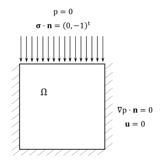
Figure 1: Computational domain and boundary conditions corresponding to the second test problem.

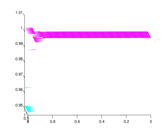
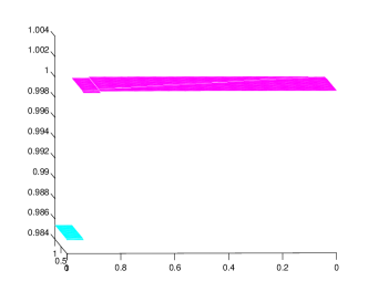
(a)	(b)

Figure 2: Numerical solution for the pressure to the second numerical experiment (a) without mass lumping and (b) with mass lumping.

Here we aim to illustrate the stabilization effect of the mass-lumping performed in the Raviart-Thomas-Nédélec space (see (2.7)). As oscillations of the pressure usually occur when the material has low permeability and for a short time interval, we set the final time as $T=10^{-3}$ and perform only one time step. The value of the permeability is $\kappa=10^{-6}$ and the rest of the material parameters (Lamé coefficients) are $\lambda=12500$ and $\mu=8333$.

In Figure 2(a), we show the approximation for the pressure field obtained without mass lumping. We clearly observe small oscillations close to the boundary where the load is applied. Introducing mass lumping in computing the fluid flux completely removes these oscillations. This is also clearly seen in Figure 2(b).

Another test is illustrated in Figure 3(a)-(b). We show the numerical solutions for the same problem but with variable permeability, i.e. $\kappa(x)=10^{-3}$, $x\in((0,0.5]\times(0,0.5])\cup([0.5,1)\times[0.5,1))$ and $\kappa=1$ in the rest of the domain. While the small oscillations in the solution shown in Figure 3(a) are difficult to see, the lumped mass solution shown in Figure 3(b) is clearly oscillation free.

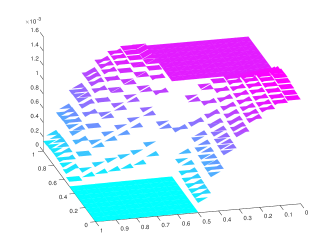
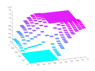
(a)	(b)

Figure 3: Numerical solution for the pressure for the example with variable permeability: (a) without mass lumping and (b) with mass lumping.

Finally, let us remark that, while illustrating that the mass-lumping techniques remove the oscillations in the numerical solution, even in this simple case there is no supporting theory showing that the discretization we have analyzed is in fact monotone and will provide oscillation free approximation to the pressure. This is a difficult and interesting mathematical question which is still open.

5 Conclusions

In this paper, we have proposed a nonconforming finite element method for the three-field formulation for the Biot’s model. We use the lowest order finite elements: piecewise constant for the pore pressure paired with the lowest order Raviart-Thomas-Nédélec elements for the Darcy’s velocity and the nonconforming Crouzeix-Raviart elements for the displacements. The time discretization is an implicit (backward) Euler method. The results on stability and error estimates, however, hold for other implicit time stepping methods as well. For the resulting fully discrete scheme, we have shown uniform inf-sup condition for the discrete problem. Further, based on standard decomposition of the error for the time-dependent problem, we derived optimal order error estimates in both space and time. Finally, we presented numerical tests confirming the theoretical estimates, and, in addition showing that the mass lumping technique to eliminate the Darcy velocity leads to an oscillation-free approximation of the pressure.

6 Acknowledgements

Ludmil Zikatanov gratefully acknowledges the support for this work from the Department of Mathematics at Tufts University and the Applied Mathematics Department at University of Zaragoza.

References

References

- [1] K. Terzaghi, Theoretical Soil Mechanics, Wiley: New York, 1943.
- [2] M. A. Biot, General theory of three‐dimensional consolidation, Journal of Applied Physics 12 (2) (1941) 155–164.
- [3] M. A. Biot, Theory of elasticity and consolidation for a porous anisotropic solid, Journal of Applied Physics 26 (2) (1955) 182–185.
-
[4]
F. J. Gaspar, F. J. Lisbona, P. N. Vabishchevich,
A finite difference
analysis of Biot’s consolidation model, Appl. Numer. Math. 44 (4) (2003)
487–506.
doi:10.1016/S0168-9274(02)00190-3.
URL http://dx.doi.org/10.1016/S0168-9274(02)00190-3 - [5] M. Ferronato, N. Castelletto, G. Gambolati, A fully coupled 3-d mixed finite element model of Biot consolidation, J. Comput. Phys. 229 (12) (2010) 4813–4830.
- [6] J. B. Haga, H. Osnes, H. P. Langtangen, On the causes of pressure oscillations in low-permeable and low-compressible porous media, International Journal for Numerical and Analytical Methods in Geomechanics 36 (12) (2012) 1507–1522.
-
[7]
M. Favino, A. Grillo, R. Krause,
A stability
condition for the numerical simulation of poroelastic systems, in:
C. Hellmich, B. Pichler, D. Adam (Eds.), Poromechanics V: Proceedings of the
Fifth Biot Conference on Poromechanics, 2013, pp. 919–928.
URL http://ascelibrary.org/doi/abs/10.1061/9780784412992.110 - [8] P. Phillips, M. Wheeler, Overcoming the problem of locking in linear elasticity and poroelasticity: an heuristic approach, Computational Geosciences 13 (1) (2009) 5–12.
-
[9]
M. A. Murad, A. F. D. Loula,
Improved accuracy in
finite element analysis of Biot’s consolidation problem, Comput. Methods
Appl. Mech. Engrg. 95 (3) (1992) 359–382.
doi:10.1016/0045-7825(92)90193-N.
URL http://dx.doi.org/10.1016/0045-7825(92)90193-N -
[10]
M. A. Murad, A. F. D. Loula, On
stability and convergence of finite element approximations of Biot’s
consolidation problem, Internat. J. Numer. Methods Engrg. 37 (4) (1994)
645–667.
doi:10.1002/nme.1620370407.
URL http://dx.doi.org/10.1002/nme.1620370407 -
[11]
M. A. Murad, V. Thomée, A. F. D. Loula,
Asymptotic behavior of semidiscrete
finite-element approximations of Biot’s consolidation problem, SIAM J.
Numer. Anal. 33 (3) (1996) 1065–1083.
doi:10.1137/0733052.
URL http://dx.doi.org/10.1137/0733052 -
[12]
G. Aguilar, F. Gaspar, F. Lisbona, C. Rodrigo,
Numerical stabilization of Biot’s
consolidation model by a perturbation on the flow equation, Internat. J.
Numer. Methods Engrg. 75 (11) (2008) 1282–1300.
doi:10.1002/nme.2295.
URL http://dx.doi.org/10.1002/nme.2295 - [13] C. Rodrigo, F. Gaspar, X. Hu, L. Zikatanov, Stability and monotonicity for some discretizations of the biot’s consolidation model, Computer Methods in Applied Mechanics and Engineering 298 (2016) 183–204.
-
[14]
D. N. Arnold, F. Brezzi, M. Fortin,