A Kernelized Stein Discrepancy for Goodness-of-fit Tests

Appendix for “A Kernelized Stein Discrepancy for Goodness-of-fit Tests”

Abstract

We derive a new discrepancy statistic for measuring differences between two probability distributions based on combining Stein’s identity with the reproducing kernel Hilbert space theory. We apply our result to test how well a probabilistic model fits a set of observations, and derive a new class of powerful goodness-of-fit tests that are widely applicable for complex and high dimensional distributions, even for those with computationally intractable normalization constants. Both theoretical and empirical properties of our methods are studied thoroughly.

1 Introduction

Evaluating the goodness-of-fit of models over observed data is a fundamental task in machine learning and statistics. Traditional approaches often involve calculating or comparing the likelihoods or cumulative distribution functions (CDF) of the models. Unfortunately, modern learning techniques increasingly involve complex probabilistic models with computationally intractable likelihoods or CDFs, such as large graphical models, hidden variables models and deep generative models (Koller & Friedman, 2009; Salakhutdinov, 2015). Although Markov chain Monte Carlo (MCMC) or variational methods can be used to approximate the likelihood, their approximation errors are often large and hard to estimate, making it difficult to give results with calibrated statistical significance. In fact, it is often a #P-complete problem to calculate or even approximate likelihoods for graphical models (e.g, Chandrasekaran et al., 2008), making likelihood-based approaches fundamentally infeasible.

We propose a likelihood-free approach for model evaluation with guaranteed statistical significance. In particular, we consider the setting of goodness-of-fit testing, where we test whether a given sample $\{x_{i}\}\sim p(x)$ is drawn from a given distribution $q(x)$, meaning $H_{0}:p=q$. Our method is based on a new discrepancy measure between distributions that can be empirically estimated using $U$-statistics, and depends on $q$ only through its score function ${\boldsymbol{s}}_{q}=\nabla_{x}\log q(x)$; this score function does not depend on the normalization constant in $q(x)$, and can often be calculated efficiently even when the likelihood is intractable. This allows us to apply our methods to complex and high dimensional models on which the likelihood-based methods, or other traditional goodness-of-fit tests, such as $\chi^{2}$-test and Kolmogorov-Smirnov test, can not be applied.

Main Idea

Our method is motivated by Stein’s method and the reproducing kernel Hilbert space (RKHS) theory. Stein’s method (Stein, 1972) is a general theoretical tool for obtaining bounds on distances between distributions. Roughly speaking, it relies on the basic fact that two smooth densities $p(x)$ and $q(x)$ supported on $\mathbb{R}$ are identical if and only if

$$\mathbb{E}_{p}[{\boldsymbol{s}}_{q}(x)f(x)+\nabla_{x}f(x)]=0$$ (1)

for smooth functions $f(x)$ with proper zero-boundary conditions, where ${\boldsymbol{s}}_{q}(x)=\nabla_{x}\log q(x)={\nabla_{x}q(x)}/{q(x)}$ is called the (Stein) score function of $q(x)$; when $p=q$, (1) is known as Stein’s identity (e.g., Stein et al., 2004), and can be proved using integration by parts. As a result, one can define a Stein discrepancy measure between $p$ and $q$ via

$$\mathbb{S}(p,q)=\max_{f\in\mathcal{F}}\big{(}\mathbb{E}_{p}[{\boldsymbol{s}}_{q}(x)f(x)+\nabla_{x}f(x)]\big{)}^{2},$$ (2)

where $\mathcal{F}$ is a set of smooth functions that satisfies (1) and is also rich enough to ensure $\mathbb{S}(p,q)>0$ whenever $p\neq q$. The problem, however, is that $\mathbb{S}(p,q)$ is often computationally intractable because it requires a difficult variational optimization. As a result, $\mathbb{S}(p,q)$ is rarely used in practical machine learning; perhaps the only exception is the recent work of Gorham & Mackey (2015) who obtained a computationally tractable form by enforcing smoothness constraints only on a finite number of points, turning the optimization into a linear programming.

We propose a simpler method for obtaining computational tractable Stein discrepancy $\mathbb{S}(p,q)$ by taking $\mathcal{F}$ to be a ball in a reproducing kernel Hilbert space (RKHS) associated with a smooth positive definite kernel $k(x,x^{\prime})$. In particular, we show that in this case

$$\mathbb{S}(p,q)=\mathbb{E}_{x,x^{\prime}\sim p}\big{[}u_{q}(x,x^{\prime})\big{]},$$ (3)

where $x,x^{\prime}$ are i.i.d. random variables drawn from $p$ and $u_{q}(x,x^{\prime})$ is a function (defined in Theorem 3.6) that depends on $q$ only through the score function $\nabla_{x}\log q(x)$ which can be calculated efficiently even when $q$ has an intractable normalization constant. Specifically, assuming $q(x)=f(x)/Z$ with $Z=\int f(x)dx$ being the normalization constant, we have ${\boldsymbol{s}}_{q}=\nabla_{x}\log f(x)$, independent of $Z$; calculating $Z$ involves a high dimension integration, and has been the major challenge for likelihood-based and Bayesian methods for model evaluation.

With an i.i.d. sample $\{x_{i}\}$ drawn from the (unknown) $p(x)$, the form (3) also enables efficient empirical estimation of $\mathbb{S}(p,q)$ via a $U$-statistic,

$$\hat{\mathbb{S}}(p,q)=\frac{1}{n(n-1)}\sum_{i\neq j}u_{q}(x_{i},x_{j}).$$ (4)

The distribution of $\hat{\mathbb{S}}(p,q)$ can be well characterized using the theory of $U$-statistics (Hoeffding, 1948; Serfling, 2009), allowing us to reduce the testing of $p=q$ to

$$H_{0}:\mathbb{E}_{p}[u_{q}(x,x^{\prime})]=0 vs. H_{1}:\mathbb{E}_{p}[u_{q}(x,x^{\prime})]>0.$$

Related Work

The same idea was independently proposed by Chwialkowski et al. (2016) that appears simultaneously in this proceeding. The technique of combining Stein’s identity with RKHS was first developed by Oates et al. (2014, 2017, 2016) for variance reduction. Reviews of classical goodness-of-fit tests can be found in e.g., Lehmann & Romano (2006), where most methods have computational difficulty for unnormalized distributions. One exception is Fan et al. (2012), which uses the identity $\mathbb{E}_{q}[\boldsymbol{{\boldsymbol{s}}}_{q}]=0$ without using RKHS, but can be inconsistent in power since there exists $q\neq p$ with $\mathbb{E}_{p}[\boldsymbol{{\boldsymbol{s}}}_{q}]=0$.

Outline

Section 2 introduces RKHS and Stein’s identity. Section 3 defines our KSD and studies its main properties, and Section 4 discusses the empirical estimation of KSD and its application in goodness-of-fit tests. We discuss related methods in Section 5, present experiments in Section 6 and conclude the paper in Section 7.

Notations

We denote by $\mathcal{X}$ a subset of $d$-dimensional real space $\mathbb{R}^{d}$. For a vector-valued function $\boldsymbol{f}(x)=[f_{1}(x),\ldots,f_{d^{\prime}}(x)]$, its derivative $\nabla_{x}\boldsymbol{f}(x)=[\frac{\partial f_{j}(x)}{\partial x_{i}}]_{ij}$ is a $d\times d^{\prime}$ matrix-valued function. For a two-variable function (kernel) $k(x,x^{\prime})$, we use $k(\cdot,x^{\prime})=k_{x^{\prime}}(\cdot)$ to refer to a function of $x$ indexed by fixed $x^{\prime}$. For technical simplicity, we will assume all the functions we encounter are absolutely integrable, so that the Fubini-Tonelli theorem can be used to exchange the orders of integrals and infinite sums.

2 Backgrounds

We first introduce positive definite kernels and reproducing kernel Hilbert spaces (RKHS) in Section 2.1, and then Stein’s identity and operator in Section 2.2.

2.1 Kernels and Reproducing Kernel Hilbert Spaces

Let $k(x,x^{\prime})$ be a positive definite kernel. The spectral decomposition of $k(x,x^{\prime})$, as implied by Mercer’s theorem, is defined as

$$k(x,x^{\prime})=\sum_{j}\lambda_{j}e_{j}(x)e_{j}(x^{\prime}),$$ (5)

where $\{e_{j}\}$, $\{\lambda_{j}\}$ are the orthonormal eigenfunctions and positive eigenvalues of $k(x,x^{\prime})$, respectively, satisfying $\int e_{i}(x)e_{j}(x)dx=\mathbb{I}[i=j]$, for $\forall i,j$.

For a positive definite kernel $k(x,x^{\prime})$, its related RKHS $\mathcal{H}$ comprises of linear combinations of its eigenfunctions, i.e., $f(x)=\sum_{j}f_{j}e_{j}(x)$ with $\sum_{j}f_{j}^{2}/\lambda_{j}<\infty$, endowed with an inner product $\langle f,g\rangle_{\mathcal{H}}=\sum_{j}f_{j}g_{j}/\lambda_{j}$ between $f(x)$ and $g(x)=\sum_{j}g_{j}e_{j}(x)$. Thus this Hilbert space is equipped with a norm $||f||_{\mathcal{H}}$ where $||f||_{\mathcal{H}}^{2}=\langle f,f\rangle_{\mathcal{H}}=\sum_{j}f_{j}^{2}/\lambda_{j}$. One can verify that $k(x,\cdot)$ is in $\mathcal{H}$ and satisfies the important “reproducing” property,

$$f(x)=\langle f,k(\cdot,x)\rangle_{\mathcal{H}}, k(x,x^{\prime})=\langle k(\cdot,x),k(\cdot,x^{\prime})\rangle_{\mathcal{H}}.$$

Every positive definite kernel $k$ defines a unique RKHS for which $k$ is a reproducing kernel.

We denote by $\mathcal{H}^{d}=\mathcal{H}\times\cdots\mathcal{H}$ the Hilbert space of $d\times 1$ vector-valued functions $\boldsymbol{f}=\{f_{\ell}\colon f_{\ell}\in\mathcal{H}\}_{\ell\in[d]}$, equipped with an inner product $\langle\boldsymbol{f},\boldsymbol{g}\rangle_{\mathcal{H}^{d}}=\sum_{\ell\in[d]}\langle f_{\ell},g_{\ell}\rangle_{\mathcal{H}}$ for $\boldsymbol{f}$ and $\boldsymbol{g}=\{g_{\ell}\}_{\ell\in[d]}$, and norm $||\boldsymbol{f}||_{\mathcal{H}}=\sqrt{\sum_{\ell}||f_{\ell}||_{\mathcal{H}}^{2}}$.

2.2 Stein’s Identity and Operator

Definition 2.1.

Assume that $\mathcal{X}$ is a subset of $\mathbb{R}^{d}$ and $p(x)$ a continuous differentiable (also called smooth) density whose support is $\mathcal{X}$. The (Stein) score function of $p$ is defined as

$${\boldsymbol{s}}_{p}=\nabla_{x}\log p(x)=\frac{\nabla_{x}p(x)}{p(x)}.$$

We say that a function $f\colon\mathcal{X}\to\mathbb{R}$ is in the Stein class of $p$ if $f$ is smooth and satisfies

$$\int_{x\in\mathcal{X}}\nabla_{x}(f(x)p(x))dx=0.$$ (6)

The Stein’s operator of $p$ is a linear operator acting on the Stein class of $p$, defined as

$${\mathcal{A}}_{p}f(x)={\boldsymbol{s}}_{p}(x)f(x)+\nabla_{x}f(x).$$

Note that both ${\boldsymbol{s}}_{p}$ and ${\mathcal{A}}_{p}f$ are $d\times 1$ vector-valued functions mapping from $\mathcal{X}$ to $\mathbb{R}^{d}$. A vector-valued function $\boldsymbol{f}(x)=[f_{1}(x),\ldots,f_{d^{\prime}}(x)]$ is said to be in the Stein class of $p$ if all $f_{i}$, $\forall i\in[d^{\prime}]$ is in the Stein class of $p$. Applying ${\mathcal{A}}_{p}$ on a vector-valued $\boldsymbol{f}(x)$ results a $d\times d^{\prime}$ matrix-valued function, ${\mathcal{A}}_{p}\boldsymbol{f}(x)={\boldsymbol{s}}_{p}(x)\boldsymbol{f}(x)^{\top}+\nabla_{x}\boldsymbol{f}(x).$

Remark

The condition (6) can be easily checked using integration by parts or divergence theorem; in particular, when $\mathcal{X}=\mathbb{R}^{d}$, (6) holds if

$$\lim_{||x||\to\infty}f(x)p(x)=0,$$

which holds, for example, if $p(x)$ is bounded and $\lim_{||x||\to\infty}f(x)=0$. When $\mathcal{X}$ is a compact subset of $\mathbb{R}^{d}$ with piecewise smooth boundary $\partial\mathcal{X}$, then by divergence theorem (Marsden & Tromba, 2003), (6) holds if $f(x)p(x)=0$ for $\forall x\in\partial\mathcal{X}$, or more generally if $\oint_{\partial\mathcal{X}}p(x)f(x)\cdot\vec{n}(x)dS(x)=0,$ where $\vec{n}(x)$ is the unit normal to the boundary $\partial\mathcal{X}$; $\oint_{\partial}dS(x)$ denotes the surface integral over $\partial\mathcal{X}$.

Lemma 2.2 (Stein’s Identity).

Assume $p(x)$ is a smooth density supported on $\mathcal{X}$, then

$$\mathbb{E}_{p}[{\mathcal{A}}_{p}\boldsymbol{f}(x)]=\mathbb{E}_{p}[{\boldsymbol{s}}_{p}(x)\boldsymbol{f}(x)^{\top}+\nabla\boldsymbol{f}(x)]=0,$$

for any $\boldsymbol{f}$ that is in the Stein class of $p$.

Proof.

By the definition of the Stein class, simply note that ${\boldsymbol{s}}_{p}(x)\boldsymbol{f}(x)^{\top}+\nabla\boldsymbol{f}(x)=\nabla_{x}(\boldsymbol{f}(x)p(x))/p(x).$ ∎

The following result gives a convenient tool for our derivation; it relates the expectation under $p$ of Stein’s operator ${\mathcal{A}}_{q}f$ with the difference of the score functions of $p$ and $q$.

Lemma 2.3 (Ley & Swan (2013)).

Assume $p(x)$ and $q(x)$ are smooth densities supported on $\mathcal{X}$ and $\boldsymbol{f}(x)$ is in the Stein class of $p$, we have

$$\mathbb{E}_{p}[{\mathcal{A}}_{q}\boldsymbol{f}(x)]=\mathbb{E}_{p}[({\boldsymbol{s}}_{q}(x)-{\boldsymbol{s}}_{p}(x))\boldsymbol{f}(x)^{\top}].$$

Proof.

Since $\mathbb{E}_{p}[{\mathcal{A}}_{p}\boldsymbol{f}(x)]=0$, we have $\mathbb{E}_{p}[{\mathcal{A}}_{q}\boldsymbol{f}(x)]=\mathbb{E}_{p}[{\mathcal{A}}_{q}\boldsymbol{f}(x)-{\mathcal{A}}_{p}\boldsymbol{f}(x)]=\mathbb{E}_{p}[({\boldsymbol{s}}_{q}(x)-{\boldsymbol{s}}_{p}(x))\boldsymbol{f}(x)^{\top}].$ ∎

Therefore, $\mathbb{E}_{p}[{\mathcal{A}}_{q}\boldsymbol{f}(x)]$ is the $\boldsymbol{f}(x)$-weighted expectation of the score function difference $({\boldsymbol{s}}_{q}(x)-{\boldsymbol{s}}_{p}(x))$ under $p$. When $\boldsymbol{f}(x)$ is a $d\times 1$ vector-valued function, $\mathbb{E}_{p}[{\mathcal{A}}_{q}\boldsymbol{f}(x)]$ is a $d\times d$ matrix; taking its trace gives a scalar

$$\mathbb{E}_{p}[\mathrm{trace}({\mathcal{A}}_{q}\boldsymbol{f}(x))]=\mathbb{E}_{p}[({\boldsymbol{s}}_{q}(x)-{\boldsymbol{s}}_{p}(x))^{\top}\boldsymbol{f}(x)],$$

which was first derived in Gorham & Mackey (2015) using Langevin diffusion. It is an interesting direction to consider the possibility of using determinant or other matrix norms instead of the trace.

3 Kernelized Stein Discrepancy

We introduce our kernelized Stein discrepancy (KSD) with an elementary definition motivated by Lemma 2.3, and then establish its connection with Stein’s method and RKHS.

Definition 3.1.

A kernel $k(x,x^{\prime})$ is said to be integrally strictly positive definition, if for any function $g$ that satisfies $0<||g||_{2}^{2}<\infty$,

$$\int_{\mathcal{X}}g(x)k(x,x^{\prime})g(x^{\prime})dxdx^{\prime}>0.$$ (7)

Definition 3.2.

The kernelized Stein discrepancy (KSD) $\mathbb{S}(p,q)$ between distribution $p$ and $q$ is defined as

$$\mathbb{S}(p,q)=\mathbb{E}_{x,x^{\prime}\sim p}[\boldsymbol{\delta}_{q,p}(x)^{\top}k(x,x^{\prime})\boldsymbol{\delta}_{q,p}(x^{\prime})],$$ (8)

where $\boldsymbol{\delta}_{q,p}(x)={\boldsymbol{s}}_{q}(x)-{\boldsymbol{s}}_{p}(x)$ is the score difference between $p$ and $q$, and $x$, $x^{\prime}$ are i.i.d. draws from $p(x)$.

Proposition 3.3.

Define $\boldsymbol{g}_{p,q}(x)=p(x)({\boldsymbol{s}}_{q}(x)-{\boldsymbol{s}}_{p}(x))$. Assume $k(x,x^{\prime})$ is integrally strictly positive definite, and $p$, $q$ are continuous densities with $||\boldsymbol{g}_{p,q}||_{2}^{2}<\infty$, we have $\mathbb{S}(p,q)\geq 0$ and $\mathbb{S}(p,q)=0$ if and only if $p=q$.

Proof.

Result directly follows the definition in (7). ∎

This establishes $\mathbb{S}(p,q)$ as a valid discrepancy measure. The requirement that $||\boldsymbol{g}_{p,q}||_{2}^{2}<\infty$ is a mild condition and can easily hold, e.g., when the tail of $p(x)$ decays exponentially, but it may not hold when $p(x)$ has a heavy tail.

The $\mathbb{S}(p,q)$ as defined in (8) requires to know both ${\boldsymbol{s}}_{p}$ and ${\boldsymbol{s}}_{q}$; we now apply Stein’s identity to derive the more convenient form (3) that only requires ${\boldsymbol{s}}_{q}$.

Definition 3.4.

A kernel $k(x,x^{\prime})$ is said to be in the Stein class of $p$ if $k(x,x^{\prime})$ has continuous second order partial derivatives, and both $k(x,\cdot)$ and $k(\cdot,x)$ are in the Stein class of $p$ for any fixed $x$.

It is easy to check that the RBF kernel $k(x,x^{\prime})=\exp(-\frac{1}{2h^{2}}{||x-x^{\prime}||^{2}_{2}})$ is in the Stein class for smooth densities supported on $\mathcal{X}=\mathbb{R}^{d}$.

Proposition 3.5.

If $k(x,x^{\prime})$ is in the Stein class of $p$, so is any $f\in\mathcal{H}$.

Theorem 3.6.

Assume $p$ and $q$ are smooth densities and $k(x,x^{\prime})$ is in the Stein class of $p$. Define

$$u_{q}(x,x^{\prime})={\boldsymbol{s}}_{q}(x)^{\top}k(x,x^{\prime}){\boldsymbol{s}}_{q}(x^{\prime})+{\boldsymbol{s}}_{q}(x)^{\top}\nabla_{x^{\prime}}k(x,x^{\prime})+$$

$$~{}~{}~{}~{}~{}~{}~{}~{}~{}~{}~{}~{}~{}~{}~{}~{}~{}~{}~{}+\nabla_{x}k(x,x^{\prime})^{\top}{\boldsymbol{s}}_{q}(x^{\prime})+\mathrm{trace}(\nabla_{x,x^{\prime}}k(x,x^{\prime})).$$

then $$\mathbb{S}(p,q)=\mathbb{E}_{x,x^{\prime}\sim p}[u_{q}(x,x^{\prime})].$$ (9)

Proof.

Apply Lemma 2.3 twice, first on $k(\cdot,x^{\prime})$ for fixed $x^{\prime}$, and then with fixed $x$. See the Appendix. ∎

The representation in (9) is of central importance for our framework, since it provides a tractable formula for empirical evaluation of $\mathbb{S}(p,q)$ and its confidence interval based on the sample $\{x_{i}\}\sim p$ and score function ${\boldsymbol{s}}_{q}$; see Section 4 for further discussion. An equivalent result of Theorem 3.6 was first presented in Theorem 1 of Oates et al. (2014).

Using the spectral decomposition of $k(x,x^{\prime})$, we can show that $\mathbb{S}(p,q)$ is effectively applying Stein’s operator simultaneously on all the eigenfunctions $e_{j}(x)$ of $k(x,x^{\prime})$.

Theorem 3.7.

Assume $k(x,x^{\prime})$ is a positive definite kernel in the Stein class of $p$, with positive eigenvalues $\{\lambda_{j}\}$ and eigenfunctions $\{e_{j}(x)\}$, then $u_{q}(x,x^{\prime})$ is also a positive definite kernel, and can be rewritten into

$$u_{q}(x,x^{\prime})=\sum_{j}\lambda_{j}~{}[{\mathcal{A}}_{q}e_{j}(x)]^{\top}~{}[{\mathcal{A}}_{q}{e_{j}(x^{\prime})}],$$ (10)

where ${\mathcal{A}}_{q}e_{j}(x)={\boldsymbol{s}}_{q}(x)e_{j}(x)+\nabla_{x}e_{j}(x)$ is the Stein’s operator acted on $e_{j}$. In addition,

$$\mathbb{S}(p,q) =\sum_{j}\lambda_{j}||\mathbb{E}_{x\sim p}[{\mathcal{A}}_{q}e_{j}(x)]||^{2}_{2}.$$ (11)

Note that although $\{e_{j}\}$ are orthonormal, the $\{{\mathcal{A}}_{q}e_{j}(x)\}$ are no longer orthonormal in general.

Finally, we are ready to establish the variational interpretation of $\mathbb{S}(p,q)$ that motivated this work, that is, it can be treated as the maximum of $\mathbb{E}_{x\sim p}[{\mathcal{A}}_{q}f(x)]$ when optimizing $f$ in the unit ball of RKHS $\mathcal{H}$ related to kernel $k(x,x^{\prime})$.

Theorem 3.8.

Let $\mathcal{H}$ be the RKHS related to a positive definite kernel $k(x,x^{\prime})$ in the Stein class of $p$. Denote by $\boldsymbol{\beta}(x^{\prime})=\mathbb{E}_{x\sim p}[{\mathcal{A}}_{q}k_{x^{\prime}}(x)]$, then

$$\mathbb{S}(p,q)=||\boldsymbol{\beta}||_{\mathcal{H}^{d}}^{2}.$$ (12)

Further, we have $\langle\boldsymbol{f},\boldsymbol{\beta}\rangle_{\mathcal{H}^{d}}=\mathbb{E}_{x}[\mathrm{trace}({\mathcal{A}}_{q}\boldsymbol{f})]$ for $\boldsymbol{f}\in\mathcal{H}^{d}$, and hence

$$\sqrt{\mathbb{S}(p,q)} =\max_{\boldsymbol{f}\in\mathcal{H}^{d}}\bigg{\{}\mathbb{E}_{x}[\mathrm{trace}({\mathcal{A}}_{q}\boldsymbol{f})]~{}~{}~{}~{}s.t.~{}~{}~{}~{}||\boldsymbol{f}||_{\mathcal{H}^{d}}\leq 1\bigg{\}}$$ (13)

where the maximum is achieved when $\boldsymbol{f}=\boldsymbol{\beta}/||\boldsymbol{\beta}||_{\mathcal{H}^{d}}$.

Note that (13) is slightly different from the definition in Gorham & Mackey (2015) which do not use the square root; we can take the square root off by optimizing within the ball of $||\boldsymbol{f}||_{\mathcal{H}^{d}}^{2}\leq\mathbb{S}(p,q)$ instead.

4 Goodness-of-fit Testing Based on KSD

The form in (9) allows efficient estimation of $\mathbb{S}(p,q)$ in practice. Given i.i.d. sample $\{x_{i}\}$ drawn from an unknown $p$ and the score function ${\boldsymbol{s}}_{q}(x)$, we can estimate $\mathbb{S}(p,q)$ by

$$\hat{\mathbb{S}}_{u}(p,q)=\frac{1}{n(n-1)}\sum_{1\leq i\neq j\leq n}u_{q}(x_{i},x_{j}),$$ (14)

where $\hat{\mathbb{S}}_{u}(p,q)$ is a form of $U$-statistics (“$U$” stands for unbiasedness), which provides a minimum-variance unbiased estimator for $\mathbb{S}(p,q)$ (Hoeffding, 1948; Serfling, 2009). We can also estimate $\mathbb{S}(p,q)$ using a $V$-statistic of form $\frac{1}{n^{2}}\sum_{i,j=1}^{n}u_{q}(x_{i},x_{j})$, which provides a biased estimator, but has the advantage of always being nonnegative since $u_{q}(x,x^{\prime})$ is positive definite. We will focus on the $U$-statistic in this work because of its unbiasedness.

Theorem 4.1.

Let $k(x,x^{\prime})$ be a positive definite kernel in the Stein class of $p$ and $q$. Assume the conditions in Proposition 3.3 holds, and $\mathbb{E}_{x,x^{\prime}\sim p}[u_{q}(x,x^{\prime})^{2}]<\infty$, we have

1) If $p\neq q$, then $\hat{\mathbb{S}}_{u}(p,q)$ is asymptotically normal with

$$\sqrt{n}(\hat{\mathbb{S}}_{u}(p,q)-\mathbb{S}(p,q))\overset{d}{\to}\mathcal{N}(0,\sigma_{u}^{2}),$$

where $\sigma_{u}^{2}=\mathrm{var}_{x\sim p}(\mathbb{E}_{x^{\prime}\sim p}[u_{q}(x,x^{\prime})])$ and $\sigma_{u}^{2}\neq 0$.

2) If $p=q$, then we have $\sigma_{u}^{2}=0$ (the $U$-statistics is degenerate) and

$$n\hat{\mathbb{S}}_{u}(p,q)\overset{d}{\to}\sum_{j=1}^{\infty}c_{j}(Z_{j}^{2}-1),$$ (15)

where $\{Z_{j}\}$ are i.i.d. standard Gaussian random variables, and $\{c_{j}\}$ are the eigenvalues of kernel $u_{q}(x,x^{\prime})$ under $p(x)$, that is, they are the solutions of $c_{j}\phi_{j}(x)=\int_{x^{\prime}}u_{q}(x,x^{\prime})\phi_{j}(x^{\prime})p(x^{\prime})dx^{\prime}$ for non-zero $\phi_{j}$.

Proof.

Using the standard asymptotic results of $U$-statistics in Serfling (2009, Section 5.5), we just need to check that $\sigma_{u}^{2}\neq 0$ when $p\neq q$ and $\sigma_{u}^{2}=0$ when $p=q$. See Appendix for details. ∎

Theorem 4.1 suggests that $n\hat{\mathbb{S}}_{u}(p,q)$ has a well defined limit distribution under the null $p=q$, that is, $n\hat{\mathbb{S}}_{u}(p,q)<\infty$ with probability one, but grows to $\infty$ at a $\sqrt{n}$-rate under any fixed alternative hypothesis $q\neq p$. This suggests a straightforward goodness-of-fit testing procedure: Denote by $F_{n\hat{\mathbb{S}}_{u}}$ the CDF of $n\hat{\mathbb{S}}_{u}$ under the null $p=q$, and set $\gamma_{1-\alpha}$ the $1-\alpha$ quantile of $F_{n\hat{\mathbb{S}}_{u}}$, i.e., $\gamma_{1-\alpha}=\inf\{s\colon F_{n\hat{\mathbb{S}}_{u}}(s)\geq 1-\alpha\}$, then we reject the null with significant level $\alpha$ if $n\hat{\mathbb{S}}_{u}\geq\gamma_{1-\alpha}$.

Proposition 4.2.

Assume the conditions in Theorem 4.1. For any fixed $q\neq p$, the limiting power of the test that rejects the null $p=q$ when $n\hat{\mathbb{S}}_{u}(p,q)>\gamma_{1-\alpha}$ is one, that is, the test is consistent in power against any fixed $q\neq p$.

One difficulty in implementing this test is that the limit distribution in (15) and its $\alpha$-quantile does not have analytic form unless $c_{j}=0,$ or $1$. Fortunately, the same type of asymptotics appears in many other classical goodness-of-fit tests, such as Cramer-von Mises test, Anderson-Darling test, as well as two-sample tests (Gretton et al., 2012). As a consequence, a line of work has been devoted to approximating the critical values of (15), including bootstrap methods (Arcones & Gine, 1992; Huskova & Janssen, 1993; Chwialkowski et al., 2014) and eigenvalue approximation (Gretton et al., 2009).

Algorithm 1 Bootstrap Goodness-of-fit Test based on KSD

  Input: Sample $\{x_{i}\}$ and score function ${\boldsymbol{s}}_{q}(x)=\nabla_{x}\log q(x)$. Bootstrap sample size $m$.

  Test: $H_{0}$: $\{x_{i}\}$ is drawn from $q$    v.s    $H_{1}$: $\{x_{i}\}$ is not drawn from $q$.

  1. Compute $\hat{\mathbb{S}}_{u}$ by (14) and $u_{q}(x,x^{\prime})$ as defined in Theorem 3.6. Generate $m$ bootstrap sample $\hat{\mathbb{S}}^{*}_{u}$ by (16).

  2. Reject $H_{0}$ with significance level $\alpha$ if the percentage of $\hat{\mathbb{S}}^{*}_{u}$ that satisfies $\hat{\mathbb{S}}^{*}_{u}>\hat{\mathbb{S}}_{u}$ is less than $\alpha$.

In this work, we adopt the bootstrap method suggested in Huskova & Janssen (1993); Arcones & Gine (1992): We repeatedly draw multinomial random weights $(w_{1},\ldots w_{n})\sim~{}\mathrm{Mult}(n~{};~{}\frac{1}{n},\ldots,\frac{1}{n})$, and calculate bootstrap sample

$$\hat{\mathbb{S}}^{*}_{u}(p,q)=\sum_{i\neq j}(w_{i}-\frac{1}{n})(w_{j}-\frac{1}{n})u_{q}(x_{i},x_{j}),$$ (16)

and then calculate the empirical quantile $\hat{\gamma}_{1-\alpha}$ of $n\hat{\mathbb{S}}^{*}_{u}(p,q)$. The consistency of $\hat{\gamma}_{1-\alpha}$ for degenerate $U$-statistics has been established in Arcones & Gine (1992); Huskova & Janssen (1993).

Theorem 4.3 (Huskova & Janssen (1993)).

Assume the conditions in Theorem 4.1. If $p=q$, then as the bootstrap sample size $m\to\infty$,

$$\sup_{s\in\mathbb{R}}\big{|}~{}\mathrm{Pr}(n\hat{\mathbb{S}}^{*}_{u}\leq s~{}|~{}\{x_{i}\}_{i=1}^{n})~{}-~{}\mathrm{Pr}(n\hat{\mathbb{S}}_{u}\leq s)~{}\big{|}\to 0,$$

that is, the bootstrap test attains the correct significance level asymptotically (consistent in level).

It is important to note, on the other hand, that the more usual bootstrap, such as $\sum_{i\neq j}w_{i}w_{j}u_{q}(x_{i},x_{j})$, may not work for degenerate $U$-statistics as discussed in Arcones & Gine (1992).

This bootstrap test is summarized in Algorithm 1; its cost is $O(mn^{2})$ where $n$ is the size of the sample $\{x_{i}\}$ and $m$ the bootstrap sample size. A more computationally efficient, but less statistically powerful, method can be constructed based on the following linear estimator:

$$\hat{\mathbb{S}}_{lin}=\frac{1}{\lfloor n/2\rfloor}\sum_{i=1}^{\lfloor n/2\rfloor}u_{q}(x_{2i-1},x_{2i}),$$ (17)

which has a zero-mean Gaussian limit under the null. This gives a test with only $O(n)$ time complexity: reject the null if $\hat{\mathbb{S}}_{lin}>\hat{\sigma}z_{1-\alpha}$, where $z_{1-\alpha}$ is the $1-\alpha$ quantile of the standard Gaussian distribution, and $\hat{\sigma}$ the standard deviation of $\{u_{q}(x_{2i-1},x_{2i})\}$. This test, however, tends to perform much worse than the $U$-statistic based test as we show in our experiments. Further computation-efficiency trade-off between the linear- and $U$-statistic can be obtained by block-wise averaging; see Ho & Shieh (2006); Zaremba et al. (2013) for details.

5 Related Methods

We discuss the connection with Fisher divergence and maximum discrepancy measure (MMD).

5.1 Connection with Fisher Divergence

Fisher divergence, also known as Fisher information distance (Johnson, 2004), is defined as

$$\mathbb{F}(p,q)=\mathbb{E}_{x}\big{[}||\nabla_{x}\log p(x)-\nabla_{x}\log q(x)||^{2}_{2}],$$ (18)

that is, it is the $\mathcal{L}^{2}(p)$ norm of ${\boldsymbol{s}}_{q}(x)-{\boldsymbol{s}}_{p}(x)$. An immediate connection is made by noting that $\mathbb{F}(p,q)$ can be treated as a special case of $\mathbb{S}(p,q)$ defined in (8) with $k(x,x^{\prime})=\mathbb{I}[x=x^{\prime}]$, or a RBF kernel with bandwidth $h\to 0$; in this sense, we can also think KSD as a kernelized version of Fisher divergence. We can establish the follow inequalities between $\mathbb{F}(p,q)$ and $\mathbb{S}(p,q)$:

Theorem 5.1.

1) Following Definition (8) and (18), we have

$$|\mathbb{S}(p,q)|\leq\sqrt{\mathbb{E}_{x,x^{\prime}\sim p}[k(x,x^{\prime})^{2}]}\cdot\mathbb{F}(p,q).$$ (19)

2) In addition, if $k(x,x^{\prime})$ is positive definite and in the Stein class of $p$, and ${\boldsymbol{s}}_{q}-{\boldsymbol{s}}_{p}\in\mathcal{H}^{d}$, we have, for $p\neq q$,

$$\sqrt{\mathbb{S}(p,q)}\geq\mathbb{F}(p,q)~{}/~{}||{\boldsymbol{s}}_{q}-{\boldsymbol{s}}_{p}||_{\mathcal{H}^{d}}.$$ (20)

Proof.

(19) is a simple result of Cauchy-Schwarz inequality, and (20) can be obtained by taking $f=({\boldsymbol{s}}_{q}-{\boldsymbol{s}}_{p})/||{\boldsymbol{s}}_{q}(x)-{\boldsymbol{s}}_{p}(x)||_{\mathcal{H}^{d}}$ in (13). See Appendix. ∎

(19) suggests that the convergence in Fisher divergence is stronger than that in KSD. In fact, using Stein’s method, Ley & Swan (2013) showed that Fisher divergence is stronger than most other divergences, including KL, total variation and Hellinger distances.

In addition, we can also represent $\mathbb{F}(p,q)$ in a variational form similar to (13) but with $\boldsymbol{f}$ optimized over the unit ball of the intersection of the unit ball in $\mathcal{L}^{2}(p)$ space and the Stein class of $p$, which is larger than the ball of $\mathcal{H}^{d}$ and includes discontinuous, non-smooth functions; see Proposition A.1 in Appendix.

Despite the connections, the critical disadvantage of Fisher divergence compared to KSD is that the computationally convenient representation (9) no longer holds for Fisher divergence, because its corresponding kernel $\mathbb{I}[x=x^{\prime}]$ is not differentiable. Therefore, we can not estimate $\mathbb{F}(p,q)$ using the $U$-statistic in (14). Instead, estimating $\mathbb{F}(p,q)$ seems to be substantially more difficult. To see this, note that

$$\mathbb{F}(p,q) =\mathbb{E}_{x\sim p}[||{\boldsymbol{s}}_{q}(x)||^{2}_{2}-2{\boldsymbol{s}}_{p}(x)^{\top}{\boldsymbol{s}}_{q}(x)+||{\boldsymbol{s}}_{p}(x)||_{2}^{2}]$$

$$=\mathbb{E}_{x\sim p}[\phi_{q}(x)]~{}+~{}\mathbb{E}_{x\sim p}||{\boldsymbol{s}}_{p}(x)||_{2}^{2},$$ (21)

where $\phi_{q}(x)=||{\boldsymbol{s}}_{q}(x)||^{2}_{2}+2\mathrm{trace}(\nabla_{x}{\boldsymbol{s}}_{q}(x))$ and is obtained by applying Stein’s identity on the cross term. Note that although the first term $\mathbb{E}_{x\sim p}[\phi_{q}(x)]$ in (21) can be estimated by the empirical mean of $\phi_{q}(x)$ (which only depends on ${\boldsymbol{s}}_{q}$) under sample $\{x_{i}\}\sim p$, the second term $\mathbb{E}_{x\sim p}||{\boldsymbol{s}}_{p}(x)||_{2}^{2}$ is more difficult to estimate, since it depends on the score function ${\boldsymbol{s}}_{p}(x)$ of the unknown $p(x)$, and hence requires a kernel density estimator for $p(x)$; see Hall & Marron (1987); Birge & Massart (1995). We should point out that similar difficult “constant” terms appear in other common discrepancy measures such as KL divergence and $\alpha$-divergence (e.g., Krishnamurthy et al., 2014). For this reason, KSD provides a much more convenient tool for goodness-of-fit tests than the other discrepancies.

Meanwhile, Fisher divergence still has the advantage of being independent of the normalization constants of $p$ and $q$, and provides a useful tool in cases when it does not require evaluating the term ${\boldsymbol{s}}_{p}(x)$. For example, Fisher divergence has been widely used for parameter estimation, finding the optimal $q(x)$ that best fits a sample $\{x_{i}\}$ by minimizing $\mathbb{F}(p,q)$; this yields the score matching methods developed in both parametric (Hyvärinen, 2005; Lyu, 2009) and non-parametric (Sriperumbudur et al., 2013) settings.

5.2 Maximum Mean Discrepancy & Two-sample Tests

Closely related to goodness-of-fit tests are two sample tests, which test whether two i.i.d. samples $\{x_{i}\}$ and $\{y_{i}\}$ are drawn from the same distribution. In principle, one can turn a goodness-of-fit test into a two sample test by drawing $\{y_{i}\}$ from $q(x)$. However, it is often difficult to draw exact i.i.d. samples for practical models, and furthermore MCMC sampling may be computationally expensive, suffer from the convergence problems, and introduce undesired correlations. When the MCMC approximation is poor, the two sample test would reject the null even when $p=q$ (inconsistent in level).

Maximum Mean Discrepancy (Gretton et al., 2012) is a nonparametric distance measure widely used for two sample tests, defined as

$${\mathbb{M}}(p,q)=\max_{h\in\mathcal{H}}\big{\{}\mathbb{E}_{p}[h(x)]-\mathbb{E}_{q}[h(x)]~{}~{}~{}s.t.~{}~{}~{}||h||_{\mathcal{H}}\leq 1\big{\}},$$

where $\mathcal{H}$ is the RKHS of kernel $k(x,x^{\prime})$. Gretton et al. (2012) showed that $\mathbb{M}(p,q)$ can be rewritten into

$$\mathbb{M}(p,q)=\mathbb{E}[k(x,x^{\prime})+k(y,y^{\prime})-2k(x,y^{\prime})],$$ (22)

where $x,x^{\prime}$ and $y,y^{\prime}$ are i.i.d. draws from $p$ and $q$, respectively. Therefore, $\mathbb{M}(p,q)$ can be empirically estimated based on sample $x_{i}\sim p$ and $y_{i}\sim q$ using $U$- or $V$- statistics, making it a useful tool for two sample tests. Our KSD, on the other hand, is better estimated with sample $x_{i}\sim p$ and the score function ${\boldsymbol{s}}_{q}$ and hence suitable for goodness-of-fit tests. Finally, by comparing (22) with (9) and noting that $\mathbb{E}_{x\sim q}[u_{q}(x,x^{\prime})]=0$, we can consider KSD as a special MMD with kernel $u_{q}(x,x^{\prime})$; the key difference is that kernel $u_{q}(x,x^{\prime})$ depends on $q$, making KSD asymmetric.

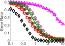
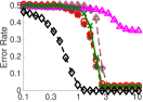
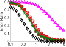
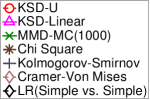
Perturbation Magnitude $\sigma_{per}$	Perturbation Magnitude $\sigma_{per}$	Perturbation Magnitude $\sigma_{per}$
(a) Perturbation on Mean	(b) Perturbation on Variance	(c) Perturbation on Weights
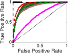
Sample Size $n$	Sample Size $n$	Sample Size $n$	($n=100$, $\sigma_{per}=1$)
(d) Perturbation on Mean	(e) Perturbation on Variance	(f) Perturbation on Weights	(g) Perturbation on Mean

Figure 1: Results on 1D Gaussian mixture. (a)-(c) The error rates of different methods vs. the perturbation magnitude $\sigma_{per}$ when perturbing the mean, variance and mixture weights, respectively; we use a fixed sample size of $n=100$. (d)-(f) the error rates vs. the sample size $n$, with fixed perturbation magnitude $\sigma_{per}=1$. We find that the type I errors of all the methods are well controlled under $0.05$, and hence the reported error rates are essentially type II errors. (g) The ROC curve with mean perturbation, $n=100$, $\sigma_{per}=1$.

6 Experiments

We present empirical results in this section. We start with a toy case of 1D Gaussian mixture on which we can compare with the classical goodness-of-fit tests that only work for univariate distributions, and then proceed to Gaussian-Bernoulli restricted Boltzmann machine (RBM), a graphical model widely used in deep learning (Welling et al., 2004; Hinton & Salakhutdinov, 2006). The following methods are evaluated, all with a significance level of $0.05$:

1) KSD-U. The KSD-based bootstrap test using $U$-statistic in Algorithm 1 (bootstrap size is $1000$), using RBF kernel with bandwidth chosen to be median of the data distances.

2) KSD-Linear. The KSD test based on the linear estimator in (17) with asymptotically normal null distribution.

3) Classical goodness-of-fit tests, including $\chi^{2}$ test, Kolmogorov-Smirnov test and Cramer-von Mises test (Lehmann & Romano, 2006); they are evaluated on only the 1D Gaussian mixture.

4) MMD-MC(${n^{\prime}}$). Draw exact sample $\{y_{i}\}$ of size $n^{\prime}$ from $q(x)$ and perform two sample MMD test of Gretton et al. (2012) over $\{x_{i}\}$ and $\{y_{i}\}$ using bootstrap, with 1000 bootstrap replicates.

5) MMD-MCMC(${n^{\prime}}$). Draw approximate sample $\{y_{i}\}$ of size $n^{\prime}$ from $q(x)$ using Gibbs sampler and perform MMD test on $\{x_{i}\}$ and $\{y_{i}\}$; we use $1000$ burn-in steps.

6) LR (simple vs. simple). We evaluate the exact log-likelihood ratio $2\log(q(x)/p(x))$ and use it to test whether $\{x_{i}\}$ is drawn from $p(x)$ or $q(x)$. This approach is an oracle test in that it knows it exactly calculates the likelihood, and assumes we know $p(x)$ and tests a much easier null hypothesis of simple vs. simple.

7) Likelihood Ratio (AIS). We approximately evaluate the likelihood ratio using annealed importance sampling (AIS), which is one of the most widely used algorithm for approximating likelihood (Neal, 2001; Salakhutdinov & Murray, 2008). Our AIS implementation uses a Gibbs sampler transition with a linear temperature grid of size $1000$. We do not perform a test based on the AIS result because it is hard to know the approximation error.

1D Gaussian Mixture

We draw i.i.d. sample $\{x_{i}\}_{i=1}^{n}$ from $p(x)=\sum_{k=1}^{5}w_{k}\mathcal{N}(x~{};\mu_{k},\sigma^{2})$ with $w_{k}=1/5$, $\sigma=1$ and $\mu_{k}$ randomly drawn from $\mathrm{Uniform}[0,10]$. We then generate $q(x)$ by adding Gaussian noise on $\mu_{k}$, $\log w_{k}$, or $\log\sigma^{2}$, leading to three different ways for perturbation; the perturbation magnitude is controlled by the variance $\sigma_{per}^{2}$ of Gaussian noise. In our experiment, we set $q(x)$ randomly with equal probability to be either the true model $p(x)$ ($H_{0}:p=q$), or the perturbed version ($H_{1}:p\neq q$), and use different methods to test $H_{0}$ vs. $H_{1}$. We repeat $1000$ trials, and report the average error rate in Figure 1.

We find from Figure 1 that the oracle LR (simple vs. simple) performs the best as expected. Otherwise, our KSD-U performs comparably with, or better than, the classical tests ($\chi^{2}$, Kolmogorov-Smirnov and Cramer-Von Mises) as well as MMD-MC(1000). KSD-Linear tends to perform the worst, suggesting it is not useful in this simple setting. However, it can serve as a computationally efficient alternative of KSD-U for more complex models on which the other tests are not practical. Note that because both the cases of $p=q$ and $p\neq q$ happen with $0.5$ probability in our simulation, the error rate in the hardest case when $p$ is close $q$ is $0.5$.

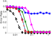
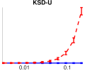
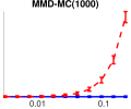
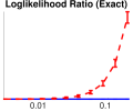
Perturbation Magnitude $\sigma_{per}$	Perturbation Magnitude $\sigma_{per}$	Perturbation Magnitude $\sigma_{per}$	Perturbation Magnitude $\sigma_{per}$
(a)	(c)	(e)	(g)
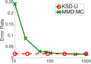
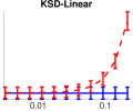
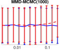
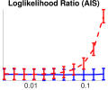
Monte Carlo Sample Size $n^{\prime}$ in MMD	Perturbation Magnitude $\sigma_{per}$	Perturbation Magnitude $\sigma_{per}$	Perturbation Magnitude $\sigma_{per}$
(b)	(d)	(f)	(h)

Figure 2: Results on Gaussian-Bernoulli RBM. (a) The error rate vs. the perturbation magnitude $\sigma_{per}$. (b) The error rate of MMD-MC vs. the size of the exact sample used. (c) Different discrepancy measures between $p$ and $q$ under the null $p=q$ (blue solid lines) and the alternatives $p\neq q$ (dashed red lines); the x-axes are the deviation $\sigma_{per}$ between $p$ and $q$ when $p\neq q$. We set $n=100$ in all the cases.

Gaussian-Bernoulli Restricted Boltzmann Machine (RBM)

Gaussian-Bernoulli RBM is a hidden variable graphical models consist of a continuous observable variable $x\in\mathbb{R}^{d}$ and a binary hidden variable $h\in\{\pm 1\}^{d^{\prime}}$, with joint probability

$$p(x,h)=\frac{1}{Z}\exp(\frac{1}{2}x^{\top}Bh+b^{\top}x+c^{\top}h-\frac{1}{2}||x||^{2}_{2}),$$

where $Z$ is the normalization constant. The probability of the observable variable $x$ is $p(x)=\sum_{h\in\{\pm 1\}^{d^{\prime}}}p(x,h),$ which is intractable to calculate due to the difficult constant term $Z$. Nevertheless, one can show that its score function ${\boldsymbol{s}}_{p}$ can be easily calculated in a closed form,

$${\boldsymbol{s}}_{p}(x)=b-x+B~{}\phi(B^{\top}x+c),~{}~{}~{}~{}~{}~{}~{}\phi(y)=\frac{e^{2y}-1}{e^{2y}+1}.$$

In our experiment, we simulate a true model $p(x)$ by drawing $b$ and $c$ from standard Gaussian and select $B$ uniformly randomly from $\{\pm 1\}$; we use $d=50$ observable variables and $d^{\prime}=10$ hidden variables, so that it remains possible to exactly calculate $p(x)$ and draw exact samples using the brute-force algorithm. Similar to the case of 1D Gaussian mixture, we set $q(x)$ randomly with equal probability to be equal to either $p(x)$ or a perturbed version by adding Gaussian noise to $B$ with variance $\sigma_{per}^{2}$. We report the the error rates of different tests in Figure 2; the results are averaged on $1000$ random trials.

Figure 2(a) shows that the oracle LR (simple vs. simple) performs the best again as expected, followed by our KSD-U method. The MMD-MCMC breaks down because the MCMC sample is not representative of $q$, while the performance of MMD-MC depends on the size of the exact sample: it performs worse than KSD-U with MMD-MC(100), and is almost as good with MMD-MC(1000); see also Figure 2(b). Again, we find that KSD-linear generally performs much worse than KSD-U, but it provides a computationally efficient $O(n)$ alternative to KSD-U which has a $O(mn^{2})$ complexity and MMD which costs $O(mnn^{\prime})$. A trade-off between linear and quadratic complexity can be achieved using block averaging; see Zaremba et al. (2013).

Figure 2(c)-(h) shows the different discrepancy measures under the case $p=q$ and $p\neq q$, respectively. Again, we can find that the exact likelihood ratio provides the best discrimination, while MMD-MCMC fails to distinguish the two cases at all. The AIS approximation performs reasonably well, but is worse than KSD-U and MMD-MC(1000) in this particular case.

7 Conclusion and Future Directions

We propose a new computationally tractable discrepancy measure between complex probability models, and use it to derive a novel class of goodness-of-fit tests. We believe our discrepancy measure provides a new fundamental tool for analyzing and using complex probability models in statistics and machine learning. Future directions include extending our method to composite goodness-of-fit tests, in which we want to test if the observed data follows a given class of distributions, as well as understanding the theoretical discrimination power of KSD compared to the other classical goodness-of-fit tests, two sample tests (e.g., MMD with infinite exact Monte Carlo sample), and the method in Gorham & Mackey (2015).

Acknowledgment

This work is supported in part by NSF CRII 1565796. We thank Arthur Gretton and the anonymous reviewers for their valuable comments.

Appendix A Proofs

Proof of Theorem 3.6.

1) Denote by $\boldsymbol{v}(x,x^{\prime})=k(x,x^{\prime}){\boldsymbol{s}}_{q}(x^{\prime})+\nabla_{x^{\prime}}k(x,x^{\prime})={\mathcal{A}}_{q}k_{x}(x^{\prime})$; applying Lemma 2.3 on $k(x,\cdot)$ with fixed $x$,

$$\mathbb{S}(p,q) =\mathbb{E}_{x,x^{\prime}\sim p}[({\boldsymbol{s}}_{q}(x)-{\boldsymbol{s}}_{p}(x))^{\top}k(x,x^{\prime})({\boldsymbol{s}}_{q}(x^{\prime})-{\boldsymbol{s}}_{p}(x^{\prime}))]$$

$$=\mathbb{E}_{x,x^{\prime}\sim p}[({\boldsymbol{s}}_{q}(x)-{\boldsymbol{s}}_{p}(x))^{\top}\boldsymbol{v}(x,x^{\prime})]$$

Because $k(\cdot,x^{\prime})$ is in the Stein class of $p$ for any $x^{\prime}$, we can show that $\nabla_{x^{\prime}}k(\cdot,x^{\prime})$ is also in the Stein class, since

$$\int_{x}\nabla_{x}(p(x)\nabla_{x^{\prime}}k(x,x^{\prime}))dx=\nabla_{x^{\prime}}\int_{x}\nabla_{x}(p(x)k(x,x^{\prime}))dx=0,$$

and hence $\boldsymbol{v}(\cdot,x^{\prime})$ is also in the Stein class; apply Lemma 2.3 on $\boldsymbol{v}(\cdot,x^{\prime})$ with fixed $x^{\prime}$ gives

$$\mathbb{S}(p,q) =\mathbb{E}_{x,x^{\prime}\sim p}[({\boldsymbol{s}}_{q}(x)-{\boldsymbol{s}}_{p}(x))^{\top}\boldsymbol{v}(x,x^{\prime}))]$$

$$=\mathbb{E}_{x,x^{\prime}\sim p}[{\boldsymbol{s}}_{q}(x)^{\top}\boldsymbol{v}(x,x^{\prime})+\mathrm{trace}(\nabla_{x}\boldsymbol{v}(x,x^{\prime}))]$$

The result then follows by noting that $\nabla_{x}\boldsymbol{v}(x,x^{\prime})=\nabla_{x}k(x,x^{\prime}){\boldsymbol{s}}_{q}(x^{\prime})^{\top}+\nabla_{x^{\prime}x^{\prime}}k(x,x^{\prime}).$ ∎

Proof of Theorem 3.7.

Note that

$$\nabla_{x}k(x,x^{\prime})=\sum_{j}\lambda_{j}\nabla_{x}e_{j}(x)~{}e_{j}(x^{\prime}), \nabla_{x,x^{\prime}}k(x,x^{\prime})=\sum_{j}\lambda_{j}\nabla_{x}e_{j}(x)~{}\nabla_{x^{\prime}}e_{j}(x^{\prime})^{\top},$$

and hence

$$\!\!\!\!\!\!\!\!u_{q}(x,x^{\prime})$$

$$~{}={\boldsymbol{s}}_{q}(x)^{\top}k(x,x^{\prime}){\boldsymbol{s}}_{q}(x^{\prime})+{\boldsymbol{s}}_{q}(x)^{\top}\nabla_{x}^{\prime}k(x,x^{\prime})+{\boldsymbol{s}}_{q}(x^{\prime})^{\top}\nabla_{x}k(x,x^{\prime})+\mathrm{trace}(\nabla_{x,x^{\prime}}k(x,x^{\prime})$$

$$~{}=\sum_{j}\lambda_{j}\big{[}{\boldsymbol{s}}_{q}(x)^{\top}e_{j}(x)e_{j}(x^{\prime}){\boldsymbol{s}}_{q}(x^{\prime})+{\boldsymbol{s}}_{q}(x)^{\top}e_{j}(x)\nabla_{x^{\prime}}e_{j}(x^{\prime})+{\boldsymbol{s}}_{q}(x^{\prime})^{\top}\nabla_{x}e_{j}(x)e_{j}(x^{\prime})+\nabla_{x}e_{j}(x)^{\top}\nabla_{x^{\prime}}e_{j}(x^{\prime})\big{]}$$

$$~{}=\sum_{j}\lambda_{j}\big{[}{\boldsymbol{s}}_{q}(x)e_{j}(x)+\nabla_{x}e_{j}(x)\big{]}^{\top}\big{[}{\boldsymbol{s}}_{q}(x^{\prime})e_{j}(x^{\prime})+\nabla_{x^{\prime}}e_{j}(x^{\prime})\big{]}$$

$$~{}=\sum_{j}\lambda_{j}[{\mathcal{A}}_{q}e_{j}(x)]^{\top}[{\mathcal{A}}_{q}e_{j}(x^{\prime})].$$

Therefore, $u_{q}(x,x^{\prime})$ is positive definite because $\lambda_{j}>0$. In addition,

$$\mathbb{S}(p,q) =\mathbb{E}_{x,x^{\prime}}[u_{q}(x,x^{\prime})]$$

$$=\sum_{j}\lambda_{j}\mathbb{E}_{x}[{\mathcal{A}}_{q}e_{j}(x)]^{\top}~{}\mathbb{E}_{x^{\prime}}[{\mathcal{A}}_{q}e_{j}(x^{\prime})]$$

$$=\sum_{j}\lambda_{j}||\mathbb{E}_{x}[{\mathcal{A}}_{q}e_{j}(x)]||_{2}^{2}.$$

∎

Proof of Theorem 3.8.

We first prove (12) by applying the reproducing property $k(x,x^{\prime})=\langle k(x,\cdot),k(x^{\prime},\cdot)\rangle_{\mathcal{H}}$ on (8):

$$\mathbb{S}(p,q) =\mathbb{E}_{x,x^{\prime}\sim p}[({\boldsymbol{s}}_{q}(x)-{\boldsymbol{s}}_{p}(x))^{\top}~{}k(x,x^{\prime})~{}({\boldsymbol{s}}_{q}(x^{\prime})-{\boldsymbol{s}}_{p}(x^{\prime}))]$$

$$=\mathbb{E}_{x,x^{\prime}\sim p}[({\boldsymbol{s}}_{q}(x)-{\boldsymbol{s}}_{p}(x))^{\top}~{}~{}\big{\langle}k(x,\cdot),~{}k(x,\cdot)\big{\rangle}_{\mathcal{H}}~{}({\boldsymbol{s}}_{q}(x^{\prime})-{\boldsymbol{s}}_{p}(x^{\prime}))]$$

$$=\sum_{\ell=1}^{d}\big{\langle}\mathbb{E}_{x}[({\boldsymbol{s}}_{q}^{\ell}(x)-{\boldsymbol{s}}_{p}^{\ell}(x))k(x,\cdot)],~{}\mathbb{E}_{x^{\prime}}[k(x,\cdot)({\boldsymbol{s}}_{q}^{\ell}(x)-{\boldsymbol{s}}_{p}^{\ell}(x))]\big{\rangle}_{\mathcal{H}}$$

$$=\sum_{\ell=1}^{d}\big{\langle}\boldsymbol{\beta}_{\ell},\boldsymbol{\beta}_{\ell}\big{\rangle}_{\mathcal{H}}$$

$$=||\boldsymbol{\beta}||_{\mathcal{H}^{d}}^{2}$$

where we used the fact that $\boldsymbol{\beta}(x^{\prime})=\mathbb{E}_{x\sim p}[{\mathcal{A}}_{q}k_{x^{\prime}}(x)]=\mathbb{E}_{x\sim p}[({\boldsymbol{s}}_{q}(x)k(x,x^{\prime})+\nabla_{x}k(x,x^{\prime})]=\mathbb{E}_{x}[({\boldsymbol{s}}_{q}(x)-{\boldsymbol{s}}_{p}(x))k(x,x^{\prime})]$. In addition,

$$\langle\boldsymbol{f},\boldsymbol{\beta}\rangle_{\mathcal{H}^{d}} =\sum_{\ell=1}^{d}\langle f_{\ell},~{}\mathbb{E}_{x\sim p}[({\boldsymbol{s}}_{q}^{\ell}(x)k(x,\cdot)+\nabla_{x_{\ell}}k(x,\cdot)]\rangle_{\mathcal{H}}$$

$$=\sum_{\ell=1}^{d}\mathbb{E}_{x\sim p}[({\boldsymbol{s}}_{q}^{\ell}(x)\langle f_{\ell},k(x,\cdot)\rangle_{\mathcal{H}}+\langle f_{\ell},\nabla_{x_{\ell}}k(x,\cdot)\rangle_{\mathcal{H}}]$$

$$=\sum_{\ell=1}^{d}\mathbb{E}_{x\sim p}[({\boldsymbol{s}}_{q}^{\ell}(x)f_{\ell}(x)+\nabla_{x_{\ell}}f_{\ell}(x)]$$

$$=\mathbb{E}_{x\sim p}[\mathrm{trace}({\mathcal{A}}_{q}\boldsymbol{f}(x))],$$

where we used the fact that $\nabla_{x}f(x)=\langle f(\cdot),~{}\nabla_{x}k(x,\cdot)\rangle_{\mathcal{H}}$; see (Zhou, 2008; Steinwart & Christmann, 2008). The variational form (13) then follows the fact that $||\boldsymbol{\beta}||_{\mathcal{H}^{d}}=\max_{\boldsymbol{f}\in\mathcal{H}^{d}}\big{\{}\langle\boldsymbol{f},\boldsymbol{\beta}\rangle_{\mathcal{H}^{d}},~{}~{}~{}.s.t.~{}~{}||\boldsymbol{f}||_{\mathcal{H}^{d}}\leq 1\big{\}}$.

Finally, the $\boldsymbol{\beta}(\cdot)=\mathbb{E}_{x\sim p}[({\boldsymbol{s}}_{q}(x)k(x,\cdot)+\nabla_{x}k(x,\cdot)]$ is in the Stein class of $p$ because $k(x,\cdot)$ and $\nabla_{x}k(x,\cdot)$ are in the Stein class of $p$ for any fixed $x$ (see the proof of Theorem 3.6). ∎

Proof Proposition 3.5.

For any $f\in\mathcal{H}$ with kernel $k(x,x^{\prime})$, we have $f=\langle f,~{}k(\cdot,x)\rangle_{\mathcal{H}}$ and $\nabla_{x}f=\langle f,~{}\nabla_{x}k(x,\cdot)\rangle_{\mathcal{H}}$. Therefore,

$$\mathbb{E}_{x\sim p}[{\boldsymbol{s}}_{p}(x)f(x)+\nabla_{x}f(x)] =\mathbb{E}_{x\sim p}[{\boldsymbol{s}}_{p}(x)\big{\langle}f,~{}k(x,\cdot)\big{\rangle}_{\mathcal{H}}+\big{\langle}f,~{}\nabla_{x}k(x,\cdot)\big{\rangle}_{\mathcal{H}}]$$

$$=\big{\langle}f,~{}~{}\mathbb{E}_{x\sim p}[{\boldsymbol{s}}_{p}(x)k(x,\cdot)+\nabla_{x}k(x,\cdot)]\big{\rangle}_{\mathcal{H}}$$

$$=\big{\langle}f,~{}~{}\mathbb{E}_{x\sim p}[{\mathcal{A}}_{p}k_{x}(\cdot)]\rangle_{\mathcal{H}}$$

$$=0,$$

where the last step used the fact that $\mathbb{E}_{x\sim p}[{\mathcal{A}}_{p}k_{x}(\cdot)]$ because $k_{x}(\cdot)=k(\cdot,x)$ is in the Stein class of $p$ for any fixed $x$. ∎

Proof of Theorem 4.1.

Applying the standard asymptotic results of $U$-statistics in Serfling (2009, Section 5.5), we just need to check that $\sigma_{u}^{2}\neq 0$ when $p\neq q$ and $\sigma_{u}^{2}=0$ when $p=q$.

We first note that we can show that $\mathbb{E}_{x^{\prime}\sim p}[u_{q}(x,x^{\prime})]=\mathrm{trace}({\mathcal{A}}_{q}\boldsymbol{\beta})$, where $\boldsymbol{\beta}(x)=\mathbb{E}_{x^{\prime}\sim p}[{\mathcal{A}}_{q}k_{x}(x^{\prime})]$ and is in the Stein class of $p$ (see the proof of Theorem 3.6). Therefore, when $p=q$, we have $\boldsymbol{\beta}(x)\equiv 0$ by Stein’s identity, and hence $\sigma_{u}^{2}=0$.

Assume $\sigma_{u}^{2}=0$ when $p\neq q$, we must have $\mathbb{E}_{x^{\prime}\sim p}[u_{q}(x,x^{\prime})]=c$, where $c$ is a constant. Therefore,

$$c=\mathbb{E}_{x\sim q}\big{(}\mathbb{E}_{x^{\prime}\sim p}[u_{q}(x,x^{\prime})]\big{)}=\mathbb{E}_{x^{\prime}\sim p}\big{(}\mathbb{E}_{x\sim q}[u_{q}(x,x^{\prime})]\big{)}.$$

Because we can show that $\mathbb{E}_{x\sim q}[u_{q}(x,x^{\prime})]=0$ following the proof above for $p=q$, we must have $c=0$, and hence

$$\mathbb{S}(p,q)=\mathbb{E}_{x\sim p}\big{(}\mathbb{E}_{x^{\prime}\sim p}[u_{q}(x,x^{\prime})]\big{)}=c=0,$$

which contradicts with $p\neq q$.

∎

Proof of Theorem 5.1.

(19) is obtained by applying Cauchy-Schwarz inequality on (8),

$$\mathbb{S}(p,q)^{2} =|\mathbb{E}_{xx^{\prime}}[({\boldsymbol{s}}_{q}(x)-{\boldsymbol{s}}_{p}(x))^{\top}k(x,x^{\prime})({\boldsymbol{s}}_{q}(x)-{\boldsymbol{s}}_{p}(x))]|^{2}$$

$$\leq\mathbb{E}_{xx^{\prime}}[k(x,x^{\prime})^{2}]\cdot\ \mathbb{E}_{x,x^{\prime}}[[({\boldsymbol{s}}_{q}(x)-{\boldsymbol{s}}_{p}(x))^{\top}({\boldsymbol{s}}_{q}(x^{\prime})-{\boldsymbol{s}}_{p}(x^{\prime}))]^{2}]$$

$$\leq\mathbb{E}_{xx^{\prime}}[k(x,x^{\prime})^{2}]\cdot\ \mathbb{E}_{x,x^{\prime}}[||{\boldsymbol{s}}_{q}(x)-{\boldsymbol{s}}_{p}(x)||_{2}^{2}\cdot||{\boldsymbol{s}}_{q}(x)-{\boldsymbol{s}}_{p}(x)||_{2}^{2}]$$

$$=\mathbb{E}_{xx^{\prime}}[k(x,x^{\prime})^{2}]\cdot\mathbb{F}(p,q)^{2}.$$

To prove (20), we simply note that (13) is equivalent to

$$\sqrt{\mathbb{S}(p,q)}=\max_{\boldsymbol{f}\in\mathcal{H}^{d}}\bigg{\{}\mathbb{E}_{p}[({\boldsymbol{s}}_{q}(x)-{\boldsymbol{s}}_{p}(x))^{\top}\boldsymbol{f}(x)]~{}~{}~{}~{}s.t.~{}~{}~{}||\boldsymbol{f}||_{\mathcal{H}^{d}}\leq 1\bigg{\}}.$$

Taking $\boldsymbol{f}=({\boldsymbol{s}}_{q}-{\boldsymbol{s}}_{p})/||{\boldsymbol{s}}_{q}(x)-{\boldsymbol{s}}_{p}(x)||_{\mathcal{H}^{d}}$ then gives (20). ∎

Proposition A.1.

Let $\mathcal{F}(p)=\mathcal{L}^{2}(p)\cap\mathcal{S}(p)$, where $\mathcal{S}(p)$ represents the Stein class of $p$, then we have

$$\sqrt{\mathbb{F}(p,q)}\geq\max_{\boldsymbol{f}\in\mathcal{F}(p)^{d}}\bigg{\{}\mathbb{E}_{p}[\mathrm{trace}({\mathcal{A}}_{q}\boldsymbol{f}(x))]~{}~{}~{}~{}~{}~{}s.t.~{}~{}~{}\mathbb{E}_{p}[||\boldsymbol{f}(x)||^{2}_{2}]\leq 1\bigg{\}}.$$

and the equality holds when ${\boldsymbol{s}}_{q}-{\boldsymbol{s}}_{p}\in\mathcal{F}(p)^{d}$.

Note that $\mathcal{L}^{2}(p)$ is larger than the Stein class and RKHS, and includes discontinuous, non-smooth functions, and hence we need to ensure $\boldsymbol{f}$ is in the Stein class explicitly.

Proof.

Denote by $(\mathcal{L}^{2}(p))^{d}=\mathcal{L}^{2}(p)\times\cdots\times\mathcal{L}^{2}(p)$, note that by the definition of $\mathbb{F}(p,q)$, we have

$$\sqrt{\mathbb{F}(p,q)}=\max_{\boldsymbol{f}\in(\mathcal{L}^{2}(p))^{d}}\bigg{\{}\sum_{\ell=1}^{d}\mathbb{E}_{p}[f_{\ell}(x)({\boldsymbol{s}}_{q}^{\ell}(x)-{\boldsymbol{s}}_{p}^{\ell}(x))]~{}~{}~{}~{}s.t.~{}~{}~{}\mathbb{E}_{p}[||\boldsymbol{f}(x)||_{2}^{2}]\leq 1\bigg{\}}.$$ (A.1)

Restricting the maximizing to $\mathcal{F}(p)^{d}$ and applying Lemma 2.3 would give the result. ∎

References

- Arcones & Gine (1992) Arcones, M. A. and Gine, E. On the bootstrap of U and V statistics. The Annals of Statistics, pp. 655–674, 1992.
- Birge & Massart (1995) Birge, L. and Massart, P. Estimation of integral functionals of a density. The Annals of Statistics, pp. 11–29, 1995.
- Chandrasekaran et al. (2008) Chandrasekaran, V., Srebro, N., and Harsha, P. Complexity of inference in graphical models. In UAI. July 2008.
- Chwialkowski et al. (2016) Chwialkowski, K., Strathmann, H., and Gretton, A. A kernel test of goodness of fit. In ICML, 2016.
- Chwialkowski et al. (2014) Chwialkowski, K. P., Sejdinovic, D., and Gretton, A. A wild bootstrap for degenerate kernel tests. In Advances in neural information processing systems, pp. 3608–3616, 2014.
- Fan et al. (2012) Fan, Y., Brooks, S. P., and Gelman, A. Output assessment for monte carlo simulations via the score statistic. Journal of Computational and Graphical Statistics, 2012.
- Gorham & Mackey (2015) Gorham, J. and Mackey, L. Measuring sample quality with stein’s method. In NIPS, pp. 226–234, 2015.
- Gretton et al. (2009) Gretton, A., Fukumizu, K., Harchaoui, Z., and Sriperumbudur, B. K. A fast, consistent kernel two-sample test. In Advances in neural information processing systems, pp. 673–681, 2009.
- Gretton et al. (2012) Gretton, A., Borgwardt, K. M., Rasch, M. J., Schölkopf, B., and Smola, A. A kernel two-sample test. The Journal of Machine Learning Research, 13(1):723–773, 2012.
- Hall & Marron (1987) Hall, P. and Marron, J. S. Estimation of integrated squared density derivatives. Statistics & Probability Letters, 6(2):109–115, 1987.
- Hinton & Salakhutdinov (2006) Hinton, G. E. and Salakhutdinov, R. R. Reducing the dimensionality of data with neural networks. Science, 313(5786):504–507, 2006.
- Ho & Shieh (2006) Ho, H.-C. and Shieh, G. S. Two-stage U-statistics for hypothesis testing. Scandinavian journal of statistics, 33(4):861–873, 2006.
- Hoeffding (1948) Hoeffding, W. A class of statistics with asymptotically normal distribution. The annals of mathematical statistics, pp. 293–325, 1948.
- Huskova & Janssen (1993) Huskova, M. and Janssen, P. Consistency of the generalized bootstrap for degenerate U-statistics. The Annals of Statistics, pp. 1811–1823, 1993.
- Hyvärinen (2005) Hyvärinen, A. Estimation of non-normalized statistical models by score matching. In Journal of Machine Learning Research, pp. 695–709, 2005.
- Johnson (2004) Johnson, O. Information theory and the central limit theorem, volume 8. World Scientific, 2004.
- Koller & Friedman (2009) Koller, D. and Friedman, N. Probabilistic graphical models: principles and techniques. MIT press, 2009.
- Krishnamurthy et al. (2014) Krishnamurthy, A., Kandasamy, K., Poczos, B., and Wasserman, L. Nonparametric estimation of Renyi divergence and friends. In ICML, 2014.
- Lehmann & Romano (2006) Lehmann, E. L. and Romano, J. P. Testing statistical hypotheses. Springer Science & Business Media, 2006.
- Ley & Swan (2013) Ley, C. and Swan, Y. Stein’s density approach and information inequalities. Electron. Comm. Probab, 18(7):1–14, 2013.
- Lyu (2009) Lyu, S. Interpretation and generalization of score matching. In UAI, pp. 359–366, 2009.
- Marsden & Tromba (2003) Marsden, J. E. and Tromba, A. Vector calculus. Macmillan, 2003.
- Neal (2001) Neal, R. M. Annealed importance sampling. Statistics and Computing, 11(2):125–139, 2001.
- Oates et al. (2014) Oates, C. J., Girolami, M., and Chopin, N. Control functionals for monte carlo integration. arXiv preprint arXiv:1410.2392, 2014.
- Oates et al. (2016) Oates, C. J., Cockayne, J., Briol, F.-X., and Girolami, M. Convergence rates for a class of estimators based on stein’s identity. arXiv preprint arXiv:1603.03220, 2016.
- Oates et al. (2017) Oates, C. J., Girolami, M., and Chopin, N. Control functionals for monte carlo integration. Journal of the Royal Statistical Society, Series B, 2017.
- Salakhutdinov (2015) Salakhutdinov, R. Learning deep generative models. Annual Review of Statistics and Its Application, 2(1):361–385, 2015.
- Salakhutdinov & Murray (2008) Salakhutdinov, R. and Murray, I. On the quantitative analysis of deep belief networks. In ICML, pp. 872–879, 2008.
- Serfling (2009) Serfling, R. J. Approximation theorems of mathematical statistics, volume 162. John Wiley & Sons, 2009.
- Sriperumbudur et al. (2013) Sriperumbudur, B., Fukumizu, K., Kumar, R., Gretton, A., and Hyvärinen, A. Density estimation in infinite dimensional exponential families. arXiv preprint arXiv:1312.3516, 2013.
- Stein (1972) Stein, C. A bound for the error in the normal approximation to the distribution of a sum of dependent random variables. In Proceedings of the Sixth Berkeley Symposium on Mathematical Statistics and Probability, Volume 2: Probability Theory, pp. 583–602, 1972.
- Stein et al. (2004) Stein, C., Diaconis, P., Holmes, S., Reinert, G., et al. Use of exchangeable pairs in the analysis of simulations. In Stein’s Method, pp. 1–25. Institute of Mathematical Statistics, 2004.
- Steinwart & Christmann (2008) Steinwart, I. and Christmann, A. Support vector machines. Springer Science & Business Media, 2008.
- Welling et al. (2004) Welling, M., Rosen-Zvi, M., and Hinton, G. E. Exponential family harmoniums with an application to information retrieval. In Advances in neural information processing systems, pp. 1481–1488, 2004.
- Zaremba et al. (2013) Zaremba, W., Gretton, A., and Blaschko, M. B. B-tests: Low variance kernel two-sample tests. In NIPS, pp. 755–763, 2013.
- Zhou (2008) Zhou, D.-X. Derivative reproducing properties for kernel methods in learning theory. Journal of computational and Applied Mathematics, 220(1):456–463, 2008.