Valuation of Variable Annuities with Guaranteed Minimum Withdrawal Benefit under Stochastic Interest Rate

Abstract

This paper develops an efficient direct integration method for pricing of the variable annuity (VA) with guarantees in the case of stochastic interest rate. In particular, we focus on pricing VA with Guaranteed Minimum Withdrawal Benefit (GMWB) that promises to return the entire initial investment through withdrawals and the remaining account balance at maturity. Under the optimal (dynamic) withdrawal strategy of a policyholder, GMWB pricing becomes an optimal stochastic control problem that can be solved using backward recursion Bellman equation. Optimal decision becomes a function of not only the underlying asset but also interest rate. Presently our method is applied to the Vasicek interest rate model, but it is applicable to any model when transition density of the underlying asset and interest rate is known in closed-form or can be evaluated efficiently. Using bond price as a numéraire the required expectations in the backward recursion are reduced to two-dimensional integrals calculated through a high order Gauss-Hermite quadrature applied on a two-dimensional cubic spline interpolation. The quadrature is applied after a rotational transformation to the variables corresponding to the principal axes of the bivariate transition density, which empirically was observed to be more accurate than the use of Cholesky transformation. Numerical comparison demonstrates that the new algorithm is significantly faster than the partial differential equation or Monte Carlo methods. For pricing of GMWB with dynamic withdrawal strategy, we found that for positive correlation between the underlying asset and interest rate, the GMWB price under the stochastic interest rate is significantly higher compared to the case of deterministic interest rate, while for negative correlation the difference is less but still significant. In the case of GMWB with predefined (static) withdrawal strategy, for negative correlation, the difference in prices between stochastic and deterministic interest rate cases is not material while for positive correlation the difference is still significant. The algorithm can be easily adapted to solve similar stochastic control problems with two stochastic variables possibly affected by control. Application to numerical pricing of Asian, barrier and other financial derivatives with a single risky asset under stochastic interest rate is also straightforward.

Keywords: Variable annuity, living and death benefits, stochastic interest rate, optimal stochastic control, Guaranteed Minimum Withdrawal Benefit, Gauss-Hermite quadrature.

¹ Applied Finance and Actuarial Studies, Macquarie University, Australia; e-mail: pavel.shevchenko@mq.edu.au
² CSIRO Australia; e-mail: Xiaolin.Luo@csiro.au
^∗ Corresponding author

1 Introduction

The world population is getting older fast with life expectancy raising to above 90 years in some countries. Longevity risk (the risk of outliving one’s savings) became critical for retirees. Variable annuity (VA) with living and death benefit guarantees is one the products that can help to manage this risk. It takes advantage of market growth and at the same time provides protection of the savings. VA guarantees are typically classified as guaranteed minimum withdrawal benefit (GMWB), guaranteed minimum accumulation benefit (GMAB), guaranteed minimum income benefit (GMIB), and guaranteed minimum death benefit (GMDB). A good overview of VA products and the development of their market can be found in Bauer et al. (2008), Ledlie et al. (2008) and Kalberer and Ravindran (2009). Insurers started to sell these types of products from the 1990s in United States. Later, these products became popular in Europe, UK and Japan. The market of VAs is very large, for example, sales of these contracts in United States between 2011 and 2013 averaged about $160 billion per year according to the LIMRA (Life Insurance and Market Research Association) fact sheets.

For clarity and simplicity of presentation, in this paper we consider a VA contract with a very basic GMWB guarantee that promises to return the entire initial investment through cash withdrawals during the policy life plus the remaining account balance at maturity, regardless of the portfolio performance. Thus even when the account of the policyholder falls to zero before maturity, GMWB feature will continue to provide the guaranteed cashflows. GMWB allows the policyholder to withdraw funds below or at the contractual rate without penalty and above the contractual rate with some penalty. If the policyholder behaves passively and makes withdrawals at the contractual rate defined at the beginning of the contract, then the behavior of the policyholder is called static. In this case the paths of the wealth account can be simulated and a standard Monte Carlo (MC) simulation method can be used for GMWB pricing. On the other hand if the policyholder optimally decides the amount to withdraw at each withdrawal date, then the behavior of the policyholder is called dynamic. Under the optimal withdrawal strategy, the pricing of variable annuities with GMWB becomes an optimal stochastic control problem. This problem cannot be solved by a standard simulation-based method such as the well known Least-Squares MC method introduced in Longstaff and Schwartz (2001). This is because the paths of the underlying wealth process are altered by the optimal cash withdrawals that should be found from the backward in time solution and the underlying wealth process cannot be simulated forward in time. However, it should be possible to apply control randomization methods extending Least-Square MC to handle optimal stochastic control problems with controlled Markov processes recently developed in Kharroubi et al. (2014); though the accuracy and robustness of this method for GMWB pricing has not been studied yet.

It is important to note that the fair fee for the VA guarantee obtained under the assumption that the policyholders behave optimally to maximise the value of the guarantee is an important benchmark because it is a worst case scenario for the contract writer. That is, under the no-arbitrage assumption, if the guarantee is perfectly hedged then the issuer will receive a guaranteed profit if the policyholder deviates from the optimal strategy. Pricing under any other strategy will lead to smaller fair fee. Of course, the strategy optimal in this sense may not be optimal to the policyholder under his circumstances and preferences. On the other hand, secondary markets for equity linked insurance products are growing and financial third parties can potentially generate guaranteed profit through hedging strategies from VA guarantees which are not priced according to the worst case assumption about the optimal strategies. There are a number of studies considering these aspects and we refer the reader to Shevchenko and Luo (2016) for discussion of this topic and references therein.

Pricing of VA with a GMWB feature assuming constant interest rate has been considered in many papers over the last decade. For example, Milevsky and Salisbury (2006) developed a variety of methods for pricing GMWB products. In their static withdrawal approach the GMWB product is decomposed into a Quanto Asian put option plus a generic term-certain annuity. They also considered pricing when the policyholder can terminate (surrender) the contract at the optimal time, which leads to an optimal stopping problem akin to pricing an American put option. Bauer et al. (2008) presents valuation of variable annuities with multiple guarantees via a multidimensional discretization approach in which the Black-Scholes partial differential equation (PDE) is transformed to a one-dimensional heat equation and a quasi-analytic solution is obtained through a simple piecewise summation with a linear interpolation on a mesh. Dai et al. (2008) developed an efficient finite difference algorithm using the penalty approximation to solve the singular stochastic control problem for a continuous time withdrawal model under the optimal withdrawal strategy and also finite difference algorithm for discrete time withdrawal. Their results show that the GMWB values from the discrete time model converge fast to those of the continuous time model. Huang and Forsyth (2012) did a rigorous convergence study of this penalty method for GMWB, and Huang and Kwok (2014) deduce various asymptotes for the free boundaries that separate different withdrawal regions in the domain of the GMWB pricing model. Chen and Forsyth (2008) present an impulse stochastic control formulation for pricing variable annuities with GMWB under the optimal policyholder behavior, and develop a numerical scheme for solving the Hamilton-Jacobi-Bellman variational inequality for the continuous withdrawal model as well as for pricing the discrete withdrawal contracts.

More recently, Azimzadeh and Forsyth (2014) prove the existence of an optimal bang-bang control for a Guaranteed Lifelong Withdrawal Benefits (GLWB) contract. In particular, they find that the holder of a GLWB can maximize the contract writer’s losses by only performing non-withdrawal, withdrawal at exactly the contract rate or full surrender. This dramatically reduces the optimal strategy space. However, they also demonstrate that the related GMWB contract is not convexity preserving, and hence does not satisfy the bang-bang principle other than in certain degenerate cases. GMWB pricing under bang-bang strategy was studied in Luo and Shevchenko (2015c), and Huang and Kwok (2015) have developed a regression-based MC method for pricing GLWB. For GMWB under the optimal withdrawal strategy, the numerical evaluations have been developed by Dai et al. (2008) and Chen and Forsyth (2008) using finite difference PDE methods and by Luo and Shevchenko (2015a) using direct integration method. Pricing of VAs with both GMWB and death benefit (both under static and dynamic regimes) has been developed in Luo and Shevchenko (2015b).

Some withdrawals from the VA type contracts can also attract country specific government additional tax and penalty. Recently, Moenig and Bauer (2015) demonstrated that including taxes significantly affects the value of withdrawal guarantees in variable annuities producing results in line with empirical market prices. These matters are not considered in our paper but can be handled by the numerical methodology developed here.

In the literature on pricing GWMB, interest rate is typically assumed to be constant. Few papers considered the case of stochastic interest rate. In particular, Peng et al. (2012) considered pricing GMWB under the Vasicek stochastic interest rate in the case of static withdrawal strategy; they derived the lower and upper bounds for the price because closed-form solution is not available due to withdrawals from the underlying wealth account during its stochastic evolution. Bacinello et al. (2011) considered stochastic interest rate and stochastic volatility models under the Cox-Ingersoll-Ross (CIR) models. They developed pricing in the case of static policyholder behavior via the ordinary MC method and mixed valuation (where the policyholder is semiactive and can decide to surrender the contract at any time before the maturity) is performed by the Least-Squares MC. Forsyth and Vetzal (2014) considered modelling stochasticity in the interest rate and volatility via the Markov regime switching models and developed pricing under the static and dynamic withdrawal strategies. Under this approach, the interest rate and volatility are assumed to have the finite number of possible values and their evolution in time is driven by the finite state Markov chain variable representing possible regimes of the economy.

In this paper, we develop direct integration method for pricing of VAs with guarantees under the dynamic and static withdrawal strategies when the interest rate follows the Vasicek stochastic interest rate model. In the case of general stochastic processes for the underlying asset and interest rate, numerical pricing can be accomplished by PDE methods that become slow and difficult to implement in the case of two and more underlying stochastic variables. Our method is developed for the case when the bivariate transition density of the underlying asset and interest rate are known in closed-form or can be evaluated efficiently. That is, it should be possible to apply this method to the case of, for example, CIR stochastic interest rate model. Using change of numéraire technique with bond price as a numéraire, the required expectations in the backward recursion of the stochastic control solution are reduced to the two-dimensional integrals calculated through a high order Gauss-Hermite quadrature applied on a two-dimensional cubic spline interpolation. The quadrature is applied after rotational transformation to the variables corresponding to the principal axes of the bivariate transition density which appeared to be more efficient than the use of the standard Cholesky transformation to the independent variables. For convenience, hereafter we refer this new algorithm as GHQC (Gauss-Hermite quadrature on cubic spline). This allows us to get very fast and accurate results for prices of a typical GMWB contract on the standard desktop computer. Previously, in a similar spirit, we developed algorithm for the case of one underlying stochastic risky asset and non-stochastic interest rate for pricing exotic options in Luo and Shevchenko (2014) and optimal stochastic control problems for pricing GMWB in Luo and Shevchenko (2015a).

For clarity of presentation, we focus on pricing of a VA with a very basic GMWB structure. However, the developed methodology can be easily applied to pricing other VA guarantees, see Shevchenko and Luo (2016) for general formulation of these contracts as the optimal stochastic control problem. Finally we would like to mention that the presented algorithm can be easily adapted to solve similar stochastic control problems with two state variables possibly affected by control. Also, applications to pricing Asian, barrier and other financial derivatives with a single underlying asset under stochastic interest rate are straightforward.

In the next section we present the underlying stochastic model and describe the GMWB contract. Solution as an optimal stochastic control is presented in Section 3. Section 4 gives a short description of the well known PDE approaches that can be used for pricing. Section 5 presents our direct integration GHQC algorithm for pricing of GMWB contracts under both static and dynamic policyholder behaviors. In Section 6, numerical results for the fair prices and fair fees under a series GMWB contract conditions are presented, in comparison with the results from the finite difference method solving corresponding two-dimensional PDEs. The comparison demonstrates that the new algorithm produces results very close to those of the finite difference PDE method, but at the same time it is significantly faster. Also, the results demonstrate that stochastic interest rate has significant impact on price analysed in Section 6. Concluding remarks are given in Section 7. Useful closed-form formulas for the required transition densities, bond and vanilla prices are derived in Appendix A.

2 Model

Following the existing literature, we assume no-arbitrage market with respect to the financial risk and thus the price of the VA with GMWB can be expressed as an expectation with respect to the risk-neutral probability measure for the underlying risky asset. Also, there is no mortality risk – in the event of policyholder death, the contract is maintained by the beneficiary. Death benefit feature commonly offered to the policyholders in addition to GMWB can be easily included into pricing methodology as described in Luo and Shevchenko (2015b).

Let $(\Omega,\mathcal{F},\mathbb{Q})$ be a probability space with sample space $\Omega$, filtration $\mathcal{F}=\{\mathcal{F}_{t}:t\geq 0\}$ (sequence of $\sigma$-algebras $\mathcal{F}_{t}$ increasing with time $t$ on $\Omega$) and risk-neutral probability measure $\mathbb{Q}$ such that all discounted asset price processes are $\mathbb{Q}$-martingales, i.e. payment streams can be valuated as expected discounted values. Existence of measure $\mathbb{Q}$ implies that the financial market is arbitrage-free and uniqueness of such measure implies that the market is complete. This means that the cost of a portfolio replicating VA contract with guarantee is given by its expected discounted value under $\mathbb{Q}$. This is a typical set up for pricing of financial derivatives, for a good textbook in this area we refer the reader to e.g. Björk (2009).

Consider the joint dynamics for the reference portfolio of assets $S(t)$, e.g. a mutual fund, underlying the contract and the stochastic interest rate $r(t)$, under the risk-neutral probability measure $\mathbb{Q}$, governed by

$$\begin{split}\frac{dS(t)}{S(t)}&=r(t)dt+\sigma_{S}\left(\rho d\mathcal{B}_{1}(t)+\sqrt{1-\rho^{2}}d\mathcal{B}_{2}(t)\right),\\ dr(t)&=\kappa(\theta-r(t))dt+\sigma_{r}d\mathcal{B}_{1}(t).\end{split}$$ (1)

Here, $\mathcal{B}_{1}(t)$ and $\mathcal{B}_{2}(t)$ are independent standard Wiener processes, $\rho$ is the correlation coefficient between $S(t)$ and $r(t)$ processes, and $\sigma_{S}$ is the asset volatility parameter. The process for the interest rate $r(t)$ is the well known Vasicek model with constant parameters $\kappa$, $\theta$ and $\sigma_{r}$. For simplicity of notation we assume that model parameters are constant in time though the results can be generalized to the case of time dependent parameters. We consider time discretization $0=t_{0}<t_{1}<\cdots<t_{N}=T$ corresponding to the contract withdrawal dates, where $t_{0}=0$ is today and $T$ is the contract maturity.

For this stochastic interest rate model, the price of a zero coupon bond $P(t,T)$ at time $t$ with maturity $T$, can be found in closed-form

$$P(t,T) := \mathrm{E}^{\mathbb{Q}}_{t}\left[e^{-\int_{t}^{T}r(u)du}\right]=e^{A_{t,T}-r(t)B_{t,T}},$$ (2)

$$B_{t,T}=\frac{1}{\kappa}\left(1-e^{-\kappa(T-t)}\right),\quad A_{t,T}=\left(\theta-\frac{\sigma_{r}^{2}}{2\kappa^{2}}\right)\left(B_{t,T}+t-T\right)-\frac{\sigma_{r}^{2}}{4\kappa}B_{t,T}^{2},$$

where $\mathrm{E}_{t}^{\mathbb{Q}}[\cdot]$ denotes expectation with respect to the probability measure $\mathbb{Q}$ conditional on the information available at time $t$. Corresponding stochastic dynamics is easily obtained from (2) using Itô’s calculus to be

$$\frac{dP(t,T)}{P(t,T)}=r(t)dt-\sigma_{r}B_{t,T}d\mathcal{B}_{1}(t).$$ (3)

Solution for the process (1), which is a bivariate Normal distribution for $(\ln S(t),r(t))$ given $(S(0),r(0))$, and the bond price formula are derived in Appendix A.

Consider the following VA contract with a basic GMWB often used in research studies which is convenient for benchmarking. The actual products may have extra features but these can be easily incorporated in the model and numerical algorithm developed in this paper.

• The premium paid by the policyholder upfront at $t_{0}$ is invested into the reference portfolio/risky asset $S(t)$. The value of this portfolio (hereafter referred to as wealth account) at time $t$ is denoted as $W(t)$, so that the upfront premium paid by the policyholder is $W(0)$. GMWB guarantees the return of the premium via the withdrawals $\gamma_{n}\geq 0$ allowed at times $t_{n}$, $n=1,2,\ldots,N$. Let $N_{w}$ denote the number of withdrawals per annum. The total of withdrawals cannot exceed the guarantee $W(0)$ and withdrawals can be different from the contractual (guaranteed) withdrawal $G_{n}=W(0)(t_{n}-t_{n-1})/T$, with penalties imposed if $\gamma_{n}>G_{n}$. Denote the annual contractual rate as $g:=1/T$. Then the wealth account $W(t)$ evolves as

  $$\begin{split}W(t_{n}^{-})&=\frac{W(t_{n-1}^{+})}{S(t_{n-1})}S(t_{n})e^{-\alpha\Delta_{n}},\\ W(t_{n}^{+})&=\max\left(W(t_{n}^{-})-\gamma_{n},0\right),\;\;n=1,2,\ldots,N,\end{split}$$ (4)

  where $\Delta_{n}=t_{n}-t_{n-1}$ and $\alpha$ is the annual fee continuously charged by the contract issuer. If the account balance becomes zero or negative, then it will stay zero till maturity. The process for $W(t)$ within $(t_{n-1},t_{n})$ is the same as the process for the underlying asset $S(t)$ in (1) except that the drift term $r(t)$ is replaced by $r(t)-\alpha$.

• Denote the value of the contract guarantee at time $t$ as $A(t)$, hereafter referred to as guarantee account, with $A(0)=W(0)$. Hereafter, denote the time immediately before $t_{n}$ (i.e. before withdrawal) as $t_{n}^{-}$, and immediately after $t_{n}$ (i.e. after withdrawal) as $t_{n}^{+}$ and let all functions discontinuous at $t_{n}$ be right-continuous with finite left limit. The guarantee balance evolves as

  $$A(t_{n}^{+})=A(t_{n}^{-})-\gamma_{n}=A(t^{+}_{n-1})-\gamma_{n},\;\;n=1,2,\ldots,N$$ (5)

  with $A(T^{+})=0$, i.e. $W(0)=A(0)\geq\gamma_{1}+\cdots+\gamma_{N}$ and $A(t_{n-1}^{+})\geq\sum_{k=n}^{N}\gamma_{k}$. The account balance $A(t)$ remains unchanged within the interval $(t_{n-1},\;t_{n}),\;n=1,2,\ldots,N$.

• The cashflow received by the policyholder at the withdrawal time $t_{n}$ is given by

  $$C_{n}(\gamma_{n})=\left\{\begin{array}[]{ll}\gamma_{n},&\mathrm{if}\;0\leq\gamma_{n}\leq G_{n},\\ G_{n}+(1-\beta)(\gamma_{n}-G_{n}),&\mathrm{if}\;\gamma_{n}>G_{n},\end{array}\right.$$ (6)

  where $G_{n}$ is the contractual withdrawal and $\beta\in[0,1]$ is the penalty coefficient applied to the portion of withdrawal above $G_{n}$.

• Let $Q_{t}(W,r,A)$ be a price of the VA contract with GMWB at time $t$, when $W(t)=W$, $r(t)=r$, $A(t)=A$. At maturity, the policyholder takes the maximum between the remaining guarantee account net of penalty charge and the remaining balance of the wealth account, i.e. the final payoff is

  $$Q_{t_{N}^{-}}(W,r,A)=\max\left(W,C_{N}(A)\right).$$ (7)

During the contract, the policyholder receives cashflows $C_{n}(\gamma_{n})$, $n=1,2,\ldots,N-1$ and the final payoff at maturity. Denote the Markov state vector at time $t$ as $V_{t}=(W(t),r(t),A(t))$ and $\bm{V}=(V_{t})_{0\leq t\leq T}$. Given the withdrawal strategy $\bm{\gamma}=(\gamma_{1},\ldots,\gamma_{N-1})$, the present value of the total contract payoff is

$$H_{0}(\bm{V},\bm{\gamma})=e^{-\int_{0}^{T}r(\tau)d\tau}\max\left(W(T^{-}),C_{N}(A(T^{-}))\right)+\sum_{n=1}^{N-1}e^{-\int_{0}^{t_{n}}r(\tau)d\tau}C_{n}(\gamma_{n}).$$ (8)

Under the above assumptions/conditions, the fair no-arbitrage value of the contract for the pre-defined (static) withdrawal strategy $\bm{\gamma}$ can be calculated as

$$Q_{0}\left(V_{0}\right)=\mathrm{E}_{t_{0}}^{\mathbb{Q}}\left[H_{0}(\bm{V},\bm{\gamma})\right].$$ (9)

Under the optimal (dynamic) withdrawal strategy, where the decision on withdrawal amount $\gamma_{n}$ is based upon the information $\mathcal{F}_{t_{n}}$ available at time $t_{n}$, the fair contract value is

$$Q_{0}\left(V_{0}\right)=\sup_{\bm{\gamma}}\mathrm{E}_{t_{0}}^{\mathbb{Q}}\left[H_{0}(\bm{V},\bm{\gamma})\right],$$ (10)

where $\gamma_{1},\ldots,\gamma_{N-1}$ are the control variables (withdrawals) chosen to maximize the expected value of discounted cashflows and supremum is taken over all admissible strategies. Note that the withdrawal $\gamma_{n}:=\gamma_{n}(V_{t_{n}^{-}})$ at time $t_{n}$ is a function of the state variable $V_{t_{n}^{-}}$, i.e. it can be different for different realizations of $V_{t_{n}^{-}}$. Moreover the control variable $\gamma_{n}$ affects the transition law of the underlying wealth process from $t_{n}^{-}$ to $t_{n+1}^{-}$. Any strategy different from optimal is sub-optimal and leads to a smaller price.

The today’s value of the contract $Q_{0}(V_{0})$ is a function of a fee $\alpha$ charged by the issuer for GMWB guarantee. The fair fee value of $\alpha$ to be charged for providing GMWB feature corresponds to $Q_{0}(V_{0})=W(0)$. That is, once a pricing of $Q_{0}(V_{0})$ for a given value of $\alpha$ is developed, then a numerical root search algorithm is required to find the fair fee.

It is important to note that the fair fee for the VA guarantee obtained under the assumption that the policyholders behave optimally to maximise the value of the guarantee is a worst case scenario for the contract writer. If the guarantee is perfectly hedged then the issuer will receive a guaranteed profit if the policyholder deviates from the optimal strategy. Pricing under any other strategy will lead to smaller fair fee. Of course, the strategy optimal in this sense may not be optimal to the policyholder under his circumstances and preferences but it is an important benchmark.

In practice, there will be a residual risk due to discrete in time hedging and incompletenesses of financial market that can be handled by adding extra loading on the price under the actuarial approach or adjusting risk premium under the no-arbitrage financial mathematics approach so that the risk of hedging error loss will not exceed the required level. These adjustments depend on the risk management strategy for the product and will not be considered here; for discussion and references, see e.g. Shevchenko and Luo (2016).

Remark 2.1

Note that we started our modelling with assumption of the stochastic model (1) under the risk-neutral probability measure $\mathbb{Q}$. For risk management purposes, one might be interested to start with the process under the real (physical) probability measure $\mathbb{P}$,

$$\begin{split}\frac{dS(t)}{S(t)}&=\mu^{\ast}(t)dt+\sigma_{S}\left(\rho d\mathcal{B}^{\ast}_{1}(t)+\sqrt{1-\rho^{2}}d\mathcal{B}^{\ast}_{2}(t)\right),\\ dr(t)&=u^{\ast}(r,t)dt+\sigma_{r}d\mathcal{B}^{\ast}_{1}(t),\end{split}$$

with independent standard Wiener processes $\mathcal{B}^{\ast}_{1}(t)$ and $\mathcal{B}^{\ast}_{2}(t)$, and derive corresponding risk-neutral process (1) for the VA guarantee and bond price valuation. This can be done in the usual way by forming a portfolio $\Pi_{t}=-U_{t}(W,r,A)+\Delta_{S}\times S+\Delta_{P}\times P(t,T)$, where $U_{t}(W,r,A):=Q_{t}(W,r,A)-W$ is the value of VA guarantee, $\Delta_{S}$ is the number of units of $S(t)$ and $\Delta_{P}$ is the number of units of bond $P(t,T)$. Then calculate the change of portfolio $d\Pi_{t}$ using Ito’s lemma, and set

$$\Delta_{S}=\frac{W}{S}\frac{\partial U_{t}(W,r,A)}{\partial W}\quad\mbox{and}\quad\Delta_{P}=\frac{\partial U_{t}(W,r,A)/\partial r}{\partial P(t,T)/\partial r}$$

to eliminate random terms so that the portfolio earns risk free interest rate $d\Pi_{t}=r\Pi_{t}dt$. This leads to a PDE (18) for $Q_{t}(W,r,A)$ and using Feynman-Kac theorem one can establish that the process corresponding to this PDE is the risk-neutral process (1). For details, see e.g. (Shevchenko and Luo, 2016, section 6.5) and textbook (Wilmott, 2006, sections 30.3 and 33.6). It is important to note that this procedure will also introduce the market price of interest rate risk $\lambda(r,t)$ such that the drift of the interest rate risk-neutral process is $u^{\ast}(r,t)-\lambda(r,t)\sigma_{r}$; then under the assumption that $\lambda(r,t)$ and $u^{\ast}(r,t)$ are linear functions of $r$ one can write the risk-neutral process for $r$ as in (1).

3 Pricing GMWB as optimal stochastic control

Given that the discrete in time state vector $V_{t_{n}^{-}}=(W(t_{n}^{-}),r(t_{n}^{-}),A(t_{n}^{-}))$, $n=0,1,\ldots,N$ is a Markov process, it is easy to recognize that the contract valuation under the optimal withdrawal strategy (10) is the optimal stochastic control problem for controlled Markov process that can be solved recursively to find the contract value $Q_{t_{n}^{-}}(\cdot)$ at $t_{n}^{-}$, $n=N-1,\ldots,0$ via the well known backward induction Bellman equation

$$Q_{t_{n}^{-}}(W(t_{n}^{-}),r(t_{n}),A(t_{n}^{-}))=\sup_{0\leq\gamma_{n}\leq A(t_{n}^{-})}\bigg{(}C_{n}(\gamma_{n})$$

$$\;\;\;\quad+\mathrm{E}^{\mathbb{Q}}_{t_{n}^{+}}\left[e^{-\int_{t_{n}}^{t_{n+1}}r(\tau)d\tau}Q_{t_{n+1}^{-}}\left(W(t_{n+1}^{-}),r(t_{n+1}),A(t_{n+1}^{-})\right)\bigg{|}W(t_{n}^{+}),r(t_{n}),A(t_{n}^{+})\right]\bigg{)}$$ (11)

starting from the final condition $Q_{t_{N}^{-}}(W,r,A)=\max\left(W,C_{N}(A)\right)$. For a good textbook treatment of stochastic control problem in finance, see Bäuerle and Rieder (2011). Static pricing (9) under the predefined strategy $\bm{\gamma}$ can be also done using the above backward induction with supremum removed.

For each $t_{n}$, $n=1,\ldots,N-1$, this backward recursion (3) involves calculation of the expectation

$$Q_{t^{+}_{n}}\left(W,r,A\right)=\mathrm{E}^{\mathbb{Q}}_{t_{n}^{+}}\left[e^{-\int_{t_{n}}^{t_{n}+1}r(\tau)d\tau}Q_{t_{n+1}^{-}}\left(W(t_{n+1}^{-}),r(t_{n+1}),A(t_{n+1}^{-})\right)|W,r,A\right]$$ (12)

and application of the jump condition across $t_{n}$

$$Q_{t_{n}^{-}}(W,r,A)=\max_{0\leq\gamma_{n}\leq A}[C_{n}(\gamma_{n})+Q_{t_{n}^{+}}(\max(W-\gamma_{n},0),r,A-\gamma_{n})].$$ (13)

Calculating expectation (12) is difficult as it would require three-dimensional integration with respect to the joint distribution of three random variables $W(t_{n+1}^{-})$, $r(t_{n+1})$ and $Y(t_{n+1})=\int_{t_{n}}^{t_{n+1}}r(u)du$ conditional on $W({t_{n}^{+}})$ and $r({t_{n}})$; note that variable $A(t)$ does not change within $(t_{n},t_{n+1})$. Actually the required 3$d$ distribution can be found in closed-form in the case of stochastic process (1) considered here, see Appendix A, which is useful for validation of calculations in the case of static withdrawals via direct simulation of process (1). However if we change numéraire from the money market account $M(t)=e^{\int_{0}^{t}r(\tau)d\tau}$ to the bond $P(t_{n},t_{n+1})$ with maturity $t_{n+1}$, i.e. change probability measure with Radon-Nikodym derivative

$$\mathbb{Z}_{t}=\left.\frac{d\widetilde{\mathbb{Q}}}{d\mathbb{Q}}\right|_{\mathcal{F}_{t}}=\frac{M(t_{n})}{M(t)}\frac{P(t,t_{n+1})}{P(t_{n},t_{n+1})},\quad t\in[t_{n},t_{n+1}],$$ (14)

then the expectation (12) simplifies to the two-dimensional integration

$$\begin{split}&\mathrm{E}^{\mathbb{Q}}_{t_{n}^{+}}\left[e^{-\int_{t_{n}}^{t_{n+1}}r(u)du}Q_{t_{n+1}^{-}}\left(W(t_{n+1}^{-}),r(t_{n+1}),\cdot\right)\bigg{|}\;\cdot\;\right]\\ &\quad\quad\quad\quad=P(t_{n},t_{n+1}){\mathrm{E}}^{\widetilde{\mathbb{Q}}}_{t_{n}^{+}}\left[Q_{t_{n+1}^{-}}\left(W(t_{n+1}^{-}),r(t_{n+1}),\cdot\right)\bigg{|}\;\cdot\;\right],\end{split}$$ (15)

where ${\mathrm{E}}^{\widetilde{\mathbb{Q}}}_{t_{n}}[\cdot]$ is expectation under the new probability measure $\widetilde{\mathbb{Q}}$. The process for $\mathbb{Z}_{t}$ is easily obtained from the process (3) for the bond price $P(t,t_{n+1})$ as

$$d\mathbb{Z}_{t}=\phi(t)\mathbb{Z}_{t}d\mathcal{B}_{1},\quad\phi(t)=-\sigma_{r}B_{t,t_{n+1}}.$$

Then, using Girsanov theorem the required transformation to the Wiener process is $\mathcal{B}_{1}(t)=\phi(t)dt+d\widetilde{\mathcal{B}}_{1}(t)$, and the processes under the new measure $\widetilde{\mathbb{Q}}$ for $t\in(t_{n},t_{n+1})$ are

$$\begin{split}dS(t)/S(t)&=(r(t)+\sigma_{S}\rho\phi(t))dt+\sigma_{S}\left(\rho d\widetilde{\mathcal{B}}_{1}(t)+\sqrt{1-\rho^{2}}d\widetilde{\mathcal{B}}_{2}(t)\right),\\ dr(t)&=\kappa\left(\widetilde{\theta}(t)-r(t)\right)dt+\sigma_{r}d\widetilde{\mathcal{B}}_{1}(t);\;\widetilde{\theta}(t)=\theta+\frac{\sigma_{r}}{\kappa}\phi(t)\end{split}$$ (16)

with $\widetilde{\mathcal{B}}_{1}(t)$ and $\widetilde{\mathcal{B}}_{2}(t)$ independent Wiener processes. Note that $\phi(t)$ is volatility of the bond $P(t,t_{n+1})$, see (3). Solution for this process, which is a bivariate Normal distribution for $(\ln S(t),r(t))$ given $(S(0),r(0))$, is derived in Appendix A. For a good textbook treatment of change of numéraire technique, see (Björk, 2009, chapter 26). It is important to note that for different time steps, the change of measure is based on bonds of different maturities.

Assuming the probability density function of $W(t_{n+1}^{-})$ and $r(t_{n+1})$ at $W(t_{n+1}^{-})=w^{\prime}$ and $r(t_{n+1})=r^{\prime}$ conditional on $W(t_{n}^{+})=w$ and $r(t_{n})=r$ under the new probability measure $\widetilde{\mathbb{Q}}$ is known in closed-form $p_{n+1}(w^{\prime},r^{\prime}|w,r)$, the required expectation (15) can be evaluated as

$$Q_{t_{n}^{+}}\left(w,r,A\right)=P(t_{n},t_{n+1})\int\int p_{n+1}\left(w^{\prime},r^{\prime}|w,r\right)Q_{t_{n+1}^{-}}(w^{\prime},r^{\prime},A)dw^{\prime}dr^{\prime}.$$ (17)

In the case of underlying stochastic process (1) the transition density $p_{n+1}(w^{\prime},r^{\prime}|w,r)$ is known in closed-form and we will use the Gauss-Hermite quadrature for evaluation of the above integration over an infinite domain. The required continuous function $Q_{t}(W,r,A)$ will be approximated by a two-dimensional cubic spline interpolation on a discretized grid in the $(W,r)$ space. Note, in general, a three-dimensional interpolation in the $(W,r,A)$ space is required, but one can manage to avoid interpolation in $A$ by “smart” numerical manipulation setting the jump amounts in $A$ spaced in such a way that the $A$ reduced after jump is always on a grid point. Below we discuss details of the algorithm of the numerical integration of (17) using Gauss-Hermite quadrature on a cubic spline interpolation, followed by the application of jump condition (13).

Note, for simple options/contracts where payoff depends on the underlying asset only and is received at the contract maturity, a change of numéraire can remove stochastic interest rate dimension from pricing, effectively reducing numerical problem to the deterministic interest rate case. However, for pricing GMWB either static or dynamic cases, the additional dimension in the interest rate $r$ cannot be avoided due to withdrawals (jump conditions) during the contract life.

4 Numerical valuation of GMWB via PDE

In the case of continuous in time withdrawal, following the procedure of deriving the Hamilton-Jacobi-Bellman (HJB) equations in stochastic control problems, the value of the VA contract with guarantee under the optimal withdrawal is found to be governed by a two-dimensional PDE in the case of deterministic interest rate; see Milevsky and Salisbury (2006), Dai et al. (2008) and Chen and Forsyth (2008), that will become three-dimensional PDE in the case of stochastic interest rate. For discrete withdrawals, the governing PDE in the period between withdrawal dates is one dimension less than the continuous case because the guarantee account balance $A(t)$ remains unchanged between withdrawals, similar to the Black-Scholes equation, with jump conditions at each withdrawal date to link the prices at the adjacent periods. In particular, the contract value $Q_{t}(W,r,A)$ at $t\in(t_{n-1},t_{n})$ satisfies

$$\frac{\partial Q_{t}}{\partial t}+\frac{\sigma_{S}^{2}}{2}W^{2}\frac{\partial^{2}Q_{t}}{\partial W^{2}}+(r-\alpha)W\frac{\partial Q_{t}}{\partial W}+\frac{\sigma_{r}^{2}}{2}\frac{\partial^{2}Q_{t}}{\partial r^{2}}+(\theta-r)\frac{\partial Q_{t}}{\partial r}+\rho\sigma_{S}\sigma_{r}W\frac{\partial^{2}Q_{t}}{\partial W\partial r}-rQ_{t}=0,$$ (18)

that can be solved numerically using e.g. Crank-Nicholson finite difference scheme for each $A$ backward in time with jump condition (13) applied at withdrawal dates $t_{n}$. A more efficient and very popular class of algorithms is the alternating direction implicit (ADI) method, among which a standout variation is the so called hopscotch method, introduced by Gourlay (1970) by a reformulation of an idea of Gordon (1965). It was shown that hopscotch method was an ADI process with a novel way of decomposing the problem into simpler parts. The general idea is to solve alternative points explicitly and then employ an implicit scheme to solve for the remaining points explicitly. The original hopscotch method cannot be applied readily to equations with mixed derivatives without introducing a certain amount of implicitness. Gourlay and McKee (1977) suggested two techniques for dealing with the mixed derivative – ordered odd-even hopscotch and line hopscotch. Numerical tests in Gourlay and McKee (1977) showed that the line hopscotch performed best for both constant and variable coefficient parabolic equation cases, in comparison with the ordered odd-even hopscotch and a locally one dimensional (LOD) methods.

In this work, for numerical validation of our GHQC algorithm, we have implemented the line hopscotch method. In brief, assuming the parabolic equation is discretized with the finite difference grid points $(x_{i},y_{j},t_{n})$, the line hopscotch method first explicitly evaluates the solution at those points which have $(n+j)$ even, and then solves implicitly for those points with $(n+j)$ odd. The alternative value of $j$ for a given time step $n$ gives a tri-diagonal set of equations, provided the finite difference operators are chosen in a certain manner. For details, see Gourlay and McKee (1977).

5 GHQC direct integration method

In this section we present details of the algorithm for numerical integration (17) using the Gauss-Hermite quadrature on a cubic spline interpolation, followed by the application of jump condition (13), referred to as GHQC.

5.1 Algorithm structure

Our approach relies on computing expectations (17) in a backward time-stepping between withdrawal dates through a high order Gauss-Hermite integration quadrature applied on a cubic spline interpolation. It is easier to implement and computationally faster than PDE method in the case of transition density of underlying stochastic variables known in closed-form. For a given guarantee account variable $A$ within $(t_{n},t_{n+1})$, the price $Q_{t_{n}^{+}}(W,r,A)$ can be numerically evaluated using (17). For now we leave details of computing (17) to the next section and assume it can be done with sufficient accuracy and efficiency. Starting from a final condition at $t=t_{N}^{-}$ (just immediately before the final withdrawal), a backward time stepping using (17) gives solution at $t=t_{N-1}^{+}$. Applying jump condition (13) to the solution at $t=t_{N-1}^{+}$ we obtain the solution at $t=t_{N-1}^{-}$ from which further backward time stepping gives us solution at $t_{0}$ to find $Q_{0}(W(0),r(0),W(0))$. In order to apply the jump condition at each withdrawal date, the solution has to be found for many different levels of $A$. The numerical algorithm takes the following key steps.

• Step 1. Generate an auxiliary finite grid $0=A_{1}<A_{2}<\cdots<A_{J}=W(0)$ to track solutions for different values of the guarantee account $A$. Discretize the wealth account $W$ space as $W_{0},W_{1},\ldots,W_{M}$ and the interest rate $r$ space as $r_{0},r_{1},\ldots,r_{K}$.

• Step 2. At $t=t_{N}^{-}$, initialize $Q_{t_{N}^{-}}(W,r,A)$ with a given continuous payoff function at maturity (7) required by the following step of integration.

• Step 3. For $t=t^{+}_{N-1}$, evaluate integration (17) for each node point $(W_{m},r_{k},A_{j})$ and using a one-dimensional cubic spline interpolation in $W$ to obtain the continuous function $Q_{t_{N-1}^{+}}(W,r_{k},A_{j})$ required by the following step of applying the jump condition.

• Step 4. Apply the jump condition (13) for all possible withdrawals $\gamma_{N-1}$ and find the withdrawal maximizing $Q_{t_{N-1}^{-}}(W_{m},r_{k},A_{j})$ for all grid points $j=1,\ldots,J$, $k=0,\ldots,K$ and $m=0,\ldots,M$. Use two-dimensional cubic spline interpolation to obtain continuous function $Q_{t_{N-1}^{-}}(W,r,A_{j})$ required by the next step of integration.

• Step 5. Repeat Step 3 and Step 4 for $t=t_{N-2},t_{N-3},\ldots,t_{1}$.

• Step 6. Evaluate integration (17) for the backward time step from $t_{1}^{-}$ to $t_{0}$ for the single point $(W(0),r(0),A(0))$ to obtain solution $Q_{0}(W(0),r(0),A(0))$ for the contract price at $t=t_{0}$.

5.2 Numerical evaluation of the expectation

Similar to a finite difference scheme, we discretize the wealth space domain $[W_{\min},W_{\max}]$ as $W_{\min}=W_{0}<W_{1}<\cdots<W_{M}=W_{\max}$ , where $W_{\min}$ and $W_{\max}$ are the lower and upper boundary respectively. Similarly, the interest rate space is discretized as $r_{\min}=r_{0}<r_{1}<\ldots<r_{K}=r_{\max}$ , where $r_{\min}$ and $r_{\max}$ are the bounds for the interest rate.

For pricing GMWB, due to the finite reduction of $W$ at each withdrawal date, we have to consider the possibility of zero $W$, thus the lower bound $W_{\min}=0$. The upper bound is set sufficiently far from the initial value at time zero $W(0)$. In general for both $W$ and $r$ dimensions, the proper choice of the lower and upper bounds is guided by the joint distribution of $\ln S(T)$ and $r(T)$, derived in Appendix A, to ensure that the probability for the random process to go beyond the bounds is immaterial.

The idea is to find the contract values at all grid points at each time step $(t_{n-1}^{+},t_{n}^{-})$ through integration (17), starting at maturity $t=t_{N}^{-}$. At each time step we evaluate the integration (17) for every grid point by a high accuracy numerical quadrature.

Under the new probability measure $\widetilde{\mathbb{Q}}$, the process for $\ln W(t)$ and $r(t)$ between the withdrawal dates is a simple Gaussian process given by (4) and (16), where the conditional joint density of $(\ln W(t_{n}^{-}),r(t_{n}))$ given $\ln W(t_{n-1}^{+})=x^{\ast}$, $r(t_{n-1})=r^{\ast}$ is a bivariate Normal density function, as shown in Appendix A, with the mean, variance and covariance given by

$$\mu_{r}(r^{\ast}): =\mathrm{mean}(r({t_{n}}))=r^{\ast}e^{-\kappa\Delta_{n}}+\left(\theta-\frac{\sigma_{r}^{2}}{\kappa^{2}}\right)b_{n}+\frac{\sigma_{r}^{2}}{2\kappa^{2}}a_{n};$$ (19a)

$$\tau_{r}^{2}: =\mathrm{var}(r({t_{n}}))=\frac{\sigma_{r}^{2}}{2\kappa}a_{n};$$ (19b)

$$\mu_{x}(x^{\ast},r^{\ast}): =\mathrm{mean}(\ln W(t_{n}^{-}))=x^{\ast}+\frac{b_{n}}{\kappa}\left(r^{\ast}+\frac{b_{n}\sigma_{r}^{2}}{2\kappa^{2}}\right)+\left(\theta-\frac{\sigma_{r}^{2}}{\kappa^{2}}\right)\left(\Delta_{n}-\frac{b_{n}}{\kappa}\right)$$ (19c)

$$\quad\quad\quad\quad\quad\quad\quad\quad-\frac{\rho\sigma_{S}\sigma_{r}}{\kappa^{2}}(\kappa\Delta_{n}-b_{n})-\left(\alpha+\frac{1}{2}\sigma_{S}^{2}\right)\Delta_{n};$$ (19d)

$$\tau_{x}^{2}: =\mathrm{var}(\ln W(t_{n}^{-}))=\sigma_{S}^{2}\Delta_{n}+\frac{\sigma_{r}^{2}}{2\kappa^{3}}(2\kappa\Delta_{n}-4b_{n}+a_{n})+\frac{2\rho\sigma_{S}\sigma_{r}}{\kappa^{2}}\left(\kappa\Delta_{n}-b_{n}\right);$$ (19e)

$$\rho_{xr}: =\frac{\mathrm{cov}(\ln W(t_{n}^{-}),r(t_{n}))}{\tau_{x}\tau_{r}},\quad\mathrm{cov}(\ln W(t_{n}^{-}),r(t_{n}))=\frac{\rho\sigma_{S}\sigma_{r}b_{n}}{\kappa}+\frac{\sigma_{r}^{2}}{2\kappa^{2}}(2b_{n}-a_{n}),$$ (19f)

where $b_{n}=1-e^{-\kappa\Delta_{n}}$, $a_{n}=1-e^{-2\kappa\Delta_{n}}$ and $\Delta_{n}=t_{n}-t_{n-1}$. For simplicity, here we omit time step index $n$ in notation for the means and covariances.

Thus the density of ${Y_{1}}=(\ln W(t_{n}^{-})-\mu_{x})/\tau_{x}$ and ${Y_{2}}=(r(t_{n})-\mu_{r})/\tau_{r}$ is the standard bivariate Normal with zero means, unit variances, and correlation $\rho_{xr}$. If we apply the change of variables

$${Z_{1}}=\frac{{Y_{1}}}{\sqrt{2(1-\rho_{xr}^{2})}},\;\;\;{Z_{2}}=\frac{{Y_{2}}}{\sqrt{2(1-\rho_{xr}^{2})}}$$ (20)

the integration (17) becomes

$$\begin{split}&Q_{t_{n-1}^{+}}\left(W,r,A\right)\\ &\quad\quad=P(t_{n-1},t_{n})\frac{\sqrt{1-\rho_{xr}^{2}}}{\pi}\int_{-\infty}^{+\infty}\int_{-\infty}^{+\infty}e^{-{z}_{1}^{2}-{z}_{2}^{2}-2\rho_{xr}{z}_{1}{z}_{2}}Q^{({Z})}_{t_{n}^{-}}({z}_{1},{z}_{2},A)d{z}_{1}d{z}_{2}\end{split}$$ (21)

which has the form suitable for integration using the Gauss-Hermite quadrature. Here, $Q^{({Z})}_{t}(\cdot)$ denotes $Q_{t}(\cdot)$ as a function of $Z_{1}$ and $Z_{2}$ after transformation from $W$ and $r$.

For an arbitrary one-dimensional function $f(x)$, the Gauss-Hermite quadrature is applied as

$$\int_{-\infty}^{+\infty}e^{-x^{2}}f(x)dx\approx\sum_{i=1}^{q}\lambda_{i}^{(q)}f(\xi_{i}^{(q)}),$$ (22)

where $q$ is the order of the Hermite polynomial, $\xi_{i}^{(q)}$, $i=1,2,\ldots,q$ are the roots of the Hermite polynomial $H_{q}(x)$, and the associated weights $\lambda_{i}^{(q)}$ are given by

$$\lambda_{i}^{(q)}=\frac{2^{q-1}q!\sqrt{\pi}}{q^{2}\left(H_{q-1}(\xi_{i}^{(q)})\right)^{2}}.$$

This approximation is exact when $f(x)$ can be represented as polynomial of the order up to $2q-1$. In general, the abscissas $\xi_{i}^{(q)}$ and the weights $\lambda_{i}^{(q)}$ for the Gauss-Hermite quadrature for a given order $q$ can be readily computed, e.g. using functions in Press et al. (1992), or available in precalculated tables.

Decomposing the two-dimensional integration in (21) into nested one-dimensional integration and applying the one-dimensional Gauss-Hermite quadrature to each of the variable, we obtain

$$\begin{split}&\int_{-\infty}^{+\infty}\int_{-\infty}^{+\infty}e^{-{z}_{1}^{2}-{z}_{2}^{2}-2\rho_{xr}{z}_{1}{z}_{2}}Q^{({Z})}_{t_{n}^{-}}({z}_{1},{z}_{2},A)d{z}_{1}d{z}_{2}\\ &\quad\quad\quad\quad\approx\sum_{i=1,j=1}^{q_{1},q_{2}}\lambda_{i}^{(q_{1})}\lambda_{j}^{(q_{2})}e^{-2\rho_{xr}\xi_{i}^{(q_{1})}\xi_{j}^{(q_{2})}}Q_{t_{n}^{-}}^{(Z)}(\xi_{i}^{(q_{1})},\xi_{j}^{(q_{2})},A).\end{split}$$ (23)

Note, in general, different orders $q_{1}$ and $q_{2}$ can be used. For example we might let $q_{1}>q_{2}$ to take into consideration that the value function $Q_{t}^{(Z)}(z_{1},z_{2},\cdot)$ changes more rapidly with $z_{1}$ than with $z_{2}$, thus making the quadrature points more efficiently assigned to the variables.

Unfortunately, the numerical integration (23) is not efficient due to presence of the factor $e^{-2\rho_{xr}z_{1}z_{2}}$, when there is a non-zero correlation between stock market and the interest rate. This can be improved by transformation to independent random variables ($Z_{1}$,$Z_{2}$) using the standard Cholesky transformation

$$Y_{1}=\sqrt{2}Z_{1},\quad Y_{2}=\sqrt{2}(\rho_{xr}Z_{1}+\sqrt{1-\rho_{xr}^{2}}Z_{2}).$$ (24)

However, we observed that more accurate results are obtained by a transformation to independent variables ($Z_{1}$, $Z_{2}$) corresponding to the principal axis of the joint density, which can be done using a matrix spectral decomposition

$$Y_{1}=\sqrt{2}(aZ_{1}+bZ_{2}),\quad Y_{2}=\sqrt{2}(bZ_{1}+aZ_{2}),$$ (25)

where

$$a=\frac{1}{2}(\sqrt{1+\rho_{xr}}+\sqrt{1-\rho_{xr}}),\quad b=\frac{1}{2}(\sqrt{1+\rho_{xr}}-\sqrt{1-\rho_{xr}}).$$

Using transformation (25), not only the cross term in the density disappears, but also it is standardized for applying the Gauss-Hermite quadrature. Now, in terms of the new variables $(Z_{1},Z_{2})$, the integration (23) changes to a simpler but more accurate approximation

$$\begin{split}\int_{-\infty}^{+\infty}\int_{-\infty}^{+\infty}e^{-z_{1}^{2}-z_{2}^{2}}Q^{(Z)}_{t_{n}^{-}}(z_{1},z_{2},A)dz_{1}dz_{2}\approx\sum_{i=1}^{q_{1}}\sum_{j=1}^{q_{2}}\lambda_{i}^{(q_{1})}\lambda_{j}^{(q_{2})}Q_{t_{n}^{-}}^{(Z)}\left(\xi_{i}^{(q_{1})},\xi_{j}^{(q_{2})},A\right).\end{split}$$ (26)

If we apply the change of variable and the Gauss-Hermite quadrature (26) as described above to every grid point $(W_{m},r_{k},A_{j})$, $m=0,1,\ldots,M$, $k=0,1,\ldots,K$ and $j=0,1,\ldots,J$, i.e. let $W(t_{n-1}^{+})=W_{m}$, $r(t_{n-1}^{+})=r_{k}$ and $A=A_{j}$, then the contract values at time $t=t_{n-1}^{+}$ for all the grid points can be evaluated.

As is commonly practiced, we select the working domain in the asset space to be in terms of $X=\ln(W/W(0))$, i.e. we set $X_{\min}=\ln(W_{\min}/W(0))$ and $X_{\max}=\ln(W_{\max}/W(0))$. The domain $[X_{\min},X_{\max}]$ is uniformly discretised with step $\delta X=(X_{\max}-X_{\min})/M$ to yield the grid $X_{m}=X_{\min}+m\delta X$, $m=0,\ldots,M$. The grid points $W_{m}$, $m=0,1,\ldots,M$, are then given by $W_{m}=W(0)\exp(X_{m})$. The domain $[r_{\min},r_{\max}]$ is also uniformly discretised with step $\delta r=(r_{\max}-r_{\min})/K$ to yield the grid $r_{k}=r_{\min}+k\delta r$, $k=0,\ldots,K$.

For each grid point $(X_{m},r_{k})$, the contract value at time $t_{n-1}^{+}$ can be expressed as the weighted sum of some contract values at time $t_{n}^{-}$. Specifically, from (17), (25) and (26) we have

$$Q_{t_{n-1}^{+}}\left(W_{m},r_{k},A\right)\approx\frac{P(t_{n-1},t_{n})}{\pi}\sum_{i=1,j=1}^{q_{1},q_{2}}\lambda_{i}^{(q_{1})}\lambda_{j}^{(q_{2})}Q_{t_{n}^{-}}({w_{ijkm}},{r_{ijk}},A),$$ (27)

$$\begin{split}{w_{ijkm}}&=\exp\left(\sqrt{2}\tau_{x}\left(a\xi_{i}^{(q_{1})}+b\xi_{j}^{(q_{2})}\right)+\mu_{x}(X_{m}+\ln W(0),r_{k})\right),\\ {r_{ijk}}&=\sqrt{2}\tau_{r}\left(b\xi_{i}^{(q_{1})}+a\xi_{j}^{(q_{2})}\right)+\mu_{r}(r_{k}).\end{split}$$ (28)

We found that it is more efficient to let $q_{1}>q_{2}$. This is because $a>|b|$, i.e. $Z_{1}$ contributes to $W$ more than $Z_{2}$, and thus assigning a larger number of quadrature points to $Z_{1}$ is more efficient.

5.3 Cubic spline interpolations for integration and jump condition

At time step $(t_{n-1}^{+},t_{n}^{-})$, the contract value at $t=t_{n}^{-}$ for any given $A$ is known only at the grid points $(W_{m},r_{k})$, $m=0,\ldots,M$, $k=0,\ldots,K$. In order to approximate the continuous function $Q_{t_{n}^{-}}(W,r,\cdot)$ required for the integration, we propose to use the bi-cubic spline interpolation over the grid points, which is smooth in the first derivative and continuous in the second derivative. The error of cubic spline is $O(h^{4})$, where $h$ is the size for the spacing of the interpolating variable, assuming a uniform spacing. The cubic spline interpolation involves solving a tri-diagonal system of linear equations for the second derivatives at all grid points. For a fixed grid and constant in time model parameters, the tri-diagonal matrix can be inverted once and at each time step only the back-substitution in the cubic spline procedure is required. For uniform grids, the bi-cubic spline is about five times as expensive in terms of computing time as the one-dimensional cubic spline, as explained below.

Let $Q^{(X)}_{t}(\cdot)$ denote $Q_{t}(\cdot)$ as a function of $X=\ln(W/W(0))$. Suppose the integration requires the value $Q^{(X)}_{t_{n}^{-}}(X,r,\cdot)$ at the point $(X,r)$ located inside a grid: $X_{m}\leq X\leq X_{m+1}$ and $r_{k}\leq r\leq r_{k+1}$. Because the grid is uniform in both $X$ and $r$, the second derivatives $\partial^{2}Q^{(X)}/\partial X^{2}$ and $\partial^{2}Q^{(X)}/\partial r^{2}$ can be accurately approximated by the three-point central difference, and consequently the one-dimensional cubic spline on a uniform grid involves only four neighboring grid points for any single interpolation. In our bi-cubic spline case, we can first obtain $Q^{(X)}$ at four points $(X,r_{k-1})$, $(X,r_{k})$, $(X,r_{k+1})$, $(X,r_{k+2})$ by applying the one-dimensional cubic spline on the dimension $X$ for each point and then we use these four values to obtain $Q^{(X)}(X,r,\cdot)$ through a one-dimensional cubic spline in $r$. Thus five one-dimensional cubic spline interpolations are required for a single point, which involves sixteen grid points neighboring the point of interest $(X,r)$. Needless to say, this alone will make the pricing of GMWB under stochastic interest rate much more time consuming than GMWB under deterministic interest rate. Not only the evaluation per grid point is more involved but also evaluation has to be performed for larger number of points.

To apply the jump conditions, only one-dimensional cubic spline interpolation is involved, as the points before and after each jump fall on grid points in $r$ and $A$, only interpolation in $X$ is required. Let us introduce an auxiliary finite grid $0=A_{1}<A_{2}<\cdots<A_{J}=W(0)$ to track the remaining guarantee balance $A$, where $J$ is the total number of nodes in the guarantee balance amount coordinate. The upper limit $W(0)$ is needed because the remaining guarantee balance cannot exceed the target initial account value $W(0)$. For each $A_{j}$, we associate a continuous solution $Q_{t}(W,r,A)$ defined by the values at node points $(W_{m},r_{k})$ and a two-dimensional cubic spline interpolation over these node points.

At every jump we let $A$ to be one of the grid points $A_{j},\;1\leq j\leq J$. Among the infinite number of possible jumps, a most efficient choice (though not necessary) is to only allow the guarantee balance to be equal to one of the grid points $0=A_{1}<A_{2}<\cdots<A_{J}=W(0)$. This implies that, for a given balance $A_{j}$ at time $t_{n}^{-}$, the possible value after the withdraw at $t_{n}^{+}$ has to be one of the grid points equal to or less than $A_{j}$, i.e. $A_{j}^{+}=A_{i}$, $1\leq i\leq j$. In other words, the withdrawal amount $\gamma$ takes $j$ possible values: $\gamma=A_{j}-A_{i}$, $i=1,\ldots,j$.

Note the above restriction that $\gamma=A_{j}-A_{i}$, $i=1,\ldots,j$ is not necessary. The only real restriction is $\gamma\leq A_{j}$. However, without the restriction, the value of $A_{j}^{+}$ after the jump falls between the grid points (not exactly on a grid point $A_{k}$) and a costly two-dimensional interpolation is required. The error due to this discretisation restriction can be easily reduced to acceptable level by increasing $J$.

For any node $(W_{m},r_{k},A_{j})$, $m=0,1,\ldots,M$, $k=0,1,\ldots,K$, $j=1,\ldots,J$ , given that withdrawal amount can only take the pre-defined values $\gamma=A_{j}-A_{i}$, $i=1,2,\ldots,j$, irrespective of time $t_{n}$ and account value $W_{m}$, the jump condition (13) takes the following discrete form

$$Q_{t_{n}^{-}}(W_{m},r_{k},A_{j})=\max_{1\leq i\leq j}\left[Q_{t_{n}^{+}}(\max(W_{m}-A_{j}+A_{i},0),r_{k},A_{i})+C_{n}(A_{j}-A_{i})\right].$$ (29)

For optimal strategy, we chose a value for $1\leq i\leq j$ maximizing $Q_{t_{n}^{-}}(W_{m},r_{k},A_{j})$. The above jump has to be performed for every node point $(W_{m},r_{k},A_{j})$, $0\leq m\leq M$, $k=0,1,\ldots,K$, $1\leq j\leq J$ at every withdrawal date. Obviously for every node point $(W_{m},r_{k},A_{j})$ we have to attempt $j$ jumps to find the maximum value for $Q_{t_{n}^{-}}(W_{m},r_{k},A_{j})$. Figure 1 illustrates application of the jump condition.

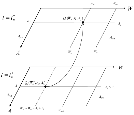
Figure 1: Illustration of the jump conditions applied on the finite difference grids.

When $W_{m}-A_{j}+A_{i}>0$, the value $Q_{t_{n}^{+}}(W_{m}-A_{j}+A_{i},r_{k},A_{i})$ can be obtained by a one-dimensional cubic spline interpolation from the values at the $M$ discrete grid points. Interpolation scheme is important, as shown for example in a convergence study by Forsyth et al. (2002), it is possible for a PDE based numerical algorithm for discretely sampled path-dependent option pricing to be non-convergent (or convergent to an incorrect answer) if the interpolation scheme is selected inappropriately.

6 Numerical Results

In this section we first show results for a benchmark test where closed-form solution exists. We then present numerical results for pricing GMWB under the static and optimal policyholder strategies using GHQC algorithm and compare these with the MC and PDE finite difference results when appropriate.

6.1 Vanilla European options

In the case of stochastic dynamics (1) for the underlying asset and interest rate, there is a closed-form solution for European vanilla options, thus providing a valuable benchmark test for numerical algorithms. In particular, the formulas for prices of vanilla call and vanilla put with strike $K_{T}$ and maturity $T$, given $S(0)$ and $r(0)$ at time $t_{0}=0$ are derived in Appendix A.5.

For this test we set the input as follows: asset volatility $\sigma_{S}=20\%$, asset spot value $S(0)=1$, interest rate spot value $r(0)=5\%$, maturity $T=1$, strike $K_{T}=0.95$, and the Vasicek interest rate model parameters $\kappa=0.0349$, $\theta=5\%$, $\sigma_{r}=1\%,\;3\%$ and $\rho=-0.2,\;0.0,\;0.2$.

We calculated the vanilla prices using the finite difference ADI method solving two-dimensional PDE (18) and our GHQC method developed in the previous sections and compared with the closed-form solution (37). Of course in the case of vanilla options, using change of numéraire to the bond $P(0,T)$, the interest rate dimensionality can be removed from numerical pricing and the required PDE can be reduced to the one-dimensional PDE similar to deterministic interest rate case. Here, we implement ADI for the original two-dimensional PDE (18) for testing and comparison purposes.

For GHQC, we used $q_{1}=12$ and $q_{2}=3$ quadrature, i.e. the total number of quadrature points for each integration is 36. The mesh for GHQC calculations was fixed at $M=100$ for $X$ dimension and $K=20$ for the interest rate $r$ dimension, and the total number of time steps $N=5$. Comparing with typical finite difference calculations, the above mesh and time steps are quite coarse. Indeed, for ADI calculations, in order to have a roughly compatible accuracy with GHQC, we had to set $M=200$, $K=40$ and $N=300$. Table 1 and Table 2 show results for vanilla call and put prices for different values of $\sigma_{r}$ and $\rho$. The percentage numbers in the parentheses in both tables are the relative numerical errors of the price compared with the closed-form solution. On average, for $\sigma_{r}=1\%$ the relative error is about $0.033\%$ for ADI and $0.042\%$ for GHQC, while for $\sigma_{r}=3\%$ the relative error is about $0.077\%$ for ADI and $0.040\%$ for GHQC. Significantly, the average relative error for ADI is more than doubled when the volatility of interest rate is increased from $\sigma_{r}=1\%$ to $\sigma_{r}=3\%$, while the error for GHQC remains more or less the same.

Table 1: Vanilla call option price for different values of $\sigma_{r}$ and $\rho$. The other input parameters are $\sigma=20\%$, $S(0)=1.0$, $r(0)=5\%$, $T=1.0$, $K_{T}=0.95$, $\kappa=0.0349$ and $\theta=5\%$.

$\sigma_{r}$	$\rho$	Closed-form	ADI	GHQC
0.01	-0.2	0.119063	0.119096 ($0.027\%$)	0.119035 ($0.024\%$)
0.01	0.0	0.119404	0.119461 ($0.027\%$)	0.119392 ($0.010\%$)
0.01	0.2	0.119743	0.119775 ($0.026\%$)	0.119700 ($0.036\%$)
0.03	-0.2	0.118531	0.118604 ($0.062\%$)	0.118528 ($0.003\%$)
0.03	0.0	0.119554	0.119626 ($0.060\%$)	0.119512 ($0.035\%$)
0.03	0.2	0.120565	0.120634 ($0.057\%$)	0.120525 ($0.033\%$)

Table 2: Vanilla put option price for different values of $\sigma_{r}$ and $\rho$. The other input parameters are $\sigma=20\%$, $S(0)=1.0$, $r(0)=5\%$, $T=1.0$, $K_{T}=0.95$, $\kappa=0.0349$ and $\theta=5\%$.

$\sigma_{r}$	$\rho$	Closed-form	ADI	GHQC
0.01	-0.2	0.042547	0.042565 ($0.041\%$)	0.042522 ($0.059\%$)
0.01	0.0	0.042888	0.042905 ($0.039\%$)	0.042878 ($0.024\%$)
0.01	0.2	0.043227	0.043243 ($0.037\%$)	0.043187 ($0.093\%$)
0.03	-0.2	0.042132	0.042175 ($0.101\%$)	0.042133 ($0.002\%$)
0.03	0.0	0.043156	0.043197 ($0.095\%$)	0.043117 ($0.091\%$)
0.03	0.2	0.044167	0.044205 ($0.087\%$)	0.044133 ($0.077\%$)

Both ADI and GHQC took a fraction of a second CPU to calculate one of the options in Table 1 and Table 2. Averaging over 200 calculations for call and put options with the same inputs as given above, we found the CPU time for each call or put calculation is 0.055 second for ADI and 0.011 second for GHQC, i.e. GHQC is about five times faster than ADI in these tests. All the calculations shown in this study were performed on a desktop with an Intel Core i5-4590 CPU@3.30GHz with a 4.00GB RAM.

It is worth commenting that for the vanilla call and put options the final payoff function is only piecewise linear, i.e. it is not a polynomial function and it is not smooth at the strike $K_{T}$ (first derivative discontinuous at $W=K_{T}$). If we apply the Gauss-Hermite quadrature only to the half domain ($W\geq K_{T}$ for call and $W\leq K_{T}$ for put), then the payoff function at the maturity is a simple linear function needing no interpolation anywhere and we found the GHQC calculations can be made as accurate as desired, virtually limited only by the machine accuracy. In the above tests we did not take advantage of this specific feature because it is not generally applicable.

6.2 GMWB pricing results

In the case of the static policyholder behavior, the withdrawal amounts are predetermined at the beginning of the contract. In this case the paths of the wealth account $W(t)$ can be simulated and a standard MC simulation method can be used to calculate the price of VA contract with GMWB. Below we show results for both static and optimal withdrawal cases. The static case allows a comparison between MC and GHQC, further validating the new algorithm. We have also implemented an efficient finite difference ADI algorithm for pricing of VA with GMWB under the static policyholder behavior solving corresponding two-dimensional PDE. In what follows, results from the GHQC method will be compared with the MC and ADI methods when applicable.

6.2.1 GMWB with static policyholder behavior

In a static case the withdrawal amount is pre-determined for each withdrawal date. In this case at each payment date the jump condition applies to the single solution (therefore no need for a grid in the guarantee account $A$ dimension). Since the withdrawal amount is known at every payment date, the stochastic paths of the underlying $W$ can be simulated by MC method. Here we compare GHQC results with those of MC and ADI methods.

Table 3 shows the prices of the VA with GMWB under the static withdrawal strategy as a function of the correlation $\rho$, comparing results between MC, ADI and GHQC. The model input parameters are $\sigma_{S}=20\%$, $\sigma_{r}=2\%$, $S(0)=W(0)=1.0$, $r(0)=5\%$, $g=10\%$, $T=1/g=10.0$, $N_{w}=4$ (quarterly withdraw frequency), $\alpha=0.006$, $\kappa=0.0349$ and $\theta=5\%$. In Peng et al. (2012), results for static GMWB pricing using similar parameters were presented for the lower and upper bound estimates of the price comparing with the MC simulation results. However, those results are for a continuous in time withdrawal case, while our results are for the discrete in time withdrawals at a quarterly frequency.

For the MC method, we have used one million sample paths simulated from the closed-form transition density under the new measure $\widetilde{\mathbb{Q}}$, so that there is no time discretization error. For both ADI and GHQC we have used two meshes, one coarser and one finer, with the finer mesh doubles the number of node points in both $r$ and $X$ dimensions. Let $M_{A}$ denote the coarser mesh for ADI with $M=200$ for $X$ dimension, $K=50$ for $r$ dimension, and $M_{A}^{\star}$ denote finer mesh for ADI with $M=400$ and $K=100$. In addition, the number of time steps for each period (between consecutive withdrawal dates) was set $N_{\Delta t}=100$ for ADI when using the coarser mesh, and it was doubled to $N_{\Delta t}=200$ when using the finer mesh $M_{A}^{\star}$. For GHQC, the coarser mesh, denoted as $M_{G}$, has $M=50$ and $K=30$, and the finer mesh for GHQC, denoted as $M_{G}^{\star}$, has $M=100$ and $K=60$. For both $M_{G}$ and $M_{G}^{\star}$ meshes, we have used a single time step between withdrawal dates, i.e. $N_{\Delta t}=1$. For the quadrature points, we used $q_{1}=5$ and $q_{2}=3$ for the coarser mesh, and $q_{1}=9$ and $q_{2}=5$ for the finer mesh. Note the finer mesh $M_{G}^{\star}$ for GHQC is overall much coarser than the coarser mesh $M_{A}$ for ADI. Comparing with typical finite difference PDE calculations required for pricing financial derivatives, the finer mesh $M_{G}^{\star}$ is actually very coarse.

In Table 3, the numbers in the parentheses next to the MC results are the standard errors due to the finite number of simulations, while for ADI and GHQC the numbers in the parentheses are the relative difference from MC results. On average, the relative standard error for MC (standard error divided by the estimated mean) is 4.6E-4, sufficiently small for the MC results to serve as a basis to compare among different results.

If a set of numerical results have the same or better accuracy than the MC results, then the relative difference between this set of results and MC results should be in the same order of magnitude as the relative standard error of the MC. Results in Table 3 show that, the average relative difference between ADI and MC is about 9.2E-4 for the coarser mesh $M_{A}$, and it is about 6.9E-4 for the finer mesh $M_{A}^{\star}$. In comparison, the average relative difference between GHQC and MC is about 5.6E-4 for the coarser mesh $M_{G}$, and it is about 3.7E-4 for the finer mesh $M_{G}^{\star}$. These relative differences are indicative that the GHQC calculations are perhaps more accurate than the ADI, even comparing GHQC results of coarser mesh $M_{G}$ with ADI results of the finer mesh $M_{A}^{\star}$.

Table 3: Price of VA with GMWB under static withdrawal strategy for different values $\rho$. Other parameters: $\sigma=20\%$, $\sigma_{r}=2\%$, $S(0)=1.0$, $r(0)=5\%$, $g=10\%$ ($T=1/g$), $N_{w}=4$, $\alpha=0.006$, $\kappa=0.0349$, $\theta=5\%$.

$\rho$	MC	ADI ($M_{A}$)	ADI ($M_{A}^{\star}$)	GHQC ($M_{G}$)	GHQC ($M_{G}^{\star}$)
-0.6	1.004826 (3.1E-4)	1.00616 (1.3E-3)	1.00532 (4.9E-4)	1.00557 (7.4E-4)	1.00484 (1.4E-5)
-0.4	1.011952 (4.5E-4)	1.01338 (1.4E-3)	1.01255 (5.9E-4)	1.01295 (9.8E-4)	1.01236 (4.0E-4)
-0.2	1.019002 (4.8E-4)	1.02024 (1.2E-3)	1.01942 (4.1E-4)	1.01982 (8.0E-4)	1.01945 (4.4E-4)
0.0	1.026177 (4.8E-4)	1.02675 (5.6E-4)	1.02592 (2.5E-4)	1.02625 (7.9E-5)	1.02613 (4.6E-5)
0.2	1.032256 (4.8E-4)	1.03289 (6.1E-4)	1.03206 (1.9E-4)	1.03279 (5.2E-4)	1.03249 (2.3E-4)
0.4	1.038966 (5.3E-4)	1.03867 (2.8E-4)	1.03784 (1.1E-3)	1.03886 (1.0E-4)	1.03849 (4.6E-4)
0.6	1.045171 (5.8E-4)	1.04407 (1.1E-3)	1.04325 (1.8E-3)	1.04445 (6.9E-4)	1.04413 (9.9E-4)

Not only the GHQC may have better accuracy than the ADI, the CPU time comparison is even more impressive: for ADI calculations, the CPU time per price is 1.0 second and 7.6 second for the coarser and finer mesh, respectively; while for GHQC calculations, the CPU time per price is 0.02 second and 0.24 second for the coarser and finer mesh, respectively. In other words, comparing the coarser mesh calculations, the GHQC is about 50 times as fast as ADI, and comparing the finer mesh calculations the GHQC is about 30 times as fast as ADI, while achieving better accuracy. Only the GHQC results with the finer mesh has an average relative difference (relative to MC results) smaller than the average relative standard error of MC with one million simulations.

Table 4: Prices of VA with GMWB under static withdrawal strategy for different fees $\alpha$ and positive correlation $\rho=0.3$. Other parameters: $\sigma=20\%$, $\sigma_{r}=2\%$, $S(0)=1.0$, $r(0)=5\%$, $g=10\%$ (i.e. $T=1/g$), $N_{w}=4$, $\kappa=0.0349$ and $\theta=5\%$.

$\alpha$	MC	ADI ($M_{A}^{\star}$)	GHQC ($M_{G}^{\star}$)
0	1.064589 (5.2E-4)	1.06389 (6.6E-4)	1.06434 (2.3E-4)
25	1.052354 (5.0E-4)	1.05154 (7.7E-4)	1.05202 (3.2E-4)
50	1.040172 (4.9E-4)	1.03963 (5.2E-4)	1.04015 (2.2E-5)
75	1.029112 (4.9E-4)	1.02817 (9.2E-4)	1.02873 (3.7E-4)
100	1.018198 (4.7E-4)	1.01714 (1.0E-3)	1.01773 (4.6E-4)
125	1.007269 (4.7E-4)	1.00653 (7.3E-4)	1.00716 (1.1E-4)
150	0.997382 (4.5E-4)	0.996316 (1.1E-3)	0.996993 (3.9E-4)
175	0.987463 (4.4E-4)	0.986501 (9.7E-4)	0.987222 (2.4E-4)
200	0.977950 (4.3E-4)	0.977069 (9.0E-4)	0.977835 (1.2E-4)

Table 5: Prices of VA with GMWB under static withdrawal strategy for different fees $\alpha$ and negative correlation $\rho=-0.3$. Other parameters: $\sigma=20\%$, $\sigma_{r}=2\%$, $S(0)=1.0$, $r(0)=5\%$, $g=10\%$ (i.e. $T=1/g$), $N_{w}=4$, $\kappa=0.0349$ and $\theta=5\%$.

$\alpha$	MC	ADI ($M_{A}^{\star}$)	GHQC ($M_{G}^{\star}$)
0	1.044794 (5.3E-4)	1.04526 (4.5E-4)	1.04495 (1.5E-4)
25	1.032550 (5.1E-4)	1.03274 (1.8E-4)	1.03253 (2.0E-5)
50	1.020225 (5.0E-4)	1.02071 (4.7E-4)	1.02059 (3.6E-4)
75	1.009109 (5.0E-4)	1.00915 (4.1E-5)	1.00912 (1.1E-5)
100	0.9978363 (4.8E-4)	0.998039 (2.0E-4)	0.998104 (2.7E-4)
125	0.9871583 (4.8E-4)	0.987377 (2.2E-4)	0.987531 (3.8E-4)
150	0.9770732 (4.6E-4)	0.977148 (7.7E-5)	0.977387 (3.2E-4)
175	0.9673112 (4.4E-4)	0.967338 (2.8E-5)	0.967662 (3.6E-4)
200	0.9581683 (4.4E-4)	0.957938 (2.4E-4)	0.958343 (1.8E-4)

Table 4 shows the price of the VA with GMWB under the static withdrawal strategy as a function of the fee $\alpha$ in the unit of basis point (a basis point is 0.01% ). The correlation $\rho$ is fixed at $\rho=0.3$ and all the other inputs are the same as for the calculations for Table 3. For ADI and GHQC, only results of the finer meshes $M_{A}^{\star}$ and $M_{G}^{\star}$ are shown. The number of simulations for MC and the number of time steps for ADI and GHQC were unchanged. In this case the average relative standard error for MC is 4.7E-4. The average relative difference between ADI and MC is 8.4E-4, somewhat larger than the MC standard error. The average relative difference between GHQC and MC is 2.5E-4, which is about half of the MC standard error.

Table 5 shows the same results as Table 4 except the correlation is negative at $\rho=-0.3$. In this case the average relative standard error for MC is 4.8E-4. The average relative difference between ADI and MC is 2.1E-4, and the average relative difference between GHQC and MC is 2.3E-4, both are about half of the MC standard error.

It is interesting to compare the results of Vasicek model with the case of deterministic interest rate set to be $r(0)$ during the contract life. We found that, for the test cases shown in Table 4 where the correlation is positive at $\rho=0.3$, the static withdrawal strategy GMWB prices under the stochastic interest rate are about $2\%$ larger than the deterministic counterpart, i.e. the ratio in prices is about $1.02$. However, a small difference in the price for a given fee does not not mean a small difference in the fair fees given the premium. A fair fee $\alpha$ is the fee making the initial premium equal to the contract price, i.e. $Q(W(0),r(0),W(0))=W(0)$. For the inputs given for Table 4, we found the fair fee for GMWB under the stochastic interest rate is 143 basis points, which is $49\%$ higher than the deterministic case of 95.8 basis points.

On the other hand, for the cases in Table 5 where the correlation is negative at $\rho=-0.3$, the prices of VA with the static withdrawal GMWB under the stochastic interest rate are virtually the same as the deterministic interest rate counterpart – on average the relative difference in prices is about 3.5E-4, which has the same magnitude as the average relative errors. The corresponding relative difference in the fair fees of GMWB between the stochastic interest rate and deterministic rate cases is only about $0.2\%$, which could be in the same order of magnitude as numerical errors in the fees.

6.2.2 GMWB under optimal withdrawals

Having numerically validated the implementation of GHQC algorithm, we then proceed to perform calculations for pricing of GMWB under the dynamic withdrawal strategy. Note that for the dynamic strategy GMWB pricing, exactly the same numerical functions are used as for the static strategy GMWB case. The only extra step required for the dynamic case is simply finding the optimal amount among possible withdrawal values, while in the static case only the fixed withdrawal amount is considered. In particular, the integration and jump condition application all use identical functions in the dynamic and static cases.

Table 6 is the dynamic strategy counterpart of Table 4, i.e. all the inputs (model parameters, contract details, mesh, quadrature points and time step settings) are the same, but the calculations are for the dynamic withdrawals. In this example the number of grid points in the guarantee account $A$ is $J=100$. An extra input needed for the dynamic case is the penalty coefficient $\beta$, which is fixed at $\beta=10\%$ in all the following calculations. A simple extra validation for the dynamic calculations is to set the penalty coefficient $\beta$ very high, say $\beta=50\%$, then the price under the optimal withdrawals should be the same as under the static withdrawals, which was indeed confirmed by our numerical tests.

Table 6: Prices of VA with GMWB under dynamic withdrawal strategy for different fees $\alpha$ in the case of negative and positive correlation $\rho$. Other parameters: $\sigma_{S}=20\%$, $\sigma_{r}=2\%$, $S(0)=1.0$, $r(0)=5\%$, $g=10\%$ ($T=1/g$), $\beta=10\%$, $N_{w}=4$, $\kappa=0.0349$, $\theta=5\%$.

$\alpha$	GHQC ($\rho=-0.3$)	GHQC ($\rho=0.3$)
0	1.08348	1.10173
25	1.06651	1.08367
50	1.05107	1.06707
75	1.03719	1.05184
100	1.02484	1.03804
125	1.01389	1.02558
150	1.00408	1.01446
175	0.995356	1.00463
200	0.987673	0.996057

We also show comparison of the prices for the cases of deterministic and stochastic interest rates in Figure 2. Similar to the static withdrawal case, with a positive correlation between asset and interest rate $\rho=0.3$, prices of the VA with dynamic withdrawal GMWB under the stochastic interest rate are about $2\%$ larger than in the case of deterministic constant interest rate set to $r(0)$, i.e. the ratio in prices is about $1.02$. Again, a small difference in the price for a given fee does not not mean a small difference in the fair fees given the premium. For the inputs given for Table 6, we found the fair fee for GMWB under the stochastic interest rate is 188 basis points, which is $38\%$ higher than the fair fee 136 basis points in the case of deterministic interest rate.

Similar to the static withdrawal case, in the case of negative correlation between asset and interest rate $\rho=-0.3$, the differences of prices between cases under the stochastic interest rate and cases under a deterministic interest rate $r(0)$ are relatively small, compared with the case of positive correlation. Now, at $\rho=-0.3$, these differences are only about $0.9\%$ on average, much smaller than $2\%$ when the correlation is at $\rho=0.3$. However, unlike the static withdrawal case where for $\rho=-0.3$ the difference of prices between stochastic rate and deterministic rate is negligible (as small as the numerical errors), the difference of $0.9\%$ is still significant (the estimated relative numerical error is in the order of $0.01\%$), leading to a significant difference in the fair fees. We found for this case at $\rho=-0.3$, the fair fee under the stochastic rate is 161 basis points, which is about $19\%$ higher than the deterministic interest rate counterpart (136 basis points).

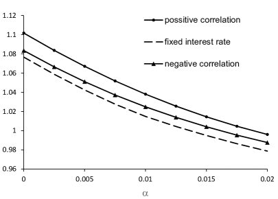
Figure 2: Prices of VA with GMWB under optimal withdrawals and stochastic interest rate with $\rho=0.3$ and $\rho=-0.3$. The other parameters are the same as for Table 6.

As expected, the CPU time for these calculations of dynamic withdrawal cases is much longer than the static withdrawal counterpart with the same mesh and time steps. The average CPU time for calculating the prices in Table 6 is about 39 seconds per price, comparing with 0.24 second per price for the static withdrawal case with the same mesh and time steps. The ratio of these CPUs is about 160, which is reasonable because instead of tracking a single two dimensional solution in $(X,r)$ for the static withdrawal case, for the dynamic withdrawal case we have to track $J=100$ such solutions for all the nodes in $A$. In addition, on each withdrawal date all the possible jumps have to be performed in order to find the optimal withdrawal amount for each grid point in $(X,r,A)$ space, as compared to the static withdrawal case where only one jump is needed for each single grid point in $(X,r)$ space.

7 Conclusion

In this paper we developed a new direct integration method for pricing of the VA with guarantees under the both static and dynamic (optimal) policyholder behaviors in the case of stochastic interest rate. Using bond price as a numéraire, we have derived the closed-form bivariate transition density for the correlated state variables $\ln S(t)$ and $r(t)$. Under the new measure the required expectations are reduced to the two-dimensional integrals which can be readily calculated through the two-dimensional numerical integration using Gauss-Hermite quadrature, allowing an efficient backward time stepping for solving recursive Bellman equation. A spectral rotation scheme preserves the symmetry with respect to the principal axes of the bivariate random field, yielding a robust and accurate quadrature application. A two-dimensional cubic spline interpolation on the finite grids for $(X(t),r(t))$ is utilized to provide the continuous function required by the quadratures. The proper jump conditions are applied at each withdrawal date that allows the optimal withdrawal decision to be made.

The algorithm is convincingly validated by comparing to the European option pricing where closed-form analytical solution exists, and by static withdrawal GMWB pricing where MC and PDE ADI methods can provide good benchmark solutions. Numerical tests show the accuracy of the presented GHQC method is at least compatible to a typical ADI finite difference scheme, but it is more robust and significantly faster.

For dynamic withdrawal GMWB pricing, using the new algorithm we found some interesting results which we believe are new to the literature. When the correlation between the underlying risky asset and interest rate is positive, the GMWB price or equivalently the fee under the stochastic interest rate is significantly higher than in the case of deterministic interest rate. In the particular test problem, the fee in the case of stochastic interest rate is about $40\%$ higher than the deterministic case when $\rho=0.3$. When the correlation is negative, the differences are still significant but much less than in the case of positive correlation. The fee in the case of stochastic interest rate is about $20\%$ higher than the deterministic case when correlation is negative at $\rho=-0.3$. On the other hand, the situation in the static withdrawal pricing is remarkably different: at negative correlation, the differences in prices and fees of GMWB between stochastic and deterministic settings are virtually negligible.

In this paper we focused on pricing of a very basic GMWB structure. However, presented algorithm can be easily adapted to pricing other VA guarantees and solving similar stochastic control problems with two state variables possibly affected by control. Applications to pricing Asian, barrier and other financial derivatives with a single underlying risky and stochastic interest rate are straightforward. Also, it should be possible to extend the algorithm to situations when the underlying bivariate transition density is not known in closed-form but its moments are known, similarly as developed in Luo and Shevchenko (2014) for one-dimensional problems; this is a subject of future research.

8 Acknowledgement

This research was supported by the CSIRO-Monash Superannuation Research Cluster, a collaboration among CSIRO, Monash University, Griffith University, the University of Western Australia, the University of Warwick, and stakeholders of the retirement system in the interest of better outcomes for all. This research was also partially supported under the Australian Research Council’s Discovery Projects funding scheme (project number: DP160103489).

Appendix A Joint Distribution of $S(t)$, $r(t)$ and $Y(t)=\int_{0}^{t}r(u)du$

Consider the probability measure $\mathbb{Q}$ with corresponding stochastic processes for $S(t)$ and $r(t)$ given by (1), and the new probability measure $\widetilde{\mathbb{Q}}$ obtained via the Radon-Nikodym derivative

$$\mathbb{Z}_{t}=\left.\frac{d\widetilde{\mathbb{Q}}}{d\mathbb{Q}}\right|_{\mathcal{F}_{t}}=\frac{M(0)}{M(t)}\frac{P(t,T)}{P(0,T)},\quad t\in[0,T].$$ (30)

Here, $M(t)=e^{\int_{0}^{t}r(\tau)d\tau}$ is the money market account and $P(t,T)=\mathrm{E}^{\mathbb{Q}}_{0}[e^{-\int_{t}^{T}r(\tau)d\tau}]$ is the $T$-maturity bond. In particular, it is easy to see that $\mathbb{Z}_{T}>0$ and $\mathrm{E}_{0}^{\mathbb{Q}}[\mathbb{Z}_{T}]=1$ and this change of measure leads to the following formula for an arbitrary function $f(S(T),r(T))$

$$\mathrm{E}^{\mathbb{Q}}_{0}\left[e^{-\int_{0}^{T}r(u)du}f(S(T),r(T))\right]=P(0,T){\mathrm{E}}^{\widetilde{\mathbb{Q}}}_{0}\left[f(S(T),r(T)\right],$$

assuming that these expectations exist. One can say that we changed numéraire from the money market account $M(t)$ to the $T$-maturity bond $P(t,T)$. Using Itô’s formula, the process for $\mathbb{Z}_{t}$ is easily obtained from the process (3) for the bond price $P(t,T)$ to be

$$d\mathbb{Z}_{t}=\phi(t)\mathbb{Z}_{t}d\mathcal{B}_{1},\quad\phi(t)=-\sigma_{r}B_{t,T},$$

where $B_{t,T}=(1-e^{-\kappa(T-t)})/\kappa$, and Girsanov theorem gives the corresponding transformation to the Wiener process $\mathcal{B}_{1}(t)=\phi(t)dt+d\widetilde{\mathcal{B}}_{1}(t)$. Thus the processes for $S(t)$ and $r(t)$ under the new measure $\widetilde{\mathbb{Q}}$ for $t\in[0,T]$ are

$$\begin{split}dS(t)/S(t)&=(r(t)+\sigma_{S}\rho\phi(t))dt+\sigma_{S}\left(\rho d\widetilde{\mathcal{B}}_{1}(t)+\sqrt{1-\rho^{2}}d\widetilde{\mathcal{B}}_{2}(t)\right),\\ dr(t)&=\kappa\left(\widetilde{\theta}(t)-r(t)\right)dt+\sigma_{r}d\widetilde{\mathcal{B}}_{1}(t);\;\widetilde{\theta}(t)=\theta+\frac{\sigma_{r}}{\kappa}\phi(t)\end{split}$$ (31)

with $\widetilde{\mathcal{B}}_{1}(t)$ and $\widetilde{\mathcal{B}}_{2}(t)$ independent Wiener processes.

In this section we derive the joint Normal distribution of $\ln S(t)$ and $r(t)$ for given $S(0)$ and $r(0)$ under the new probability measure $\widetilde{\mathbb{Q}}$. We also derive the bond price, European vanilla price formulas, and 3d joint Normal distribution of $\ln S(t)$, $r(t)$ and $Y(t)=\int_{0}^{t}r(u)du$ conditional on $S(0)$ and $r(0)$ under the measure $\mathbb{Q}$. The last is useful for validation tests to simulate and calculate the contract payoff without time discretization error. Some of these formulas can be found in the literature, e.g. see (Cairns, 2004, appendix B1 and section 4.5) for bond price and distribution of $(r(t),Y(t))$ under the Vasicek model, but are presented here for completeness and notational consistency.

The formulas derived below for the mean and covariances can be used for simulation of $(S({t_{n}}),r({t_{n}}))$ given $(S({t_{n-1}}),r({t_{n-1}}))$. One has to just set $t\rightarrow t_{n}-t_{n-1}$, $T\rightarrow T-t_{n-1}$, and $r(t_{0})\rightarrow r({t_{n-1}})$, $S(0)\rightarrow S({t_{n-1}})$ in these formulas. To obtain the mean and covariance formulas (19) required to calculate expectation (15) over $(t_{n-1},t_{n})$ one has to set $t=T\rightarrow t_{n}-t_{n-1}$ and subtract $\alpha\times(t_{n}-t_{n-1})$ from the mean of $\ln S(t_{n})$ to get the mean of $\ln W(t_{n})$.

A.1 Distribution for $r(t)$

The solution for the interest rate $r(t)$ given $r(0)$, with the process in (16) under $\widetilde{\mathbb{Q}}$, is

$$r(t)=r(0)e^{-\kappa t}+e^{-\kappa t}\kappa\int_{0}^{t}\widetilde{\theta}(\tau)e^{\kappa\tau}d\tau+\sigma_{r}e^{-\kappa t}\int_{0}^{t}e^{\kappa\tau}d\widetilde{\mathcal{B}}_{1}(\tau)$$ (32)

that can be checked directly by denoting $H_{t}=\int_{0}^{t}e^{\kappa\tau}d\widetilde{\mathcal{B}}_{1}(\tau)$, $r(t):=g(t,H_{t})$ and then calculating $dr(t)=dg(t,H_{t})$ using Itô formula to obtain the process $dr(t)$ in (16). Thus, $r(t)$ conditional on $r(0)$ is from Normal distribution with

$$\begin{split}\mu_{r}(t):=\mathrm{mean}(r(t))&=r(0)e^{-\kappa t}+e^{-\kappa t}\kappa\int_{0}^{t}\widetilde{\theta}(\tau)e^{\kappa\tau}d\tau,\\ \mathrm{var}(r(t))&=\frac{\sigma_{r}^{2}}{2\kappa}\left(1-e^{-2\kappa t}\right).\end{split}$$ (33)

In the case of constant in time parameter $\theta$, simple integration yields

$$\mu_{r}(t)=r(0)e^{-\kappa t}+\theta\left(1-e^{-\kappa t}\right)+\frac{\sigma_{r}^{2}}{2\kappa^{2}}\left((1-e^{-2\kappa t})e^{-\kappa(T-t)}-2(1-e^{-\kappa t})\right).$$

In the case of risk-neutral process (1) under the measure $\mathbb{Q}$, the last term with factor ${\sigma_{r}^{2}}$ in the above formula for $\mu_{r}(t)$ should be set to zero and no change to the variance is required.

A.2 Distribution for $Y(t)=\int_{0}^{t}r(u)du$

Using solution (32) for $r(t)$, direct calculation of $Y(t)$ under the probability measure $\widetilde{\mathbb{Q}}$ gives

$$Y(t)=\int_{0}^{t}r(\tau)d\tau = \int_{0}^{t}\mu_{r}(\tau)d\tau+\sigma_{r}\int_{0}^{t}e^{-\kappa\tau}d\tau\int_{0}^{\tau}e^{\kappa s}d\widetilde{\mathcal{B}}_{1}(s)ds$$ (34)

$$= \int_{0}^{t}\mu_{r}(\tau)d\tau+\sigma_{r}\int_{0}^{t}d\widetilde{\mathcal{B}}_{1}(s)\int_{s}^{t}e^{-\kappa(\tau-s)}d\tau$$

$$= \int_{0}^{t}\mu_{r}(\tau)d\tau+\frac{\sigma_{r}}{\kappa}\int_{0}^{t}(1-e^{-\kappa(t-s)})d\widetilde{\mathcal{B}}_{1}(s),$$

where the $2d$ integral involving $\widetilde{\mathcal{B}}_{1}(t)$ was simplified by changing order of the integrations. Thus the distribution of $Y(t)$ is Normal with the mean and variance calculated via the standard integrations

$$\begin{split}I_{1}(t):=\mathrm{mean}(Y(t))&=\int_{0}^{t}\mu_{r}(\tau)d\tau,\\ \mathrm{var}(Y(t))&=\frac{\sigma_{r}^{2}}{\kappa^{2}}\int_{0}^{t}\left(1-e^{-\kappa(t-s)}\right)^{2}ds\\ &=\frac{\sigma_{r}^{2}}{\kappa^{2}}\left(t-\frac{2}{\kappa}(1-e^{-\kappa t})+\frac{1}{2\kappa}(1-e^{-2\kappa t})\right),\end{split}$$

where $I_{1}(t)$ in the case of constant in time parameter $\theta$ can be found in closed-form

$$I_{1}(t)=\frac{1}{\kappa}(1-e^{-\kappa t})\left(r_{0}-\theta+\frac{\sigma_{r}^{2}}{2\kappa^{2}}\left(2-e^{-\kappa T}+e^{-\kappa(T-t)}\right)\right)+\left(\theta-\frac{\sigma_{r}^{2}}{\kappa^{2}}\right)t.$$

In the case of the risk-neutral process (1) under the measure $\mathbb{Q}$, $\sigma_{r}$ in the above formula for $I_{1}(t)$ should be set to zero and no change to the variance is required.

A.3 Distribution for $\ln S(t)$

The solution for $\ln S(t)$ given $\ln S(0)$, with the process in (16) under $\widetilde{\mathbb{Q}}$, is given by

$$\begin{split}\ln S(t)=&\ln S(0)+\int_{0}^{t}r(\tau)d\tau+\rho\sigma_{S}\int_{0}^{t}\phi(\tau)d\tau-\frac{1}{2}\sigma_{S}^{2}t\\ &+\rho\sigma_{S}\int_{0}^{t}d\widetilde{\mathcal{B}}_{1}(\tau)+\sigma_{S}\sqrt{1-\rho^{2}}\int_{0}^{t}d\widetilde{\mathcal{B}}_{2}(\tau).\end{split}$$ (35)

Substituting (34) it is easy to see that $\ln S(t)$ is from Normal distribution and performing simple integrations obtain

$$\begin{split}\mathrm{mean}(\ln S(t))&=\ln S(0)+I_{1}(t)-\frac{1}{2}\sigma_{S}^{2}t-\frac{\rho\sigma_{S}\sigma_{r}}{\kappa^{2}}\left(\kappa t-e^{-\kappa T}(e^{\kappa t}-1)\right),\\ \mathrm{var}(\ln S(t))&=\sigma_{S}^{2}t+\frac{\sigma_{r}^{2}}{2\kappa^{3}}\left(2\kappa t-3+4e^{-\kappa t}-e^{-2\kappa t}\right)+\frac{2\rho\sigma_{S}\sigma_{r}}{\kappa^{2}}\left(\kappa t-1+e^{-\kappa t}\right).\end{split}$$

In the case of risk-neutral process (1) under the measure $\mathbb{Q}$, the last term proprotional to $\rho$ in the above formula for $\mathrm{mean}(\ln S(t))$ should be set to zero and no change to the variance is required.

A.4 Covariances between $\ln S(t)$, $r(t)$ and $Y(t)=\int_{0}^{t}r(u)du$

Direct calculations using solutions (35), (32) and (34) for $\ln S(t)$, $r(t)$ and $Y(t)$ conditional on $\ln S(0)$ and $r(0)$, under the probability measure $\widetilde{\mathbb{Q}}$, yield

$$\begin{split}\mathrm{cov}(\ln S(t),r(t))&=\sigma_{r}\int_{0}^{t}\left(\sigma_{S}\rho+\frac{\sigma_{r}}{\kappa}\left(1-e^{-\kappa(t-s)}\right)\right)e^{-\kappa(t-s)}ds\\ &=\frac{\rho\sigma_{S}\sigma_{r}}{\kappa}\left(1-e^{-\kappa t}\right)+\frac{\sigma_{r}^{2}}{2\kappa^{2}}\left(1-2e^{-\kappa t}+e^{-2\kappa t}\right),\\ \mathrm{cov}(Y(t),r(t))&=\frac{\sigma_{r}^{2}}{\kappa}e^{-\kappa t}\int_{0}^{t}e^{\kappa s}\left(1-e^{-\kappa(t-s)}\right)ds\\ &=\frac{\sigma_{r}^{2}}{2\kappa^{2}}\left(1-2e^{-\kappa t}+e^{-2\kappa t}\right),\\ \mathrm{cov}(\ln S(t),Y(t))&=\frac{\sigma_{r}}{\kappa}\int_{0}^{t}(1-e^{-\kappa(t-s)})\left(\sigma_{S}\rho+\frac{\sigma_{r}}{\kappa}\left(1-e^{-\kappa(t-s)}\right)\right)ds\\ &=\frac{\rho\sigma_{S}\sigma_{r}}{\kappa^{2}}\left(\kappa t-1+e^{-\kappa t}\right)+\frac{\sigma_{r}^{2}}{2\kappa^{3}}\left(2\kappa t-3+4e^{-\kappa t}-e^{-2\kappa t}\right).\end{split}$$

These formulas for covariances are the same in the case of the risk-neutral process (1) under the probability measure $\mathbb{Q}$.

A.5 Bond and Vanilla prices

Zero coupon bond price $P(t,T)=\mathrm{E}_{t}^{\mathbb{Q}}\left[e^{-\int_{t}^{T}r(u)du}\right]$ in the case of Vasicek interest rate model (1) can be calculated directly using distribution of random variable $Y=\int_{t}^{T}r(u)du$ which is Normal with the mean and variance derived in Appendix A.2. This gives

$$\begin{split}P(t,T)&=e^{-\mathrm{mean}(Y)+\frac{1}{2}\mathrm{var}(Y)}=e^{A_{t,T}-r(t)B_{t,T}},\\ B_{t,T}&=\frac{1}{\kappa}\left(1-e^{-\kappa(T-t)}\right),\\ A_{t,T}&=-\kappa\int_{t}^{T}\theta B_{s,T}ds+\frac{\sigma_{r}^{2}}{4\kappa^{3}}\left(2\kappa(T-t)+4e^{-\kappa(T-t)}-e^{-2\kappa(T-t)}-3\right).\end{split}$$ (36)

Allowing $\theta:=\theta(t)$ to be time dependent parameter, one can find $\theta(t)$ yielding bond prices observed at $t=0$. In the case of constant $\theta$, the above formula for $A_{t,T}$ simplifies to

$$A_{t,T}=\left(\theta-\frac{\sigma_{r}^{2}}{2\kappa^{2}}\right)\left(B_{t,T}-(T-t)\right)-\frac{\sigma_{r}^{2}}{4\kappa}B_{t,T}^{2}.$$

In the case of the risk-neutral process (1) for $S(t)$ and $r(t)$ under the measure ${\mathbb{Q}}$, the closed-form formulas for prices of vanilla call $Q_{t_{0}}^{\mathrm{call}}$ and vanilla put $Q_{t_{0}}^{\mathrm{put}}$ with strike $K_{T}$ at maturity $T$, given $S(0)$ and $r(0)$, at time $t_{0}=0$ can be easily found. Changing measure ${\mathbb{Q}}$ to $\widetilde{\mathbb{Q}}$ and using formulas for the mean and variance of Normally distributed $\ln S(T)$ under $\widetilde{\mathbb{Q}}$ derived in Appendix A.3, obtain after simple calculus

$$\begin{split}Q_{t_{0}}^{\mathrm{call}}&=\mathrm{E}_{t_{0}}^{\mathbb{Q}}\left[e^{-\int_{0}^{T}r(u)du}\max(S(T)-K_{T},0)\right]\\ &=P(0,T)\mathrm{E}_{t_{0}}^{\widetilde{\mathbb{Q}}}\left[\max(S(T)-K_{T},0)\right]\\ &=S(0)N(d_{1})-K_{T}P(0,T)N(d_{2}),\\ Q_{t_{0}}^{\mathrm{put}}&=\mathrm{E}_{t_{0}}^{\mathbb{Q}}\left[e^{-\int_{0}^{T}r(u)du}\max(S(T)-K_{T},0)\right]\\ &=P(0,T)\mathrm{E}_{t_{0}}^{\widetilde{\mathbb{Q}}}\left[\max(S(T)-K_{T},0)\right]\\ &=K_{T}P(0,T)N(-d_{2})-S(0)N(-d_{1}).\end{split}$$ (37)

Here, $N(x)$ is the standard Normal distribution function, $P(0,T)$ is the bond price given by (2), $d_{1}=(\ln({S(0)}/{K_{T}})-\ln P(0,T)+\frac{1}{2}\sigma^{2}_{\mathrm{eff}})/\sigma_{\mathrm{eff}}$, $d_{2}=d_{1}-\sigma_{\mathrm{eff}}$ and

$$\sigma^{2}_{\mathrm{eff}}=\sigma_{S}^{2}T+\frac{\sigma_{r}^{2}}{2\kappa^{3}}\left(2\kappa T-3+4e^{-\kappa T}-e^{-2\kappa T}\right)+\frac{2\rho\sigma_{S}\sigma_{r}}{\kappa^{2}}\left(\kappa T-1+e^{-\kappa T}\right).$$ (38)

Note, the derived formulas are the same as the well known Black-Scholes formulas for call and put under the constant interest rate $r$ and volatility $\sigma$ if $rT$ is replaced by $-\ln P(0,T)$ and $\sigma^{2}T$ is replaced by $\sigma^{2}_{\mathrm{eff}}$.

References

- Azimzadeh and Forsyth (2014) Azimzadeh, Y. and P. A. Forsyth (2014). The existence of optimal bang-bang controls for GMXB contracts. Working paper of University of Waterloo.
- Bacinello et al. (2011) Bacinello, A., P. Millossovich, A. Olivieri, and E. Pitacco (2011). Variable annuities: a unifying valuation approach. Insurance: Mathematics and Economics 49(1), 285–297.
- Bauer et al. (2008) Bauer, D., A. Kling, and J. Russ (2008). A universal pricing framework for guaranteed minimum benefits in variable annuities. ASTIN Bulletin 38(2), 621–651.
- Bäuerle and Rieder (2011) Bäuerle, N. and U. Rieder (2011). Markov Decision Processes with Applications to Finance. Springer, Berlin.
- Björk (2009) Björk, T. (2009). Arbitrage Theory in Continuous Time (3rd ed.). Oxford University Press.
- Cairns (2004) Cairns, A. (2004). Interest Rate Models: An Introduction. New Jersey: Princeton University Press.
- Chen and Forsyth (2008) Chen, Z. and P. Forsyth (2008). A numerical scheme for the impulse control formulation for pricing variable annuities with a guaranteed minimum withdrawal benefit (GMWB). Numerische Mathematik 109(4), 535–569.
- Dai et al. (2008) Dai, M., Y. K. Kwok, and J. Zong (2008). Guaranteed minimum withdrawal benefit in variable annuities. Mathematical Finance 18(4), 595–611.
- Forsyth and Vetzal (2014) Forsyth, P. and K. Vetzal (2014). An optimal stochastic control framework for determining the cost of hedging of variable annuities. Journal of Economic Dynamics & Control 44, 29–53.
- Forsyth et al. (2002) Forsyth, P. A., K. R. Vetzal, and R. Zvan (2002). Convergence of numerical methods for valuing path-dependent options using interpolation. Review of Derivatives Research 5, 273–314.
- Gordon (1965) Gordon, P. (1965). Nonsymmetric difference equations. Journal of the Society for Industrial and Applied Mathematics 13, 667–673.
- Gourlay (1970) Gourlay, A. R. (1970). Hopscotch: a fast second-order partial differential equation solver. IMA Journal of Applied Mathematics 6(4), 375–390.
- Gourlay and McKee (1977) Gourlay, A. R. and S. McKee (1977). The construction of hopscotch methods for parabolic and elliptic equations in two space dimensions with a mixed derivative. Journal of Computational and Applied Mathematics 3(3), 201–206.
- Huang and Forsyth (2012) Huang, Y. and P. A. Forsyth (2012). Analysis of a penalty method for pricing a guaranteed minimum withdrawal benefit (GMWB). Journal of Numerical Analysis 32, 320–351.
- Huang and Kwok (2014) Huang, Y. and Y. K. Kwok (2014). Analysis of optimal dynamic withdrawal policies in withdrawal guarantee products. Journal of Economic Dynamics and Control 45, 19–43.
- Huang and Kwok (2015) Huang, Y. and Y. K. Kwok (2015). Regression-based Monte Carlo methods for stochastic control models: variable annuities with lifelong guarantees. Working Paper.
- Kalberer and Ravindran (2009) Kalberer, T. and K. Ravindran (2009). Variable Annuities: a global perspective. London: Risk Books.
- Kharroubi et al. (2014) Kharroubi, I., N. Langrené, and H. Pham (2014). A numerical algorithm for fully nonlinear HJB equations: an approach by control randomization. Monte Carlo Methods and Applications 20(2), 145––165.
- Ledlie et al. (2008) Ledlie, M., D. Corry, G. Finkelstein, A. Ritchie, K. Su, and D. Wilson (2008). Variable annuities. British Actuarial Journal 14(Part II 61), 327 –389.
- Longstaff and Schwartz (2001) Longstaff, F. and E. Schwartz (2001). Valuing American options by simulation: a simple least-squares approach. Review of Financial Studies 14, 113–147.
- Luo and Shevchenko (2014) Luo, X. and P. V. Shevchenko (2014). Fast and simple method for pricing exotic options using Gauss-Hermite quadrature on a cubic spline interpolation. Journal of Financial Engineering 1(4), 1450033. DOI: 10.1142/S2345768614500330.
- Luo and Shevchenko (2015a) Luo, X. and P. V. Shevchenko (2015a). Fast numerical method for pricing of variable annuities with guaranteed minimum withdrawal benefit under optimal withdrawal strategy. International Journal of Financial Engineering 2(3), 1550024. DOI: 10.1142/S2424786315500243.
- Luo and Shevchenko (2015b) Luo, X. and P. V. Shevchenko (2015b). Valuation of variable annuities with guaranteed minimum withdrawal and death benefits via stochastic control optimization. Insurance: Mathematics and Economics 62, 5–15. DOI: 10.1016/j.insmatheco.2015.02.003.
- Luo and Shevchenko (2015c) Luo, X. and P. V. Shevchenko (2015c, December). Variable annuity with GMWB: surrender or not, that is the question. In T. Weber, M. J. McPhee, and R. S. Anderssen (Eds.), MODSIM2015, 21st International Congress on Modelling and Simulation. Modelling and Simulation Society of Australia and New Zealand, pp. 959–965. ISBN: 978-0-9872143-5-5, http://www.mssanz.org.au/modsim2015/E1/luo.pdf.
- Milevsky and Salisbury (2006) Milevsky, M. A. and T. S. Salisbury (2006). Financial valuation of guaranteed minimum withdrawal benefits. Insurance: Mathematics and Economics 38(1), 21–38.
- Moenig and Bauer (2015) Moenig, T. and D. Bauer (2015). Revisiting the risk-neutral approach to optimal policyholder behavior: a study of withdrawal guarantees in variable annuities. Review of Finance, 1–36. doi: 10.1093/rof/rfv018.
- Peng et al. (2012) Peng, J., K. S. Leung, and Y. K. Kwok (2012). Pricing guaranteed minimum withdrawal benefits under stochastic interest rates. Quantitative Finance 12(6), 933––941.
- Press et al. (1992) Press, W. H., S. A. Teukolsky, W. T. Vetterling, and B. P. Flannery (1992). Numerical Recipes in C. Cambridge University Press.
- Shevchenko and Luo (2016) Shevchenko, P. V. and X. Luo (2016). A unified pricing of variable annuity guarantees under the optimal stochastic control framework. Risks 4(3), 22. DOI:10.3390/risks4030022.
- Wilmott (2006) Wilmott, P. (2006). Paul Wilmott on Quantitative Finance (2nd ed.). John Wiley & Sons.