A Fast Eddy-current Non Destructive Testing Finite Element Solver in Steam Generator

Abstract

In this paper we present an advanced numerical method to simulate a real life challenging industrial problem that consists of the non-destructive testing in steam generators. We develop a finite element technique that handles the big data numerical set of systems arising when a discretization of the eddy-current equation in three dimensional space is made. Using a high performance technique, our method becomes fully efficient. We provide numerical simulations using the software Freefem++ which has a powerful tool to handle finite element method and parallel computing. We show that our technique speeds up the simulation with a good efficiency factor.

Keywords: Maxwell’s Equation, Non-destructive testing, Eddy-Current approximation, Numerical Methods, Parallel Algorithm, High performance computing, Industrial problem.
PACS: 89.75.-k,, 89.75.Da, 05.45.Xt, 87.18.-h
MSC: 34C15, 35Q70

1 Introduction and industrial model

Many industrial applications use Eddy-Current Testing (ECT) to evaluate cracks, defaults and other types of anomalies in the material engines. In general, ECT is a non-invasive technique where electric impedance measurement plays an important role in the evaluation of the quality of the tested material. Eddy currents are created through a process called electromagnetic induction. When alternating current is applied near the conductor (such as copper wire), a magnetic field develops in and around this conductor. The measurement of the electrical impedance enables a detection of anomalies in the tested pieces. The computer simulation of the eddy-current problem has an enormous role in the automatization of the ECT, especially when inverse type problems are conducted, such as shape identification of deposits and cracks detection Tian et al. (2005); Takagi et al. (1997); Bendjoudi et al. (2010); Huang et al. (2000); Huang and Takagi (2000); Girard (2014); Haddar and Jiang (2015) (we may also refer to The Open Access NDT Database (2014) for further lecture). To do so, the direct problem needs to be robust and effective.

In this work, we are concerned with the numerical simulation on parallel computers of the direct problem arising from the ECT of a steam generator (SG). The numerical problem involves the finite element approximation of the eddy-current equations in a time harmonic low frequency regime. Because of the vectorial aspect of the three dimensional unknown, the discretization of the problem leads to a huge and ill-conditioned system. Its numerical resolution is time and memory consuming. This has motivated us to construct an algorithm based on high performance computing tools.

SGs are critical components in nuclear power plants. Heat produced in a nuclear reactor core is transferred as pressurized water at high temperature via the primary coolant loop into an SG, consisting of tubes in U-shape, and boils coolant water in the secondary circuit on the shell side of the tubes into steam. The steam is then delivered to the turbine generating electrical power. The SG tubes are held by the broached quatrefoil tube support plates (TSP) with flow paths between tubes and plates for the coolant circuit.

Without disassembling the SG, the lower part of the tubes – which is very long – is inaccessible for normal inspections. Therefore, an ECT procedure is widely practiced in industry to detect the presence of defects, such as cracks, flaws, inclusions and deposits.

In this paper, we go over a specific technique and tools using high performance computing. We provide an efficient and scalable finite element algorithm to solve the ECT problem in the SG. We consider a potential formulation supplemented by a Coulomb gauge condition, where the electric field is represented in a suitable space by a magnetic vector potential and scalar electric potential (see for instance Alonso Rodríguez and Valli (2010) and reference therein). This involves a coupled system between the new variables, which we solve using a sophisticated technique.

In the SG case, the ECT procedure consists in withdrawing a probe constituted by two coils that move together all the way through the tube. These coils are called generator and receiver coils, where the generator coil produces the source term current excitation that produces a magnetic field, which in turn penetrate materials nearby and produce an eddy-current by induction. The receiver coil, has a detective role, where it can measure the variation of electric impedance due to the induced eddy-current. The motivation behind our parallelism technique is that the ECT procedure is a complicated task that needs a careful attention starting from the mesh generation regarding the motions of the coils along the scan zone, to the resolution of the coupled system that governs the electric field solution of the eddy-current problem. Indeed, we consider the vectorial curl curl  version of the eddy-current equations in three dimension. Thus the finite element discretization of the problem at hand may significantly lead to a huge linear coupled system, especially when mesh refinement is needed in order to have a good approximation of the exponential decay of the wave when it penetrates materials.

Our work is presented as follows. In section 2 we present the eddy-current equations. We reformulate the problem using potential formulations, then we give the system that has to be solved. Our presentation uses bi linear formulation obtained after setup of variational formulation of the eddy-current problem. In section 3 we In section 3 we describe the numerical method that we use to deal with the particularity of the ECT in SG, where a set of operations has to be done and that involves numerical solution of eddy-current problem. We provide sample of Freefem++ scripting that show how to implements mathematical formulas using the aforementioned software. We give numerical results in section4, that shows the efficiency of our approach in the speedup of the ECT.

2 Time harmonic Eddy-current equations

The following description of the eddy-current problem follows Alonso Rodríguez and Valli (2010).

The time harmonic Eddy-current approximation of Maxwell’s equations for the electric field $\mathbf{E}$ and the magnetic field $\mathbf{H}$ and a source excitation term $\mathbf{J}_{e}$ reads:

$$\begin{cases}\textbf{curl\hskip 0.72229pt}\mathbf{H}-\sigma\mathbf{E}=\mathbf{J}_{e}&\text{ on }\Omega,\\ \textbf{curl\hskip 0.72229pt}\mathbf{E}-i\omega\mu\mathbf{H}=0.&\text{ on }\Omega.\end{cases}$$ (1)

where $\sigma$ stands for the electric conductivity, $\mu$ stands for the magnetic permeability and $\omega$ stands for the frequency. The computational domain $\Omega\subset\mathbb{R}^{3}$ is a bounded with Lipchitz boundary $\partial\Omega$. The above system represents Maxwell-Ampère and Maxwell-Faraday equations, where the current displacement term has been dropped to arrive at the eddy-current model Ammari et al. (2000); Bossavit (2004). In addition, in order to insure uniqueness of the solution; Eq.(1) is thus supplemented with a boundary condition. In our case we consider a perfect magnetic boundary condition i.e. $\mathbf{H}\times\bm{\vec{n}}=0$ on $\partial\Omega$ with $\bm{\vec{n}}$ stands for the unit normal vector pointing outward at the domain $\Omega$. Our computational domain is decomposed, with respect to the conductivity $\sigma$, to a conductor material $\Omega_{C}$ characterized with $\sigma\neq 0$ and insulator $\Omega_{I}$. Thus $\Omega=\Omega_{I}\cup\Omega_{C}$, where the common interface is denoted as $\Gamma=\Omega_{I}\cap\overline{\Omega_{C}}$. Remark that $\Gamma\cap\partial\Omega\neq\{0\}$.

From Eq. (1)₁ one can see that $\textbf{curl\hskip 0.72229pt}\mathbf{H}=\mathbf{J}_{e}$ in the insulating region $\Omega_{I}$. This imposes a condition on the excitation term $\mathbf{J}_{e}$ where it is required to be a divergence free vector field.

In order to cope with the geometry configuration of the computational domain, it is common to use potential formulation to better handle the eddy current problem numerically. In the sequel we consider the magnetic vector potential formulation by introducing the magnetic vector potential $\mathbf{A}$ and the scalar electric potential $\textbf{V}_{c}$ (uniquely defined on the conductor $\Omega_{c}$) Biro and Valli (2007) where they satisfy

$$\begin{cases}\mathbf{E}=i\omega\mathbf{A}+\nabla\textbf{V}_{c}&\text{ on }\Omega,\\ \mu\mathbf{H}=\textbf{curl\hskip 0.72229pt}\mathbf{A}&\text{ on }\Omega.\end{cases}$$ (2)

In order to avoid singularity in this system, regarding the change of variables Eq.(2), and ensure well-posedness; in the sense of the magnetic potential vector $\mathbf{A}$ is unique, it is classical and necessary to impose additional gauge conditions. In this work we consider Coulomb gauge conditions which read

$$\textbf{div}\mathbf{A}=0\text{ in }\Omega,$$ (3)

We also need to impose the boundary condition $\mathbf{A}\cdot\bm{\vec{n}}=0$ on $\partial\Omega$ in order to close the problem. A classical technique Bíró and Valli (2007) incorporates the constraint Eq.(3) using a penalization term $-\frac{1}{\tilde{\mu}}\nabla\textbf{div}\mathbf{A}$, in the Ampère equation, where $\tilde{\mu}$ is a suitable average of $\mu$ in $\Omega$. Therefore a strong formulation ($\mathbf{A},\nabla\textbf{V}_{c}$) of our eddy-current problem writes

$$\begin{cases}\textbf{curl\hskip 0.72229pt}\big{(}\dfrac{1}{\mu}\textbf{curl\hskip 0.72229pt}\mathbf{A}\big{)}-\frac{1}{\tilde{\mu}}\nabla\textbf{div}\mathbf{A}-\sigma(i\omega\mathbf{A}-\nabla\textbf{V}_{c})=\mathbf{J}_{e}\!\!\!\!&\text{in }\Omega,\\ \textbf{div}\big{(}i\omega\sigma\mathbf{A}+\sigma\nabla\textbf{V}_{c}\big{)}=0&\text{in }\Omega_{c},\\ \big{(}\sigma i\omega\mathbf{A}+\sigma\nabla\textbf{V}_{c}\big{)}\cdot\bm{\vec{n}}=0&\text{on }\Gamma,\\ \mathbf{A}\cdot\bm{\vec{n}}=0&\text{on }\partial\Omega,\\ \big{(}\dfrac{1}{\mu}\textbf{curl\hskip 0.72229pt}\mathbf{A}\big{)}\times\bm{\vec{n}}=0&\text{on }\partial\Omega,\end{cases}$$ (4)

where $\textbf{V}_{c}$ is determined up to an additive constant.

Consider the space $H(\textbf{curl},\Omega)\cap H_{0}(\textbf{div},\Omega)$. where $H(\textbf{curl};\Omega):=\{{\bf u}\in(L^{2}(\Omega)\big{)}^{3}\,|\,\textbf{curl\hskip 0.72229pt}{\bf u}\in(L^{2}(\Omega)\big{)}^{3}\},$ and $H(\textbf{div};\Omega):=\{{\bf u}\in(L^{2}(\Omega)\big{)}^{3}\,|\,\nabla\cdot{\bf u}\in L^{2}(\Omega)\},$ also we have $H_{0}(\textbf{div};\Omega):=\{{\bf u}\in H(\textbf{div};\Omega)\,|\,{\bf u}\cdot\bm{\vec{n}}_{|\partial\Omega}=0\}.$

Let us take test functions $\Phi\in H(\textbf{curl};\Omega)\cap H_{0}(\textbf{div};\Omega)$ and $\varphi\in H^{1}(\Omega_{c})$ for the Eq. (4)₁ and the Eq. (4)₂ respectively. After integrating by part we obtain the following weak formulations:

$$\int_{\Omega}\dfrac{1}{\mu}\textbf{curl\hskip 0.72229pt}\mathbf{A}\cdot\textbf{curl\hskip 0.72229pt}\overline{\Phi}\,\delta v+\dfrac{1}{\tilde{\mu}}\int_{\Omega}\textbf{div}\mathbf{A}\textbf{div}\overline{\Phi}\,\delta v$$

$$-\int_{\Omega_{c}}\sigma(i\omega\mathbf{A}+\nabla\textbf{V}_{c})\cdot\overline{\Phi}\,\delta v=\int_{\Omega}\mathbf{J}_{e}\cdot\overline{\Phi}\,\delta v$$ (5)

$$\int_{\Omega_{c}}\sigma\big{(}i\omega\mathbf{A}+\nabla\textbf{V}_{c}\big{)}\cdot\overline{\nabla\varphi}\,\delta v=0.$$ (6)

We multiply Eq. (6) by $\dfrac{-1}{i\omega}$ to obtain :

$$\dfrac{-1}{i\omega}\int_{\Omega_{c}}\sigma\big{(}i\omega\mathbf{A}+\nabla\textbf{V}_{c}\big{)}\cdot\overline{\nabla\varphi}\,\delta v=0.$$

and couple this with Eq. (5) in a single mixed weak variational formulation, which is written:

$$\int_{\Omega}\dfrac{1}{\mu}\textbf{curl\hskip 0.72229pt}\mathbf{A}\cdot\overline{\textbf{curl\hskip 0.72229pt}\Phi}\,\delta v+\dfrac{1}{\tilde{\mu}}\int_{\Omega}\textbf{div}\mathbf{A}\overline{\textbf{div}\Phi}\,\delta v$$

$$-\dfrac{1}{i\omega}\int_{\Omega_{c}}\sigma(i\omega\mathbf{A}+\nabla\textbf{V}_{c})\cdot(i\omega\overline{\Phi}+\overline{\nabla\varphi})\,\delta v$$

$$=\int_{\Omega}\!\!\!\mathbf{J}_{e}\cdot\overline{\Phi}\,\delta v.$$

For sake of simplicity, we define the sesquilinear form $\mathcal{L}(\mathbf{A},\textbf{V}_{c},\Phi,\varphi)$ as the right-hand side of the above, which is written:

$$\displaystyle\mathcal{L}\big{(}\mathbf{A},\textbf{V}_{c},\Phi,\varphi\big{)}:=\int_{\Omega}\dfrac{1}{\mu}\textbf{curl\hskip 0.72229pt}\mathbf{A}\cdot\overline{\textbf{curl\hskip 0.72229pt}\Phi}\,\delta v$$ (7)

$$+\dfrac{1}{\tilde{\mu}}\int_{\Omega}\textbf{div}\mathbf{A}\overline{\textbf{div}\Phi}\,\delta v$$

$$-\dfrac{1}{i\omega}\int_{\Omega_{c}}\sigma(i\omega\mathbf{A}+\nabla\textbf{V}_{c})\cdot(i\omega\overline{\Phi}+\overline{\nabla\varphi})\,\delta v.$$

and which represents a coupled system between the two potential variables. We quote hereafter the part that constitutes the coupled system given as variational forms

$$\mathcal{L}_{11}\big{(}\mathbf{A},\Phi\big{)}=\int_{\Omega}\dfrac{1}{\mu}\textbf{curl\hskip 0.72229pt}\mathbf{A}\cdot\overline{\textbf{curl\hskip 0.72229pt}\Phi}\,\delta v,$$ (8)

$$+\dfrac{1}{\tilde{\mu}}\int_{\Omega}\textbf{div}\mathbf{A}\overline{\textbf{div}\Phi}\,\delta v$$

$$\mathcal{L}_{12}\big{(}\textbf{V}_{c},\Phi\big{)}=-\int_{\Omega_{c}}\sigma\nabla\textbf{V}_{c}\cdot\overline{\Phi}\,\delta v.$$ (9)

$$\mathcal{L}_{21}\big{(}\mathbf{A},\varphi\big{)}=-\int_{\Omega_{c}}\sigma\mathbf{A}\cdot\overline{\nabla\varphi}\,\delta v,$$ (10)

$$\mathcal{L}_{22}\big{(}\textbf{V}_{c},\varphi\big{)}=-\dfrac{1}{i\omega}\int_{\Omega_{c}}\sigma\nabla\textbf{V}_{c}\cdot\overline{\nabla\varphi}\,\delta v.$$ (11)

We describe briefly in the sequel how one can dismiss the volume part of the TSP by using the appropriate boundary condition since it has high conductivity as compared with the tube, its corresponding skin depth is then very small.

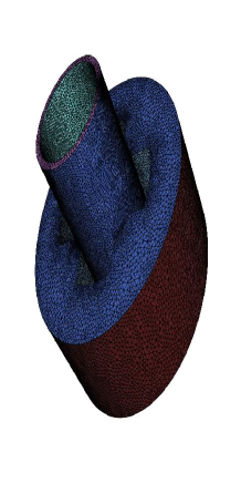
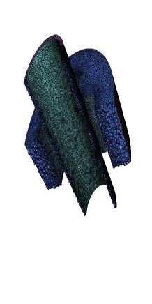
Figure 1: Triangulation of the conductive materials in the steam generator. Tube and Tube-support-plate (left), and their respective vertical-slice (right).

Taking into account the effect of the TSP using the 3D model, described above, which requires a very thin mesh size (proportional to the skin depth) inside the TSP and leads to a huge size of the discrete 3D problem. We hereafter explain how one can avoid integration over the volume of the TSP by imposing an appropriate impedance boundary condition (IBC) on its boundary $\Gamma_{p}$. More precisely it is shown in Duruflé et al. (2006) that electromagnetic field satisfies

$$\bm{\vec{n}}\times\frac{1}{\mu}\textbf{curl\hskip 0.72229pt}\mathbf{A}=-\dfrac{1}{\mathcal{Z}_{\Gamma_{p}}}(i\omega\mathbf{A}_{\tau}+{\bf\nabla V}_{c,\tau}),\quad\text{ on }\Gamma_{p}.$$ (12)

(up to $O(\delta^{2})$) on $\Gamma_{p}$. In the above equation; $\mathcal{Z}_{\Gamma_{p}}:=(1-i)/(\delta\sigma)$ with the skin depth $\delta:=\sqrt{2/(\omega\mu\sigma)}$ and the tangential component of the vector field $\mathbf{A}_{T}=\bm{\vec{n}}\times\big{(}\mathbf{A}\times\bm{\vec{n}}\big{)}$ (same apply for $\textbf{V}_{c}$). Therefore, if $\delta$ is sufficiently small i.e. $\omega\sigma_{p}\mu$ is sufficiently large and Eq. (12) is a very good approximation.

The impedance surface term of the weak formulation of Eq. (4) at the interface $\Gamma_{p}$ of the TSP is written:

$$\footnotesize\int_{\Gamma_{p}}\!\!\!\!\!\!\!\big{(}\bm{\vec{n}}\times(\frac{1}{\mu_{p}}\textbf{curl\hskip 0.72229pt}\mathbf{A})\big{)}\cdot\overline{\Phi_{\tau}}\,\delta s=\dfrac{-1}{\mathcal{Z}_{\Gamma_{p}}}\!\!\!\int_{\Gamma_{p}}\!\!\!\!(i\omega\mathbf{A}_{\tau}+\nabla_{\tau}\textbf{V}_{c})\cdot\overline{\Phi_{\tau}}\,\delta s$$ (13)

$$\footnotesize\int_{\Gamma_{p}}\!\!\!\!\!\!\!\sigma_{p}(i\omega\mathbf{A}+\nabla\textbf{V}_{c})\cdot\bm{\vec{n}}\,\overline{\varphi}\,\delta s=\\ \dfrac{-1}{\mathcal{Z}_{\Gamma_{p}}}\int_{\Gamma_{p}}\!\!\!\!(i\omega\mathbf{A}_{\tau}+\nabla_{\tau}\textbf{V}_{c})\cdot\overline{\nabla_{\tau}\varphi}\,\delta s,$$ (14)

We refers for instance to Haddar and Riahi (2013) for details related to the update on the variational formulation with respect to the impedance boundary condition. Here, we shall consider the general case in the numerical experiments, which consist of the volume representation of the TSP in the variational formulation.

The mathematical formulation for the evaluation of the electric impedance $\mathbf{Z}$ see Auld and Moulder (1999). It is common to use the following types of signals

$$\begin{cases}{\bf Z}_{FA}=\frac{i}{2}\big{(}\Delta\mathbf{Z}_{11}+\Delta\mathbf{Z}_{12}\big{)},\\ {\bf Z}_{F3}=\frac{i}{2}(\Delta\mathbf{Z}_{11}-\Delta\mathbf{Z}_{22}\big{)}.\end{cases}$$ (15)

which are respectively the absolute signal mode and the differential signal mode. The term $\mathbf{Z}_{kl}$ with $k,l$ in $\{1,2\}$ represents the volume impedance measured with the coil $k$ in the electromagnetic field induced by the coil $l$. It is written:

$$\displaystyle\Delta\mathbf{Z}_{kl}:=\frac{1}{i\omega}\frac{\mu_{\epsilon}-\mu_{d}}{\mu_{d}\mu_{\epsilon}}\int_{\Omega_{d}}\big{(}\textbf{curl\hskip 0.72229pt}\mathbf{A}_{k}\cdot\textbf{curl\hskip 0.72229pt}\mathbf{A}_{l}^{\epsilon}\big{)}\,\delta v$$

$$+(\sigma-\sigma_{\epsilon})\!\!\!\int_{\Omega_{d}}\!\!\!\!\!(i\omega\mathbf{A}_{k}+\nabla\textbf{V}_{c})\cdot(i\omega\mathbf{A}_{\tau,l}^{\epsilon}+{\bf\nabla V}^{\epsilon}_{c,l,\tau})\,\delta v,$$ (16)

where $i\omega\mathbf{A}_{\tau,l}^{\epsilon}+{\bf\nabla V}^{\epsilon}_{c,l,\tau}:=:\mathbf{E}_{l,\tau}^{0}$ refers to the tangential component of the electric field propagating in "vacuum". Rigorously one has to take care of the presence of loop field Alonso Rodríguez et al. (2013) in the vacuum. Their presence is related to the geometry of the computational domain (see Alonso Rodríguez and Valli (2010); Bossavit (2004) and reference therein).

Remark 2.1.

As eddy-current approximation of the Maxwell equation can be seen as the limit when the permittivity $\varepsilon$ tends to zero in Maxwell equations. We may use the vacuum as a medium with very low permittivity. In our case we consider a very low conductivity $\sigma_{\epsilon}\approx\epsilon<<1$ to describe the vacuum instead.

3 Numerical method

We describe in this section our numerical method which consists of the resolution of the coupled systems that solve the eddy-current problems necessary for the evaluation of the electric impedance $\mathbf{Z}$ defined at Eq. (15). We describe the major steps for the non-destructive test procedure and give details related to the resolution where numerical decisions have been made in order to better handle big ill-conditioned systems.

We suppose from now on, that the computational domain $\Omega$ is a Lipschitz polyhedra in $\mathbb{R}^{3}$, practically $\Omega$ represent the cylinder that envelops the Tube and the TSP. Once the computational domain is fixed, we then introduce a family of triangulation $\mathcal{T}_{\natural}$ of $\Omega$, the subscript $\natural$ stands for the largest length of the edges of the triangles that constitute $\mathcal{T}_{\natural}$. The Tetrahedrons of $\mathcal{T}_{\natural}$ match on the interface between the conductive part, i.e. tube and TSP ($\sigma\neq 0$) and the insulator part ($\sigma=0$). The triangulations of the conductive part are is in Figure 1.

The electric field $\mathbf{E}\equiv(\mathbf{A},\textbf{V}_{c})$ solution of the eddy current equation belongs to $H(\textbf{curl\hskip 0.72229pt},\Omega)\cap H(\textbf{div},\Omega)\times H^{1}(\Omega_{c})$. The fact that our computational domain (Cylinder as mentioned before) is a convex polyhedron is very important. It turns out that the space of smooth tangential vector fields $H_{\tau}^{1}(\Omega):=\big{(}H^{1}(\Omega)\big{)}^{3}\cap H(\textbf{div},\Omega)$ coincides with the proper close subspace of $H(\textbf{curl\hskip 0.72229pt},\Omega)\cap H(\textbf{div},\Omega)$. Thanks to this nice property, a finite element numerical approximation based on a nodal finite element will be considered for the electric vector potential $\textbf{V}_{c}$ as well as for the magnetic vector potential $\mathbf{A}$ Biro and Valli (2007). The infinite dimensional space $H_{\tau}^{1}(\Omega)\times H^{1}(\Omega)$ is therefore approximated with the finite-dimensional space $\mathcal{W}_{\natural}:=\mathcal{V}_{\natural}\times\mathcal{C}_{\natural}$, where $\mathcal{V}_{\natural}$ and $\mathcal{C}_{\natural}$ represent the discrete spaces of Lagrange nodal elements defined respectively as

$$\mathcal{V}_{\natural}:=\{{\bf v}_{\natural}\in(C^{0}(\Omega))^{3}|{\bf v}_{\natural_{|K}}\in(\mathbb{P}_{1})^{3},\forall K\in\mathcal{T}_{\natural},$$

$${\bf v}_{\natural}.\bm{\vec{n}}=0\text{ on }\partial\Omega\}$$

and $\mathcal{C}_{\natural}:=\{c_{\natural}\in C^{0}(\Omega_{c})|v_{\natural_{|K}}\in\mathbb{P}_{1},\forall K\in\mathcal{T}_{c,\natural}\}$.

In the above $\mathbb{P}_{1}$ stands for the space of polynomials of degree less than or equal to $1$. In addition, the boundary conditions ($\mathbf{A}\cdot\bm{\vec{n}}=0$ on $\partial\Omega$) are taken into account via penalization of the vortices that belong on the boundaries.Again thanks to geometric property of our computational domain, imposing this kind of boundary condition becomes trivial.

As stated earlier, the scan procedure consists in moving the probe according to the z-direction all the way through the tube. This leads to a set of scan positions where at each position we need to solve an ill-conditioned huge system. In addition to that, for any position one has to rebuild the triangulation and reassemble the matrices. To avoid this handicap we are led to consider a unique triangulation that includes all probe positions and then consider a factorization using a sophisticated software.

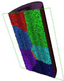
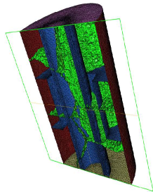
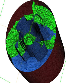
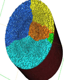
Figure 2: Partition of the Triangulation of the computational domain. Volume tetrahedrons surfaces are presented in top left and bottom right, the other plot correspond to the interfaces as required by the geometry of the SG and also interfaces generated by the partition.

In order to proceed with the parallelization, let us consider $P$ partitions of the computational domain $\Omega$, such that $\Omega=\cup_{p=1}^{P}\Omega^{p}$. We notice here that the partition is made in terms of the triangulation see Figure 2, where after the construction of the mesh, we partition its triangulations using a graph partitioner (e.g. Scotch Pellegrini (2001) or Metis Karypis and Kumar (1995)).

Remark 3.1.

Both graph partitioners Scotch and Metis are interfaced with the software Freefem++ Hecht (2012), and their utilization is quite easy.

We give a sample Freefem++ script in Table 1, where the graph partition scotch is called at line 6 to build a piecewise function "balance" which takes different values on each subdomain. Freefem++ is therefore able to construct local triangulation according to the values of the function "balance" (see lines 11-12 of Table 1). We notice that the construction of the function "balance" is performed only on the master processor with rank zero. The function "balance" is thus broadcasted to all processors through MPI (see line 9 of Table 1). We use this technique to ensure that all processors receive the same function balance and construct a uniform triangulation.

The numerical simulation of the ECT procedure reads as follows

1. Read/build a triangulation of the computational domain $\Omega$

2. Partition the triangulation with respect to the arbitrary choice (see command line in Tabular 1)

3. Assemble Morse type sparse-sub-matrices in parallel

4. All_reduce sparse-sub-matrices (This operation is achieved with MPI_SUM operation)

5. LU factorization of the global matrix.

6. Solve the set of problems $P_{i}$ by uniquely changing the right-hand side source term (accordingly to the position of the probe position)

7. Print out the impedance value results in an append writing file (to be sorted).

Let $\Phi_{\natural}\in\mathcal{V}_{\natural}$ and $\varphi_{\natural}\in\mathcal{C}_{\natural}$ be test functions for our coupled eddy-current problem, we denote by $\mathbf{A}_{\natural}$ and $\textbf{V}_{c,\natural}$ our unknowns. Local matrices need the following variational formulation in order to be assembled

$$\mathcal{L}^{p}_{11}\big{(}\mathbf{A}_{\natural},\Phi_{\natural}\big{)}\!\!\!\!\!\! = \!\!\!\!\!\!\sum_{K\in\mathcal{T}_{h}\subset\Omega^{p}}\int_{K}\dfrac{1}{\mu}\textbf{curl\hskip 0.72229pt}\mathbf{A}_{\natural}\cdot\overline{\textbf{curl\hskip 0.72229pt}\Phi_{\natural}}\,\delta v,$$ (17)

$$+\dfrac{1}{\tilde{\mu}}\int_{K}\textbf{div}\mathbf{A}_{\natural}\overline{\textbf{div}\Phi_{\natural}}\,\delta v$$

$$\mathcal{L}^{p}_{12}\big{(}\textbf{V}_{c,\natural},\Phi_{\natural}\big{)}\!\!\!\!\!\! = \!\!\!\!\!\!-\!\!\!\!\sum_{K\in\mathcal{T}_{h}\subset\Omega_{c}^{p}}\int_{K}\sigma\textbf{V}_{c,\natural}\cdot\overline{\Phi_{\natural}}\,\delta v.$$ (18)

$$\mathcal{L}^{p}_{21}\big{(}\mathbf{A}_{\natural},\varphi_{\natural}\big{)}\!\!\!\! = \!\!\!\!-\!\!\!\!\sum_{K\in\mathcal{T}_{h}\subset\Omega_{c}^{p}}\int_{K}\sigma\mathbf{A}_{\natural}\cdot\overline{\nabla\varphi_{\natural}}\,\delta v,$$ (19)

$$\mathcal{L}^{p}_{22}\big{(}\textbf{V}_{c,\natural},\varphi_{\natural}\big{)}\!\!\!\!\!\! = \!\!\!\!\!\!-\dfrac{1}{i\omega}\!\!\!\!\!\!\sum_{K\in\mathcal{T}_{h}\subset\Omega_{c}^{p}}\int_{K}\sigma\textbf{V}_{c,\natural}\cdot\overline{\nabla\varphi_{\natural}}\,\delta v.$$ (20)

We give in Table 2 a sample-freefem script that shows how to implement such bilinear forms.

$$\begin{array}[]{lr}{\bf M}_{11}=\sum_{p=1}^{P}M^{p}_{11},&\text{ with }{M}^{p}_{11}=\mathcal{L}^{p}_{11}(\Phi_{\natural},\Phi_{\natural}),\\ {\bf M}_{12}=\sum_{p=1}^{P}M^{p}_{12},&\text{ with }{M}^{p}_{12}=\mathcal{L}^{p}_{12}(\varphi_{\natural},\Phi_{\natural}),\\ {\bf M}_{21}=\sum_{p=1}^{P}M^{p}_{21},&\text{ with }{M}^{p}_{21}=\mathcal{L}^{p}_{21}(\Phi_{\natural},\varphi_{\natural}),\\ {\bf M}_{22}=\sum_{p=1}^{P}M^{p}_{22},&\text{ with }{M}^{p}_{22}=\mathcal{L}^{p}_{22}(\varphi_{\natural},\varphi_{\natural}).\end{array}$$

Remark 3.2.

The sparse matrice summations above are performed through the MPI Reduce operation. Thanks to the Morse sparse format of the matrices, the summations is not a term-by-term addition, but it increases the dimension at each sum, because of the assembly in disjoint subdomains; also all assembly uses the same mesh numbering.

The full discretized system thus reads

$$\left(\begin{array}[]{cc}{\bf M}_{11}&{\bf M}_{12}\\ {\bf M}{}_{21}&{\bf M}_{22}\end{array}\right)\left(\begin{array}[]{l}\mathbf{A}_{\natural}\\ \textbf{V}_{c,\natural}\end{array}\right)=\left(\begin{array}[]{l}{\mathbf{J}_{e}}_{,\natural}\\ {\bf 0}\end{array}\right)$$

The right hand side vector ${\mathbf{J}_{e}}_{,\natural}$ stands for the source term, which is basically given by the multiplication of the mass matrix by the interpolation of the analytic source term $\mathbf{J}_{e}$.

⬇

1 int[int] nupart(Th.nt);

2 fespace p0h(Th,P03d);

3 p0h balance;

4 int npart=mpisize;

5 if(mpirank==0){

6 scotch(nupart, Th, npart);

7 for(int i=0;i<Th.nt;i++)

8 balance[][i] = nupart[i];}

9 broadcast(processor(0,com),balance[]);

10 Th3[int] Thpart(npart);

11 for(int i=0;i<npart;i++) {

12 Thpart[i]=trunc(Th,balance==i);

13 Thpart[i]=change(Thpart[i],fregion=i);}

14 Th=Thpart[0];

15 for(int i=1;i<npart;i++) Th=Th+Thpart[i];

Table 1: Mesh partitioning – Freefem++ script sample.

⬇

1varf L11([Ax,Ay,Az],[Bx,By,Bz]) =

2 int3d(Th,mpirank)(1/mu*curl(Bx,By,Bz)*curl(Ax,Ay,Az) )

3 - int3d(Th,mpirank)( iomega*mu*sigma* [Bx,By,Bz]*[Ax,Ay,Az] )

4 + int3d(Th,mpirank)((div(Bx,By,Bz))*(div(Ax,Ay,Az)))

5 + on(labelup,labeldown,Az=0.)

6 + on(labelmid,Ax=0., Ay=0.);

7varf L22(V,qhc) =

8 int3d(ThC,mpirank)( (-1/iomega) * (

9 mu*sigmaEpsilon* [dx(qhc),dy(qhc),dz(qhc)]*[dx(V),dy(V),dz(V)] )

10 + delta*mu*sigma*V*qhc ) );

11varf L12([V],[Bx,By,Bz]) =

12 - int3d(ThC,mpirank)( mu*sigma* ( dx(V)*Bx+dy(V)*By+dz(V)*Bz) );

13varf L21([Ax,Ay,Az],[qhc]) =

14 - int3d(ThC,mpirank)( mu*sigma* [dx(qhc),dy(qhc),dz(qhc)]*[Ax,Ay,Az] );

Table 2: Variational formulation definition for the coupled problem – Freefem++ script sample.

⬇

1matrix <complex> M11,Mp11= L11(VPh,VPh);

2matrix <complex> M22,Mp22= L22(PhC,PhC);

3matrix <complex> M12,Mp12= L12(PhCS,VPh);

4matrix <complex> M21,Mp21= L21(VPh,PhCS);

Table 3: Matrix Assembly, with Morse sparse forma – Freefem++ script sample.

⬇

1mpiAllReduce(Mp11,M11,mpiCommWorld,mpiSUM);

2mpiAllReduce(Mp12,M12,mpiCommWorld,mpiSUM);

3mpiAllReduce(Mp21,M21,mpiCommWorld,mpiSUM);

4mpiAllReduce(Mp22,M22,mpiCommWorld,mpiSUM);

5matrix<complex> M = [[M11,M12],

6 [M21,M22]];

7set(M,solver=sparsesolver,eps=1.e-16);

Table 4: Reduce Morse sparse matrix – Freefem++ script sample.

The boundary condition $\mathbf{A}\cdot\bm{\vec{n}}=0$ on the exterior boundary $\partial\Omega$ are taken into account using the penalization term, where the linear system is forced to take into account the given values at the boundary mesh points.

4 Numerical Experiments

In our application we consider that the excitation source term $\mathbf{J}_{e}$ is uniformly distributed on a support included in $\Omega_{I}$ (principally it models the solenoid source coil of the probing problem). So, let $\mathbf{J}_{e}\in(L^{2}(\Omega))^{3}$ with $\textbf{div}\mathbf{J}_{e}=0$ in $\Omega_{I}$ as $\mathbf{J}_{e}:=:{[-y_{|_{\Omega_{I}}},x_{|_{\Omega_{I}}},0]}/{\sqrt{x^{2}+y^{2}}}$.

As the electric scalar potential $\textbf{V}_{c}$ is determined up to an additive constant, we may numerically impose a supplement condition such that $\int_{\Omega_{c_{i}}}\!\!\!\!\!\!\nabla\textbf{V}_{c}\,\delta v=0$ ($\Omega_{c_{i}}$ is any connex component subset of $\Omega_{c}.$). This also could be incorporated under the global problem by penalization $\delta\sigma\nabla\textbf{V}_{c},\text{ in }\Omega_{c},\text{ with a small }\delta<<1.$ Therefore we augment the variational formulation $\mathcal{L}^{p}_{22}$ by the former penalization integration.

P in MPI	$\text{Assemble}\left(M^{0}_{i}\right)$	$\text{Reduce}\left(M^{0}\right)$	$LU|^{0}$
1	3144.68	–	585.28
2	1202.98	585.74	440.36
4	758.73	575.86	582.76
8	312.08	512.76	501.25
16	163.87	591.56	596.33
32	88.74	542.30	577.28
64	19.02	516.50	562.61

Table 5: Parallel Performance in wall-clock time in seconds for the problem without TSP as default. This means the numerical simulation takes the region of the TSP as a "vacuum".

P in MPI	$\text{Assemble}\left(M^{1}_{i}\right)$	$\text{Reduce}\left(M^{1}\right)$	$LU|^{1}$
1	3237.47	-	341.22
2	1284.52	392.18	332.61
4	764.47	587.49	332.44
8	311.28	687.63	497.75
16	177.14	647.32	368.43
32	42.37	583.32	328.61
64	19.55	598.87	350.10

Table 6: Parallel Performance in wall-clock time in seconds for the problem with TSP.

We give in Table 5 and Table 6 the performance in term of the execution (wall-clock) time in seconds of our numerical method. In Table 5 (respectively Table 6) we report results related to the system without TSP as default (respectively with TSP region as default), where the computed matrix has size $n\times m=991.246\times 991.246$ (respectively $n\times m=1.069.595\times 1.069.595$) with $46.664.492$ (respectively $54.350.718$) non-zero coefficients. It is worth recalling that these calculations are necessary for the evaluation of the impedance signals Eq. (2). As the results indicate, the most memory and time consuming task (the main matrix for the coupled system) is mitigated through high performance computing using parallel resources, where scalability of the operation is clearly exhibited. MPI communications are thus necessary to collect local Morse sparse matrices. These operations, thanks to the optimized communication technique, enable the maintenance of a reasonable average of performance despite the increase of the communicators number. Actually, this fact is balanced with the size of the message that has to be transferred. Indeed, as the communicators numbers increases, the size of the morse sparse matrices decreases. Once the global matrix is assembled and copied (via MPI) to all processors, we are then able to perform a fast factorization. In Figure 3 we plot the intensity of the computed electric field when the probe is near to the TSP. We have used Super_LU Li (2005) parallel direct solver for the factorization. This procedure has also a good performance while using several processors. As the scan procedure is parallel by nature (each probe position is totally independent of other positions). Therefore, parallel resources share the effort of solving independently coupled systems according to different probe positions. We report in Figure 4 the robustness of our method in term of speedup while increasing the number of parallel processors $P$. We evaluate the speedup formula given by $S^{p}=\text{t}_{\text{tot}}^{p}/t^{\text{serial}}$ with $\text{t}_{\text{tot}}^{p}=\text{t}_{\text{Assemble}}^{p}+\text{t}_{\text{Reduce}}^{p}+\text{t}_{\text{Factorize}}^{p}+\text{t}_{\text{Solve}}^{p}$. We have considered $128$ probe positions for the scan procedure where the time to solve the problem is in average $40$ minutes. The results exhibit the fact that our method is fully efficient and scalable in term of parallelism.

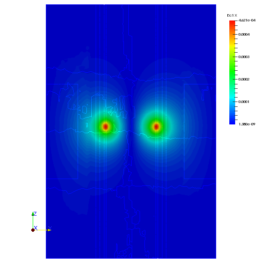
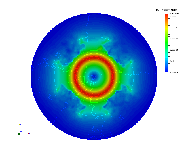
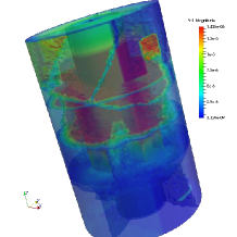
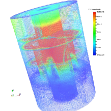
Figure 3: The intensity of the computed Electric field $\mathbf{E}=i\omega\mathbf{A}+\nabla\textbf{V}_{c}$: YZ-plan slice projection (top left) and XY-plan slice projections (top right). Volume rescale plot (bottom left) and Wireframe projection rescaled plot (bottom right).

Figure 4: Speedup of the numerical method.

5 Conclusions

We have presented in this paper a finite element technique that enables a rapid numerical simulation of the ECT problem in SG. Our approach has been validated through the use of high performance computing in parallel machines. We have shown that our approach is full efficient and leads to a robust and rapid ECT in real life industrial problem.

References

- Alonso Rodríguez and Valli [2010] Ana Alonso Rodríguez and Alberto Valli. Eddy current approximation of Maxwell equations, volume 4 of MS&A. Modeling, Simulation and Applications. Springer-Verlag Italia, Milan, 2010. ISBN 978-88-470-1505-0. doi: 10.1007/978-88-470-1506-7. URL http://dx.doi.org/10.1007/978-88-470-1506-7. Theory, algorithms and applications.
- Alonso Rodríguez et al. [2013] Ana Alonso Rodríguez, Enrico Bertolazzi, Riccardo Ghiloni, and Alberto Valli. Construction of a finite element basis of the first de Rham cohomology group and numerical solution of 3D magnetostatic problems. SIAM J. Numer. Anal., 51(4):2380–2402, 2013. ISSN 0036-1429. doi: 10.1137/120890648. URL http://dx.doi.org/10.1137/120890648.
- Ammari et al. [2000] H. Ammari, A. Buffa, and J.-C Nédélec. A justification of eddy currents model for the maxwell equations. SIAM J. Appl. Math., 60(5):1805–1823, May 2000. ISSN 0036-1399. doi: 10.1137/S0036139998348979. URL http://dx.doi.org/10.1137/S0036139998348979.
- Auld and Moulder [1999] B. A. Auld and J. C. Moulder. Review of advances in quantitative eddy current nondestructive evaluation. Journal of Nondestructive evaluation, 18(1):3–36, 1999.
- Bendjoudi et al. [2010] Aniss Bendjoudi, Emmanuel Bossy, Marie-Françoise Cugnet, Patrick Chauvin, and Didier Cassereau. Développement d’un logiciel hybride pour le Contrôle Non Destructif. In Société Française d’Acoustique SFA, editor, 10ème Congrès Français d’Acoustique, pages –, Lyon, France, 2010. URL http://hal.archives-ouvertes.fr/hal-00549199.
- Bíró and Valli [2007] Oszkár Bíró and Alberto Valli. The Coulomb gauged vector potential formulation for the eddy-current problem in general geometry: well-posedness and numerical approximation. Computer Methods in Applied Mechanics and Engineering, 196(13-16):1890–1904, 2007. ISSN 0045-7825. doi: 10.1016/j.cma.2006.10.008. URL http://dx.doi.org/10.1016/j.cma.2006.10.008.
- Biro and Valli [2007] Oszkar Biro and Alberto Valli. The coulomb gauged vector potential formulation for the eddy-current problem in general geometry: well-posedness and numerical approximation. Computer methods in applied mechanics and engineering, 196(13):1890–1904, 2007.
- Bossavit [2004] Alain Bossavit. Electromagnetisme, en vue de la modelisation, volume 14. Springer Science & Business Media, 2004.
- Duruflé et al. [2006] Marc Duruflé, Houssem Haddar, and Patrick Joly. Higher order generalized impedance boundary conditions in electromagnetic scattering problems. Comptes Rendus Physique, 7(5):533–542, 2006.
- Girard [2014] Sylvain Girard. Clogging of recirculating nuclear steam generators. In Physical and Statistical Models for Steam Generator Clogging Diagnosis, pages 3–13. Springer, 2014.
- Haddar and Jiang [2015] Houssem Haddar and Zixian Jiang. Axisymmetric eddy current inspection of highly conducting thin layers via asymptotic models. Inverse Problems, 31(11):115005, 2015.
- Haddar and Riahi [2013] Houssem Haddar and Mohamed Kamel Riahi. 3D direct and inverse solvers for eddy current testing of deposits in steam generator. Technical report, July 2013. URL https://hal.inria.fr/hal-01044648.
- Hecht [2012] F. Hecht. New development in freefem++. Journal of Numerical Mathematics, 20(3-4):251–265, 2012. ISSN 1570-2820.
- Huang and Takagi [2000] Haoyu Huang and Toshiyuki Takagi. Crack shape reconstruction from noisy signals in ect of steam generator tube. In Industrial Electronics Society, 2000. IECON 2000. 26th Annual Conference of the IEEE, volume 4, pages 2507–2512. IEEE, 2000.
- Huang et al. [2000] Haoyu Huang, T. Takagi, and H. Fukutomi. Fast signal predictions of noised signals in eddy current testing. Magnetics, IEEE Transactions on, 36(4):1719–1723, Jul 2000. ISSN 0018-9464. doi: 10.1109/20.877774.
- Karypis and Kumar [1995] George Karypis and Vipin Kumar. Metis - unstructured graph partitioning and sparse matrix ordering system, version 2.0, 1995.
- Li [2005] Xiaoye S. Li. An overview of SuperLU: Algorithms, implementation, and user interface. ACM Transactions on Mathematical Software, 31(3):302–325, September 2005.
- Pellegrini [2001] François Pellegrini. Scotch and libscotch 3.4 user’s guide, 2001.
- Takagi et al. [1997] Toshiyuki Takagi, Junji Tani, Hiroyuki Fukutomi, and Mitsuo Hashimoto. Finite element modeling of eddy current testing of steam generator tube with crack and deposit. In DonaldO. Thompson and DaleE. Chimenti, editors, Review of Progress in Quantitative Nondestructive Evaluation, volume 16 of Review of Progress in Quantitative Nondestructive Evaluation, pages 263–270. Springer US, 1997. ISBN 978-1-4613-7725-2. doi: 10.1007/978-1-4615-5947-4_34. URL http://dx.doi.org/10.1007/978-1-4615-5947-4_34.
- The Open Access NDT Database [2014] The Open Access NDT Database. The web’s largest database of nondestructive testing (NDT) conference proceedings, articles, news, exhibition, forum and a professional network. NDT Database and Journal of Nondestructive Testing - NDT, Ultrasonic Testing, X-Ray, Radiography, Eddy Current and All NDT Methods., 2014. URL http://www.ndt.net/index.php.
- Tian et al. [2005] Gui Yun Tian, A. Sophian, D. Taylor, and J. Rudlin. Multiple sensors on pulsed eddy-current detection for 3-d subsurface crack assessment. Sensors Journal, IEEE, 5(1):90–96, Feb 2005. ISSN 1530-437X. doi: 10.1109/JSEN.2004.839129.