Isotropic at the Break? 3D Kinematics of Milky Way Halo Stars in the Foreground of M31

Abstract

We present the line-of-sight (LOS) velocities for 13 distant main sequence Milky Way halo stars with published proper motions. The proper motions were measured using long baseline (5–7 years) multi-epoch HST/ACS photometry, and the LOS velocities were extracted from deep (5–6 hour integrations) Keck II/DEIMOS spectra. We estimate the parameters of the velocity ellipsoid of the stellar halo using a Markov chain Monte Carlo ensembler sampler method. The velocity second moments in the directions of the Galactic $(l,b,$ LOS) coordinate system are $\langle v^{2}_{l}\rangle^{1/2}=138^{+43}_{-26}$ km s^-1, $\langle v^{2}_{b}\rangle^{1/2}=88^{+28}_{-17}\ \mbox{km \ s}^{-1}$, and $\langle v^{2}_{\rm{LOS}}\rangle^{1/2}=91^{+27}_{-14}\ \mbox{km \ s}^{-1}$. We use these ellipsoid parameters to constrain the velocity anisotropy of the stellar halo. Ours is the first measurement of the anisotropy parameter $\beta$ using 3D kinematics outside of the solar neighborhood. We find $\beta=-0.3^{+0.4}_{-0.9}$, consistent with isotropy and lower than solar neighborhood $\beta$ measurements by 2$\sigma$ ($\beta_{SN}\sim 0.5-0.7$). We identify two stars in our sample that are likely members of the known TriAnd substructure, and excluding these objects from our sample increases our estimate of the anisotropy to $\beta=0.1^{+0.4}_{-1.0}$, which is still lower than solar neighborhood measurements by $1\sigma$. The potential decrease in $\beta$ with Galactocentric radius is inconsistent with theoretical predictions, though consistent with recent observational studies, and may indicate the presence of large, shell-type structure (or structures) at $r\sim 25$ kpc. The methods described in this paper will be applied to a much larger sample of stars with 3D kinematics observed through the ongoing HALO7D program.

1. Introduction

The Milky Way halo devours hundreds of lower mass dwarf galaxies over its lifetime. The stripped stellar material from this voracious eating habit is splayed out in a vast, diffuse stellar halo. The orbital timescales at these large distances ($\gtrsim$ 10 kpc) are very long, and the halo stars retain a memory of their initial conditions. Thus, by studying the phase space distribution of halo stars, we are privy to a unique window into the past accretion history of our Galaxy.

Global kinematic properties, such as the velocity anisotropy (i.e., the relative pressure between tangential and radial velocity components), can provide important insight into the formation of the stellar halo (see Binney & Tremaine 2008). The exact merger and dissipation history of a spheroid can strongly affect its velocity anisotropy profile (e.g., Naab et al. 2006; Deason et al. 2013a). Local studies, limited to heliocentric distances $D\lesssim 10$ kpc, have measured the full 3D kinematics of halo stars. This has revealed a strongly radially biased velocity anisotropy with $\beta=1-\sigma^{2}_{\rm tan}/\sigma^{2}_{\rm rad}\approx 0.5-0.7$ (e.g., Smith et al. 2009; Bond et al. 2010), in seemingly good agreement with the predictions of simulations (e.g., Bullock & Johnston 2005; Cooper et al. 2010).

In Deason et al. (2013b) (hereafter D13), we exploited the long time-baselines and exquisite photometry of deep, multi-epoch HST fields to measure the proper motions (PMs) of main sequence turn-off (MSTO) stars in the distant Milky Way halo. Our pilot program used 5–7 year baseline HST/ACS fields towards M31 to measure PMs of $N\sim 13$ halo stars in the foreground. Our PMs are extremely accurate, with random errors of $\sim$ 5 km s^-1. These 13 halo stars provided the first direct bound on the tangential velocity moments of the halo in this extreme radial regime, and provide new insights into halo structure. From the PMs measured for 13 Milky Way halo stars at 18 $\lesssim$ $r$ $\lesssim$ 30 kpc in our M31 HST fields, D13 inferred approximate isotropy between radial and tangential motions: $\beta$ = 0.0${}^{+0.2}_{-0.4}$. This differs by $3\sigma$ from local measures of the velocity anisotropy, which find strongly radial orbits. This trend of decreasing radial anisotropy with galactocentric distance conflicts with numerical simulations, which predict an outward increase in radial anisotropy.

In D13, we had no line-of-sight (LOS) information for these stars: we relied on the LOS velocities of other halo tracers (blue horizontal branch (BHB) stars, K giants) in different regions of the sky to form our argument. With spectroscopic information, we circumvent the need to rely on independent, and perhaps biased, tracers. In this paper, we present the LOS velocities for our halo star candidates, and use this 3D kinematic information to estimate the parameters of the velocity ellipsoid and the velocity anisotropy.

The paper is arranged as follows. In Section 2, we describe the target selection, proper motion measurements, spectroscopic observations and LOS velocity extraction. In Section 3, we describe our method for estimating the parameters of the velocity ellipsoid. Our results are presented in Section 4, and discussed in Section 5. We summarize our findings in Section 6.

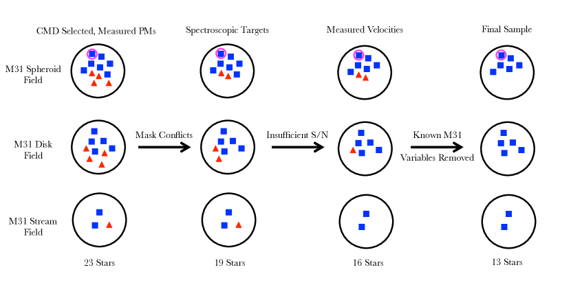
Figure 1.— Visual representation of the evolution of our sample, from the 23 CMD-selected halo star candidates from D13 to our sample of 13 stars. The different symbols represent the classification of the stars based on their proper motions: red triangles are M31 star candidates, while blue squares are Milky Way stars (see Fig. 3 of D13). The pink circle denotes the object classified as a potential Milky Way disk star in D13.

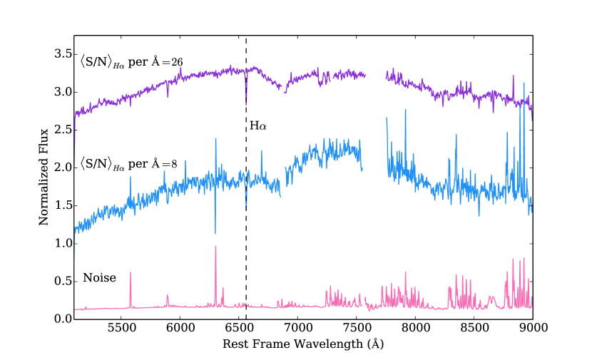
Figure 2.— Two sample stellar spectra from our sample: one of our higher signal-to-noise spectra (S/N per Å=26) is shown in purple and a lower signal-to-noise spectrum (S/N per Å=8) is shown in blue. The noise spectrum for the lower signal-to-noise spectrum is shown on the bottom in pink. The spectra have been normalized, smoothed with a Gaussian kernel with $\sigma=3$, and plotted with a vertical offset. We mask the chip gap in each spectrum, as well as the telluric A band at 7600 $\rm{\AA}$ and the telluric B band at 6875 Å. The dip in the spectra between 6700 $\rm{\AA}$ and 7200 $\rm{\AA}$ is an instrumental feature. Spikes in the noise spectrum correspond to night sky emission lines. The signal to noise ratios are computed at H$\alpha$.

Field	RA (J2000)	DEC (J2000)	$m_{\mathrm{F814W}}$	$m_{\mathrm{F606W}}$	$\mu_{l}$ [mas yr-1]	$\mu_{b}$ [mas yr-1]	$v_{\rm{LOS}}$ (GSR) [km s-1]	S/N per Å
M31 Spheroid
	00:46:01.47	+40:41:35.53	21.86	21.45	$-1.96\pm 0.04$	$-2.08\pm 0.04$	$54\pm 8^{*}$	19.4
	00:46:03.79	+40:41:22.81	22.53	22.19	$1.36\pm 0.02$	$-1.33\pm 0.02$	$-68\pm 17$	9.3
	00:46:03.67	+40:41:56.60	22.88	22.52	$2.12\pm 0.03$	$-0.82\pm 0.02$	$-90\pm 19$	9.4
	00:46:06.41	+40:42:15.07	22.53	22.06	$1.45\pm 0.02$	$-0.90\pm 0.02$	$37\pm 16$	10.5
	00:46:05.14	+40:43:37.19	21.82	21.47	$3.91\pm 0.02$	$-1.59\pm 0.02$	$120\pm 6$	20.9
	00:46:12.92	+40:41:22.51	22.92	22.61	$1.88\pm 0.06$	$-2.83\pm 0.06$	$43\pm 15^{*}$	8.1
M31 Disk
	00:49:08.91	+42:44:13.62	21.79	21.40	$-0.59\pm 0.03$	$-1.50\pm 0.04$	$73\pm 4$	30.0
	00:49:08.30	+42:44:50.44	22.12	21.66	$+1.03\pm 0.04$	$-0.78\pm 0.04$	$-42\pm 6$	26.0
	00:49:13.50	+42:43:36.17	22.71	22.35	$-0.71\pm 0.07$	$-0.67\pm 0.08$	$-117\pm 10$	15.9
	00:49:13.38	+42:45:56.93	23.62	23.30	$+2.16\pm 0.05$	$-0.40\pm 0.06$	$142\pm 39$	7.2
	00:49:13.69	+42:45:52.07	24.76	24.29	$+0.64\pm 0.07$	$+0.58\pm 0.06$	$-175\pm 10$	12.2
M31 Stream
	00:44:26.44	+39:47:33.43	22.69	22.35	$+0.00\pm 0.06$	$-1.85\pm 0.06$	$-89\pm 7$	18.3
	00:44:23.93	+39:46:26.25	23.83	23.46	$-0.43\pm 0.05$	$-1.13\pm 0.07$	$16\pm 16$	6.9

Table 1The properties of the candidate halo stars with measured 3D kinematics used in this analysis. We give the right ascension (RA) and declination (DEC), HST/ACS STMAG magnitudes, PMs in Galactic coordinates and LOS velocity (in the Galactocentric frame). The RA, DEC and magnitudes come from Brown et al. (2009), and the proper motions derive from the study by Sohn et al. (2012). The LOS velocity measurements are described in Section 2.2.3. Potential TriAnd members are indicated by an asterisk. The signal to noise ratios are computed at H$\alpha$.

2. Dataset

2.1. HST Imaging: Proper Motions

A detailed description of the target selection can be found in D13, but we summarize the key points here. Our objects were selected from three HST observing programs: GO-9453, GO-10265 (PI: T.Brown), and GO-11684 (PI: R.P. van der Marel). The combination of these three programs provide deep, multi-epoch optical imaging of three fields in M31 (M31 Spheroid, M31 Disk and M31 Stream). These observations were used to measure the proper motion of M31 (Sohn et al. 2012), and during the course of this study, proper motion catalogs for individual stars in the three HST fields were created.

D13 selected Milky Way halo star candidates in color-magnitude space, using photometry from Brown et al. (2009): all stars fall within $m_{\mathrm{F606W}}-m_{\mathrm{F814W}}\sim-0.3$ and $21.5\lesssim m_{\mathrm{F814W}}\lesssim 25.5$. In this region of the color-magnitude diagram (CMD) we expect minimal contamination from the Milky Way disk and M31’s red giant branch (see Section 2.2 and Figure 1 of D13). Proper motions were then used to classify the objects as M31, Milky Way halo and Milky Way disk stars. The average uncertainty in the proper motion measurements is $\sigma_{\mu}\sim 0.05$ mas yr^-1.

2.2. Keck/DEIMOS Spectra

2.2.1 Spectroscopic Sample

Figure 1 demonstrates how our initial sample from D13 evolved into the sample used in this analysis. In D13, we presented proper motions for the 23 candidate halo stars selected from color-magnitude diagrams (CMDs): 11, 9, and 3 stars in the M31 Spheroid, M31 Disk and M31 Stream fields, respectively. Based on the proper motions, 13 of these stars were classified as Milky Way halo stars, 9 as M31 stars, and 1 as a potential Milky Way disk star (see Figure 3 of D13). The symbols in Figure 1 represent the proper motion classification: Milky Way halo star candidates are blue squares, M31 star candidates are red triangles, and the pink circle denotes the potential Milky Way disk star. We obtained spectra for 19 of the original 23 stars; we were not able to obtain spectra for all of the halo star candidates due to conflicts in the spectral direction on the DEIMOS slitmask. Three additional stars were too faint to measure velocities. After removing known variables in M31 (Brown et al. 2004; Jeffery et al. 2011), we were left with our final sample of 13 objects. It is worth noting that this is not the exact same sample of 13 stars used in the kinematic analysis of D13: one of the objects we used in D13 was very faint ($m_{\rm F814W}=24.05$) and without strong spectral features, so we were unable to measure its velocity. We include the object classified as a potential disk star in D13 in our analysis (as its LOS velocity is consistent with halo kinematics). The properties of our 13 stars are summarized in Table 1.

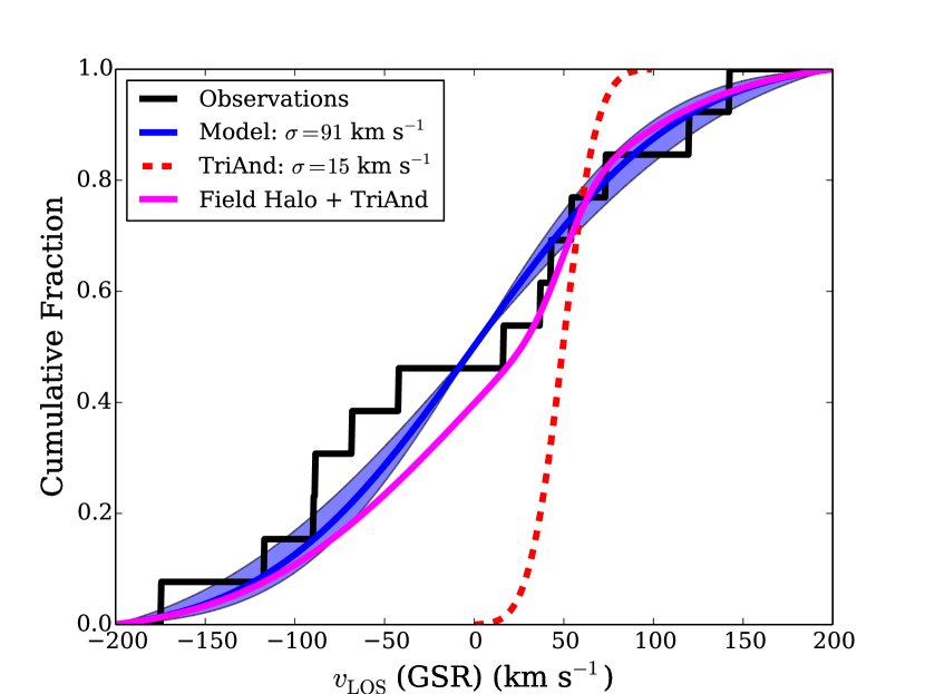
Figure 3.— Cumulative histogram of LOS velocities (in the Galactocentric frame) of the 13 halo stars in our sample (black). The overplotted blue line shows the CDF for the most likely value for $\sigma_{\rm{LOS}}$ for the full sample (see Sec. 3), with the shaded blue region indicating the 68% confidence region. An approximate CDF for the Triangulum-Andromeda Stream (TriAnd) is shown in red ($v_{0}\sim 50$ km s^-1, $\sigma\sim 15$ km s^-1). The pink line shows the CDF when the LOS velocity distribution is modelled as a double Gaussian, with TriAnd ($\sim 20\%$) and the field halo treated as separate components.

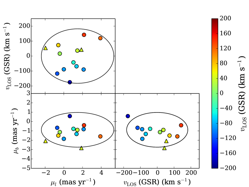
Figure 4.— Projections of our 3D kinematic sample, color coded by LOS velocity in the GSR frame. Likely TriAnd members are indicated by triangles. The ellipses show the 2D projection of the 3D velocity ellipsoid; the mean sample distance (20 kpc; see Table 2, Section 3) was used to convert from km s^-1 to mas yr^-1 for the proper motion axes. Ellipses are drawn to enclose 2$\sigma$.

2.2.2 Observations

Observations were taken on September 28–30, 2014 on the Keck II telescope with the DEIMOS spectrograph (Faber et al. 2003). Over the course of the run, the seeing varied from $0.45^{\prime\prime}-0.9^{\prime\prime}$. We observed one slitmask in each of the three fields with the 600 line/mm grating. The central wavelength was 7200 Å, resulting in a wavelength range of $\sim 4500-9300$ Å, where the exact wavelength range for each object varies depending on its position on the mask. The spectral resolution at $H\alpha$ (6563 Å) is $R\sim 2000$ (measured at the FWHM). In order to limit the flux losses due to atmospheric dispersion, we tilted our slits such that the position angle of the slit was consistent with the median parallactic angle of the observing block. The masks in the Spheroid and Disk fields were observed for a total of 5.9 hours, and the Stream field mask was observed for 5.3 hours. The slitmasks were then processed by a modified version of the spec2d pipeline developed by the DEEP2 team at UC Berkeley (Cooper et al. 2012). Two spectra from our sample are plotted in Figure 2; the top spectrum in Figure 2, shown in purple, has one of the higher signal-to-noise ratios of our sample (S/N per Å=26 at H$\alpha$), while the lower spectrum, shown in blue, is an example of one of our lower signal-to-noise objects (S/N per Å=8 at H$\alpha$). The noise spectrum from the lower signal-to-noise object is shown at the bottom of the figure in pink.

2.2.3 Velocity Measurements

Line-of-sight (LOS) velocities are measured from one-dimensional spectra using the Penalized Pixel-Fitting method (pPXF) of Cappellari & Emsellem (2004). The program determines the best fit composite stellar template for a given target using a penalized maximum likelihood approach. The 31 stellar templates employed in this analysis are described in detail in Toloba et al. (2016, submitted); the templates have high signal-to-noise ratios (100–800 $\rm{\AA}^{-1}$), and span a range of spectral types (from B1 to M8) and luminosity classes (from dwarfs to supergiants).

Errors in the raw velocity are determined through 1000 Monte Carlo simulations. In each simulation, we perturb the flux of the spectrum by adding noise to each pixel based on the uncertainty of the flux measurement in that pixel. The amount of noise added is drawn from a Gaussian distribution with width equal to the flux uncertainty. We then measure the velocity of each perturbed spectrum, and the error on the LOS velocity is taken to be the biweight standard deviation of the Gaussian distribution of velocities of perturbed spectra.

A-band telluric corrections are measured using the same method, and heliocentric LOS velocities are calculated by applying the A-band and heliocentric corrections to the raw velocities. The final uncertainty in the heliocentric LOS velocity is determined by adding in quadrature the errors on the raw velocity and the A-band correction.

Figure 4 shows a cumulative histogram of the LOS velocities for our sample of halo stars, in the frame of the Galactic Standard of Rest (GSR). Observed heliocentric velocities are converted to Galactocentric ones by assuming a circular speed of 240 km s^-1 (e.g., Reid et al. 2009; McMillan 2011; Schönrich 2012) at the position of the sun ($R_{0}=8.5$ kpc) with a solar peculiar motion ($U,V,W$)=(11.1, 12.24, 7.25) km s^-1 (Schönrich et al. 2010). Here, $U$ is directed toward the Galactic center, $V$ is positive in the direction of Galactic rotation and $W$ is positive towards the North Galactic Pole.

In Figure 4, we see evidence for a “hot halo” population: there are no sharp increases where we expect to see contamination from the Milky Way Disk (along this line of sight, $\langle v_{\rm{disk}}\rangle\sim 145$ km s^-1) or M31 ($\langle v_{\rm{M31}}\rangle\sim-150$ km s^-1). The blue curve shows the cumulative distribution function (CDF) for the $\sigma_{\rm{LOS}}$ value with maximum posterior probability (see Section 3), with the shaded blue region indicating the 68% confidence region. In contrast, as an example of substructure that is dynamically cold in LOS velocity, an approximate CDF for the Triangulum-Andromeda Stream (TriAnd; located along the line-of-sight towards M31) is shown in red ($v_{0}\sim 50$ km s^-1, $\sigma\sim 15$ km s^-1; e.g., Deason et al. 2014; Sheffield et al. 2014). D13 suggested that the presence of a cold stream or TriAnd could be the reason for the relative increase in tangential pressure seen in this sample. However, our LOS velocity measurements confirm that this is not the case: the significant dispersion in the LOS velocity distribution demonstrates that our sample is not dominated by members of a cold stream nor by TriAnd.

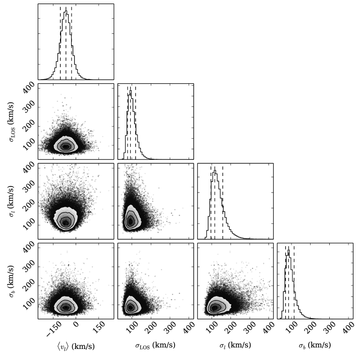
Figure 5.— Projections of the posterior probability distribution for our four free parameters, when the full sample of 13 objects was used. Contours are shown at 0.5, 1, 1.5 and 2 $\sigma$, respectively. The top panel in each column shows the 1D marginalized PDF for each parameter, with peaks and 68 % confidence intervals indicated by dashed vertical lines. We acknowledge the use of triangle.py (Foreman-Mackey et al. 2014) to produce this figure.

While the LOS velocity distribution confirms that our sample isn’t dominated by TriAnd, TriAnd members could still be biasing our measurement of the anisotropy. Given that our sample is in the same part of the sky and occupies the same region of CMD space as TriAnd (cf. Martin et al. 2014), we estimated the TriAnd contamination in our sample by fitting a double Gaussian to the LOS velocity distribution. The resulting fit revealed that we expect 2-3 TriAnd stars in our sample, though the underlying hot halo LOS dispersion only changes by $\sim 5\%$ (see Table 2). The two stars that most likely belong to TriAnd based on their LOS velocities also happen to lie directly over the TriAnd overdensity as seen in CMDs (see Figure 1 of Martin et al. (2014)). The third star with the LOS velocity closest to that of TriAnd lies off the CMD overdensity. We therefore conclude that two of our stars are likely members of TriAnd. The CDF for the double Gaussian best-fit is shown in pink in Figure 4.

Figure 4 summarizes our 3 dimensional kinematic sample, showing the Galactic proper motion components of the 13 halo stars color coded by LOS velocity. Our sample does not contain any members of M31, as all of these stars have proper motions too large to be associated with M31. As in Figure 4, Figure 4 shows no obvious clumpiness in any kinematic component, indicating that our sample is dominated by a “hot halo” population. However, it is intriguing that the two stars likely belonging to the TriAnd overdensity (shown as triangles in Figure 4) have relatively large proper motions. In the following sections, we consider the halo velocity ellipsoid both with and without the potential TriAnd stars.

Velocity Ellipsoid [km s-1]
Galactic coordinates
Full Sample	$\langle v^{2}_{\rm{LOS}}\rangle^{1/2}=91^{+27}_{-14}$	$\langle v^{2}_{b}\rangle^{1/2}=88^{+28}_{-17}$	$\langle v^{2}_{l}\rangle^{1/2}=138^{+43}_{-26}$	$\langle v_{l}\rangle=-67\pm 37$
Excluding TriAnd	$\langle v^{2}_{\rm{LOS}}\rangle^{1/2}=96^{+33}_{-15}$	$\langle v^{2}_{b}\rangle^{1/2}=82^{+35}_{-16}$	$\langle v^{2}_{l}\rangle^{1/2}=103^{+50}_{-17}$	$\langle v_{l}\rangle=-50^{+37}_{-40}$
Spherical polar coordinates
Full Sample	$\langle v^{2}_{r}\rangle^{1/2}=95^{+25}_{-14}$	$\langle v^{2}_{\theta}\rangle^{1/2}=85^{+29}_{-17}$	$\langle v^{2}_{\phi}\rangle^{1/2}=135^{+41}_{-20}$	$\langle v_{\phi}\rangle=65\pm 38$
Excluding TriAnd	$\langle v^{2}_{r}\rangle^{1/2}=100^{+30}_{-15}$	$\langle v^{2}_{\theta}\rangle^{1/2}=83^{+35}_{-15}$	$\langle v^{2}_{\phi}\rangle^{1/2}=118^{+50}_{-21}$	$\langle v_{\phi}\rangle=53\pm 39$
Velocity Anisotropy
Full Sample	$\beta=-0.3^{+0.4}_{-0.9}$	$\sqrt{\frac{\langle v^{2}_{t}\rangle}{\langle v^{2}_{r}\rangle}}=1.6^{+0.5}_{-0.4}$	$\sqrt{\frac{\langle v^{2}_{\phi}\rangle}{\langle v^{2}_{\theta}\rangle}}=1.4^{+0.6}_{-0.4}$
Excluding TriAnd	$\beta=0.1^{+0.4}_{-0.9}$	$\sqrt{\frac{\langle v^{2}_{t}\rangle}{\langle v^{2}_{r}\rangle}}=1.4^{+0.6}_{-0.3}$	$\sqrt{\frac{\langle v^{2}_{\phi}\rangle}{\langle v^{2}_{\theta}\rangle}}=1.3^{+0.6}_{-0.3}$
Position
	$l=121^{\circ}$	$b=-21^{\circ}$	$\langle D\rangle=20\pm 1\pm 7$ kpc	$\langle r\rangle=25\pm 1\pm 7$ kpc

Table 2Summary of our main results. We give the velocity ellipsoid in Galactic and spherical coordinate systems and the resulting velocity anisotropy, both for when we include all 13 stars and for when we exclude the 2 stars that are likely TriAnd members. We also give the approximate location of our three HST fields in the plane of the sky, as well as the average heliocentric and Galactocentric distances for our sample (which are unchanged to within 0.5 kpc when TriAnd members are excluded). For the latter quantities we list two uncertainties, the first being the error in the mean, and the second being the root-mean-square spread of the sample.

3. Velocity Ellipsoid Parameter Estimation

We use a model of the halo probability distribution function (PDF) to estimate the parameters of the halo velocity ellipsoid ($\langle v_{l}\rangle$, $\langle v_{b}\rangle$, $\langle v_{\rm{LOS}}\rangle$, $\sigma_{l}$, $\sigma_{b}$, $\sigma_{\rm{LOS}}$) from the observables ($m_{\rm F814W},m_{\rm F606W}-m_{\rm F814W},\mu_{l},\mu_{b},l,b,v_{\rm{LOS}}$). The method described is nearly identical to that in D13, though we have made modifications to incorporate the available LOS velocities. We summarize the key points here; see Section 3 of D13 for further details.

First, we determine the PDF for the heliocentric distance to each star. Continuous, double-Gaussian PDFs of absolute magnitude as a function of color were derived using IMF, metallicity, and age weighted VandenBerg et al. (2006) isochrones. We assume a Salpeter IMF, a Gaussian metallicity distribution with mean $[\mathrm{Fe/H}]=-1.9$ and dispersion $\sigma=0.5$ (e.g., Xue et al. 2008), and a Gaussian age distribution with mean $\langle T\rangle=12$ Gyr and dispersion $\sigma=2$ Gyr (e.g., Kalirai 2012). Possible systematics arising from these assumptions are explored in D13 (see Section 4.2). The resulting absolute magnitude PDF is given by:

$$G(M_{\rm F814W}|m_{\rm F606W}- m_{\rm F814W})=G_{1}(A_{1},M_{1},\sigma_{1},M_{\rm F814W})$$ (1)

$$+G_{2}(A_{2},M_{2},\sigma_{2},M_{\rm F814W}),$$

where $G(A,M,\sigma,x)=A\,\mathrm{exp}\left[-\left(x-M\right)^{2}/(2\sigma^{2})\right]$ and $A$, $M$ and $\sigma$ (amplitude, mean and sigma) are polynomial functions of $m_{\rm F606W}-m_{\rm F814W}$ color. See Section 3.1 and Figures 5 and 6 in D13 for more detail. This absolute magnitude PDF is then translated into a distance PDF for each star in our sample using the distance modulus: $D=D(M_{\rm F814W},m_{\rm F814W})$.

We then compute the velocity distribution function: $F_{v}=F_{v}(v_{\rm{LOS}},D,\mu_{l},\mu_{b})$. We assume that the velocity distributions in both tangential and radial directions are Gaussian, with constant values of the ellipsoid parameters over the physical range spanned by our data. We convert observed heliocentric $(v_{l},v_{b})$ velocities to the Galactocentric frame as outlined in Section 2.2.3. In the direction of M31, the velocity of the sun projects to: $(v_{l},v_{b})=(-139.5,83.7)$ . The 3-dimensional velocity probability distribution is given by:

$$\begin{split}F_{v}(v_{l},v_{b},v_{\rm{LOS}})=\frac{1}{\left(2\pi\right)^{3/2}\sigma_{l}\sigma_{b}\sigma_{\rm{LOS}}}\mathrm{exp}\left[-\frac{\left(v_{l}-\langle v_{l}\rangle\right)^{2}}{2\sigma^{2}_{l}}\right]\\ \times\mathrm{exp}\left[-\frac{\left(v_{b}-\langle v_{b}\rangle\right)^{2}}{2\sigma^{2}_{b}}\right]\mathrm{exp}\left[-\frac{\left(v_{\rm{LOS}}-\langle v_{\rm{LOS}}\rangle\right)^{2}}{2\sigma^{2}_{\rm{LOS}}}\right].\end{split}$$ (2)

The halo PDF at fixed $m_{\rm F606W}-m_{\rm F814W}$ color, in increments of absolute magnitude, apparent magnitude, Galactic PM, LOS velocity and solid angle ($\Omega$), $F(y)$, where $y$ is defined as $y=y(M_{\rm F814W},m_{\rm F814W},\mu_{l},\mu_{b},v_{\rm{LOS}},\Omega$), is given by:

$$F\,\Delta\textbf{y}=F_{v}\,\rho\,D^{5}\,G\,\,\cos(b)\Delta\textbf{y}.$$ (3)

Here, $\rho=\rho(D,l,b)$ is the density distribution of halo stars (we assume the broken power law profile derived by Deason et al. (2011)), $G=G(M_{\rm F814W}|m_{\rm F606W}-m_{\rm F814W})$ is the absolute magnitude PDF in Eqn. 1 and $\Delta\textbf{y}=\Delta M_{\rm F814W}\Delta m_{\rm F814W}\Delta\mu_{l}\Delta\mu_{b}\Delta v_{\rm{LOS}}\Delta\Omega$ is the volume element.

We marginalize over absolute magnitude, and define the likelihood function:

$$L=\prod\bar{F}(\sigma_{l},\sigma_{b},\sigma_{\rm{LOS}},v_{l,0},v_{b,0},v_{LOS,0},\textbf{x}),$$ (4)

where $\bar{F}=\int F\,\mathrm{d}M_{\rm F814W}$.

We sample the marginalized posterior probability distribution with emcee (Foreman-Mackey et al. 2013), a python implementation of the Goodman & Weare (2010) affine-invariant Markov chain Monte Carlo (MCMC) ensemble sampler. We set $\langle v_{b}\rangle=\langle v_{\rm{LOS}}\rangle=0$, but allow for net motion in Galactic longitude, which approximates the net rotational velocity ($v_{\phi}$) of the halo. We assume a flat prior on the mean velocity in galactic longitude $\langle v_{l}\rangle$ and a flat prior between 0 and 450 $\rm{km~{}s^{-1}}$ on the dispersions. Projections of our posterior probability are shown in Figure 5.

4. Results

Figure 5 shows projections of the samples of the posterior, with marginalized one-dimensional PDFs for each parameter shown in the top panel of each column. We find the following values for the velocity ellipsoid parameters, with $68\%$ confidence limits: $\langle v_{l}\rangle=-66^{+37}_{-37}\ \mbox{km \ s}^{-1}$, $\sigma_{\rm{LOS}}=91^{+27}_{-14}\ \mbox{km \ s}^{-1}$, $\sigma_{l}=117^{+42}_{-19}\ \mbox{km \ s}^{-1}$, and $\sigma_{b}=88^{+28}_{-17}\ \mbox{km \ s}^{-1}$. Here we have quoted the peaks of the 1D marginalized PDFs, and the limits enclose 68% of the points on either side of the peak.

We convert our velocity ellipsoid quantities to spherical polar coordinates using a Monte Carlo method. Our galactocentric polar coordinate system is defined such that the sun is located on the negative $x$ axis, and the polar angle $\phi$ is the angle from the negative $x$ axis to the positive $y$ axis ($l=90\degree$), such that $\phi$ is positive in the direction of Galactic rotation. To make the conversion from $v_{l},\ v_{b},\ v_{\rm{LOS}}$ to $v_{r},\ v_{\theta},\ v_{\phi}$, we generate a random sample of $\sim 25,000$ stars drawn from the halo density distribution (Deason et al. 2011):

$$\rho(r_{q})\propto\left\{\begin{array}[]{lr}r_{q}^{-\alpha_{\rm{in}}}&r_{q}\leq r_{b},\\ r_{q}^{-\alpha_{\rm{out}}}&r_{q}>r_{b}.\\ \end{array}\right.$$ (5)

where $r_{q}=x^{2}+y^{2}+z^{2}q^{-2}$, $q=0.59$ is the halo flattening parameter, $r_{b}=27$ kpc, $\alpha_{\rm{in}}=2.3$, and $\alpha_{\rm{out}}=4.6$. The stars are placed along the line-of-sight and have heliocentric distances ranging from 10 to 100 kpc. The stars are assigned a velocity distribution based on a random selection from our MCMC samples. Each star’s velocity components $v_{r},v_{\theta},v_{\phi}$ are calculated from the generated positions and $v_{l}$, $v_{b}$, $v_{\rm{LOS}}$ velocities. The second moments in spherical polar coordinates are computed from the resulting Galactocentric velocity distributions.

By repeating this process $10^{5}$ times, we compute PDFs for the second moments for the galactocentric velocity ellipsoid parameters. The uncertainties on these parameters are computed in the same way as the heliocentric velocity ellipsoid parameters: the limits enclose 68% of the points on either side of the peak. Our results are summarized in Table 2. Using the PDFs for the galactocentric second moments, we compute the PDF for the anisotropy parameter (Binney & Tremaine 2008):

$$\beta=1-\frac{\langle v_{\theta}^{2}\rangle+\langle v_{\phi}^{2}\rangle}{2\langle v_{r}^{2}\rangle}.$$ (6)

We find $\beta=-0.3^{+0.4}_{-0.9}$, where we again quote the peak of the PDF and limits that enclose 68% of the points on either side of the peak. If we repeat this analysis excluding the two likely TriAnd members, we find $\beta=0.1^{+0.4}_{-0.9}$. Both of these values are consistent with the value found in D13 ($\beta_{D13}=0.0^{+0.2}_{-0.4}$), though our new values have larger error bars because we measured the LOS velocity distribution directly. Our values for the ellipsoid parameters in this case are also quoted in Table 2.

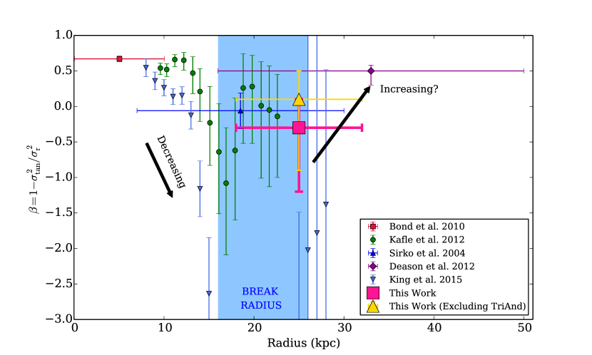
Figure 6.— Radial velocity anisotropy profile. The “break radius” of the Milky Way stellar halo is shown by the blue shaded region ($16\lesssim r/\rm{kpc}\lesssim 26$; Deason et al. 2011). Our measurement of $\beta$, from the 3D kinematics of $N=13$ stars in the radial range $18\lesssim r/\rm{kpc}\lesssim 32$, is shown in pink. Solar neighborhood measurements, using full 3D velocity information, find a radially biased $\beta$, shown in red (Bond et al. 2010; Smith et al. 2009). The remaining error bars show estimates of $\beta$ for distant ($D\gtrsim 10$ kpc) halo stars using LOS velocity distributions (Sirko et al. 2004; Kafle et al. 2012; Deason et al. 2012; King et al. 2015).

5. Discussion

Our value of $\beta$ is consistent with isotropy, and lower than local measurements by at least $1\sigma$, which find a radially biased anisotropy ($\beta=0.5-0.7$). The significant dispersion in the observed LOS velocity distribution (Figure 4) rules out the possibility that our sample is dominated by cold substructure.

Figure 6 shows the radial anisotropy profile of the Milky Way stellar halo. Our measurement is consistent with the observed “dip” in the anisotropy profile, seen in multiple studies that measured the velocity anisotropy of distant halo stars along different lines of sight using only LOS velocity distributions (Sirko et al. 2004; Kafle et al. 2012; Deason et al. 2012; King et al. 2015). This dip is also coincident with the observed break in the halo density profile around $16~{}\mbox{kpc}\lesssim r\lesssim 26~{}\mbox{kpc}$ (Deason et al. 2011; Sesar et al. 2011; Watkins et al. 2009). In this section, we discuss some of the possible explanations of this result.

5.1. A Galactic Shell

In D13, we argued that the presence of global substructure, such as a shell (or multiple shells), is one explanation for both the steep fall-off in stellar density beyond the break radius and the decrease in anisotropy at that radius. Deason et al. (2013a) argued that a break in the Milky Way stellar density profile could be created by the build-up of stars at apocenter from either one relatively massive accretion event or several, synchronous accretion events. In this scenario, we would expect the stars to have an increase in tangential motion relative to radial motion at the turnaround radius, and thus a more isotropic $\beta$, just as we observe. This picture is consistent with what we find for likely TriAnd members: TriAnd is a large, cloud-like overdensity of stars likely at apocenter (Johnston et al. 2012), and including TriAnd in our sample makes $\beta$ more tangentially biased. Chemical abundances for these stars may help to characterize the progenitor (or progenitors) of this shell (see Section 5.3.1).

Several of these cloud-like overdensities, such as TriAnd, the Virgo overdensity (VOD), the Hercules-Aquila overdensity (HerAq) and the Eridanus-Phoenix overdensity (EriPhe) are all located at approximately 20 kpc. Li et al. (2015) recently suggested that EriPhe, HerAq and the VOD could all be associated, and potentially fell in to the Milky Way as a group; TriAnd could also be a member of this group. A group infall event could explain the presence of all these overdensities at $\sim$ 20 kpc, the observed break in the density profile and the relative increase in tangential motion at this radius.

5.2. Dual Stellar Halo: In-Situ Star Formation

The break in the stellar density profile could also be an indication that the Milky Way has a “dual stellar halo,” containing populations of different origins (Carollo et al. 2007; Carollo et al. 2010; Beers et al. 2012). Simulations predict that the stellar halo is composed both of accreted stars and stars that form in-situ (e.g., Zolotov et al. 2009; Font et al. 2011; McCarthy et al. 2012; Tissera et al. 2012; Cooper et al. 2015). In-situ stars have two flavors. The first are stars that form in the halo itself from gas accreted from the IGM or satellites; it remains unknown to what extent these populations and their properties are a result of the choice of hydrodynamics scheme. Secondly, stars can form in the disk of the Milky Way and then be kicked up into the halo due to merger events (these stars are sometimes called “heated disk stars”). In simulations, these stars can comprise a significant fraction of the stellar population (and sometimes even dominate) within $r\lesssim 30$ kpc. It’s possible that our observed isotropy is a kinematic signature of a heated disk population. McCarthy et al. (2012) showed that these in-situ stars can have significant prograde rotation and therefore increased tangential pressure support from angular momentum, and we find a significant signal of prograde rotation ($\langle v_{\phi}\rangle\sim 70\ \mbox{km \ s}^{-1}$). However, this scenario does not explain why measurements of the velocity anisotropy in the solar neighborhood find radially biased orbits, in the region of the halo where we would expect even more heated disk stars. Distinguishing between accreted and in-situ populations with kinematics alone remains challenging, and model predictions remain unclear. To better determine if our objects were accreted or formed in-situ, we need chemical abundances (see Section 5.3.1).

5.3. Future Work

5.3.1 Chemistry

Chemical information is key for disentangling the Milky Way’s accretion history. Iron abundances of accreted populations are related to the masses of the dwarf progenitors (e.g., see Johnston et al. 2008; Kirby et al. 2013). If our 13 stars are accreted halo stars, measuring iron abundances may help to determine whether a single accretion event or several are responsible for the shell-type structure we observe, and we can use the abundances to estimate the mass(es) of the progenitor(s).

The chemical information in our stellar spectra is also our best hope of determining the relative contributions of different stellar halo formation mechanisms. Stars that form in the disk of the Milky Way in simulations are found to have a higher average [Fe/H] than accreted stars (Font et al. 2011; Tissera et al. 2012; Cooper et al. 2015). In addition, Zolotov et al. (2010) showed that in-situ stars are alpha-enriched relative to accreted stars at a given [Fe/H] at the high [Fe/H] end of the metallicity distribution function. These results are due to the fact that in-situ stars form in a deeper potential well than the accreted population. Several studies have used abundances in an effort to disentangle these populations locally (e.g. Nissen & Schuster (2010), with F and G main sequence stars within 335 pc; Sheffield et al. (2012) with M Giants out to 10 kpc). However, no such studies exist using main sequence stars outside the solar neighborhood. By measuring the iron and alpha abundances of distant main sequence halo stars, we can begin to assess the relative importance of different physical processes leading to the formation of the Milky Way’s stellar halo.

5.3.2 HALO7D

In order to better understand the global halo properties, we need more than $N\sim 13$ stars! Through the HALO7D observing program (begun in Spring 2014), we will obtain deep (8–24 hour integrations) spectra of hundreds of distant MSTO halo stars with measured HST proper motions using Keck II/DEIMOS. We will target $N\sim 350$ stars in the four CANDELS fields (Grogin et al. 2011; Koekemoer et al. 2011): GOODS-N, GOODS-S, COSMOS, and EGS. All four of these fields are characterized by deep, multi-epoch HST imaging, and cover a total area of approximately 1000 square arcminutes. With this dataset, we will:

1. Measure LOS velocities of all stars, as well as [Fe/H] and [$\alpha$/Fe] for those stars with sufficient signal to noise.

2. Measure the velocity anisotropy along four new lines of sight.

3. Measure the anisotropy as a function of galactocentric distance exclusively with stars that have 3D kinematic information.

4. Use chemical abundances to disentangle the Milky Way’s accretion history and determine the relative contributions of stellar halo formation mechanisms.

HALO7D is an ongoing observational program with results forthcoming (Cunningham et al., in prep).

6. Conclusions

We present line-of-sight (LOS) velocities for $N=13$ Milky Way halo stars with measured HST proper motions (PMs). Our sample is the first sample of halo stars with measured 3D kinematics outside of the solar neighborhood. The LOS velocities were measured from deep (5-6 hour) integrations on Keck II/DEIMOS. We combine the LOS velocity measurements with the proper motions to estimate the parameters of the velocity ellipsoid using an MCMC ensemble sampler. We find the velocity distribution in Galactic longitude l to have a mean $\langle v_{l}\rangle=-67^{+37}_{-37}\ \mbox{km \ s}^{-1}$ and a dispersion $\sigma_{l}=117^{+42}_{-20}\ \mbox{km \ s}^{-1}$. We find the dispersions in Galactic latitude b and the LOS to be $\sigma_{b}=88^{+28}_{-17}\ \mbox{km \ s}^{-1}$ and $\sigma_{\rm{LOS}}=91^{+27}_{-14}\ \mbox{km \ s}^{-1}$, respectively.

Using our estimates of the ellipsoid parameters, we measure the velocity anisotropy $\beta$. We find $\beta=-0.3^{+0.4}_{-0.9}$, consistent with isotropy and with the result from D13, but lower than solar neighborhood measurements, which find a radially biased $\beta$, by at least 1$\sigma$. If we exclude likely TriAnd members from our sample, we find $\beta=0.1^{+0.4}_{-0.9}$. These values are also consistent with other observational studies (using only LOS velocities) that have found a decrease in $\beta$ around the observed break radius in the Milky Way density profile ($16~{}\mbox{kpc}\lesssim r\lesssim 26~{}\mbox{kpc}$). These two findings in tandem suggest the presence of a shell-type structure in the halo at this radius, potentially formed by several destroyed dwarfs with similar apocenters. It is also possible that we are observing a population dominated by in-situ stars rather than an accreted population.

We need more observations and chemical information for distant halo stars to better understand the origin of the Milky Way stellar halo and its accretion history. We will achieve this with the HALO7D observing program, which will increase our sample of stars with 3D kinematics by a factor of $\sim$ 30. The velocities and abundances measured from these observations will vastly improve our understanding of the Galaxy’s accretion history and the origin of the stellar halo.

References

- Beers et al. (2012) Beers, T. C., Carollo, D., Ivezić, Ž., et al. 2012, ApJ, 746, 34
- Binney & Tremaine (2008) Binney, J., & Tremaine, S. 2008, Galactic Dynamics: Second Edition (Princeton University Press)
- Bond et al. (2010) Bond, N. A., Ivezić, Ž., Sesar, B., et al. 2010, ApJ, 716, 1
- Brown et al. (2004) Brown, T. M., Ferguson, H. C., Smith, E., et al. 2004, AJ, 127, 2738
- Brown et al. (2009) Brown, T. M., Smith, E., Ferguson, H. C., et al. 2009, ApJS, 184, 152
- Bullock & Johnston (2005) Bullock, J. S., & Johnston, K. V. 2005, ApJ, 635, 931
- Cappellari & Emsellem (2004) Cappellari, M., & Emsellem, E. 2004, PASP, 116, 138
- Carollo et al. (2007) Carollo, D., Beers, T. C., Lee, Y. S., et al. 2007, Nature, 450, 1020
- Carollo et al. (2010) Carollo, D., Beers, T. C., Chiba, M., et al. 2010, ApJ, 712, 692
- Cooper et al. (2015) Cooper, A. P., Parry, O. H., Lowing, B., Cole, S., & Frenk, C. 2015, MNRAS, 454, 3185
- Cooper et al. (2010) Cooper, A. P., Cole, S., Frenk, C. S., et al. 2010, MNRAS, 406, 744
- Cooper et al. (2012) Cooper, M. C., Newman, J. A., Davis, M., Finkbeiner, D. P., & Gerke, B. F. 2012, spec2d: DEEP2 DEIMOS Spectral Pipeline, Astrophysics Source Code Library, ascl:1203.003
- Deason et al. (2011) Deason, A. J., Belokurov, V., & Evans, N. W. 2011, MNRAS, 416, 2903
- Deason et al. (2012) Deason, A. J., Belokurov, V., Evans, N. W., & An, J. 2012, MNRAS: Letters, 424, L44
- Deason et al. (2013a) Deason, A. J., Belokurov, V., Evans, N. W., & Johnston, K. V. 2013a, ApJ, 763, 113
- Deason et al. (2013b) Deason, A. J., Van der Marel, R. P., Guhathakurta, P., Sohn, S. T., & Brown, T. M. 2013b, ApJ, 766, 24 (D13)
- Deason et al. (2014) Deason, A. J., Belokurov, V., Hamren, K. M., et al. 2014, MNRAS, 444, 3975
- Faber et al. (2003) Faber, S. M., Phillips, A. C., Kibrick, R. I., et al. 2003, in Society of Photo-Optical Instrumentation Engineers (SPIE) Conference Series, Vol. 4841, Instrument Design and Performance for Optical/Infrared Ground-based Telescopes, ed. M. Iye & A. F. M. Moorwood, 1657–1669
- Font et al. (2011) Font, A. S., McCarthy, I. G., Crain, R. A., et al. 2011, MNRAS, 416, 2802
- Foreman-Mackey et al. (2013) Foreman-Mackey, D., Hogg, D. W., Lang, D., & Goodman, J. 2013, PASP, 125, 306
- Foreman-Mackey et al. (2014) Foreman-Mackey, D., Price-Whelan, A., Ryan, G., et al. 2014, triangle.py v0.1.1, doi:10.5281/zenodo.11020
- Goodman & Weare (2010) Goodman, J., & Weare, J. 2010, Communications in Applied Mathematics and Computational Science, 5, 65
- Grogin et al. (2011) Grogin, N. A., Kocevski, D. D., Faber, S. M., et al. 2011, ApJS, 197, 35
- Jeffery et al. (2011) Jeffery, E. J., Smith, E., Brown, T. M., et al. 2011, AJ, 141, 171
- Johnston et al. (2008) Johnston, K. V., Bullock, J. S., Sharma, S., et al. 2008, ApJ, 689, 936
- Johnston et al. (2012) Johnston, K. V., Sheffield, A. A., Majewski, S. R., Sharma, S., & Rocha-Pinto, H. J. 2012, ApJ, 760, 95
- Kafle et al. (2012) Kafle, P. R., Sharma, S., Lewis, G. F., & Bland-Hawthorn, J. 2012, ApJ, 761, 98
- Kalirai (2012) Kalirai, J. S. 2012, Nature, 486, 90
- King et al. (2015) King, III, C., Brown, W. R., Geller, M. J., & Kenyon, S. J. 2015, ArXiv e-prints, arXiv:1506.05369
- Kirby et al. (2013) Kirby, E. N., Cohen, J. G., Guhathakurta, P., et al. 2013, ApJ, 779, 102
- Koekemoer et al. (2011) Koekemoer, A. M., Faber, S. M., Ferguson, H. C., et al. 2011, ApJS, 197, 36
- Li et al. (2015) Li, T. S., Balbinot, E., Mondrik, N., et al. 2015, ArXiv e-prints, arXiv:1509.04296
- Martin et al. (2014) Martin, N. F., Ibata, R. A., Rich, R. M., et al. 2014, ApJ, 787, 19
- McCarthy et al. (2012) McCarthy, I. G., Font, A. S., Crain, R. A., et al. 2012, MNRAS, 420, 2245
- McMillan (2011) McMillan, P. J. 2011, MNRAS, 414, 2446
- Naab et al. (2006) Naab, T., Khochfar, S., & Burkert, A. 2006, ApJ, 636, L81
- Nissen & Schuster (2010) Nissen, P. E., & Schuster, W. J. 2010, A&A, 511, L10
- Reid et al. (2009) Reid, M. J., Menten, K. M., Zheng, X. W., et al. 2009, ApJ, 700, 137
- Schönrich (2012) Schönrich, R. 2012, MNRAS, 427, 274
- Schönrich et al. (2010) Schönrich, R., Binney, J., & Dehnen, W. 2010, MNRAS, 403, 1829
- Sesar et al. (2011) Sesar, B., Jurić, M., & Ivezić, Ž. 2011, ApJ, 731, 4
- Sheffield et al. (2014) Sheffield, A. A., Johnston, K. V., Majewski, S. R., et al. 2014, ApJ, 793, 62
- Sheffield et al. (2012) Sheffield, A. A., Majewski, S. R., Johnston, K. V., et al. 2012, ApJ, 761, 161
- Sirko et al. (2004) Sirko, E., Goodman, J., Knapp, G. R., et al. 2004, AJ, 127, 914
- Smith et al. (2009) Smith, M. C., Evans, N. W., Belokurov, V., et al. 2009, MNRAS, 399, 1223
- Sohn et al. (2012) Sohn, S. T., Anderson, J., & van der Marel, R. P. 2012, ApJ, 753, 7
- Tissera et al. (2012) Tissera, P. B., White, S. D. M., & Scannapieco, C. 2012, MNRAS, 420, 255
- VandenBerg et al. (2006) VandenBerg, D. A., Bergbusch, P. A., & Dowler, P. D. 2006, ApJS, 162, 375
- Watkins et al. (2009) Watkins, L. L., Evans, N. W., Belokurov, V., et al. 2009, MNRAS, 398, 1757
- Xue et al. (2008) Xue, X. X., Rix, H. W., Zhao, G., et al. 2008, ApJ, 684, 1143
- Zolotov et al. (2009) Zolotov, A., Willman, B., Brooks, A. M., et al. 2009, ApJ, 702, 1058
- Zolotov et al. (2010) Zolotov, A., Willman, B., Brooks, A. M., et al. 2010, ApJ, 721, 738