Finding the
effective structure parameters for
suspensions of nano-sized
insulating particles from low-frequency impedance measurements
111 author, e-mail: mrs@onu.edu.ua, V. Ya. , and M. V.
of Theoretical Physics, Mechnikov National University
of General and Chemical Physics, Mechnikov National University
2 Dvoryanska St., Odesa 65026, Ukraine
Abstract
Based on the method of compact groups of inhomogeneities, we formulate new mixing rules for suspensions of charged insulating particles. They express the quasistatic conductivity and permittivity of a suspension in terms of the effective geometric and dielectric parameters of the particles, electric double layers (EDLs), and suspending liquid. Also, we present our low-frequency impedance measurements of the conductivity and permittivity of -isopropyl alcohol nanofluids as functions of -particle volume concentration. Our rules give good fits for most of these data and allow us to estimate, among other things, the effective thickness, conductivity, and permittivity of the EDLs. The experimentally-recovered values agree well with elementary theoretical estimates suggesting the charging of the particles through preferential adsorption of contaminant ions. The possible effects of other mechanisms on the effective conductivity and permittivity of suspensions are also discussed.
Keywords: Electrical conductivity, Permittivity, Suspension, Nanofluid, Electric double layer, Compact group method, Impedance spectroscopy
1 Introduction
The nature and structure of interphase layers in dispersions and nanofluids (liquid-based suspensions of nano-sized particles) have been under intensive study in the context of their effect on various bulk properties of the entire system. In particular, it is recognized that the diffuse electrical double layers (EDLs) play an essential role in the formation of the conductivity and permittivity of nanofluids [1, 2, 3, 4, 5, 6, 7]. However, the details of pertinent mechanisms and their incorporating into a consistent quantitative theory of the effective electrical properties of nanofluids still remain to be investigated. For example, the classical Maxwell–Garnett [8, 9] and Bruggemann [10] mixing rules fail to explain a dramatic enhancement of upon addition of small amounts of insulating nanoparticles. The reasons are that they, first, ignore the actual microstructure of the system and, second, are one-particle approximations. Modern approaches (see [1, 2, 3, 4, 5, 6, 7]) to the problem represent various sophisticated modifications of the electrokinetic theories [11, 12, 13, 14] and deal with a set of coupled differential equations for the flow field and for quantities related to the ion density and electric field distributions around a hard particle. The results heavily depend on model assumptions about the factors and mechanisms responsible for the formation of these distributions and are usually restricted to situations where the total volume concentration of the particles and their EDLs is very small. The latter means that the electromagnetic interactions between the structural inhomogeneities, formed by the particles and their EDLs, are weak, so that finding the effective conductivity and permittivity of the entire suspension is actually reduced to finding those of a single inhomogeneity and then corrections to them in the lowest orders of various perturbation techniques. Most known attempts at analyzing the effective parameters of concentrated suspensions are based upon Happel’s [15] and Kuwabara’s [16] cell models. On the outer surface of the unit cell, the governing electrokinetic equations are subject to certain boundary conditions of the Neumann or Dirichlet type. Being supposed to account for the averaged effects of the surrounding medium on the cell, the boundary conditions are constructed by applying mean-field considerations to the local fields (see [17, 18, 19, 20, 21, 22, 23, 24] and references therein). This is equivalent, once again, to the assumption that the properties of a suspension are derived from those of a single cell placed in a uniform and isotropic host medium.
The major points of this report are as follows.
First, we outline a new approach to the effective electrical properties of nanofluids which is based upon the method of compact groups of inhomogeneities [25, 27, 26, 28]. Within the latter, the nanofluid’s microstructure is modelled in terms of the complex permittivity profiles of the constitutients. The desired conductivity and permittivity are expressed in terms of the moments of these profiles and the volume concentrations of the constitutients. The moments themselves can be evaluated without a detailed elaboration of many-particle polarization and correlation processes in the system. In particular, we present our theoretical results for a system of hard-core-penetrable-shell particles embedded into a uniform matrix. The further attention is focused on the situation where the core radius , the shell thickness , and the Debye length are comparable: .
Second, we present the results of our experimental studies of the quasistatic conductivity and permittivity of -isopropyl alcohol nanofluids as functions of -particle volume concentration . The electrical parameters of the base liquid (isopropyl alcohol, IPA) samples were typical of industrial samples, for the purity requirements to the base liquid were not mandatory for our purposes. In contrast, we took advantage of the presence of contaminant ions in the samples to make simple physical estimates in support of our model, as shown later.
Finally, we use our theory to process the experimental data obtained. We show that the observed behavior of and can directly be interpreted as a result of formation of EDLs around the nanoparticles and evaluate the parameters of these layers.
2 Theoretical Background
2.1 General Equations
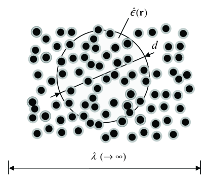
Suppose that the wavelength of probing radiation is much longer than typical distances between the particles dispersed in a continuous medium. The dielectric response of such a system can effectively be treated by the method of compact groups of inhomogeneities [25, 27]. These groups are defined as macroscopic regions within which all the distances between the particles are much shorter than . With respect to a probing field with , such groups are actually point-like inhomogeneities, but yet include sufficiently large numbers of particles to reproduce the properties of the entire system. Under these conditions, a system can be viewed as a set of compact groups and characterized by a certain (modeled according to the system’s microstructure) profile of its complex permittivity. Using methods of the theory of generalized functions [29] and a special representation [30, 31] for the electromagnetic field propagator, we can, first, extract the leading compact groups’ contributions to the averaged field and induction in the system without modeling multiple reemission and short-range correlation effects in depth and, second, prove that it is these contributions that form the quasistatic dielectric and conductive properties of the system. Eventually, the problem reduces to calculating and summing up the moments of the complex permittivity profile within the system; the size of compact groups, because of their macroscopicity, turns out to be an insignificant parameter. In application to suspensions (see Fig. 1), the essential details of the compact-group approach are as follows.
We determine the quasistatic complex permittivity of a suspension as the proportionality coefficient in the relation [32]
| (1) |
where
| (2) |
is the local complex permittivity value in the suspension, is the electric constant, and the angular brackets stand for the ensemble averaging or averaging by integration over the volume. Expression (2) suggests that the effective response of the suspension to a probing field is equivalent to that of an imaginary system made up by embedding the suspension’s constituents, including the base liquid, into a host having a complex permittivity . The response of this imaginary system is formed by multiple reemissions and correlations within compact groups of its constituents (dispersed particles and regions filled with the suspending liquid). Then the averaged field and induction are given by
| (3) |
| (4) |
where is the probing field amplitude in the host of permittivity .
Henceforth, we take to be equal to the looked-for permittivity . This choice implies the use of the Bruggeman-type of electrodynamic homogenization, which, however, is not identical to the classical Bruggeman (mean-field) approach [10]; the latter considers only the responses of solitary particles to a uniform effective field [33]. Then, for a suspension of identical particles consisting of hard cores (with radius and permittivity ) and concentric penetrable shells (with outer radius and permittivity ) and embedded in a suspending liquid (with permittivity ), the moments of are
| (5) |
where (), is the volume concentration of the hard cores, and is that of the core-shell particles; is the relative thickness of the shells. In view of (5), the series (3) and (4) can be summed up. The substitution of the sums into (1) gives the equation for :
| (6) |
Modeling the complex permittivities of the constituents as and the effective complex permittivity as , we can distinguish different types of the system’s response to an external probing radiation of angular frequency . In what follows, we consider the situation which occurs in the limiting case . Then (6) reduces to two real equations, of which the governing equation is that for :
| (7) |
After it is solved, is found from the linear equation
| (8) |
The criterion of applicability of (7) and (8) is conveniently represented as
| (9) |
where and are expressed in and is the linear frequency of probing radiation in . It follows from the requirement that , which is expected to hold true for sufficiently small and is used to derive (7) and (8) from (6) within a perturbation scheme with respect to .
The details of the proof of (5)–(8) for the case where the averaging procedure is reduced to direct integration over the region occupied be the suspension can be found in [28]; the proof within the statistical ensemble averaging will be published elsewhere. It can also be proven that it is the Bruggeman-type of electrodynamic homogenization (as described above) that is compatible with the compact-group approach.
2.2 Maxwell–Garnett rule
The conductive properties of diluted suspensions are often treated with the Maxwell–Garnet rule [8, 9]
| (10) |
To substantiate it, one usually assumes that the dispersed particles are distributed randomly, their volume concentration is low, the interaction between them is negligibly small, and only the contributions from their induced electric dipoles are of significance. Nonetheless, (10) is sometimes used to describe suspensions with high particle concentrations [34, 35, 36], where the mutual polarization and correlation effects of higher orders come into play. The effect of the interphase is ignored in deriving (10).
It should be noted that the Maxwell–Garnett rule can be obtained within the compact-group approach under the suggestions that the suspending liquid is taken as the host matrix for electrodynamic homogenization () and the dispersed hard particles have no outer shells. The details of relevant calculations can be found in [25, 26, 27].
When applying (10) in practice, three limiting representations of it for can be useful (see, for instance, [36]), depending on the relative magnitude of the particle conductivity, as compared to the suspending liquid conductivity. Introducing the relative magnitude of the suspension conductivity, we have:
(A) If (insulating particles), then
| (11) |
(B) If (highly conducting particles), then
| (12) |
(C) If , then
| (13) |
These limiting laws are indeed observed in experiment [34, 36, 37], as well as deviations from them [37, 38]. In particular, if the volume concentration of the dispersed particles is increased to values of order 0.05, then, according to these rules, the conductivity of a suspension of insulating particles is expected to decrease by 8% and that of highly conducting particles to increase by no more than 15%. However, experiment reveals that in both cases the nanofluid conductivity can increase by one or even two orders in magnitude (see recent works [39, 40, 41, 42, 43, 44, 45] and references therein). Qualitatively, these deviations are explained by a complex microstructure of suspensions – first of all, by the formation of EDLs around the particles. Since the Maxwell–Garnett rule lacks any EDL parameters, it fails to give any quantitative estimates of them and predict their effect on ; neither can it explain a strong enhancement of with .
2.3 New Rules For Suspensions of Insulating Particles
Now, we use (7) to analyze the important case of suspensions of insulating particles. Despite the fact that this equation is based upon the Bruggeman-type of electrodynamic homogenization, it not only reduces, under appropriate assumptions, to the Maxwell–Garnett limiting laws (11)–(13), but also can account for possible deviations from them as functions of the effective parameters of the interphase.
In (7), the interphase is characterized by the conductivity (or relative conductivity , as compared to the suspending liquid conductivity) and the net volume concentration . For spherical hard-core-penetrable-shell particles, their effective volume concentration , where is the relative thickness of the shell (as compared to the hard-core radius). The estimates for are available in literature. In particular, it has been shown that the analytical scaled-particle approximation result [46]
| (14) |
is in very good agreement with the Monte Carlo simulation results [47, 48]
| (15) |
In what follows, we use estimate (14). In the limit of diluted suspensions (), all above results take the form
| (16) |
For hard particles with no shells and , and for core-shell particles . If and , then . The dependence of the shell volume concentration upon for several is shown in Fig. 2.

For insulating particles, , (7) reduces to the quadratic equation
| (17) |
Simple algebraic manipulations immediately give:
(1) If , then
| (18) |
(2) If , then
| (19) |
(3) If , then
| (20) |
For diluted suspensions with thin particle shells (, , ) and , the limiting rules (18)–(20) reduce to the Maxwell–Garnet liming rule (11). As increases, deviations from (11) appear. The greater , the greater they are for a given . As increases, they also increase.
As already noted, the effective conductivity of nanofluids can increase by up two orders of magnitude as the volume concentration of embedded insulating nanoparticles increases by a few percent only. Such behavior is in drastic disagreement with the Maxwell–Garnett rule (10) and its limiting representations (11)–(13). On the contrary, rule (17) can potentially explain this behavior, as seen from its limiting representation (20). Two, at least, factors are essential for this: the presence of sufficiently thick interphase layers between the particles and the suspending liquid; a relatively high conductivity of these layers. A positive conductivity increment is expected for layers with , where the threshold value is, according to (20), the solution of the equation . Using (16) and the approximate formula , , gives . Consequently, the conductivity is expected to increase with for suspensions with parameter . Under the suggestion that , this estimate agrees well with the conductivity results [49], especially those derived from the electrophoretic mobility measurements, for colloids of polystyrene latex particles.
It should be emphasized that electrophoretic measurements deal with the motion of a practically solitary particle; the redistribution of ions near it due to its acquired charge does not affect the background ionic strength. On the other hand, direct electrical conductivity measurements deal with averaged properties of a suspension comprising a small, but finite number of particles; when charged, these particles can alter the concentrations of ions in regions both inside and outside the EDLs (in particular, due to nonspecific adsorption [50]).
Equation (17) can be used for finding the effective parameters of suspensions of insulating particles from low-frequency impedance measurements. Its physically meaningful solution is
| (21) |
As found above, the asymptotics of at and are given by (18) and (20), respectively, with missing. For diluted suspensions with , (21) simplifies to
| (22) |
With formula (21) available, we can estimate , together with , by fitting experimental data for . An additional opportunity is opened by equation (8), from which the effective permittivity of suspensions of insulating particles
| (23) |
where and . The second term in the numerator can be neglected (the dependence of on can be ignored) if and .
3 Experiment
3.1 Samples and Measurements’ Details
Two series of nanofluid samples were studied. They were prepared by the ultrasonic dispersing of particles with passport size of in base liquid (isopropyl alcohol, IPA) followed by long-term settling and sedimentation of large particles. The starting mass fraction of particles in the stable nanofluids was . The size control, with dynamic light scattering, revealed that the dispersed phase consisted of single uncoagulated particles with approximately equal radii. The samples of different concentrations were prepared by diluting the initial nanofluid sample with the base liquid. The mass fraction values for all samples were determined by the analytical weighing of the net mass of the particles left after the suspending liquid was evaporated. The volume concentrations were recovered via the particle mass fractions by
where the base liquid density and particle density were taken to be and , respectively.
The nanofluid conductivity and permittivity were measured as functions of using an impedance test cell. It consisted of two rectangular platinum electrodes, with dimensions and 3 mm apart, placed in a container with nanofluid samples, of a -volume each. The impedance data were taken with a Soviet-made automatic digital bridge device E7-8 at a frequency of kHz for ranging from 0.0035 to 0.049 at C. This device depends for its operation on the bridge method with phase-sensitive detectors for bridge balancing and is designed to measure the electrical impedance of both two-terminal and multi-branch networks. It also enables impedance measurements with a bias voltage/current applied to the sample. We used the operating mode for measuring the impedance of two-terminal configurations with their equivalent circuits being the active resistance and capacitance in parallel. In this mode, the device measurement limits for conductance and capacitance were 0.1 nS to 1 S and 0.01 pF to 100 , respectively. The instrumental uncertainty was of full scale + 1 digit.
It was taken into account that considerable measurement errors could be introduced by the polarization at the interface between the electrodes and the sample, especially when the low-frequency permittivity of the sample was measured. In the impedance cell, the electrode polarization impedance was in series with the sample impedance , so that the total impedance . We measured with the bridge method; in terms of an equivalent parallel combination, where and are the measured resistance and capacitance, respectively. The use of platinum electrodes was expected to reduce by several orders of magnitude. The remaining distorting effect of the electrode polarization was estimated by the formulas [56, 57]
| (24) |
Using the latter one and contrasting our experimental data for IPA with literature data, we found that at most. We believe that the actual value of was in our experiment several times smaller. Under the suggestion , we recovered with (24) the and data and then the conductivities and permittivities of the nanofluid samples.
The lowest values of and achieved by dilution of the nanofluid samples were, respectively, and 37.2 for series I and and for series II (see Table 1). These values are higher than those known for pure IPA, and at room temperatures [51], but correlate well with the conductivity value of at C, reported in [52] for IPA samples recycled after spending. The conductivity and permittivity of our IPA samples were measured to be and 28.25, respectively. The former correlates with data [53], according to which the IPA conductivity is at C.
Table 1. Parameters of most diluted nanofluids
| Series | |||
|---|---|---|---|
| I, 34 samples | 0.0042 | 0.70 | 37.2 |
| II, 47 samples | 0.0035 | 1.05 | 34.4 |
3.2 Experimental Results and Their Processing
Table 2. Data Fitting Results
| series | |||||
|---|---|---|---|---|---|
| I | 1.17 | 35 | 0.90 | 35 | 65 |
| II | 1.68 | 12 | 1.21 | 12 | 12 |
The measurement results for and , normalized by their values and for the most diluted nanofluid samples with the nanoparticle concentrations (see Table 1), and the fits to these data with the formulas
| (25) |
| (26) |
(which enable us to reduce the number of fitting parameters to two and three, respectively) are represented in Figs. 3 and 4; the best values of the fitting parameters are summarized in Table 2. In the next section, we show that most of these values can be recovered within an elementary model suggesting that the nanoparticles acquire charge upon dispersing them in base liquid; this leads to the formation of EDLs around them and alters the bulk ion concentration in the suspending liquid. The variations in the relative thickness (at a fixed relative conductivity ) of EDLs within each series of the and data may be due to the fact that we ignore the spatial inhomogeneity of EDLs.
The internal consistency of the fitting results was also verified with the formula
| (27) |
which follows from (17). Note that (27) can be convenient to attack the inverse problem of recovering and from the experimental versus dependence.


4 Some Estimates and Considerations
Suppose that the conductivity of our base liquid is mainly due to ionic contamination of pure IPA with ions having unit charges (of both signs) and equal mobilities . The total concentration of these ions . Next, assume that after being dispersed into this liquid, particles become like-charged, their acquired charges residing on their surfaces. Via the Coulomb force, these surface charges cause the formation of concentric diffuse layers of ions around the particles. Because the total number of dispersed particles , the total number of ions on their surfaces ; the latter is equal, in view of the electroneutrality condition, to the total number of the excess counterions within the diffuse layers. Here, is the volume of the nanofluid sample and is that of each particle. The appearance of the surface- and diffuse-layer-bound ions reduces the concentration of free ions associated with the suspending liquid to and, consequently, the conductivity of this liquid to . For sufficiently small (though finite) , can be equated to the measured nanofluid conductivity . Taking , , and , we obtain the estimate for the particle charge number in the most diluted nanofluid of sample series II. Having the measured permittivity of this nanofluid, we further find that the Debye length and the ratio . The average concentration of the excess counterions in each diffuse layer where is the volume of the layer. The relative conductivity of the layers can be evaluated as . For , we obtain and . In the case of sample series I, , and . For , we find that and . Lastly, we note that for both sample series; this is considerably greater than (series I) and (series II). Evaluating as ( is the limiting ionic conductivity and is Avogadro’s number) and taking for typical literature values of and , we obtain and , respectively. These are very close to the experimentally-recovered values, given by . The estimates by and with the same ’s give, rather satisfactorily, (series I) and (series II).
Despite their simplicity, the above estimates are internally consistent and agree sufficiently well with our data processing results. This fact is a strong argument for the model being proposed. In this respect, several more points are worth noting.
First, our experimental curves in Figs. 3, 4 exhibit pronounced curvatures. Provided , similar behavior is revealed by the versus curves for latex suspensions which were first exhaustively ion-exchanged and then dialyzed against deionized water for 24 to 48 h [49]; no curvature was observed in latex suspensions which had been cleaned extensively by ion exchange. As pointed out in [49], these facts indicate a high sensitivity of to ionic contamination. Quantitative cell-model-based estimates [58] for the effect of atmospheric contamination on of aqueous salt-free suspensions lead to similar conclusions. In view of [58], the formation of a plateau-like segment on the experimental versus dependence in Fig. 3 b, where our theory and experiment deviate most, may result from a higher-than-expected level of uncontrolled contamination for sample series I. If so, the variations in the numerical values of the fitting parameters for the two sample series are reasonably explicable.
Second, assuming that the particles acquire charge by adsorbing contaminant ions, we can explain the initial decrease of at very small by depletion of the base liquid in those ions. As increases further, the particles’ conducting EDLs may begin to form percolation-type paths. This effect (most likely, enhanced by others, such as dissociation of base liquid, Donnan exclusion [3] etc.) should cause and to start increasing with . The conductivity increment sign reversal has indeed been observed in suspensions with low ionic strength (see, for instance, [49, 45]).
Third, as the graphs in Fig.5 reveal, our model predicts that at higher , when the overlapping of EDLs comes into play, the rate of growth, , of and that of may decrease, reach zero levels, and even become negative. Such trends have been observed for , but at lower (see, for instance, [40, 41, 42, 59]). For a salt-free medium, the decrease of with can be explained [41] by counterion condensation [60, 61, 62] near the particles which develop high surface charge due to the protonation or deprotonation of surface groups. In terms of our model, this mechanism can be accounted for through, at least, the reduction of the effective thickness of EDLs without changing the conductivity outside. On the other hand, if the charging of particles occurs mainly through preferential adsorption of contaminant ions, then the bulk ion concentration should decrease with and the effective should increase. Consequently, the indicated scenario for is expected at lower values of , compared to those shown in Fig. 5 (see also Fig. 2).
Finally, in view of our estimate , it might be suggested that the -behavior of in our model should resemble that predicted by the electrokinetic theory [61, 62] for dilute suspensions of spherical particles in a salt-free medium containing counterions only. Based upon Kuwabara’s cell model and arguments [63], Ohshima showed that if the total surface charge of the particle exceeds a critical value given, for univalent counterions, by
where is the relative permittivity of the medium, is the Boltzmann constant, and is the absolute temperature, then the counterion concentration takes a practically constant value
except in the region very near the particle surface. Correspondingly [61, 41], the suspension conductivity is
and parameter (25) becomes
Taking , and the previous values for the other parameters, for we find and, consequently, , (series I) and , (series II). As expected, these values are considerably smaller than those for our samples. Simultaneously, as a function of reveals an increase of the same order as does (see Fig. 5 a). It is also seen that the initial segments of these graphs have different curvatures. In our opinion, this fact is indicative of different nature of the models considered: the cell model is a mean-field approach, while ours is a percolation-type theory, with the effective microstructure parameters , and .
5 Conclusion
The main results of this report can be summarized as follows. The general expressions for the quasistatic effective electrical conductivity and permittivity of systems of hard-core-penetrable-shell particles, obtained earlier with the method of compact groups of inhomogeneities, have been scrutinized to formulate new mixing rules for suspensions of charged insulating particles. These rules express the conductivity and permittivity of a suspension in terms of the effective geometric and dielectric parameters of its constituents (the particles, their EDLs, and the suspending liquid). They effectively incorporate higher-order correlations and polarizations in the suspension without in-depth modeling these processes. Thus the problem of electrodynamic homogenization of a suspension is reduced to a simpler problem of finding the effective parameters of its constituents; the latter can be attacked with, say, the standard electrokinetic theory. On the other hand, the rules obtained can be used to extract the effective parameters of the constituents from low-frequency impedance measurements.
Such measurements have been done for two series of -isopropyl alcohol nanofluids to obtain their conductivity and permittivity as functions of -particle volume concentration. The functional form of the new rules is sufficient to fit these dependences even under simplest suggestions about the mechanism of charging of the particles and its impact on the system. In particular, the recovered values of the parameters agree well with elementary theoretical estimates based on the idea that the particles acquire charges through preferential adsorption of contaminant ions. The possible effects of other mechanisms on the effective conductivity and permittivity of suspensions are also discussed.
We hope that our results will stimulate further studies in the field, including the performance of specially-designed experiments.
Acknowledgements
This research was supported in part by Ministry of Education and Science of Ukraine through Grant 0113U001377. We also thank Prof. D.K. Das and Dr. S. Sikdar for providing copies of their articles.
References
- [1] S.S. Dukhin, B.V. Derjaguin, Electrokinetic Phenomena, in: Surface and Colloid Science, E. Matijević (Ed.), Vol. 7, John Wiley, New York, 1974, Chap. 2.
- [2] R.J. Hunter, Zeta Potential in Colloid Science. Principles and Applications, Academic Press, London, 1981.
- [3] J. Lyklema, Fundamentals of Interface and Colloid Science, Vol II: Solid-Liquid Interfaces, Academic Press, London, 1995, Chaps. 3, 4.
- [4] R.J. Hunter, Foundations of Colloid Science, 2nd ed., Oxford University Press, Oxford, 2001, Chaps. 7, 8.
- [5] H. Morgan, N.G. Green, AC Electrokinetics: Colloids and Nanoparticles, Research Studies Press Ltd., Baldock, Hertfordshire, England, 2003.
- [6] A.V. Delgado et al. Measurement and Interpretation of Electrokinetic Phenomena (IUPAC Technical Report), Pure Appl. Chem. 77 (2005) 1753.
- [7] H. Ohshima (Ed.), Electrical Phenomena at Interfaces and Biointerfaces. Fundamentals and Applications in Nano-, Bio-, and Environmental Sciences, John Wiley & Sons, Hoboken, New Jersey, 2012.
- [8] J.C. Maxwell, A Treatise on Electricity and Magnetism, Vol. 1, 1st ed., Clarendon Press, Oxford, 1873, pp. 362–365.
- [9] J.C.M. Garnett, Phil. Trans. R. Soc. Lond. A 203 (1904) 385.
- [10] D.A.G. Bruggeman, Ann. Phys. (Leipzig) 24 (1935) 636.
- [11] R.W. O’Brien, L.E. White, J. Chem. Soc. Faraday Trans. II 74 (1978) 1607.
- [12] D.A. Saville, J. Colloid Interface Sci. 71 (1979) 477.
- [13] R.W. O’Brien, J. Colloid Interface Sci. 81 (1981) 234.
- [14] E.H.B. DeLacey, L.R. White, J. Chem. Soc. Faraday Trans. II 77 (1981) 2007.
- [15] J. Happel, Am. Inst. Chem. Eng. J. 4 (1958) 197.
- [16] S. Kuwabara, J. Phys Soc. Jpn 14 (1959) 527.
- [17] S. Levine, G.H. Neale, J. Colloid Interface Sci. 47 (1974) 520.
- [18] S. Levine, G.H. Neale, N. Epstein, J. Colloid Interface Sci. 57 (1976) 424.
- [19] M.W. Kozak, E.J. Davis, J. Colloid Interface Sci. 127 (1989) 497.
- [20] M.W. Kozak, E.J. Davis, J. Colloid Interface Sci. 129 (1989) 166.
- [21] H. Ohshima, J. Colloid Interface Sci. 188 (1997) 481.
- [22] H. Ohshima, J. Colloid Interface Sci. 212 (1999) 443.
- [23] J. Cuquejo et al., J. Phys. Chem. B 110 (2006) 6.
- [24] F. Carrique, E. Ruiz-Reina, F.J. Arroyo, Â. V. Delgado, J. Phys. Chem. B 110 (2006) 18313.
- [25] M.Ya. Sushko, Zh. Eksp. Teor. Fiz. 132 (2007) 478; JETP 105 (2007) 426.
- [26] M.Ya. Sushko, S.K. Kris’kiv, Zh. Tekh. Fiz. 79 (2009) 97; Tech. Phys. 54 (2009) 423.
- [27] M.Ya. Sushko, J. Phys. D: Appl. Phys. 42 (2009) 155410.
- [28] M.Ya. Sushko, A.K. Semenov, Condens. Matter Phys. 16 (2013) 13401.
- [29] V.S. Vladimirov, Equations of Mathematical Physics, 3rd ed., Nauka, Moscow, 1981; Marcel Dekker, New York, 1971.
- [30] W. Weiglhofer, Am. J. Phys., 57 (1989) 455.
- [31] M.Ya. Sushko, Zh. Eksp. Teor. Fiz. 126 (2004) 1355; JETP 99 (2004) 1183.
- [32] L.D. Landau, E.M. Lifshitz, L.P. Pitaevskii, Course of Theoretical Physics, Vol. 8: Electrodynamics of Continuous Media, 2nd ed., Nauka, Moscow, 1982; Pergamon, Oxford, 1984.
- [33] D.J. Bergman, D. Stroud, Sol. State Phys. 46 (1992) 147.
- [34] J.C.R. Turner, Chem. Eng. Sci. 31 (1976) 487.
- [35] R. Barchini, D.A. Saville, J. Colloid Interface Sci. 173 (1995) 86.
- [36] R.C.D. Cruz et al., J. Colloid Interface Sci. 286 (2005) 579.
- [37] R.E. Meredith, C.W. Tobias, J. Electrochem. Soc. 108 (1961) 286.
- [38] R.E. De La Rue, C.W. Tobias, J. Electrochem. Soc. 106 (1959) 827.
- [39] S. Ganguly, S. Sikdar, S. Basu, Powder Technol. 196 (2009) 326.
- [40] J.D. Posner, Mechanics Research Comm. 36 (2009) 22.
- [41] S.B. White, A.J.-M. Shih, K.P. Pipe, Nanoscale Research Lett. 6 (2011) 346.
- [42] S. Sikdar, S. Basu, S. Ganguly, Int J. Nanoparticles 4 (2011) 336.
- [43] H. Konakanchi, R. Vajjha, D. Misra, D. Das, J. Nanosci. Nanotechnol. 11 (2011) 6788.
- [44] A.A. Minea, R.S. Luciu, Microfluid Nanofluid 13 (2012) 977.
- [45] K.G.K. Sarojini et al., Colloids and Surfaces A: Physicochem. Eng. Aspects 417 (2013) 39.
- [46] P.A. Rikvold, G. Stell, J. Chem. Phys. 82 (1985) 1014; J. Colloid Interface Sci. 108 (1985) 158.
- [47] S.B. Lee, S. Torquato, J. Chem. Phys. 89 (1988) 3258.
- [48] M. Rottereau, J. Gimel, T. Nicolai, D. Duran, Eur. Phys. J. E 11 (2003) 61.
- [49] C.F. Zukoski IV, D.A. Saville, J. Colloid Interface Sci. 107 (1985) 322.
- [50] D.A. Saville, J. Colloid Interface Sci. 91 (1983) 34.
- [51] Shell Chemicals, Data Sheet, Isopropyl Alcohol, September 2009, p. 2; LabChem, Safety Data Sheet, Isopropyl Alcohol (2-Propanol), November 2013, p. 5; Johann Haltermann Ltd, Technical Data & Safety Bulletin, Isopropyl Alcohol (IPA), July 2012, p. 2.
- [52] B.A. Donahue, A.R. Tarrer, S. Dharmawaram, S.B. Joshi, Used Solvent Testing and Reclamation, Volume II: Vapor Degreasing and Precision Cleaning Solvents, USA–CERL Technical Report N–89/03, Vol. II and AFESC Report ESL–TR–88–03, AD–A204 732, NTIS, Springfield, VA, December 1988, pp. 103, 109, 111.
- [53] A New Handbook for Chemists and Technologists, Vol. 12, A.B. Moskvin (Ed.), NPO ‘‘Professional’’, Saint-Petersburg, 2006, p. 474.
- [54] W.D. Kingery, H.K Bowen, D.R. Uhlmann, Introduction to Ceramics, 2nd ed., John Wiley & Sons, New York, 1976, pp. 905, 933.
- [55] M.W Barsoum, Fundamentals of Ceramics, IOP Publishing, Bristol, 2003, pp. 194, 496.
- [56] H.P. Schwan, Biophysik 3 (1966) 181.
- [57] T.L. Chelidze, A.I. Derevyanko, O.D. Kurilenko, Electric Spectroscopy of Heterogeneous Systems, Naukova Dumka, Kiev, 1977, p. 210.
- [58] F. Carrique, E. Ruiz-Reina, J. Phys. Chem. B 113 (2009) 10261.
- [59] M.F. Zawrah et al., HBRC Journal (2015, in press).
- [60] S. Alexander et al., J. Chem. Phys. 80 (1984) 5776.
- [61] H. Ohshima, J. Colloid Interface Sci. 247 (2002) 18.
- [62] H. Ohshima, Colloids Surf. A: Physicochem. Eng. Aspects 222 (2003) 207.
- [63] N. Imai, F. Oosawa, Busseiron Kenkyu 52 (1952) 42; 59 (1953) 99 (in Japanese).