Generalized guidance equation for peaked quantum solitons: the single particle case

Abstract

We study the Schrödinger-Newton equation (a generalisation of the linear Schrödinger equation, which contains a self-focusing non-linear interaction of gravitational nature) in the light of de Broglie’s double solution program. In particular we consider solutions of the Schrödinger-Newton equation which obey the so-called factorisation ansatz [24] according to which the full wave function is the product of a smoothly varying function with a peaked self-collapsed soliton. We show that these solitons obey a generalized de Broglie-Bohm guidance equation where the smooth function plays the role of the pilot-wave. We derive an Ehrenfest-like theorem for the Schrödinger-Newton equation and conjecture the existence of a stochastic subquantum medium in order to explain departures from classical trajectories.

Thomas Durt

1 Introduction

Self-gravitational interaction.

The so-called Schrödinger-Newton (S-N) equation [36] reads

$${i}\hbar\frac{\partial\Psi(t,{{\bf x}})}{\partial t}=-\hbar^{2}\frac{\Delta\Psi(t,{{\bf x}})}{2m}-Gm^{2}\int{d}^{3}x^{\prime}(\frac{|\Psi(t,{{\bf x}^{\prime}})|^{2}}{|{{\bf x}-x^{\prime}}|})\Psi(t,{{\bf x}}),$$ (1)

where $G$ represents the Newton gravitational constant and $m$ the mass of a quantum object. It has been intensively studied in the past, due to the self-focusing character of the non-linear potential which could possibly explain the wave function collapse, seen in this context as a self-localisation process [22, 42].

Our prior motivation is to study the manifestations of self-gravitation in presence of an external potential $V^{L}$ where $V^{L}$ represents the external potentials that are commonly considered when solving the linear Schrödinger equation (for instance electro-magnetic potentials). Contrary to the self-gravitational interaction which non-linearily depends on $\Psi$, $V^{L}$ does not depend on $\Psi$. It is thus represented by a self-adjoint operator, linearily acting on the Hilbert space, as usually.

We shall thus assume that at the same time an external potential $V^{L}$ acts on the particle together with a non-linear self-focusing potential $V^{NL}$ of gravitational nature:

$${i}\hbar\frac{\partial\Psi(t,{{\bf x}})}{\partial t}=-\hbar^{2}\frac{\Delta\Psi(t,{{\bf x}})}{2m}+V^{L}(t,{{\bf x}})\Psi(t,{{\bf x}})+V^{NL}(\Psi)\Psi(t,{{\bf x}}),$$ (2)

with $V^{NL}(\Psi)=-Gm^{2}\int{d}^{3}x^{\prime}(\frac{|\Psi(t,{{\bf x}^{\prime}})|^{2}}{|{{\bf x}-{{\bf x^{\prime}}}}|})$, in the case of elementary particles.

If, for instance, we consider an electron, the self-gravitational potential is usually considered to be very weak and treated as a perturbation. The self-collapsed ground state (24) of (1) is usually predicted (see details in appendix) to be normalized to unity, in which case its size of the order of $\hbar^{2}/Gm^{3}$ (more or less 10³² meter in the case of an electron). The corresponding ground state energy (25) is of the order of $G^{2}m^{5}/\hbar^{2}$ which is very small (for instance, in the case of an electron it is very small compared to the usual energies of electronic orbitals in an atom). Now, this result is obtained by assuming that the norm of the ground state is equal to unity, which, following de Broglie, we consider to be a superfetatory condition (as discussed with more detail in the last section). Making use of the well-known scaling properties of equation (1) (see the review paper by S. Colin, T.D. and R. Willox (same issue) and also [14, 48]) , it is actually possible to reduce arbitrarily the size of the self-collapsed ground state; at the same time, its norm will increase to plus infinity and its energy will tend to minus infinity.

Non-standard normalisation.

The first non-standard ingredient of our work is that we choose not to normalize to unity the L₂ norm of the wave function. Instead, we impose to begin with that the size of the self-collapsed ground state is very small (of the order of the Schwarzschild radius $Gm/c^{2}$, thus of the order of 10^-57 meter in the case of an electron). The ground state energy is then of the order of $-mc^{2}$. Contrary to the usual approach, in which external potentials are strong compared to the self-gravitational potential, in our case, the external potentials are supposedly weak, while the self-gravitational potential is strong and we treat the former as a perturbation. In particular the ground state will supposedly be very stable, because the stability analysis of the S-N equation in absence of external potential (1) shows that the non-linearity will inhibit the spreading unless the kinetic energy is at least of the order of the ground state energy [4, 48, 14]. We shall take for granted, without demonstration, that this is still approximately true in presence of an external potential $V^{L}$. Therefore we expect that in first approximation the state of the particle is, up to galilean boosts and translations, the static ground state, solution of (24). Moreover, the spectrum of negative energy solutions of (24) is discrete (see [6] and appendix), so that at usual temperatures, the transitions to excited static self-collapsed states are frozen.

What we are looking for is thus a solution of (2) in the form of a soliton (solitary wave) which, in first approximation, looks like the self-collapsed ground state of (1). In the rest of the paper we shall identify this highly concentrated peak of energy with the quantum particle itself, which is consistent with the aforementioned stability criterion: stability is menaced whenever an energy of the order of $mc^{2}$ is communicated to the system. It is worth noting that in our approach, contrary to the mainstream approach to self-localisation [22, 42, 14, 15], the system is supposedly collapsed to begin with, since arbitrary long times. This picture is reminiscent of the so-called de Broglie-Bohm (dB-B) causal interpretation of quantum mechanics. In particular, the fact that the solution is expected to have a very large norm and amplitude is reminiscent of de Broglie’s double solution program, who wrote [20]

“ … a set of two coupled solutions of the wave equation: one, the $\Psi$ wave, definite in phase, but, because of the continuous character of its amplitude, having only a statistical and subjective meaning; the other, the $u$ wave of the same phase as the $\Psi$ wave but with an amplitude having very large values around a point in space and which ($\cdots$) can be used to describe the particle objectively.”

The fact that in our approach the particle, represented by $\phi_{NL}$, has a very small size is reminiscent of Bohm’s description of particles as material points.

Our approach is also reminiscent of Poincaré’s attempts [43] to explain the stability of the electron in terms of an internal self-attraction (the so-called Poincaré pressure), aimed at counterbalancing Coulomb self-repulsion. In our model, self-gravitation plays the role of the Poincaré pressure, and it counterbalances the spread of the soliton that we identify with the quantum particle.

Factorization ansatz.

In a first step, we tried to find a double solution à la de Broglie in the form of the sum of a wave function $\Psi_{L}$ (where $\Psi_{L}$ is a solution of the linear Schrödinger equation (4)) and of a soliton $\phi_{NL}$. However, due to the intrinsic non-linearity of (2), we did not manage to derive interesting results.

This brings us to the second non-standard ingredient of our paper which is that we tried to solve (2) with an ansatz solution $\Psi$ which factorizes (3) into the product of two functions $\Psi_{L}$ and $\phi_{NL}$:

$$\Psi(t,{{\bf x}})=\Psi_{L}(t,{{\bf x}})\cdot\phi_{NL}(t,{{\bf x}}),$$ (3)

for which we imposed that $\Psi_{L}$, the linear wave, is a solution of the linear Schrödinger equation (4):

$${i}\hbar\cdot\frac{\partial\Psi_{L}(t,{\bf x})}{\partial t}=-\frac{\hbar^{2}}{2m}\Delta\Psi_{L}(t,{{\bf x}})+V^{L}(t,{{\bf x}})\Psi_{L}(t,{{\bf x}}),$$ (4)

The factorization ansatz results from the recognition that, due to the fundamental non-linearity of the wave dynamics, a linear partition of the type $\Psi(t,{{\bf x}})=\Psi_{L}(t,{{\bf x}})+\phi_{NL}(t,{{\bf x}})$ is irrelevant. From this point of view the factorization ansatz incorporates non-linearity from the beginning.

Originally, this ansatz has been introduced by us [24] in order to describe the phenomenology of “walkers” (also called bouncing oil droplets). In the case of droplets, our basic motivation for imposing the factorization ansatz is that walkers prepared at different positions and represented by $\phi^{i}_{NL}(t,{{\bf x}})(i=1,2...)$ always see the same bath (environment) represented by $\Psi_{L}(t,{{\bf x}})$. In the same paper [24], we extended this idea to arbitrary quantum systems, for instance to elementary particles and/or atoms molecules and so on.

In our (wave monist) approach, $\Psi(t,{{\bf x}})$ is assumed to represent the full reality of the quantum system. According to our factorization ansatz $\Psi(t,{{\bf x}})$ can be split into the particle represented by $\phi_{NL}(t,{{\bf x}})$ and in the “linear” wave represented by $\Psi_{L}(t,{{\bf x}})$. The spatial size of the particle being assumed to be extremely small (every particle is a tiny black hole in our approach [24]), the experimenter has supposedly no direct access to/control on their location. In our view, identical experimental preparations however result in the same value for $\Psi_{L}(t,{{\bf x}})$, which, considered so, does not represent the full information about the system but the information accessible to and controllable by the experimentalist. As we shall show, $\Psi_{L}$ can be interpreted as a pilot-wave, while $\phi_{NL}$ behaves as a solitary wave moving, in good approximation, in accordance with a generalized dB-B guidance equation (12). Roughly summarized, our main results are the following:

Property 1

whenever $\phi_{NL}$ remains peaked throughout time in a sufficiently small region, its barycentre (from now on denoted ${\bf x_{0}}$) obeys, in good approximation, the generalized guidance equation

$${\bf v}_{drift} = {\hbar\over m}{{\bf\bigtriangledown}}\varphi_{L}({{\bf x_{0}}}(t),t)+{<\phi_{NL}|{\hbar\over im}{\bf\bigtriangledown}|\phi_{NL}>\over<\phi_{NL}|\phi_{NL}>}$$ (5)

$$= {\bf v}_{dB-B}+{\bf v}_{int.},$$

which contains the well-known Madelung-de Broglie-Bohm contribution (${\bf v}_{dB-B}={\hbar\over m}{{\bf\bigtriangledown}}\varphi_{L}({{\bf x_{0}}}(t),t)$) plus a new contribution due to the internal structure of the soliton (${\bf v}_{int.}={<\phi_{NL}|{\hbar\over im}{\bf\bigtriangledown}|\phi_{NL}>\over<\phi_{NL}|\phi_{NL}>}$).

Property 2

Denoting $\Psi_{L}=A_{L}e^{i\varphi_{L}}$, where $A_{L}$ is a real amplitude and $\varphi_{L}$ a real phase, and defining $\phi^{\prime}_{NL}\equiv\phi_{NL}/A_{L}$ we find that the L₂ norm of $\phi^{\prime}_{NL}$ remains constant throughout time in good approximation, while the solution $\Psi$ obeys

$$\Psi(t,{\bf x})\approx e^{i\varphi_{L}(t,{\bf x})}\phi^{\prime}_{NL}(t,{\bf x}),$$ (6)

which confirms indirectly de Broglie’s double solution program according to which the linear wave $\Psi_{L}$ does not represent the particle. Here $\Psi$ represents the particle and it is essentially equal to the product of the soliton $\phi^{\prime}_{NL}$ (which plays the role of de Broglie’s second solution here) with $e^{i\varphi_{L}}$, the phase of the “pilot-wave” $\Psi_{L}$. $A_{L}$, the amplitude of the linear wave function, plays here the role of an auxiliary computation tool.

What we shall not prove rigorously in the present paper is the stability of the soliton, in the sense that we assume from the beginning that the soliton remains peaked throughout time, due to the self-focusing nature of the non-linear self-interaction to which it is submitted. However, if this stability condition is satisfied, then the properties 1 and 2 can be established by lengthy but straightforward computations that we shall detail in the core of the paper. Actually, we independently established by numerical simulations, in a special case (homogeneous self-gravitating sphere in the case where the extent of the ground state is quite smaller than the radius of the sphere), that stability is de facto guaranteed while properties 1 and 2 are satisfied in very good approximation.

The paper is structured as follows.

In section 2 we derive the aforementioned properties 1 and 2, concerning the velocity of the barycentre of $\phi_{NL}$ and its scaling. In section 3.1 we present the confirmations of properties 1 and 2 obtained from numerical simulations. Those simulations also confirm the stability of the soliton, provided the self-focusing is strong enough. Moreover they show that in the classical, non-relativistic regime, the trajectories of the solitons are classical and do not obey the de Broglie guidance law. This property can be explained in terms of a generalized Ehrenfest’s theorem. This leads us to formulate in section 3.2 a conjecture (main conjecture) according to which de Broglie guidance equation is valid “in average” due to the presence of an external stochastic field acting at the level of individual velocities. The last section is devoted to discussions and conclusions. In appendix (section 5.3), we attempt to generalize the previous results to Dirac’s equation.

2 Factorisability ansatz, solitary waves and generalized dB-B guidance.

We now assume that at the same time an external potential acts on the particle together with a non-linear self-focusing potential of a gravitational nature. We simultaneously impose the factorisability ansatz. Therefore equations (2,3) are valid. Substituting (3) in (2) we get

$${i}\hbar\cdot((\frac{\partial\Psi_{L}(t,{\bf x})}{\partial t})\phi_{NL}(t,{\bf x})+\Psi_{L}(t,{{\bf x})}\cdot(\frac{\partial\phi_{NL}(t,{{\bf x}})}{\partial t}))=$$ (7)

$$-\frac{\hbar^{2}}{2m}\Delta\Psi_{L}(t,{{\bf x}})\cdot\phi_{NL}(t,{{\bf x}})$$

$$-\frac{\hbar^{2}}{2m}(2{\bf\bigtriangledown}\Psi_{L}(t,{{\bf x}})\cdot{\bf\bigtriangledown}\phi_{NL}(t,{{\bf x}})+\Psi_{L}(t,{{\bf x}})\cdot\Delta\phi_{NL}(t,{{\bf x}}))$$

$$+ V^{L}\Psi(t,{{\bf x}})+V^{NL}(\Psi)\Psi(t,{{\bf x}}),$$

that, making use of the identity

${\bf\bigtriangledown}\Psi_{L}(t,{{\bf x}})=({\bf\bigtriangledown}A_{L}(t,{{\bf x}}))e^{i\varphi_{L}(t,{{\bf x}})}+\Psi_{L}(t,{{\bf x}})i{\bf\bigtriangledown}\varphi_{L}(t,{{\bf x}})$, we replace by a system of two equations:

-the linear Schrödinger equation

$${i}\hbar\cdot\frac{\partial\Psi_{L}(t,{\bf x})}{\partial t}=-\frac{\hbar^{2}}{2m}\Delta\Psi_{L}(t,{{\bf x}})+V^{L}(t,{{\bf x}})\Psi_{L}(t,{{\bf x}}),$$

and the non-linear equation

$${i}\hbar\cdot\frac{\partial\phi_{NL}(t,{{\bf x}})}{\partial t}=-\frac{\hbar^{2}}{2m}\cdot\Delta\phi_{NL}(t,{{\bf x}})$$ (8)

$$- \frac{\hbar^{2}}{m}\cdot(i{\bf\bigtriangledown}\varphi_{L}(t,{{\bf x}})\cdot{\bf\bigtriangledown}\phi_{NL}(t,{{\bf x}})+\frac{{\bf\bigtriangledown}A_{L}(t,{{\bf x}})}{A_{L}(t,{{\bf x}})}\cdot{\bf\bigtriangledown}\phi_{NL}(t,{{\bf x}}))$$

$$+ V^{NL}(\Psi)\phi_{NL}(t,{{\bf x}})$$

In order to solve the system of equations (4,8), it is worth noting that while the L₂ norm of the linear wave $\Psi_{L}$ is preserved throughout time, because (4) is unitary, this is no longer true in the case of the non-linear wave $\phi_{NL}$, because the terms mixing $\Psi_{L}$ and $\phi_{NL}$ are not hermitian.

By a straightforward but lengthy computation that we reproduce integrally in appendix, we established the following result:

The change of norm of $\phi_{NL}$ obeys

$${d<\phi_{NL}|\phi_{NL}>\over dt}\approx\frac{\hbar}{m}{\Delta}\varphi_{L}(t,{{\bf x_{0}}})\cdot<\phi_{NL}|\phi_{NL}>$$

$$-2\frac{{\bf\bigtriangledown}A_{L}(t,{{\bf x_{0}}})}{A_{L}(t,{{\bf x_{0}}})}\cdot\int d^{3}{\bf x}(\phi_{NL}(t,{{\bf x}}))^{*}\frac{\hbar\bf\bigtriangledown}{mi}\cdot\phi_{NL}(t,{{\bf x}}).$$ (9)

2.1 Property 1

Let us now consider the barycentre ${\bf x_{0}}$ of the soliton: ${\bf x_{0}}\equiv{<\phi_{NL}|{\bf x}|\phi_{NL}>\over<\phi_{NL}|\phi_{NL}>}$ in order to estimate its velocity ${\bf v}_{drift}$:

$${\bf v}_{drift}\equiv{d({<\phi_{NL}|{\bf x}|\phi_{NL}>\over<\phi_{NL}|\phi_{NL}>})\over dt}$$ (10)

For instance, if we consider its $z$ component:

$z_{0}={<\phi_{NL}|z|\phi_{NL}>\over<\phi_{NL}|\phi_{NL}>}$ and

${dz_{0}\over dt}={1\over<\phi_{NL}|\phi_{NL}>}{d<\phi_{NL}|z|\phi_{NL}>\over dt}-{z_{0}\over<\phi_{NL}|\phi_{NL}>}{d<\phi_{NL}|\phi_{NL}>\over dt},$

so that we find (making use of (9) as well as of results in appendix, section 5.2)

$${dz_{0}\over dt}={1\over<\phi_{NL}|\phi_{NL}>}\int d^{3}{\bf x}(\phi_{NL}(t,{{\bf x}}))^{*}\frac{\hbar\bf\bigtriangledown_{z}}{mi}\cdot\phi_{NL}(t,{{\bf x}})$$

$$+ {1\over<\phi_{NL}|\phi_{NL}>}\int d^{3}{\bf x}(\phi_{NL}(t,{{\bf x}}))^{*}(\frac{\hbar\bf\bigtriangledown_{z}}{m}\cdot\varphi_{L}(t,{{\bf x}}))\phi_{NL}(t,{{\bf x}})$$

$$+ {1\over<\phi_{NL}|\phi_{NL}>}<\phi_{NL}|(\frac{\hbar}{m}{\Delta}\varphi_{L}(t,{{\bf x}}))\cdot z|\phi_{NL}>$$

$$+ {1\over<\phi_{NL}|\phi_{NL}>}\frac{\hbar}{im}\int d^{3}{\bf x}\frac{{\bf\bigtriangledown}A_{L}(t,{{\bf x}})}{A_{L}(t,{{\bf x}})}\cdot{\bf\bigtriangledown}(\phi_{NL}(t,{{\bf x}}))^{*}\cdot z\cdot\phi_{NL}(t,{{\bf x}})$$

$$- {1\over<\phi_{NL}|\phi_{NL}>}\frac{\hbar}{im}\int d^{3}{\bf x}(\phi_{NL}(t,{{\bf x}}))^{*}\cdot z\cdot\frac{{\bf\bigtriangledown}A_{L}(t,{{\bf x}})}{A_{L}(t,{{\bf x}})}\cdot{\bf\bigtriangledown}\phi_{NL}(t,{{\bf x}}))$$

$$- {z_{0}\over<\phi_{NL}|\phi_{NL}>}\cdot(\frac{\hbar}{m}){\Delta}\varphi_{L}(t,{{\bf x_{0}}})\cdot<\phi_{NL}|\phi_{NL}>$$

$$+ 2{z_{0}\over<\phi_{NL}|\phi_{NL}>}\frac{{\bf\bigtriangledown}A_{L}(t,{{\bf x_{0}}})}{A_{L}(t,{{\bf x_{0}}})}\cdot\int d^{3}{\bf x}(\phi_{NL}(t,{{\bf x}}))^{*}\frac{\hbar\bf\bigtriangledown}{mi}\cdot\phi_{NL}(t,{{\bf x}}))$$

Now, $\frac{\hbar}{im}\int d^{3}{\bf x}(\phi_{NL}(t,{{\bf x}}))^{*}\cdot z\cdot\frac{{\bf\bigtriangledown}A_{L}(t,{{\bf x}})}{A_{L}(t,{{\bf x}})}\cdot{\bf\bigtriangledown}\phi_{NL}(t,{{\bf x}})$

$\approx z_{0}\frac{{\bf\bigtriangledown}A_{L}(t,{{\bf x_{0}}})}{A_{L}(t,{{\bf x_{0}}})}\int d^{3}{\bf x}(\phi_{NL}(t,{{\bf x}}))^{*}\frac{\hbar\bf\bigtriangledown}{mi}\cdot\phi_{NL}(t,{{\bf x}}))$,

while

$<\phi_{NL}|(\frac{\hbar}{m}){\Delta}\varphi_{L}(t,{{\bf x}})\cdot z|\phi_{NL}>$ $\approx z_{0}\cdot(\frac{\hbar}{m}){\Delta}\varphi_{L}(t,{{\bf x_{0}}})\cdot<\phi_{NL}|\phi_{NL}>$ and so on so that finally only the two first lines of (2.1) survive. We get thus the generalized dB-B guidance equation (5), which constitutes the

Property 1:

$${\bf v}_{drift} = {\hbar\over m}{{\bf\bigtriangledown}}\varphi_{L}({{\bf x_{0}}}(t),t)+{<\phi_{NL}|{\hbar\over im}{\bf\bigtriangledown}|\phi_{NL}>\over<\phi_{NL}|\phi_{NL}>}$$

$$= {\bf v}_{dB-B}+{\bf v}_{int.}.$$

${\bf v}_{drift}$ contains the de Broglie-Bohm velocity

$${\bf v}_{dB-B}\equiv{\hbar\over m}{{\bf\bigtriangledown}}\varphi_{L}({{\bf x_{0}}}(t),t),,$$ (12)

and the internal velocity

$${\bf v}_{int.}\equiv{<\phi_{NL}|{\hbar\over im}{\bf\bigtriangledown}|\phi_{NL}>\over<\phi_{NL}|\phi_{NL}>}.$$ (13)

(12) is nothing else than de Broglie-Bohm’s guidance equation [34], while ${\bf v}_{int.}$ can be considered as a contribution to the average velocity originating from the internal structure of the soliton. Both contributions to the drift are evaluated at the barycentre of the soliton, ${\bf x_{0}}$.

2.2 Property 2

Let us now consider the change of norm of $\phi_{NL}$.

To do so, we introduce the total time derivative of $A_{L}$ (${dA_{L}\over dt}={\partial A_{L}\over\partial t}+{\bf v}_{drift}\cdot{{\bf\bigtriangledown}}A_{L}$) where ${\bf v}_{drift}={{d<\phi_{NL}|{\bf x}|\phi_{NL}>\over<\phi_{NL}|\phi_{NL}>}\over dt}$ obeys the generalized dB-B guidance equation (5).

By a direct computation, we find

$${{dA_{L}\over dt}\over A_{L}}={1\over A_{L}}({\partial A_{L}\over\partial t}+{{\bf\bigtriangledown}}A_{L}\cdot\frac{\hbar\bf\bigtriangledown}{m}\cdot\varphi_{L}(t,{{\bf x_{0}}}))+$$

$${1\over A_{L}}{{\bf\bigtriangledown}}A_{L}\cdot{1\over<\phi_{NL}|\phi_{NL}>}\int d^{3}{\bf x}(\phi_{NL}(t,{{\bf x}}))^{*}\frac{\hbar\bf\bigtriangledown}{mi}\cdot\phi_{NL}(t,{{\bf x}})$$ (14)

Making use of the conservation equation of the linear Schrödinger equation ${\partial A^{2}_{L}\over\partial t}=-div(A^{2}\frac{\hbar\bf\bigtriangledown}{m}\cdot\varphi_{L}(t,{{\bf x_{0}}}))$ we find

${1\over A_{L}}({\partial A_{L}\over\partial t}+{{\bf\bigtriangledown}}A_{L}\cdot\frac{\hbar\bf\bigtriangledown}{m}\cdot\varphi_{L}(t,{{\bf x_{0}}}))={-1\over 2}div(\frac{\hbar\bf\bigtriangledown}{m}\cdot\varphi_{L}(t,{{\bf x_{0}}}))$ and we can rewrite (14) as follows:

$${{dA_{L}\over dt}\over A_{L}}={-1\over 2}\frac{\hbar}{m}{\Delta}\varphi_{L}(t,{{\bf x_{0}}})$$

$$+{{{\bf\bigtriangledown}}A_{L}\over A_{L}}\cdot{1\over<\phi_{NL}|\phi_{NL}>}\int d^{3}{\bf x}(\phi_{NL}(t,{{\bf x}}))^{*}\frac{\hbar\bf\bigtriangledown}{mi}\cdot\phi_{NL}(t,{{\bf x}})$$ (15)

Making use of (9) (derived in appendix, section 5.2), we obtain at the end

${{dA_{L}\over dt}\over A_{L}}={-1\over 2}{1\over<\phi_{NL}|\phi_{NL}>}{d<\phi_{NL}|\phi_{NL}>\over dt}$ so that, finally,

$${{d<\phi_{NL}|\phi_{NL}>\over dt}\over<\phi_{NL}|\phi_{NL}>}=-2{{dA_{L}\over dt}\over A_{L}}.$$ (16)

From the constraint (16) we infer the

Property 2

$${<\phi_{NL}|\phi_{NL}>(t)\over<\phi_{NL}|\phi_{NL}>(t=0)}={A^{2}_{L}(t=0)\over A^{2}_{L}(t)},$$ (17)

where we evaluate $A^{2}_{L}(t)$ at the barycentre of $\phi_{NL}$, which moves according to the generalized dB-B guidance equation (5). Let us rescale $\phi_{NL}(t,{{\bf x}})$ by defining $\phi^{\prime}_{NL}$ through $\phi_{NL}(t,{{\bf x}})\equiv\phi^{\prime}_{NL}(t,{{\bf x}})/A_{L}$; we can thus predict in general that, if it exists and remains peaked during its evolution, the solution of (8) has the form

$$\Psi(x,y,z,t)\approx\phi^{\prime}_{NL}({\bf x},t)e^{i\varphi_{L}({\bf x},t)},$$ (18)

where $\phi^{\prime}_{NL}({\bf x},t)$ is centred in ${\bf x}_{0}(t=0)+\int_{0}^{t}dt{\bf v}_{drift}$ and is of constant L₂ norm. Now, $V^{NL}(\Psi)=V^{NL}(\phi^{\prime}_{NL}(t,{{\bf x}}))$, in virtue of (28) (appendix) and (8) can then be cast in the form

$${i}\hbar\cdot\frac{\partial(\phi^{\prime}_{NL}(t,{{\bf x}})/A_{L}(t,{{\bf x_{0}}}))}{\partial t}=$$

$$-\frac{\hbar^{2}}{2m}\cdot\Delta(\phi^{\prime}_{NL}(t,{{\bf x}})/A_{L}(t,{{\bf x_{0}}}))+V^{NL}(\phi^{\prime}_{NL})(\phi^{\prime}_{NL}(t,{{\bf x}})/A_{L}(t,{{\bf x_{0}}}))$$

$$-\frac{\hbar^{2}}{m}\cdot i{\bf\bigtriangledown}\varphi_{L}(t,{{\bf x}})\cdot{\bf\bigtriangledown}(\phi^{\prime}_{NL}(t,{{\bf x}})/A_{L}(t,{{\bf x_{0}}}))$$

$$-\frac{\hbar^{2}}{m}\cdot\frac{{\bf\bigtriangledown}A_{L}(t,{{\bf x}})}{A_{L}(t,{{\bf x}})}\cdot{\bf\bigtriangledown}(\phi^{\prime}_{NL}(t,{{\bf x}})/A_{L}(t,{{\bf x_{0}}})).$$ (19)

In order to say more about $\phi^{\prime}_{NL}({\bf x},t)$ we must solve equation (19) which is a complicated problem, beyond the scope of our paper.

Remark.

As has been noted in [23], when there is no external potential ($V^{L}$), which means that the particle is only submitted to its self-interaction, we find the exact solution $\phi^{0}_{NL}({\bf x}-{\bf v}\cdot t)e^{-i((E_{0}+\hbar\omega)\cdot t-\hbar{\bf k}\cdot{\bf x})/\hbar}$. This is a plane wave moving at velocity $v_{dB-B}$. As already noted by Fargue [28] many years ago, such solutions exist for a large class of different non-linearities (e.g. a non-linearity proportional to $|\Psi|^{2}$), and they all agree with the principle of phase concordance proposed by de Broglie in 1927. Actually, this class of solution is well-known and it can be generated from the static solution $\phi^{0}_{NL}({\bf x})e^{-iE_{0}t/\hbar}$ by a Galilean boost. In the present case, this property is seen to be a direct consequence of the Galilean invariance of equation (1).

3 Main conjecture.

3.1 Numerical simulations.

Normalisation and Born rule.

One could object that in order to fit to the constraints required by our model, in particular in order to ensure that the size of the soliton is quite smaller than the size of the linear wave, the coupling constant ought to be huge. However this is not true. We are free to rescale the solitonic solutions of (24) without being constrained by the normalisation to unity of the wave function, which is a condition imposed by the Born rule. In our case, the Born rule is not postulated to begin with, it should rather be derived from the so-called equilibrium condition according to which the statistical distribution of the positions of the particles asymptotically converges in time to the Born distribution in $|\Psi_{L}|^{2}$. In our eyes, the equilibrium condition ought to be derived from the generalized dB-B dynamics as is done in e.g. classical chaos theory. It is well-known for instance from the study of deterministic chaotic systems that the sensitivity to initial conditions is an essential ingredient for generating stochasticity and impredictability. This ingredient is present in the dB-B [25] dynamics too.

Self-gravitating nanosphere in an external one-dimensional harmonic trap.

We shall now briefly mention some results obtained by us regarding the properties of a self-gravitating nanosphere placed in an harmonic trap, relaxing the constraint on the normalisation of the wave function. For convenience, we treat the system as an homogeneous sphere, in the limit where the extent of the wave function of its center of mass is quite smaller than its radius. In this case, $V^{L}=k^{ext.}x^{2}/2$ while (see [22, 51, 14] and discussion of footnote 4).

$$V^{NL}(x)={GM^{2}\over R}\int{d}x^{\prime}|\Psi(t,x^{\prime})|^{2}(-\frac{6}{5}+\frac{1}{2}(\frac{|x-x^{\prime}|}{R})^{2}+{\cal O}((\frac{|x-x^{\prime}|}{R})^{3}))$$

$$\approx N^{2}({-6GM^{2}\over 5R}+{GM^{2}\over 2R^{3}}(<x^{2}>-<x>^{2}))+{GM^{2}\over 2R^{3}}N^{2}(x-<x>)^{2},$$ (20)

with $N^{2}=\int{d}x^{\prime}|\Psi(t,x^{\prime})|^{2}$,

$<x>=\int{d}x^{\prime}|\Psi(t,x^{\prime})|^{2}x^{\prime}/N^{2}$ and $<x^{2}>=\int{d}x^{\prime}|\Psi(t,x^{\prime})|^{2}(x^{\prime})^{2}/N^{2}$.

Denoting $k^{self}={GM^{2}\over 2R^{3}}N^{2}$ and reexpressing the Hamiltonian up to irrelevant position-independent factors, we get the following evolution equation:

$${i}\hbar\frac{\partial\Psi(t,x)}{\partial t}=-({\hbar^{2}\over 2m})\frac{\partial^{2}\Psi(t,x)}{\partial x^{2}}+({k^{ext.}\over 2}x^{2}+{k^{self}\over 2}(x-<x>)^{2})\Psi(t,x).$$ (21)

Numerical simulations.

The main advantage of this simple model is that it is gaussian: initially gaussian states remain gaussian throughout their temporal evolution under (21). Therefore we were able to numerically solve it with high accuracy, which would be impossible with for instance the single particle N-S equation (1) [32].

$N^{2}$, the square of the $L_{2}$-norm of $\Psi$ ($N^{2}=\int{d}x^{\prime}|\Psi(t,x^{\prime})|^{2}$) is a conserved quantity under the evolution (21); it is however a free parameter in our approach (in agreement with the discussion of the previous paragraph), which means that we are essentially free to choose the value of the effective self-gravitating constant $k^{self}$. Varying this free parameter, we studied the behavior of gaussian solutions (denoted $\Psi^{NL}$) of the non-linear equation (21). We also decomposed the initial gaussian states $\Psi^{NL}(t,x=0)$ according to the ansatz (3):

$\Psi^{NL}(x,t=0)=\Psi^{L}(x,t=0)\cdot\phi_{NL}(x-<x>_{0},t=0)$,

where $\phi_{NL}(x-<x>_{0},t=0)$ is a gaussian real state, of which the shape is close to the shape of the ground state $\phi^{0}_{NL}(x)$ of the “free” equation ${i}\hbar\frac{\partial\Psi(t,x)}{\partial t}=-({\hbar^{2}\over 2m})\frac{\partial^{2}\Psi(t,x)}{\partial x^{2}}+({k^{self}\over 2}(x-<x>)^{2})\Psi(t,x),$ which is [14] a real gaussian state centered in $<x>_{0}$ of extent $\sqrt{\hbar\over\sqrt{k^{self}\cdot m}}$. $\Psi^{L}(x,t)$ and $\Psi^{NL}(x,t)$ were obtained by integrating respectively the linear equation ${i}\hbar\frac{\partial}{\partial t}\Psi^{L}(t,x)=-({\hbar^{2}\over 2m})\frac{\partial^{2}}{\partial x^{2}}\Psi^{L}(t,x)+({k^{ext.}\over 2}x^{2})\Psi^{L}(t,x)$ and equation (21). $<x>_{0}$ was chosen freely, excepted that we imposed that $\Psi^{L}(x,t=0)=\Psi^{NL}(x,t=0)/\phi^{NL}(x,t=0)$ was a normalisable (gaussian) state. This allowed us to estimate the solitonic wave function $\phi^{NL}(x,t)=\Psi^{NL}(x,t)/\Psi^{L}(x,t)$ at all times. Our first result concerns stability: our criterion for stability is that $\phi^{NL}(x,t)=\Psi^{NL}(x,t)/\Psi^{L}(x,t)$ is a normalisable (gaussian) state. This means that the soliton remains peaked during time. We noticed that when $k^{self}/k^{ext.}$ was high enough (larger than 10 was obviously sufficient), stability was ensured. Not surprisingly, in this case, the self-gravitation forces the soliton to oscillate around its center, without ever escaping to the self-focusing gravitational potential ${k^{self}\over 2}(x-<x>)^{2}$.

The results of our numerical study are encapsulated in the figure 1 [40] which represents the velocity $v_{drift}\equiv{d\over dt}(<x_{NL}>)$ (with $<x_{NL}>=\int{d}^{3}x^{\prime}|\phi^{NL}(t,x^{\prime})|^{2}x^{\prime}/N_{NL}^{2}$) of the centre of the soliton $\phi^{NL}(x,t)$, in function of time.

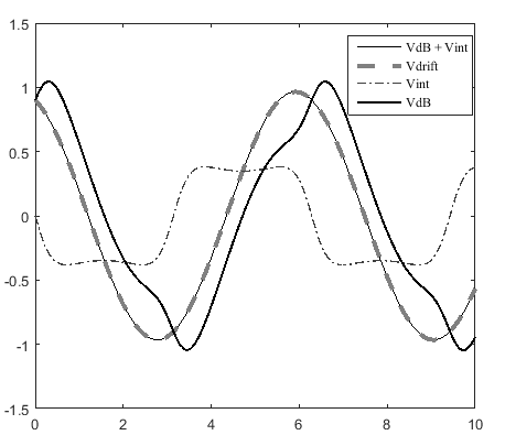
Figure 1: Plot of $v_{dBB},v_{int.},v_{dBB}+v_{int.}$ and $v_{drift}={d\over dt}(<x_{NL}>)$ with $<x_{NL}>=\int{d}^{3}x^{\prime}|\phi^{NL}(t,x^{\prime})|^{2}x^{\prime}/N_{NL}^{2}$) in function of time; space and time were rescaled and are of the order of unity.

To derive the plot 1, we imposed the following constraints:

$k^{self}/k^{ext.}=10^{3}$, $(<x_{NL}^{2}>-<x_{NL}>^{2})_{t=0}=\sqrt{\hbar\over\sqrt{(k^{ext}+k^{self})\cdot m}}$,

and $(<x_{NL}^{2}>-<x_{NL}>^{2})_{t=0}=10^{-3}(<x_{L}^{2}>-<x_{L}>^{2})_{t=0}$.

We observed that

(i) In the limit where $k^{self}/k^{ext.}$ is large enough, and provided at time $t=0$ the extent of the soliton $(<x_{NL}^{2}>-<x_{NL}>^{2})_{t=0}$ is comparable to the extent of the self-focused ground state ($\sqrt{\hbar\over\sqrt{k^{self}\cdot m}}$), and also quite smaller than the extent of the linear wave ($(<x_{NL}^{2}>-<x_{NL}>^{2})_{t=0}$ $<<$ ($<x_{L}^{2}>-<x_{L}>^{2})_{t=0}$), $\phi^{NL}(x,t)$ remains strongly peaked and oscillates around its central value throughout time.

(ii) In good approximation (the quality of the approximation being an increasing function of the ratio $k^{self}/k^{ext.}$), property 1 is confirmed by our numerical estimates. Indeed, as can be seen in figure 1, $v_{drift}$ is indistinguishable from $v_{dBB}+v_{int.}$.

(iii) In these conditions, property 2 is automatically satisfied.

(iv) We also noted that in good approximation (the quality of the approximation being an increasing function of the ratio $k^{self}/k^{ext.}$) the soliton $\phi^{NL}(x,t)$, as well as $\Psi^{NL}(x,t)$, follow classical trajectories.

3.2 Main conjecture.

The numerical results presented in the previous chapter (in particular observation (iv)) brought us to demonstrate the

Generalized Ehrenfest theorem.

To do so, let us consider the evolution equation

$${i}\hbar\frac{\partial\Psi(t,{{\bf x}})}{\partial t}=(-\hbar^{2}\frac{\Delta}{2m}+V^{L}(t,{{\bf x}})+V^{NL}(t,{{\bf x}}))\Psi(t,{{\bf x}}),$$ (22)

where $V^{NL}t,{{\bf x}})=-Gm^{2}\int{d}^{3}x^{\prime}|\Psi(t,{{\bf x}^{\prime}})|^{2}F(|{\bf x}-{\bf x^{\prime}}|)$, with $F$ a real function of $|{\bf x}-{\bf x^{\prime}}|$. Then the centre of its solution, denoted $<x>$ ($<x>=\int{d}^{3}x|\Psi(t,x)|^{2}x/N^{2}$ with $N^{2}=\int{d}^{3}x^{\prime}|\Psi(t,x^{\prime})|^{2}$) obeys the laws of classical dynamics in the limit where $<x^{2}>-<x>^{2}$ goes to zero.

To prove it, it suffices to note that $N$ remains constant throughout time, while

${d<x>\over dt}=<{i\hbar\over m}{\bf\nabla}>$, and

${d^{2}<x>\over dt^{2}}={1\over m}<[{\bf\nabla},V^{L}+V^{NL}]>={1\over m}<{\bf\nabla}V^{L}+{\bf\nabla}V^{NL}>.$

Now, $<{\bf\nabla}V^{NL}>$

$=\int{d}^{3}x^{\prime}|\Psi(t,x^{\prime})|^{2}\int{d}^{3}x|\Psi(t,x)|^{2}({\bf x}-{\bf x^{\prime}}){dF\over du}_{|u=|{\bf x}-{\bf x^{\prime}}|}=0,$ by symmetry so that

${d^{2}<x>\over dt^{2}}={1\over m}<{\bf\nabla}V^{L}>$.

In the limit where $<x^{2}>-<x>^{2}$ goes to zero, $<{\bf\nabla}V^{L}>\approx{\bf\nabla}V^{L}(<x>)$. Note that when $V^{L}$ is a quadratic function of the position (harmonic oscillator), $<{\bf\nabla}V^{L}>$ is always exactly equal to ${\bf\nabla}V^{L}(<x>).$

At this level, we face a serious problem: our original goal [23] was to derive dB-B dynamics from the non-linear dynamics (2) and the factorization ansatz (3). However, the trajectory of the soliton departs from dB-B dynamics, due to the presence of the residual contribution ${\bf v}_{int.}={\bf v}_{drift}-{\bf v}_{dB-B}$. Our simulations reveal that, in order to ensure the constraints imposed by Eherenfest’s theorem, ${\bf v}_{int.}$ “conspires” in order to be equal to ${\bf v}_{classical}-{\bf v}_{dB-B}$. This compensation is fragile however in the sense that ${\bf v}_{classical}-{\bf v}_{dB-B}$ contains the memory of the initial preparation process that eventually took place a long time ago. We shall conjecture here that in the practice some stochasticity is present that will wash out this memory and decorrelate ${\bf v}_{int.}$ from ${\bf v}_{classical}$. Averaging over this stochastic contribution we expect thus (and this is our main conjecture) that $<<{\bf v}_{int.}>>=0$ so that $<<{\bf v}_{drift}>>=<<{\bf v}_{dB-B}>>$, where the bracket $<<,>>$ represents an averaging over this extra-stochastic perturbation of the velocities that we conjecture to be present in nature.

Note that in the past Bohm, Vigier [10] and de Broglie [21] suspected the existence of a stochastic noise superposed to the quantum potential, necessary in their eyes in order to explain the irreversible in time convergence to quantum equilibrium. de Broglie wrote for instance in [21] (chapter XI: On the necessary introduction of a random element in the double solution theory. The hidden thermostat and the Brownian motion of the particle in its wave) the following sentences

…Finally, the particle’s motion is the combination of a regular motion defined by the guidance formula, with a random motion of Brownian character… any particle, even isolated, has to be imagined as in continuous “energetic contact” with a hidden medium, which constitutes a concealed thermostat. This hypothesis was brought forward some fifteen years ago by Bohm and Vigier [10], who named this invisible thermostat the “subquantum medium”….If a hidden sub-quantum medium is assumed, knowledge of its nature would seem desirable…

Our conjecture is a re-expression of the subquantum medium hypothesis invoked by Bohm and Vigier. At this level its deep nature is not clear yet: it could be the manifestation of a relativistic effect similar to the zitterbewegung (footnote 15 in appendix) or it could be of a fundamental nature [45]. It is out of the scope of the present paper to study these possibilities. It is worth noting however that in the case of bouncing oil droplets [24] such a stochastic disturbance of velocities is always present, due to the periodical forcing imposed to the bath. This explains why dB-B trajectories are never observed directly at the level of droplets but result from the averaging of a large number of trajectories [18, 19, 12].

4 Discussion and Conclusions.

Discussion: experimental validation.

The overwhelming majority of experiments [44, 51, 15, 7, 31] proposed so far in order to reveal the existence of intrinsic non-linearities at the quantum level (like e.g. the self-gravity interaction) is a priori doomed to fail, for what concerns our model, because their conceivers systematically took for granted that the wave function was normalised to unity. In the same line of thought, if our conjecture is correct, then trajectories of the self-collapsed solitons are very close to de Broglie-Bohm trajectories. Therefore we expect that our model cannot easily be falsified, to the same extent that the dB-B interpretation leads to the same predictions as the standard quantum theory (through the Born rule).

Even if our model is not relevant, and in the last resort its relevance ought to be confirmed or falsified by experiments, it could appear to be useful as a phenomenological tool.

For instance it was already applied by us [24] in the past to the phenomenology of bouncing oil droplets [18, 19, 12]. It is at this level that we expect that the validity of the approximations and hypotheses of our model could be confirmed or falsified.

The dynamics outlined here might also be relevant in the field of cold atoms physics [38] where effective non-linear self-focusing equations properly describe collective excitations of the atomic density [3]. As far as we know, no de Broglie like trajectory has yet been observed during such experiments.

In the same order of ideas, it would be highly interesting to investigate whether de Broglie like trajectories are good tools for describing optical and/or rogue waves [2, 37]. After all our factorisability ansatz could be applied to classical non-linear wave equations too.

Conclusions.

We have studied particular solutions of the S-N equation, in presence of an external potential, that behave as peaked solitons, due to the self focusing nature of self-gravitation. We showed that, if they exist and are stable, their shape is close in first approximation to the shape of the self-collapsed ground state, solution of (24) and, provided they remain peaked throughout time, they move in accordance with a generalized dB-B dynamics. These predictions were confirmed by numerical simulations. These simulations also showed that in the non-relativistic limit, the generalized dB-B dynamics is equivalent to classical dynamics, which is confirmed by a generalized Ehrenfest theorem. We conjecture however that if we add a stochastic field to the velocity field, dB-B dynamics will be restored. In last resort, this field could be a manifestation of the relativistic zitter bewegung (see appendix). In our approach, the linear wave function plays the role of an auxiliary computation tool (a pilot wave), and does not represent the particle which is represented by the soliton, which fits well into the double solution program of de Broglie.

We hope that the rather simple models treated in this paper will convince the reader that de Broglie’s ideas were maybe not that much surrealistic [27] and deprived of consistence. Our results indeed reinforces the dB-B picture according to which the particle non-locally and contextually explores its environment thanks to the nearly immaterial tentacles provided by the solution of the linear Schrödinger equation. This picture is not comfortable but it is maybe the price to pay to restore wave monism. Our conjecture (section 3.2) also reemphasises the necessity to invoke the existence of a subquantum medium in order to add to the regular and deterministic dB-B trajectories a random motion of brownian character. The brief incursion in the relativistic domain sketched in appendix suggests that the origin of this brownian motion could be linked to zitterbewegung [33, 41]. It would be highly interesting to try and reveal the existence of this subquantum medium experimentally, which is seemingly not an impossible task as suggested in ref.[50].

Last but not least, our analysis also confirms several prophetic intuitions originally presented by Louis de Broglie during the Solvay conference of 1927 [5].

5 Appendices.

5.1 The Schrödinger-Newton equation.

One can look for a “ground-state” solution to (1) in the form

$$\psi({\bf x},t)={e}^{-\frac{{i}E_{0}t}{\hbar}}\phi^{0}_{NL}({\bf x})~{}\!,$$ (23)

This leads to a stationary equation for $\phi^{0}_{NL}$

$$\frac{-\hbar^{2}}{2M}\Delta\phi^{0}_{NL}({\bf x})+GM^{2}\!\int\!d^{3}y~{}\!\frac{\big{|}\phi^{0}_{NL}({\bf y})\big{|}^{2}}{|{\bf x}-{\bf y}|}~{}\!\phi^{0}_{NL}({\bf x})=E_{0}\phi^{0}_{NL}({\bf x})~{}\!,$$ (24)

which was studied in astrophysics and is known under the name of the Choquard equation [39]. In [39], Lieb showed that the energy functional

$$E(\phi)=\frac{\hbar^{2}}{2M}\int\!{d}^{3}x~{}\big{|}\nabla\phi({\bf x})\big{|}^{2}-\frac{GM^{2}}{2}\iint\!{d}^{3}x{d}^{3}y~{}\!\frac{~{}\big{|}\phi({\bf y})\big{|}^{2}}{|{\bf x}-{\bf y}|}~{}\!\big{|}\phi({\bf x})\big{|}^{2}~{}\!,$$ (25)

is minimized by a unique solution $\phi^{0}_{NL}({\bf x})$ of the Choquard equation (24) for a given $L_{2}$ norm $N(\phi^{0}_{NL}({\bf x}))$. However no analytical expression is known for this ground state. Numerical treatments established that this ground state has a quasi-gaussian shape, and that its extent is, in the case $N(\phi^{0}_{NL}({\bf x}))=1$, of the order of ${\hbar^{2}\over GM^{3}}$. Then its energy is of the order of $G^{2}M^{5}/\hbar^{2}$. Otherwise, energy scales like $N(\phi^{0}_{NL}({\bf x}))^{3}$ [14]. Numerical evidence suggests the existence of a discrete spectrum of values for the energy (25) of the bound states solutions of (24). They can be written in the form $-\mathrm{e}_{n}\frac{G^{2}M^{5}}{\hbar^{2}}$, described in terms of dimensionless constants $\mathrm{e}_{n}$ as :

$$\mathrm{e}_{n}=\frac{a}{(n+b)^{c}}~{}\!,\quad n=0,1,2,\ldots~{}\!,$$ (26)

for approximated constants [6]

$$a=0.096\pm 0.01~{},\quad b=0.76\pm 0.01~{},\quad c=2.00\pm 0.01~{}\!.$$ (27)

The “ground state” for the Choquard equation corresponds, at $N=1$, to $n=0$ (see [14] and references therein for more details).

In summary, the S-N potential exhibits several interesting features that play an important role in our paper: it is self-focusing and possess a localized ground state of the type $\phi^{0}_{NL}({\bf x})e^{-iE_{0}t/\hbar}$ which behaves as a static bright soliton. The spectrum of negative energy eigenstates solutions of (24) is discrete. Moreover this potential scale like a Coulomb and/or Newtonian self-interaction in the sense that

$$V^{NL}(\lambda\Psi)=|\lambda|^{2}V^{NL}(\Psi)$$ (28)

5.2 Change of norm

Let us denote $H_{L}$ the linear part of the the full Hamiltonian in (8). It is not hermitian, so that $\sqrt{<\phi_{NL}|\phi_{NL}>}$, the L₂ norm of its solution $\phi_{NL}(t,{{\bf x}}))$ is not constant throughout time. The non-linear potentials considered by us preserve the L₂ norm however. We can thus evaluate the time derivative of $<\phi_{NL}|\phi_{NL}>$ by direct computation, either integrating by parts, or making use of the formula

$${d<\phi|O|\phi>\over dt}=$$

$$<\phi|{\partial O\over\partial t}|\phi>+{1\over i\hbar}<\phi|OH_{L}-H_{L}^{\dagger}O|\phi>$$

$$=<\phi|{\partial O\over\partial t}|\phi>+{1\over i\hbar}(<\phi|[O,Re.H_{L}]_{-}|\phi>$$ (29)

$$+{1\over\hbar}(<\phi|[O,Im.H_{L}]_{+}|\phi>),$$

where $O$ is an arbitrary observable, described by a self-adjoint operator, while $Re.H_{L}$ and $Im.H_{L}$, the real and imaginary parts of $H_{L}$ are self-adjoint operators defined through $2\cdot Re.H_{L}=H_{L}+H_{L}^{\dagger}$ and $2i\cdot Im.H_{L}=H_{L}-H_{L}^{\dagger}$. Here, the symbol $[,]_{-}$ ($[,]_{+}$) represents the (anti)commutator.

We find by direct computation that

$$Re.(-\frac{\hbar^{2}}{m}i{\bf\bigtriangledown}\varphi_{L}(t,{{\bf x}})\cdot{\bf\bigtriangledown})$$

$$=(-\frac{\hbar^{2}}{m}i{\bf\bigtriangledown}\varphi_{L}(t,{{\bf x}})\cdot{\bf\bigtriangledown})-(\frac{\hbar^{2}}{2m}i{\Delta}\varphi_{L}(t,{{\bf x}}))$$ (30)

and $Im.(-\frac{\hbar^{2}}{m}i{\bf\bigtriangledown}\varphi_{L}(t,{{\bf x}})\cdot{\bf\bigtriangledown})=(\frac{\hbar^{2}}{2m}{\Delta}\varphi_{L}(t,{{\bf x}}))$.

Therefore the guidance potential contributes to

${d<\phi_{NL}|\phi_{NL}>\over dt}={d<\phi_{NL}|1|\phi_{NL}>\over dt}$ by a quantity

$$<\phi_{NL}|(\frac{\hbar}{m}{\Delta}\varphi_{L}(t,{{\bf x}}))|\phi_{NL}>\approx(\frac{\hbar}{m}{\Delta}\varphi_{L}(t,{{\bf x}}))<\phi_{NL}|\phi_{NL}>),$$

due to the fact that, over the size of the soliton, $\varphi_{L}(t,{{\bf x}})$ and its derivatives are supposed to vary so slowly that we can consistently neglect their variation and put them in front of the L₂ integral.

The contribution of the $A_{L}-\phi_{NL}$ coupling to ${d<\phi_{NL}|\phi_{NL}>\over dt}$ is

$\frac{\hbar^{2}}{m}{1\over i\hbar}\int d^{3}{\bf x}(\frac{{\bf\bigtriangledown}A_{L}(t,{{\bf x}})}{A_{L}(t,{{\bf x}})}\cdot{\bf\bigtriangledown}(\phi_{NL}(t,{{\bf x}}))^{*}\phi_{NL}(t,{{\bf x}})-(\phi_{NL}(t,{{\bf x}}))^{*}\frac{{\bf\bigtriangledown}A_{L}(t,{{\bf x}})}{A_{L}(t,{{\bf x}})}\cdot{\bf\bigtriangledown}\phi_{NL}(t,{{\bf x}})).$

We now suppose that we are in right to neglect the variation of $\frac{{\bf\bigtriangledown}A_{L}(t,{{\bf x}})}{A_{L}(t,{{\bf x}})}$ in the integral above and we find, integrating by parts, a contribution $-2\frac{{\bf\bigtriangledown}A_{L}(t,{{\bf x_{0}}})}{A_{L}(t,{{\bf x_{0}}})}\cdot\int d^{3}{\bf x}(\phi_{NL}(t,{{\bf x}}))^{*}\frac{\hbar\bf\bigtriangledown}{mi}\cdot\phi_{NL}(t,{{\bf x}})$

Putting all these results together, we find that

$${d<\phi_{NL}|\phi_{NL}>\over dt}\approx\frac{\hbar}{m}{\Delta}\varphi_{L}(t,{{\bf x_{0}}})\cdot<\phi_{NL}|\phi_{NL}>$$

$$-2\frac{{\bf\bigtriangledown}A_{L}(t,{{\bf x_{0}}})}{A_{L}(t,{{\bf x_{0}}})}\cdot\int d^{3}{\bf x}(\phi_{NL}(t,{{\bf x}}))^{*}\frac{\hbar\bf\bigtriangledown}{mi}\cdot\phi_{NL}(t,{{\bf x}}).$$ (31)

5.3 The Dirac spinor.

In our view the S-N equation is a good candidate for fulfilling the de Broglie double solution program of 1927, in the same sense that Schrödinger’s equation was a good candidate for realizing de Broglie’s wave mechanics program of 1925. In the same line of thought, it is natural to look for a non-linear relativistic equation that would be to the S-N equations what are the Klein-Gordon or Dirac equations to the non-relativistic Schrödinger equation.

To do so let us consider the non-linear Dirac equation

$$\beta i\hbar\partial_{t}{\bf\Psi}(t,{\bf x})-\beta{\bf\alpha}c{\hbar\over i}{\bf\bigtriangledown}{\bf\Psi}(t,{\bf x})-(mc^{2}+V_{L}){\bf\Psi}(t,{\bf x})-V_{NL}{\bf\Psi}(t,{\bf x})=0.$$ (32)

where $\alpha$ and $\beta$ are the well-known Dirac matrices and

$$V_{NL}{\bf\Psi}(t,{\bf x})=-Gm^{2}\int{d}^{3}x^{\prime}(\frac{|\Psi(t,{{\bf x}^{\prime}})|_{4}^{2}}{|{{\bf x}-{\bf x}^{\prime}}|})\Psi(t,{{\bf x}}).$$ (33)

Here, $|\Psi(t,{{\bf x}^{\prime}})|_{4}^{2}$ represents the local Dirac density:

$|\Psi(t,{{\bf x}^{\prime}})|_{4}^{2}$=$({\bf\Psi}(t,{\bf x}))^{\dagger}\cdot_{4}{\bf\Psi}(t,{\bf x}))$, where the lower index ₄ refers to the spinorial in-product. Let us solve (32) imposing the ansatz

$${\bf\Psi}=\left(\begin{array}[]{c}\Psi_{0}(t,{{\bf x}})\\ \Psi_{1}(t,{{\bf x}})\\ \Psi_{2}(t,{{\bf x}})\\ \Psi_{3}(t,{{\bf x}})\\ \end{array}\right)=\left(\begin{array}[]{c}\Psi^{L}_{0}(t,{{\bf x}})\\ \Psi^{L}_{1}(t,{{\bf x}})\\ \Psi^{L}_{2}(t,{{\bf x}})\\ \Psi^{L}_{3}(t,{{\bf x}})\\ \end{array}\right)\phi_{NL}(t,{{\bf x}})={\bf\Psi_{L}}\phi_{NL}$$ (42)

where $\phi_{NL}(t,{{\bf x}})$ is a Lorentz scalar. We find

$$(\phi_{NL}(t,{{\bf x}}))(\beta i\hbar\partial_{t}{\bf\Psi^{L}}(t,{\bf x})-\beta{\bf\alpha}c{\hbar\over i}{\bf\bigtriangledown}{\bf\Psi^{L}}(t,{\bf x})-(mc^{2}+V_{L}){\bf\Psi^{L}}(t,{\bf x}))$$

$$+(\beta{\bf\Psi^{L}}(t,{\bf x}){i\hbar\partial\phi_{NL}(t,{{\bf x}})\over\partial t}-\beta{\bf\alpha}c{\bf\Psi^{L}}(t,{\bf x}){\hbar\over i}{\bf\bigtriangledown}\phi_{NL}(t,{{\bf x}})$$

$$+{\bf\Psi^{L}}(t,{\bf x})V_{NL}(|{\bf\Psi^{L}}\phi_{NL}|)\phi_{NL}(t,{{\bf x}}))=0,$$ (43)

that we solve in the same way as in the section 2 by requiring two constraints to be fulfilled:

$$\beta i\hbar\partial_{t}{\bf\Psi^{L}}(t,{\bf x})-\beta{\bf\alpha}c{\hbar\over i}{\bf\bigtriangledown}{\bf\Psi^{L}}(t,{\bf x})-(mc^{2}+V_{L}){\bf\Psi^{L}}(t,{\bf x})=0,$$ (44)

which is is the usual, linear, Dirac equation, and the non-linear constraint

$$\beta{\bf\Psi^{L}}(t,{\bf x}){i\hbar\partial\phi_{NL}(t,{{\bf x}})\over\partial t}-\beta{\bf\alpha}c{\bf\Psi^{L}}(t,{\bf x}){\hbar\over i}{\bf\bigtriangledown}\phi_{NL}(t,{{\bf x}})$$

$$+{\bf\Psi^{L}}(t,{\bf x})V_{NL}(|\Psi(t,{{\bf x}})|_{4})\phi_{NL}(t,{{\bf x}}))=0.$$ (45)

In agreement with (28), $V_{NL}$ supposedly scales like a Newtonian self interaction:

$$V_{NL}({\bf\Psi^{L}}\phi_{NL})=A_{L}^{2}V_{NL}(({\bf\Psi^{L}}(t,{\bf x})/A_{L})\cdot\phi_{NL}(t,{{\bf x}}))\phi_{NL}(t,{{\bf x}})$$ (46)

where

$$A_{L}=\sqrt{|\Psi^{L}_{0}(t,{{\bf x}})|^{2}+|\Psi^{L}_{1}(t,{{\bf x}})|^{2}+|\Psi^{L}_{2}(t,{{\bf x}})|^{2}+|\Psi^{L}_{3}(t,{{\bf x}})|^{2}}.$$ (47)

At this level, a serious problem appears: equation (45) consists of four equations. In the non-relativistic limit [41] and in absence of external magnetic field, spin decouples and can be factorized, but in general the four equations implicitly contained in equation (45) are NOT equivalent to each other.

A posteriori, we feel free to formally tackle the problem by proceeding as follows. We firstly decompose ${\bf\Psi}$ into its projection along ${\bf\Psi_{L}}$ and its projection along the 4-spinors orthogonal to ${\bf\Psi_{L}}$:

$${\bf\Psi}={\bf\Psi_{L}}({\bf\Psi_{L}}^{\dagger}{\bf\Psi})+(1-{\bf\Psi_{L}}\cdot{\bf\Psi_{L}}^{\dagger}){\bf\Psi}$$ (48)

Let us introduce $\phi_{NL}(t,{{\bf x}})$ through ${\bf\Psi_{L}}({\bf\Psi_{L}}^{\dagger}{\bf\Psi})$ = ${\bf\Psi_{L}}\phi_{NL}(t,{{\bf x}})$, as well as the auxillary spinor ${\bf\delta\Psi}$=$(1-{\bf\Psi_{L}}\cdot{\bf\Psi_{L}}^{\dagger}){\bf\Psi}$, which allows us to rewrite (48) as follows:

$${\bf\Psi}={\bf\Psi_{L}}\phi_{NL}+{\bf\delta\Psi}$$ (49)

In a second time, let us simply neglect ${\bf\delta\Psi}$, in a grossly coarse-grained approach, in order to gain more insight about the physics of the problem, but keeping in mind however that there is a serious difficulty hidden under the rug at this level.

Retrospectively, our approximation justifies the ansatz (42). 4-multiplying (45) by $({\bf\Psi^{L}}(t,{\bf x}))^{\dagger}\beta$ and dividing by $({\bf\Psi^{L}}(t,{\bf x}))^{\dagger}\cdot_{4}{\bf\Psi^{L}}(t,{\bf x}))=A_{L}^{2}$ we get

$${i\hbar\partial\phi_{NL}(t,{{\bf x}})\over\partial t}={\bf v^{L}_{Dirac}}(t,{{\bf x}}){\hbar\over i}{\bf\bigtriangledown}\phi_{NL}(t,{{\bf x}})$$ (50)

$$+<\beta>_{4}\cdot A_{L}^{2}\cdot V_{NL}(\phi_{NL})\phi_{NL}(t,{{\bf x}}).$$

where $<\beta>_{4}$=$({\bf\Psi^{L}}(t,{\bf x}))^{\dagger}\beta{\bf\Psi^{L}}(t,{\bf x}))$/$({\bf\Psi^{L}}(t,{\bf x}))^{\dagger}\cdot_{4}{\bf\Psi^{L}}(t,{\bf x}))$ while ${\bf v^{L}_{Dirac}}$ obeys

$${\bf v^{L}_{Dirac}}\equiv{({\bf\Psi^{L}})^{\dagger}\alpha c{\bf\Psi^{L}}\over({\bf\Psi^{L}})^{\dagger}{\bf\Psi^{L}}}$$ (51)

As is well-known, the conservation equation associated to the linear Dirac equation is ${\partial A^{2}_{L}\over\partial t}=-div(A_{L}^{2}\cdot{\bf v_{Dirac}}(t,{{\bf x_{0}}}))$. The dB-B guidance equation is thus nothing else than (51) [46, 34]. Now, if we suppress in (8) the kinetic energy and the factor proportional to $A_{L}$, we find an equation which is formally equivalent to (50). Therefore, by repeating computations similar to those made in section 2, one can easily show that the dB-B guidance equation linked to Dirac’s equation (51) is exactly satisfied. Furthermore, resorting to the conservation equation ${\partial A^{2}_{L}\over\partial t}=-div(A_{L}^{2}\cdot{\bf v_{Dirac}}(t,{{\bf x_{0}}}))$, it is straightforward to establish the validity of property 2 as in the non-relativistic case studied before. For instance ${{dA_{L}\over dt}\over A_{L}}={-1\over 2}{1\over<\phi_{NL}|\phi_{NL}>}{d<\phi_{NL}|\phi_{NL}>\over dt}$

Consequently, we are entitled to look for peaked wave functions of the form

$${\bf\Psi}=\left(\begin{array}[]{c}\Psi_{0}(t,{{\bf x}})\\ \Psi_{1}(t,{{\bf x}})\\ \Psi_{2}(t,{{\bf x}})\\ \Psi_{3}(t,{{\bf x}})\\ \end{array}\right)={1\over A_{L}}\cdot\left(\begin{array}[]{c}\Psi^{L}_{0}(t,{{\bf x}})\\ \Psi^{L}_{1}(t,{{\bf x}})\\ \Psi^{L}_{2}(t,{{\bf x}})\\ \Psi^{L}_{3}(t,{{\bf x}})\\ \end{array}\right)\cdot\phi^{\prime}_{NL}(t,{{\bf x}}),$$ (60)

for which we know that

(Property 1) the barycentre of $\phi^{\prime}_{NL}$ moves along the hydrodynamical flow lines of Dirac’s linear equation, at velocity ${\bf v_{Dirac}}$.

(Property 2) the L₂ norm of $\phi^{\prime}_{NL}(t,{{\bf x}})$ is constant throughout time.

As in the non-relativistic case, the amplitude $A_{L}$ is an auxiliary function that disappears at the end of the computation of ${\bf\Psi}$. It is worth noting that we did not demonstrate the existence of a ground state of the type $\phi^{0}_{NL}$ in the relativistic case. We also suspect that the self-gravitational potential $V_{NL}$ proposed in (33) is not the right candidate in a relativistic context because it is obviously not Lorentz covariant. In any case, it is beyond the scope of our paper to characterize in detail what “really” happens at the level of the soliton. We expect for instance [24] that in the case of an electron, the size of the soliton is of the order of 10^-57 meter, well beyond the Planck scale. Our main aim in the present section was merely to suggest that hopefully properties 1 and 2 exhibit some structural invariance when we pass from the non-relativistic to the relativistic regime.

References

- [1] E. Abraham, S. Colin and A.Valentini. Long-time relaxation in pilot-wave theory J. Phys. A: Math. Theor. 47, 395306, 2014.
- [2] N. Akhmediev, A. Ankiewicz, and M. Taki. Waves that appear from nowhere and disappear without a trace. Physics Letters A, 373:675-678, 2009.
- [3] C. Anastopoulos and B-L Hu. Problems with the Newton-Schrödinger equations. New J.Phys. 16 085007, 2014.
- [4] E. Ruiz Arriola and J. Soler. A Variational Approach to the Schrödinger-Poisson System: Asymptotic Behaviour, Breathers, and Stability. J. Stat. Phys., 103(5-6):1069–1105, 2001.
- [5] G. Bacciagaluppi and A. Valentini. Quantum Theory at the Crossroads: Reconsidering the 1927 Solvay Conference. Cambridge University Press (2010), and quant-ph/0609184.
- [6] D.H. Bernstein, E. Giladi, and K.R.W. Jones. Eigenstates of the gravitational Schrödinger equation. Mod. Phys. Lett. A, 13(29):2327–2336, 1998.
- [7] I. Bialynicki-Birulal. On the linearity of the Schrödinger equation. Brazilian Journal of Physics, 35(2A): 211-215 (2005).
- [8] D. Bohm. A Suggested Interpretation of the Quantum Theory in Terms of “Hidden” Variables. I. Phys. Rev., 85(2):166–179, 1952.
- [9] D. Bohm. A Suggested Interpretation of the Quantum Theory in Terms of “Hidden” Variables. II. Phys. Rev., 85(2):180–193, 1952.
- [10] D. Bohm and J.P. Vigier. Model of the Causal Interpretation of Quantum Theory in Terms of a Fluid with Irregular Fluctuations Phys. Rev., 96, 208, 1954.
- [11] F. Brezzi and P.A. Markowich. The Three–Dimensional Wigner-Poisson Problem: Existence, Uniqueness and Approximation. Mathematical Methods in the Applied Sciences, 14(1):35–61, 1991.
- [12] J.W.M. Bush. Pilot-Wave Hydrodynamics. Ann. Rev. Fluid Mech., 49:269-292.
- [13] S. Colin. Relaxation to quantum equilibrium for Dirac fermions in the de Broglie-Bohm pilotwave theory. Proc. R. Soc. A., 468 (2140):1116-1135, 2012.
- [14] S. Colin, T. Durt, and R. Willox. Can quantum systems succumb to their own (gravitational) attraction? Class. Quantum Grav., 31:245003, 2014.
- [15] S. Colin, T. Durt, and R. Willox. Crucial tests of macrorealist and semi-classical gravity models with freely falling mesoscopic nanospheres. preprint (2014) arXiv:1402.5653v3.
- [16] S. Colin and W. Struyve. Quantum non-equilibrium and relaxation to equilibrium for a class of de Broglie-Bohm-type theories. New J. Phys. 12, 043008 (2010).
- [17] G. Contopoulos, N. Delis and C. Efthymiopoulos. Order in de Broglie - Bohm quantum mechanics J. Phys. A: Math. Theor. 45, 16530, 2012.
- [18] Y. Couder and E. Fort. Single-Particle Diffraction and Interference at a Macroscopic Scale. Phys. Rev. Lett., 97:15410, 2006.
- [19] Y. Couder, A. Boudaoud, S. Protière and E. Fort. Walking droplets, a form of wave-particle duality at macroscopic scale? Europhysics News Vol. 41, No. 1, 14-18 2010.
- [20] L. de Broglie. Une tentative d’interprétation causale et non linéaire de la mécanique ondulatoire: la théorie de la double solution. Paris: Gauthier- Villars, (1956). English translation: Nonlinear wave mechanics: A causal interpretation. Elsevier, Amsterdam 1960.
- [21] L. de Broglie. Interpretation of quantum mechanics by the double solution theory Annales de la Fondation Louis de Broglie, 12, 4, 1987, english translation from a paper originally published in the book Foundations of Quantum Mechanics- Rendiconti della Scuola Internazionale di Fisica Enrico Fermi, IL Corso, B. d’ Espagnat ed. Academic Press N.Y.1972.
- [22] L. Diósi. Gravitation and quantum-mechanical localization of macro-objects. Phys. Lett. A, 105:199–202, 1984.
- [23] T. Durt Generalized guidance equation for peaked quantum solitons: the single particle case. Arxiv quant-ph 160203133 v1 2016.
- [24] T. Durt Generalized guidance equation for peaked quantum solitons and effective gravity. Euro. Phys. Lett., 114, n∘ 1, 2016.
- [25] T. Durt et al. de Broglie-Bohm dynamics and butterfly effect in a Stern-Gerlach measurement. In preparation.
- [26] C. Efthymiopoulos, C. Kalapotharakos, and G. Contopoulos. Origin of chaos near critical points of quantum flow. Phys. Rev. E, 79(3):036203, 2009.
- [27] B-G Englert, M. Scully, G. Süssman, H. Walther. Surrealistic Bohm Trajectories Zeit. für Nat. A, 47, 12, 1992.
- [28] D. Fargue. Permanence of the corpuscular appearance and non linearity of the wave equation. In S. Diner et al., editor, The wave-particle dualism, pages 149–172. Reidel, 1984.
- [29] J. Fronteau; R. Jacquier. Vers un modèle non-hamiltonien de l’oscillateur harmonique, Annales de l’I.H.P. Physique théorique, 16, 2: 119–132, 1972.
- [30] G. Gouesbet. Hidden Worlds in Quantum Physics. (Dover Books on Physics, 2013)
- [31] A. Grossardt, J. Bateman, H. Ulbricht, and A. Bassi. Optomechanical test of the Schr’́odinger-Newton equation. Phys. Rev. D, 93:096003, 2016.
- [32] A. Grossardt, Approximations for the free evolution of self-gravitating quantum particles Phys. Rev. A, 94: 022101, 2016.
- [33] D. Hestenes. The Zitterbewegung Interpretation of Quantum Mechanics Founds. of Phys., 20, 10, 1990.
- [34] P.R. Holland. The Quantum Theory of Motion (Cambridge University Press, 1993)
- [35] R. Illner and P.F. Zweifel. Global Existence, Uniqueness and Asymptotic Behaviour of Solutions of the Wigner-Poisson and Schrödinger-Poisson Systems. Mathematical Methods in the Applied Sciences, 17:349–376, 1994.
- [36] K. R. W. Jones. Newtonian Quantum Gravity. Aust. J. Phys., 48:1055–1081, 1995.
- [37] P. Koonath, D. R. Solli, C. Ropers, and B. Jalali. Optical rogue waves. Nature Letter, 450(19):1054-1057, 2007.
- [38] G. Labeyrie, E. Tesio, P. M. Gomes, G.-L. Oppo, W. J. Firth, G. R. M. Robb, A. S. Arnold, R. Kaiser, and T. Ackemann Optomechanical self-structuring in cold atomic gases Nature Photon. 8, 321 2014.
- [39] E.H. Lieb. Existence and Uniqueness of the Minimizing Solution of Choquard’s Nonlinear Equation. Studies in Applied Mathematics, 57:93–105, 1977.
- [40] C.E. Lopez-Fortin, M. Hatifi and T. Durt, work in progress.
- [41] A. Messiah. Quantum Mechanics Vol. 2 North Holland Publishing Company, 1967.
- [42] R. Penrose. On Gravity’s Role in Quantum State Reduction. General Relativity and Gravitation, 28(5):581–600, 1996.
- [43] H. Poincaré. La fin de la matière Athenaeum 4086, 201-202, 1906, Sur la dynamique de l’ électron Rendiconti del Circolo matematico di Palermo 21, 129-176, 1906.
- [44] L. Smolin. Quantum fluctuations and inertia. Physics Letters A, 113:408, (1986).
- [45] S. Sonego. Interpretations of the Hydrodynamical formalism of quantum mechanics. Founds. Phys., 21(10):1135–1181, (1991).
- [46] T. Takabayasi Relativistic hydrodynamics of the Dirac matter. Suppl. Prog. Theor. Phys. 4, 1-80 1957.
- [47] A. Valentini and H. Westman. Dynamical origin of quantum probabilities. Proc. R. Soc. A, 461:253-272, 2005.
- [48] J. R. van Meter. Schrödinger-Newton “collapse” of the wave-function. Class. Quant. Grav., 28:215013, 2011.
- [49] J.-P. Vigier. Particular solutions of a non-linear Schrödinger equation carrying particle-like singularities represent possible models of de Broglie’s double solution theory. Phys. Lett. A, 135(2): 99: 105, 1989.
- [50] White, H., March, P., Lawrence, J., Vera, J., Sylvester, A., Brady, D., and Bailey, P., Measurement of Impulsive Thrust from a Closed Radio-Frequency Cavity in Vacuum, Journal of Propulsion and Power, 1-12, 2016. ISO 690
- [51] H. Yang, H. Miao, D-S. Lee, B. Helou, and Y. Chen. Macroscopic quantum mechanics in a classical spacetime. Phys. Rev. Lett., 110:170401, 2003.