Holistic Influence Maximization: Combining Scalability and Efficiency with Opinion-Aware Models

Abstract

The steady growth of graph data from social networks has resulted in wide-spread research in finding solutions to the influence maximization problem. In this paper, we propose a holistic solution to the influence maximization (IM) problem. (1) We introduce an opinion-cum-interaction (OI) model that closely mirrors the real-world scenarios. Under the OI model, we introduce a novel problem of Maximizing the Effective Opinion (MEO) of influenced users. We prove that the MEO problem is NP-hard and cannot be approximated within a constant ratio unless P=NP. (2) We propose a heuristic algorithm OSIM to efficiently solve the MEO problem. To better explain the OSIM heuristic, we first introduce EaSyIM – the opinion-oblivious version of OSIM, a scalable algorithm capable of running within practical compute times on commodity hardware. In addition to serving as a fundamental building block for OSIM, EaSyIM is capable of addressing the scalability aspect – memory consumption and running time, of the IM problem as well.

Empirically, our algorithms are capable of maintaining the deviation in the spread always within 5% of the best known methods in the literature. In addition, our experiments show that both OSIM and EaSyIM are effective, efficient, scalable and significantly enhance the ability to analyze real datasets.

1 Motivation

Growth and pervasiveness of online social networks is no longer a new phenomenon. They have become an integral part of the day-to-day life of almost every Internet user. Their wide-spread reach paves the way for a host of applications – (1) Viral marketing/ad-targeting [24, 44, 9], (2) Outbreak detection [25, 35], (3) Community formation, evolution and detection [10, 12, 40], (4) Recommendations using social-media [49, 14] and many more. The influence maximization (IM) problem [32] with its applicability in solving the above mentioned problems and beyond, has thus, been one of the most widely studied problems over the past decade. This problem is to identify a set of seed nodes so that the overall spread of information in a network, which is the potential collective impact of imparting that piece of information to these nodes, is maximized.

Given that the objective of IM is to maximize the spread of information about a content, which can be a product, person, event and many more, an important aspect of this problem is the underlying information diffusion model. A diffusion model defines the dynamics of information propagation and also controls the way this information is perceived by the nodes in a network. Nevertheless, a substantially large fraction of the literature in this field has focussed on devising efficient and scalable algorithms [32, 35, 28, 13, 46, 23, 18, 17, 31, 29, 19, 33, 42, 22, 21] for IM using the classical information diffusion models [32, 44]. The two fundamental diffusion models proposed by Kempe et al. [32] – Independent Cascade (IC) and Linear Threshold (LT) have been almost exclusively followed in majority while extended in a small fraction of all the subsequent work.

Figure 1: A sample representation of the Twitter network.

Having said that, the most obvious limitation of these models is that the notion of spread, of a set of seed-nodes $S$, is defined as a function of the number of nodes that get activated using these seeds. The problem with this definition is two fold – (1) Each node is considered to be contributing fully and positively towards the spread of information about a content without considering the personal opinion of the nodes which could be even negative, (2) A newly active node is always considered to perceive the information with the same intent as that of the node that activated it, while the former may tend to disagree with the latter owing to the interactions between them in the past. These scenarios are not scarce in real-world settings, where a node can possess an opinion (Def. 4) towards a content which is the subject of IM. Moreover, usually past interactions (Def. 5) between a pair of nodes govern the way in which any new information originating from one of the two would be perceived by the other and vice-versa. To better understand these aspects, let us consider a (sample) real-world scenario in Example 1.

Example 1

Suppose Apple wants to market, utilizing the notion of viral-marketing, the iPhone 6 Plus using the Twitter network given a marketing budget of $1$ seed-node. Figure 1 portrays a snapshot of such a network consisting of $4$ nodes. Nodes $A$ and $C$ follow $B$, while $D$ follows $A$ and $C$. The opinion ($o$) of a node towards the new iPhone can be calculated using its opinion towards similar products in the past – previous iPhone models or phones belonging to the same market segment. For example, the node $A$ has $o_{A}=0.8$, which means that she held highly positive opinions towards previous iPhone models or similar products. The opinion for other nodes can be computed in a similar way. Moreover, each edge possesses an additional parameter, called the interaction ($\varphi$) probability. In our example, the directed edge $BC$ has $\varphi_{BC}=0.8$ which means that the node $C$ perceives the information originating from the node $B$ with the same intent $4$ out of $5$ times. In other words, $C$ agrees with $B$ $4$ out of $5$ times while disagrees otherwise.

In the light of above discussions, it is intuitive that despite of being widely adopted, the fundamental (opinion-oblivious) diffusion models lack the power to leverage the expressibility of the social networks of today, namely – Facebook, Twitter etc. Thus, there is a need to explore potential extensions, over and above these models, with the ability to better model information diffusion under real-world scenarios. To further this cause, we incorporate the concepts of opinion and interaction [27, 43, 38] from the social media domain and propose a new Opinion-cum-Interaction (OI) model of information diffusion capable of addressing the limitations discussed above. Using the OI model, we define a more realistic notion of opinion-spread (Defs. 6 and 7).

Let us try to analyze the importance of opinion-spread using the example in Figure 1. As discussed earlier, opinion-oblivious diffusion models, viz. IC, rely on the influence probability ($p$) alone without paying heed to the personal opinion of the activated nodes, which may even be negative. Thus, the likelihood of $C$ being chosen as a seed under the IC model is fairly high, owing to the high value of $p_{CD}$ which in turn results in high (opinion-oblivious) spread. However, owing to $o_{D}$ being negative it will always decrease the overall opinion-spread if activated. Thus, $C$ might not be the best choice for a seed-node. Moreover, a model capable of capturing the effect of opinions, viz. OI, will penalize $C$ and thus decrease its likelihood of being chosen as a seed node.

We strengthen the above mentioned observation further, by plotting the opinion-spread against the number of seeds for different real datasets (details in Sec. 4). Figure 2 shows that the opinion-spread obtained by the seeds selected using the OI model is much better when compared to that using the IC model, and thus, establishes the importance of OI over the IC/LT models of information-diffusion with better conformance to the real-world scenarios.

As mentioned above, there has not been much research in devising opinion-aware information-diffusion models, with IC-N [16] and OC [48] being the only two models capable of incorporating negative opinion in the diffusion process. Despite of their capability to model opinions, they possess the following limitations.

(1) Constrained and Specific: The IC-N model is rather simplistic, where a negatively activated node retains its opinion throughout its lifetime, while a quality-factor qf (same for each node) defines the probability of transitioning to a negative opinion for the positively activated nodes. Although, a uniform qf allows retention of submodularity, which further facilitates extension of existing algorithms for IM to this setting, it renders the model too specific.

(2) Simplistic diffusion dynamics: The IC-N model possesses a strict constraint that a negatively activated node will always activate other nodes as negative. This assumption ignores the personal opinion of a node completely, and will be violated when the target node possesses a highly positive opinion about a content.

The OC model, where the change in opinion of a node is dependent upon its own opinion and the opinion of the nodes that activate it, does not possess the above two limitations. The OC model thus, facilitates a more involved process of modelling opinions at an added cost of losing submodularity.

(3) Lack capability to capture Interaction: Both IC-N and OC lack the capability to capture the way in which information is perceived between a pair of nodes (interaction) in the network.

(4) Lack of backward-compatibility with fundamental diffusion models: The IC-N model is tuned to work with IC at the first layer, while the OC model is designed to work with LT alone.

The OI model attempts to address these limitations by allowing – (1) Nodes to possess different opinions, (2) Edges to possess an interaction probability for modelling the perception of information between a node-pair, and (3) Capability of working with both IC and LT at the first layer. In addition to the analytical explanations, Figure 2 also shows that the opinion-spread with seeds selected using OI is better when compared to those selected using OC. In summary, the OI model is a more generic, natural and realistic model when compared to IC-N and OC.

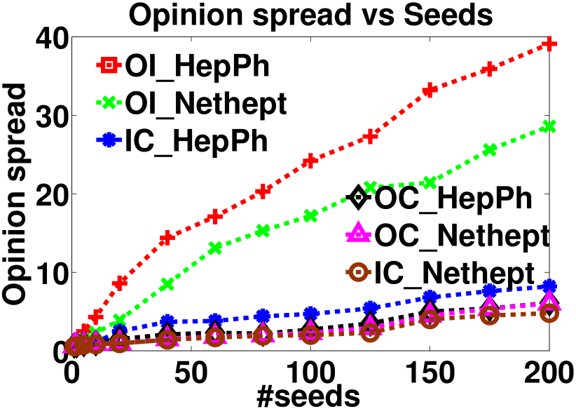
Figure 2: Opinion spread for different diffusion models.

Having successfully motivated (both qualitatively and empirically) and differentiated (from current state-of-the-art) the OI model, we propose a novel problem (MEO) of maximizing the spread of information under opinion-aware settings. Since MEO is NP-hard and difficult to approximate within a constant ratio, we incorporate ideas from the opinion-oblivious scenarios to design scalable algorithms for the opinion-aware case. We propose OSIM, capable of maximizing the opinion-spread while accommodating for the change of opinion as the information propagates. To this end, we first analyze a representative set of algorithms for IM under the fundamental diffusion models.

Although, the Kempe’s GREEDY algorithm [32] provides the best possible approximation guarantees for the IM problem, it is inefficient. The CELF++ [28] algorithm with optimizations over GREEDY renders it as the most efficient technique within this class of algorithms. However, these techniques never improved the asymptotic time-complexity of IM and thus, cannot be employed for large graphs. To further this, recent works employed the use of sampling with memoization [13, 46, 23, 45], with TIM⁺ and its improvement IMM being the most efficient, to achieve superior efficiency while retaining approximation guarantees. However, these algorithms cannot be termed scalable owing to their exorbitantly high memory footprint. For example, the memory footprint of TIM⁺ can be as high as 100 GB for a graph with $1M$ nodes and $3M$ edges which is not uncommmon these days. Owing to these limitations, neither CELF++ nor TIM⁺ serve as potential candidates for extensions to opinion-aware scenarios. Our proposition, EaSyIM, tackles these problems by incorporating the idea that influence of a node can be estimated using a function of the number of simple paths starting at that node. Note that paths of length $l$ from a node $u$ can be calculated as the sum of all paths of length $l-1$ from its neighbors. We exploit this idea to devise data-structures and algorithms capable of running in linear space and time. This renders our algorithm scalable yet efficient. Therefore, EaSyIM is chosen for extensions to the opinion-aware case to produce OSIM, which being fundamentally similar possesses the same analysis as EaSyIM.

Contributions. In summary, we make the following contributions. We propose a holistic solution to the IM problem. Towards that,

• We introduce the OI model (Sec. 2.2) which, to the best of our knowledge, is the most generic information diffusion model with the ability to address most of the limitations in the existing models and closely mirror real-world scenarios. In addition to this, we are the first to motivate the need of opinion-aware models by citing a novel application – analyzing churn, using real-world data (Sec. 4.1.2).

• Under OI, we propose a novel problem of maximizing the effective opinion of influenced users, called MEO (Sec. 2.3).

• We propose effective, efficient and scalable algorithms (Sec. 3), namely – OSIM and EaSyIM, that run in linear time $O(k\mathcal{D}(m+n))$ and space $O(n)$.

• We provide thorough theoretical analyses (Sec. 3.4) to prove the effectiveness of our algorithms. We believe that such an in-depth analysis for the algorithms that estimate influence as a function of simple paths is not present in the literature.

• Through an in-depth empirical analysis (Sec. 4), we show that our algorithms are the first to possess the capability of handling huge graphs on commodity-hardware and provide the best trade-off between running-time and memory-consumption, while retaining the quality of spread.

The rest of the paper is organized as follows. In Section 2, we introduce a generic opinion-aware information diffusion model and present the problem statement. Section 3 describes our algorithm and its analysis. In Section 4, experimental results are presented. Section 5 highlights the related work before Section 6 concludes.

2 Opinion Aware IM

In this section, we first introduce the basic concepts of the IM problem and build upon them to describe the Opinion-cum-Interaction (OI) model for information diffusion in detail. The notations used in the rest of the paper are summarized in Table 1.

2.1 Preliminaries

The objective of the IM problem is to capture the dynamics of information diffusion for maximizing the spread of information in a network. To this end, we first define the notions of seed and active nodes in the context of fundamental (opinion-oblivious) information diffusion models, namely – IC and LT. Next, we use these concepts to define the notion of spread of information in a network.

Definition 1 (Seed Node)

A node $v\in V$ that acts as the source of information diffusion in the graph $G(V,E)$ is called a seed node. The set of seed nodes is denoted by $S$.

Definition 2 (Active Node)

A node $v\in V$ is deemed active if either (1) It is a seed node ($v\in S$) or (2) It receives information, under the dynamics of information diffusion models, from a previously active node $u\in V_{(a)}$. Once activated, the node $v$ is added to the set of active nodes $V_{(a)}$.

Given a seed node $s\in S$ and a graph $G(V,E)$, an information diffusion model $\mathcal{I}$ defines a step-by-step process for information propagation. Having defined the notions of seed and active nodes, we now introduce the dynamics of the IC and LT models. For both the IC and LT models, the first step requires a seed node $s\in S$ to be activated and added to the set of active nodes $V_{(a)}$. Under the IC model, at any step $i$ each newly activated node $u\in V_{(a)}$ gets one independent attempt to activate each of its outgoing neighbours $v\in\textbf{Out}(u)$ with a probability $p_{(u,v)}$. However, under the LT model, a node $v$ gets activated if the sum of weights $w_{(u,v)}$ of all the incoming edges $(u,v)$ originating from active nodes $\forall u\in\textbf{In}(v)_{(a)}$ exceeds the activation threshold $\theta_{v}$ of v, i.e., $\sum_{u\in\textbf{In}(v)_{(a)}}w(u,v)\geq\theta_{v}$. Once a node becomes active, it remains active in all the subsequent steps. This diffusion process runs for each seed-node $s\in S$ until no more activations are possible. Eventually, the cardinality of the set of active nodes $|V_{(a)}|$, barring the number of seeds $k=|S|$, constitute the spread of a given set of seed nodes. Formally,

Definition 3 (Spread)

Given an information diffusion model $\mathcal{I}$ (opinion-oblivious), the spread $\Gamma(S)$ of a set of seed nodes $S$ is defined as the number of nodes, barring the nodes in $S$, that get activated using these seed nodes. Mathematically, $\Gamma(S)=|V_{(a)}|-|S|$.

Item	Definition
$V$	Set of vertices; $|V|=n$.
$E$	Edge set for the nodes in $V$; $|E|=m$.
$\mathcal{D}$	Diameter of the graph.
$S$	Set of seed nodes.
$k=|S|$	Number of seed nodes.
$\textbf{Out}(u)$	Set of outgoing neighbours of $u$.
$\textbf{In}(v)$	Set of incoming neighbours of $v$.
$p_{(u,v)}$	Influence probability of $u$ on $v$ for IC.
$\theta_{v}$	Activation threshold of $v$; $\theta_{v}\in[0,1]$.
$o_{v}$	Personal opinion of $v$; $o_{v}\in[-1,1]$.
$w_{(u,v)}$	Weight on the edge $u\rightarrow v$ for LT; $w_{(u,v)}\in[0,1]$.
$\varphi_{(u,v)}$	Interaction probability from $u$ to $v$.
$\Gamma(S)$	Spread obtained by set of seed nodes ($S$).
$\sigma(S)$	Expected value of spread by seeds in $S$; $\mathbb{E}(\Gamma(S))$.
$V_{(a)}$	The set of active nodes; $V_{(a)}\subseteq V$.
$\lambda$	Penalty parameter on negative opinion spread.
$l$	Maximum path length for score-assignment, $1\leq l\leq\mathcal{D}$.
$\mathcal{L}(u\leadsto v)$	Length of a given $u\leadsto v$ path.
$\gamma_{v}(u)$	Contribution of $v$ to $\sigma(u)$, using approximate scores (Sec. 3.2).
$\gamma^{*}_{v}(u)$	Contribution of $v$ to $\sigma(u)$, using GREEDY[32].
$\mathbb{P}_{uv}$	The set of all $u$-$v$ paths; $\{u\leadsto v\}$
$t_{(u,v)}$	#$u$-$v$ paths – #paths starting at $u$ and ending at $v$.
$s^{d}_{(u,v)}$	Contribution of $v$, via a $d$-length $u$-$v$ path, to $\sigma(u)$.
$\Delta^{l}(u)$	Score assigned to $u$, using all $u\leadsto v$ paths of length $\leq l$.

Table 1: Summary of the notations used.

Given the above defined concepts, the IM problem aims at identifying a set of seed nodes capable of maximizing the expected spread of information in a network under a fixed budget on the number of seed nodes. More formally, Given a graph $G=(V,E)$, a fundamental (opinion-oblivious) information diffusion model $\mathcal{I}$ (IC/LT) with specifics defined as above and a budget $k$, find a set of seed nodes, $S\subseteq V\mid k=|S|$, that maximizes the expected value of information spread $\sigma(S)=\mathbb{E}[\Gamma(S)]$ in this graph.

2.2 Opinion-cum-Interaction (OI) Model

The OI model for information diffusion serves as an extension over the IC and LT models to facilitate opinion-aware IM. The fundamental models are modified to include a second layer attributed to modelling the diffusion and change of opinion(Def. 4) in the network. As opposed to the IC/LT models, where a newly activated node (oblivious to its opinion) is always considered to be contributing positively towards the information spread (Def. 3), the OI model considers the spread (opinion-spread, Defs. 6 and 7) of information under an opinion-aware scenario – where the contribution of a newly activated node could as well be negative.

The OI model can be easily tuned, with minor modifications, to work with both IC and the LT models. The specifics of OI, thus, change depending on the underlying fundamental information diffusion model. Before moving to the model specifics, it is useful to introduce the notions of opinion ($o$) of a node and interaction ($\varphi$) between two nodes. Usually, the objective of IM is to maximize the spread of information about a specific content viz. product, topic, person, event etc. Having said that, the opinion of a node is always defined in the context of a particular content to denote the personal preference of this node towards that content. Formally,

Definition 4 (Opinion)

The opinion of a node $v\in V$ consists of two sub-components – (1) an orientation $(${negative, neutral, positive}$)$ towards a content and (2) strength $([0,1])$ that quantifies its preference towards that content. The opinion of a node is, thus, denoted as $o_{v}\in[-1,1]$.

As opposed to opinion which is associated with properties of a node alone, interaction aims at capturing the effect of the dyadic relationship between any two nodes to better model the process of information diffusion. Formally,

Definition 5 (Interaction)

The interaction probability (directed) between two nodes $u,v\in V$, denoted as $\varphi_{(u,v)}\in[0,1]$, is defined as a fraction of the times an information content shared by $u$ gets accepted by $v$ with the same orientation as that of $u$.

For example, if two nodes $u$ and $v$ agree with each other $1$ out of $5$ times in the past, then $\varphi_{(u,v)}=\varphi_{(v,u)}=1/5=0.2$. As discussed in Sec. 1, the opinion of a node towards a new content can be estimated from the previously held opinions by this node towards similar contents in the past. As opposed to this, the interaction probabilities (directed, $\varphi_{(u,v)}$ might not be equal to $\varphi_{(v,u)}$) between two nodes is rather generic and can be estimated by accounting for all possible interactions between these nodes in the past. Next, we describe the specifics of the OI model.

We model the underlying network as a directed graph $G=(V,E)$ with parameters $p,w,\theta,o,\varphi$, where $|V|=n$ and $|E|=m$ denote the set of vertices and edges respectively. The parameters have similar meanings as discussed earlier in this section. Oblivious to the underlying information diffusion model (IC or LT), each node $v\in V$ possesses an opinion towards a new content denoted by $o_{v}\in[-1,1]$. Specifically the sign of $o_{v}$ indicates the orientation and the value denotes the strength. More formally, $o_{v}>0$, $o_{v}=0$, and $o_{v}<0$ indicate positive, neutral and negative orientation respectively. In addition, $o_{v}=-1$ denotes a strong negative opinion while $o_{v}=+1$ denotes a strong positive opinion. Moreover, each edge $(u,v)\in E$ possess $\varphi_{(u,v)}\in[0,1]$, that refers to the probability of a node $v$ acquiring the same opinion as that of $u$, considering only the contribution from node $u$. $\varphi_{(u,v)}=0$ indicates that $v$ never agrees with $u$, while $\varphi_{(v,u)}=0.5$ indicates that $u$ agrees with $v$ half of the time. The dynamics of the model are as follows.

Under the IC model, the first step involves activation of each seed node $s$, in the selected seed set $S$ ($|S|$ = $k$), with its opinion $o_{s},\forall s\in S$, while all other nodes remain inactive. At any step $i$, if a node $u$ (which was activated at step $i-1$) activates another node $v$ then the final opinion ($o_{v}^{\prime}$) of $v$ is dependent upon both, its initial opinion $o_{v}$ and the final opinion ($o_{u}^{\prime}$) of the node $u$. More formally, each node $u$, contributes $o_{u}^{\prime}$ with a probability $\varphi_{(u,v)}$ and $-o_{u}^{\prime}$ with a probability $1-\varphi_{(u,v)}$. The final opinion of the node $v$ is $o^{\prime}_{v}=\frac{o_{v}+(-1)^{\alpha}o_{u}^{\prime}}{2}$, where $\alpha=0$ with a probability of $\varphi_{(u,v)}$ and $\alpha=1$ with a probability of $1-\varphi_{(u,v)}$.

Under the LT model, the first step witnesses the same set of initializations as done for OI under the IC model. At any step $i$, if a node $v$ gets activated (by the set of nodes $\textbf{In}(v)_{(a)}$, activated at previous steps) then the final opinion $o_{v}^{\prime}$ of $v$ is dependent upon both, its initial opinion $o_{v}$ and the final opinion $o_{u}^{\prime}$ for all the nodes $u\in\textbf{In}(v)_{(a)}$. The contributions made by each node to the opinion of the node $v$ is the same as discussed above for OI under the IC model. The final opinion of the node $v$ is $o^{\prime}_{v}=(o_{v}+\frac{1}{|\textbf{In}(v)_{(a)}|}\sum\limits_{u\in\textbf{In}(v)_{(a)}}(-1)^{\alpha_{(u,v)}}o_{u}^{\prime})/2$, where $\alpha_{(u,v)}=0$ with a probability of $\varphi_{(u,v)}$ and $\alpha_{(u,v)}=1$ with a probability of $1-\varphi_{(u,v)}$.

Once a node becomes active, it remains active with the same effective opinion in all the subsequent steps. The information propagation process runs until no more activations are possible. With these extensions, we aim to solve the IM problem under settings that closely mirror real-world scenarios. Before moving ahead, we revisit Example 1 and analyze the difference between spread and opinion-spread with stating the importance of the latter in real-world scenarios using Example 2.

Example 2

Let us consider the construction described in Example 1 with all the model-specific parameters present in Figure 1. For the sake of brevity, the analysis of spread in this scenario assumes (1) the IC model and (2) the OI model using IC at the first-layer. The influence probability ($p$, of an edge) possesses the same meaning as for the fundamental models. Since $p_{AD}=0.8$, the expected spread of $A$ under the IC model $(\sigma(A))$ is $0.8$. Similarly for other nodes: $\sigma(B)=0.3628,\ \sigma(C)=0.9$ and $\sigma(D)=0$. Thus, $C$ is selected as the seed node. Since $D$ agrees with $A$ with a probability of $\varphi_{AD}$ and disagrees otherwise, the expected opinion-spread of $A$ under the OI model is expressed as $\sigma^{o}(A)=p_{AD}\big{(}\varphi_{AD}(o_{D}+o_{A})/2+(1-\varphi_{AD})(o_{D}-o_{A})/2\big{)}=0.8\big{(}0.9(-0.3+0.8)/2+0.1(-0.3-0.8)/2\big{)}=0.136$. Similarly for other nodes: $\sigma^{o}(B)=-0.022564,\ \sigma^{o}(C)=-0.351$ and $\sigma^{o}(D)=0$. Thus, $A$ is selected as the seed node. An interesting observation is that, the seed identified using the IC model, i.e. $C$, would have resulted in the worst-possible opinion-spread. This clearly shows the importance of the notion of opinion-spread under the OI model, over opinion-oblivious spread using the IC model, in real-world scenarios where opinion of nodes and interaction between nodes play an important part in governing the process of information propagation.

Next, we formally state the MEO problem followed by its tractability analysis.

2.3 Problem Formulation

Using the concepts described in the previous sections, we formally define the notion of spread under the opinion-aware (OI) model, called Opinion Spread. While, under the opinion oblivious models spread can simply be stated as the total number of nodes that get activated with a given set of seed nodes, a more involved notion of spread is required under the opinion-aware settings.

Definition 6 (Opinion spread)

Opinion spread of a seed set $S$, denoted by $\Gamma^{o}(S)$, is defined as the sum of final opinions of the nodes in the activated set $V_{(a)}\setminus S$, when $S$ is the chosen seed set, i.e., $\Gamma^{o}(S)=\sum\limits_{v\in V_{(a)}\setminus S}o_{v}^{\prime}$.

Definition 7 (Effective opinion spread)

Effective opinion spread of a seed set $S$, denoted by $\Gamma^{o}_{\lambda}(S)$, is defined as the weighted difference between the opinion spread of nodes with positive orientation and the opinion spread of nodes with negative orientation, i.e., $\Gamma^{o}_{\lambda}(S)=\big{(}\sum\limits_{o_{v}^{\prime}>0}o_{v}^{\prime}-\lambda\sum\limits_{o_{v}^{\prime}<0}|o_{v}^{\prime}|\big{)};\forall v\in V_{(a)}\setminus S$, in the set of activated nodes $V_{(a)}\setminus S$, where $\lambda$ is the penalty on negative opinion spread.

We call the problem of maximizing the effective opinion spread under the OI model as Maximizing the Effective Opinion of the Influenced Users (MEO) problem, which is defined formally as follows.

Problem 1

Given a graph $G=(V,E)$, the opinion-aware (OI) model with specifics defined as in Sec. 2.2 and a budget $k$, find a set of seed nodes, $S\subseteq V\mid k=|S|$, that maximizes the expected value of the effective opinion spread $\sigma^{o}_{\lambda}(S)=\mathbb{E}[\Gamma^{o}_{\lambda}(S)]$.

2.4 Properties of MEO under the OI model

2.4.1 NP-hardness

Lemma 1

The MEO problem is NP-hard.

Proof 2.1.

The IM problem is reducible to an instance of the MEO problem under the OI model, when $o_{v}=1$, $\forall v\in V$ and $\varphi_{(u,v)}=1,$ $\forall(u,v)\in E$. It is known that any generalization of a NP-hard problem is also NP-hard. Since, the IM problem is NP-hard [32], the MEO problem is NP-hard as well.

2.4.2 Submodularity

A function $f(\cdot)$ is submodular if the marginal gain from adding an element to a set $S$ is at least as high as the marginal gain from adding it to a superset of $S$. Mathematically,

$$f(S\cup\{x\})-f(S)\geq f(T\cup\{x\})-f(T)$$

for all elements $x$ and all pairs of sets $(S,T)$, where $S\subseteq T$. For submodular and monotone functions, the greedy algorithm of iteratively adding the element with the maximum marginal gain approximates the optimal solution within a factor of ($1-1/e$) [41].

Lemma 2.2.

The opinion spread as a function $\Gamma(\cdot)$ in a graph $G$, is neither monotone nor submodular.

Proof 2.3.

Let us consider a bipartite graph $G(V,E)$ (Figure 3a) containing two sets of nodes $X$ and $Y=V\setminus X$. The set $X$ contains $n_{x}=|X|$ nodes while the set $Y$ contains $n_{y}=|Y|,n_{y}\geq 2n_{x}$ nodes. Moreover, let us assume that the opinions of the nodes $\forall x_{i}\in X$ to be $o_{x_{i}}=+1$, while that of nodes $\forall y_{j}\in Y$ to be $o_{y_{j}}=0$. There exist directed edges from each node $x_{i}\in X$ to two consecutive nodes $y_{2i-1},y_{2i}\in Y$. Further, the influence probabilities are initialized as $p_{(u,v)}=1,\forall(u,v)\in E$ and the interaction probabilities $\varphi$ associated with all but the last two edges is $1$, which attain a value of $0$. Mathematically, $\varphi_{x_{i},y_{j}}=1\mid 1\leq i\leq n_{x}-1,j=2i-1$ or $j=2i$ while $\varphi_{x_{i},y_{j}}=0\mid i=n_{x},j=2i-1$ or $j=2i$. An analysis of the properties of the spread function $\Gamma(\cdot)$, assuming the above construction, is presented next.

Consider a scenario where the set of seeds $S$ is initialized with a single node $x_{i}\mid 1\leq i\leq n_{x}-1$. With this seed, both of the nodes $y_{2i-1}$ and $y_{2i}$ will get activated with final opinion $+1/2$. Hence, the effective spread $\Gamma^{o}(S)=2\times(1/2)=+1$. Now if the node $x_{|X|}$ is added to the set $S$, the nodes $y_{2|X|-1}$ and $y_{2|X|}$ will also get activated. The final opinion of these newly activated nodes will be $-1/2$ each. The effective spread of the updated seed set is $\Gamma^{o}(S)=1-1=0$. On adding another node $x_{j}\mid j\neq i$ and $1\leq j\leq n_{x}-1$ to the set $S$, the nodes $y_{2j-1}$ and $y_{2j}$ will become active with a final opinion of $1/2$ each. Thus, the effective spread is now $\Gamma^{o}(S)=0+1=1$. In the above case it can be seen that the effective spread varied from $1\rightarrow 0\rightarrow 1$ on subsequent additions of nodes to the seed set. This clearly shows that the opinion spread function $\Gamma^{o}(S)$ is neither monotone nor submodular.

(a) Submodularity

(b) Tractability

Figure 3: Reductions for the submodularity and tractability analysis of MEO.

Using Lemma 2.2, it is evident that a greedy algorithm cannot produce a $1-1/e$ approximate solution to the MEO problem. Next, we further prove that $\nexists$ any algorithm capable of approximating MEO within a constant ratio.

Theorem 2.4.

Approximating MEO within a constant ratio is not possible unless $P=NP$.

Proof 2.5.

We show that the classical set cover problem can be decided in polynomial time if an approximation, with a constant ratio, for MEO exists in polynomial time. To this end, we reduce the set cover problem to an instance of MEO. Given a set of elements $Q=\{q_{1},\ldots,q_{n}\}$ and a collection of subsets $R=\{R_{1},\ldots,R_{m}\}$ where $R_{i}\subseteq Q,\forall i\in\{1,\ldots,m\}$, the set-cover decision problem returns true if $\exists C\subseteq R;|C|=k$ and $\cup C_{j}=Q,\ \forall C_{j}\in C$.

Now given the set-cover problem, we construct a graph as shown in Figure 3b to obtain an instance of MEO by adding three layers of nodes in addition to a sink node. For each subset $R_{i}\in R$, a node $x_{i}$ is added in the first layer of the graph with opinion $o_{x_{i}}=0$. In the second layer, for each element $q_{i}\in Q$, we add a node $y_{i}$ with opinion $o_{y_{i}}=\frac{1}{n}$. We add a third layer containing $m+n-2$ nodes denoted by $z_{i}$ with opinion $o_{z_{i}}=-\frac{1}{2n}$. Along with this, we add a sink node $s$ with opinion $o_{s}=-1+\frac{1}{n}$. Now, a directed edge $(x_{i},y_{j})$ is added iff $q_{i}\in R_{j}$. For each node $y_{i}$ in the second layer, edges $(y_{i},z_{j}),\forall j\in\{1,2,\ldots,m+n-2\}$ are added in the graph. To finalize this construction, we add the edge $(z_{i},s),\forall i\in\{1,2,\ldots,m+n-2\}$ .

For the IC model, all the edges $(u,v)\in E$ are assigned $p_{(u,v)}=1$ and $\varphi_{(u,v)}=1$. Moreover, the LT model uses the same activation threshold for each node $\theta_{u}=1$. It can be seen that for both these models, the seeds should be chosen from the first layer (any of the $x_{i}$’s), because they will activate $y_{j}$’s which in turn will activate any of the $z_{i}$’s and thus, $s$ would always be activated.

We instantiate MEO with $\lambda=1$. Without loss of generality, assuming $\exists$ a set-cover of size $k$, $C=\{x_{1},x_{2},\ldots,x_{k}\}$, then choosing these nodes as seeds ensures the maximum spread. The final opinion of $y_{i}$, $o_{y_{i}}^{\prime}=(0+\frac{1}{n})/2=\frac{1}{2n}$. Similarly, the final opinion of $z_{i}$, $o_{z_{i}}^{\prime}=\frac{1}{2n}-\frac{1}{2n}=0$ and the final opinion of $s$, $o_{s}^{\prime}=(0-1+\frac{1}{n})/2=-\frac{1}{2}+\frac{1}{2n}$. Hence, the spread = $n\frac{1}{2n}+0-\frac{1}{2}+\frac{1}{2n}=\frac{1}{2n}>0$. When a set cover of size $k$ does not exist, the maximum spread achieved is $|Q^{\prime}|\frac{1}{2n}+0-\frac{1}{2}+\frac{1}{2n}\leq(n-1)\frac{1}{2n}-\frac{1}{2}+\frac{1}{2n}=0$, where $Q^{\prime},|Q^{\prime}|\leq n-1$ is the maximum number of elements covered by the $k$ chosen sets. Hence, the maximum spread achieved when the set-cover does not exist is $0$.

If there is a polynomial time algorithm which approximates MEO within a constant ratio, then we can decide the set-cover problem in polynomial time using the above mentioned reduction. In other words, if an approximate algorithm gives a spread $\leq 0$ on the reduced graph, then a set-cover does not exist while a set-cover exists if the spread $>0$. This renders the set-cover problem decidable in polynomial time, which means P=NP. Therefore, approximating MEO within a constant ratio is NP-hard.

3 Algorithm

3.1 Outline of our Algorithm

To solve the MEO problem efficiently, we propose a technique as outlined in Algorithm 1. We first assign a score (line $4$), to each node $u\in V$ of the graph $G(V,E)$, by aggregating the contributions of all paths starting at $u$. We prove that if the score assignment is correct (we will specify exactly what is meant by “correct” later), then the expected value of the influence spread achieved using our algorithm is the same as that achieved using the GREEDY gold standard [32]. The correctness of our score assignment algorithms, both for the opinion-oblivious (EaSyIM) and the opinion-aware (OSIM) case, holds perfectly for trees. Moreover, in a conclusive discussion, we show that the error introduced in case of graphs is small as well. Through detailed analyses and experiments we show that our results do not deviate much from that of the GREEDY algorithm.

On completion of the score assignment step, the node possessing the maximum score is selected as the seed node (lines $5$–$9$). In order to ensure the sets of nodes activated by each selected seed node to be disjoint; the last step of the seed-selection algorithm (line 11) keeps track of all the previously activated nodes as a set ($V_{(a)}$). This enables the score assignment step to discount the contributions of all the previously activated nodes in subsequent iterations. The above process continues until $k$ seeds are selected.

Next, we describe the score-assignment algorithms – (1) EaSyIM and its extension (2) OSIM in detail. The algorithms are fundamentally similar for both, opinion-oblivious and opinion-aware, cases.

3.2 Score Assignment

The score assignment step, similar to ASIM [26], leverages the idea that the probability of a node $v$ to get activated by a seed node $u$ is dependent upon the number of simple paths from $u$ to $v$ in $G$. Thus, a simple function of the number of paths from a node $u$ to all other nodes $v\in V\setminus\{u\}$ can be used to assign a score to $u$. This score-assignment is further used to rank all the nodes $v\in V$ in an order determining their expected spread $\sigma(v)$. To this end, the scores assigned to a node $u$ ($\Delta^{l}(u)$), is computed by aggregating the contributions of all $u\leadsto v$ paths of length at most $l$ ($\mathcal{L}(u\leadsto v)\leq l$). We start with a description of the score assignment step for the opinion-oblivious (EaSyIM) case and then follow it up with the opinion-aware (OSIM) case. The following explanations of the score assignment algorithms assume the IC model of information diffusion. Their extensions to the linear threshold (LT) and the weighted cascade (WC) models are discussed in Sec. 3.3.

3.2.1 EaSyIM

As mentioned in Sec. 3.2, a function of the number of directed simple paths from a node $u$ to another node $v$ can be used to estimate the influence of the former on the latter. However, direct application of this notion to design solutions for the influence maximization problem poses two inherent challenges of maintaining – 1) Scalability and Efficiency, 2) Correctness guarantees. Since, counting the number of $s$-$t$ paths is shown to be in $\#P$-Complete [47], computing the expected influence of a node is $\#P$-hard for both the IC [17] and the LT [19] models. This further shows that it is impossible to come up with a score-assignment algorithm capable of correctly selecting a seed-node with maximum influence.

Algorithm 1 ScoreGREEDY

0:  Graph $G=(V,E)$,#seeds $k=|S|$, $l$

0:  Seed set $S$

1:  $S,V_{(a)}\leftarrow\emptyset$

2:  for i = 1 to k do

3:     $max,\ maxId\leftarrow 0$

4:     $\Delta^{l}\leftarrow AssignScore(G(V\setminus V_{(a)},E),o,p,\varphi,l)$

5:     for each $u\in V$ do

6:        if $\Delta^{l}(u)>max$ then

7:           $max\leftarrow\Delta^{l}(u),\ maxId\leftarrow u$

8:        end if

9:     end for

10:     $S\leftarrow S\cup\{maxId\}$

11:     Update $V_{(a)}$ with nodes activated by the newly selected seed-node ($maxId$)

12:  end for

Algorithm 2 AssignScore

0:  Graph $G=(V,E)$, $o$, $p$, $\varphi$, $l$

0:  $\Delta^{l}$

1:  if ${{\neg}}\ Opinion$ then

2:     $\Delta^{l}\leftarrow EaSyIM(G(V,E),p,l)$ //Opinion-Oblivious

3:  else

4:     $\Delta^{l}\leftarrow OSIM(G(V,E),o,p,\varphi,l)$ //Opinion-Aware

5:  end if

Although counting $s$-$t$ paths is $\#P$-Complete, there exists a polynomial time algorithm to count all possible walks of length at most $l$ between all node-pairs ($\forall(u,v)\in V$) in $G$ that takes $O(n^{3}\log l)$ time and consumes $O(n^{2})$ memory. The $Path$-$Union$ ($PU$) algorithm (Algorithm 3) extends this algorithm by initializing the adjacency matrix of the graph $M$ with the pair-wise influence probabilities (line $2$). Since the contributions of these paths cannot be simply aggregated, we define a new operator $\otimes$ for matrix multiplication (line $4$). Under this operator, the multiplication of $i^{th}$ row ($M[i][:]$) with $j^{th}$ column ($M[:][j]$) is defined using Eq. 1. This algorithm has an inherent problem that it counts cyclic paths as well, which eventually serves as a source of error while computing the influence of a node. We try to reduce the impact of this error for each node, by removing the contributions of the walks that pass through the node itself (lines $5$–$7$). Finally, the score of each node $u$ is computed as indicated in line $10$.

$$M[i][j] =M[i][:]\otimes M[:][j]=\bigcup_{k=1}^{n}M[i][k]\times M[k][j].$$ (1)

Owing to its huge time and space complexity, the $PU$ algorithm cannot be used in practice. The EaSyIM algorithm (Algorithm 4) describes a score-assignment method, with efforts to tackle this scalability bottleneck. Paths of length $l$ from a node $u$ can be calculated as the sum of all paths of length $l-1$ from its neighbors. $\Delta^{l}(u)\ (\forall u\in V)$ is defined as the weighted sum of the number of paths of length at most $l$ starting from $u$ and is computed as indicated in line $5$ of Algorithm 4. The weight for each path is defined as the product of probabilities $p_{(u,v)}$ of the edges composing that path. EaSyIM score of a node $u$ tries to mimic closely the expected value of the spread when $u$ is chosen as a seed node.

For every iteration of EaSyIM, the outgoing neighbours $\textbf{Out}(u)$ of each node $u\in V$ are visited to accumulate the contribution of paths of different lengths ($l$). The parameter $l$ can be as large as the diameter ($\mathcal{D}$) of the graph. Thus, the total time taken by the score-assignment step using the EaSyIM algorithm is $O(\mathcal{D}(m+n))$, in the worst-case. Moreover, the total time taken for selecting $k$ seeds using our modified greedy algorithm (ScoreGREEDY) is $O(k\mathcal{D}(m+n))$. The space complexity of this algorithm is $O(n)$, as the only additional overhead is the storage of a score ($O(1)$) at each node. A detailed analysis on the correctness of $PU$ and EaSyIM algorithms is present in Sec. 3.4.1.

Algorithm 3 $Path$-$Union(PU)$

0:  Graph $G=(V,E)$, $n=|V|$, $p$, $l$

0:  $\Delta^{l}$

1:  Matrix $M^{n\times n}\leftarrow 0$, $PU\leftarrow I^{n\times n}$

2:  $\Delta^{0}(u)\leftarrow 0$ ($\forall u\in V$), $M[u][v]\leftarrow p_{(u,v)}$ ($\forall u,v\in V$)

3:  for each $i\in\{1,\ldots,l\}$ do

4:     $PU\leftarrow PU\otimes M$

5:     for each $v\in V$ do

6:        $PU[v][v]\leftarrow 0$

7:     end for

8:     for each $u\in V$ do

9:        for each $v\in V$ do

10:           $\Delta^{i}(u)\leftarrow\Delta^{i-1}(u)+PU[u][v]$

11:        end for

12:     end for

13:  end for

14:  return $\Delta^{l}$

3.2.2 OSIM

We now describe the OSIM algorithm (Algorithm 5), to assign a score to each node of a graph for the opinion-aware case. This algorithm extends EaSyIM by accommodating for the change in opinion (Sec. 2.2) during the information propagation process. Since, the change in opinion is captured using a second layer over and above the activation step of a node, we incorporate the use of the following intermediate terms $\alpha_{i}$, $or_{i}$ and $sc_{i}$ for each node. At each iteration, these intermediate terms contain only the contributions for a given path length $i\leq l$. For a given node $u$, the term $or_{i}(u)$ contains the weighted sum of the initial opinions of all nodes, reachable via paths of length $i$ starting at $u$ (line $6$). In other words, $or_{i}(u)$ constitutes the contribution of nodes reachable by $u$ via paths of length $i$ to its score ($\Delta^{i}(u)$), without considering the change in opinion during information propagation. Similarly, the term $\alpha_{i}(u)$ computes the weighted sum of the interaction probabilities ($\varphi$) associated with all the paths of length $i$, starting at $u$ (line $7$). For a given path of length $i$ ($\mathcal{L}(u\leadsto v)=i$), $sc^{v}_{i}(u)$ contains the contributions of all nodes in this path to the change in opinion of node $v$ (line $8$). The term $sc_{i}(u)$ further contains the aggregation of $sc_{i}^{v}(u)$ for all $i$ length paths starting at $u$ (line $10$).

Algorithm 4 EaSyIM

0:  Graph $G=(V,E)$, $p$, $l$

0:  $\Delta^{l}$

1:  $\Delta^{i}(v)\leftarrow 0$ ($\forall i\leq l,\ \forall v\in V$)

2:  for each $i\in\{1,\ldots,l\}$ do

3:     for each $u\in V$ do

4:        for each $v\in\textbf{Out}(u)$ do

5:           $\Delta^{i}(u)\leftarrow\Delta^{i}(u)+p_{(u,v)}(1+\Delta^{i-1}(v))$

6:        end for

7:     end for

8:  end for

9:  return $\Delta^{l}$

Similar to EaSyIM, the weight for each path is defined as the product of probabilities $p_{(u,v)}$ of the edges composing that path. Moreover, the weight, for term $\alpha_{i}$, additionally incorporates the interaction probabilities ($\varphi_{(u,v)}$) as well. In line $11$, the score for a node $u$ ($\Delta^{i}(u)$) is iteratively updated with the aggregation of all the intermediate terms ($or_{i}(u),\alpha_{i}(u),$ and $sc_{i}(u)$). Finally, $\Delta^{l}(u)$ contains the score of a node $u$ with the contributions of all paths of length at most $l$, starting at $u$. Note that, since the loop invariants in lines $2,3$ and $5$ of OSIM is exactly the same as that of EaSyIM (lines $2,3$ and $4$), its time and space complexity analysis is exactly the same as EaSyIM.

3.3 Extensions

The extension to the WC model is rather trivial, as instead of assuming a fixed value of $p$ (usually $p=0.1$ for IC), we assign $\forall(u,v)\in E,p_{(u,v)}=1/|\textbf{In}(v)|$. All the previously presented algorithms can readily accommodate this change. However, the changes required for the LT model are much more involved.

Extension to the LT model is difficult when considering its classical definition where each node possesses a threshold, while it is quite intuitive using the live-edge model. Kempe et al. proved the equivalence between the LT and the live-edge model in [32]. Similar to the IC and WC models, under the live-edge model each edge $(u,v)\in E$ possesses a probability with which $u$ activates its neigbour $v$. Moreover given an instance of the graph, it has an additional constraint of each node possessing one (live) incoming edge. The expected value of spread is then calculated using the spreads achieved for each of these graph instances. Thus, by associating influence probabilites with each edge and generating various graph instances satisfying the above constraint, our algorithms get extended to the live-edge model and hence, the LT model without undergoing any change. Since each node can possess only a single incoming edge, the error introduced in score-assignment owing to the non-disjoint nature of the paths gets completely removed (a unique $u$–$v$ path $\forall u,v\in V$), which in turn facilitates stronger theoretical analysis for the LT model when compared to the IC and WC models.

Algorithm 5 OSIM

0:  Graph $G=(V,E)$, $o$, $p$, $\varphi$, $l$

0:  $\Delta^{l}$

1:  $\alpha_{0}(u)\leftarrow 1$, $or_{0}(u)\leftarrow o_{u}$, $sc_{0}(u),\Delta^{0}(u)\leftarrow 0$ ($\forall u\in V$)

2:  for each $i\in\{1,\ldots,l\}$ do

3:     for each $u\in V$ do

4:        $\alpha_{i}(v),or_{i}(v),\ sc_{i}(v)\leftarrow 0$

5:        for each $v\in\textbf{Out}(u)$ do

6:           $or_{i}(u)\leftarrow or_{i}(u)+p_{(u,v)}or_{i-1}(v)$

7:           $\alpha_{i}(u)\leftarrow\alpha_{i}(u)+p_{(u,v)}\alpha_{i-1}(v)(2\varphi_{(u,v)}-1)/2$

8:           $sc_{i}(u)\leftarrow sc_{i}(u)+p_{(u,v)}sc_{i-1}(v)$

9:        end for

10:        $sc_{i}(u)\leftarrow sc_{i}(u)+o_{u}\alpha_{i}(u)$

11:        $\Delta^{i}(u)\leftarrow\Delta^{i-1}(u)+\frac{or_{i}(u)+sc_{i}(u)+o_{u}\alpha_{i}(u)}{2}$

12:     end for

13:  end for

14:  return $\Delta^{l}$

Next, we present a detailed analysis for the EaSyIM and the OSIM algorithms for score-assignment, assuming the IC model of information diffusion. Sec. 3.4.2 provides discussions on methods to extend these analyses to the WC and LT models as well.

3.4 Analysis of Score Assignment

As a first step towards analyzing our algorithms, we derive a relation between the expected value of spread achieved using a set of seed-nodes and any possible partition of this set.

Lemma 3.6.

$\sigma(A\cup B)=\sigma(A)+\sigma_{\sigma(A)}(B)$

Proof 3.7.

Using Kempe’s  [32] analysis of the IC model it can be seen that,

$$\sigma( A\cup B)=\sum_{X}P(X)\sigma_{X}(A\cup B)$$

$$=\sum_{X}P(X)\big{(}\sigma_{X}(A)+\sigma_{X}(B)-\sigma_{X}(A\cap B)\big{)}$$

$$=\sum_{X}P(X)\sigma_{X}(A)+\sum_{X}P(X)\big{(}\sigma_{X}(B)-\sigma_{X}(A\cap B)\big{)}$$

$$=\sigma(A)+\sigma_{\sigma(A)}(B).$$ (2)

A similar analysis can be done for the LT model using the reduction to the live-edge model [32]. Under the live-edge model each node possesses a single (live) incoming edge, thus, a node $v$ is activated via a path either from a node in $A$ or in $B$.

$$\sigma(A\cup B) =\sum_{X}P(X)\sigma_{X}(A\cup B)$$

$$=\sum_{X}P(X)\big{(}\sigma_{X}(A)+\sigma_{X}(B)\big{)}$$

$$=\sum_{X}P(X)\sigma_{X}(A)+\sum_{X}P(X)\sigma_{X}(B)$$

Since, $\sigma(A)$ and $\sigma(B)$ are disjoint,

$$\sigma(A\cup B) =\sigma(A)+\sigma_{\sigma(A)}(B).$$ (3)

The next result uses Lemma 3.6 to prove that the ScoreGREEDY algorithm produces a $1-1/e$ approximate solution to the IM problem, under the condition that the score assigned to each node captures the expected value of spread using that node.

Lemma 3.8.

Given a graph $G(V,E)$, if score-assignment is correct, i.e., the score assigned to each node $\Delta^{l}(u)$ captures the expected value of its spread $\Delta^{l}(u)=\sigma_{\sigma(S)}(\{u\})$ where $S$ is the set of seed nodes, then $\sigma(S_{k})=\sigma(S_{k}^{*})$ where $S_{k}$ is the set of seed nodes selected using the ScoreGREEDY algorithm while $S_{k}^{*}$ is the set selected using GREEDY algorithm.

Proof 3.9.

If $k=1$, $\sigma(S_{k})=\sigma(S_{k}^{*})$ because ScoreGREEDY$(G,k,l)$ chooses the node with the maximum score. Since the score assigned to each node captures the expected value of its spread, the seed-node selected by the former is the same as that selected by the GREEDY algorithm. Let us assume that $\sigma(S_{k})=\sigma(S_{k}^{*})$ holds for $k=i$. Now for $k=i+1$,

$$\sigma(S_{i+1}^{*}) =\sigma(S_{i+1}^{*})-\sigma(S_{i}^{*})+\sigma(S_{i}^{*})$$

Paritioning $S_{i+1}$ as $S_{i}\cup\{u_{i+1}\}$, Lemma 3.6 yields the following,

$$=\sigma_{\sigma(S^{*}_{i})}(\{u_{i+1}\})+\sigma(S_{i}^{*})$$

$$=\sigma_{\sigma(S_{i})}(\{u_{i+1}\})+\sigma(S_{i})$$

$$=\Delta^{l}(\{u_{i+1}\})+\sigma(S_{i})$$

$$=\sigma(S_{i+1}).$$

Since $\sigma(S_{i+1})=\sigma(S_{i+1}^{*})$, by the principle of mathematical induction $\sigma(S_{k})=\sigma(S_{k}^{*})$ holds $\forall k$.

Conclusion 1

Given a correct score assignment algorithm, the ScoreGREEDY algorithm produces a $1-1/e$ approximate solution to the IM problem.

As discussed in Sec. 3.2, it is impossible to devise a correct scoring algorithm, i.e., a score-assignment that captures the expected value of spread for each node, for graphs. Thus, the ScoreGREEDY algorithm cannot produce a $1-1/e$ approximate solution to the IM problem. Next, we show a detailed analysis of both EaSyIM and OSIM score assignment strategies.

3.4.1 EaSyIM

In this section, we first state the causes for the introduction of errors in $PU$ & EaSyIM, and follow it up by a concrete analysis on the exact quantification of these errors.

We first show the amount of error introduced by $PU$ for DAGs. Although, the $PU$ algorithm can enumerate the exact number of paths for DAGs, errors might still creep in while assigning scores, owing to the presence of non-disjoint paths between any pair of nodes as shown in Figure 4a. More specifically errors are introduced in the score-assignment of a node when none of the paths starting from that node to any other node in the graph are disjoint.

Lemma 3.10.

Given a DAG, $G(V,E)$ and a set of paths, $\mathbb{P}_{uw}$, s.t. $(w,v)\in E$, if the contribution of $w$ in the score of $u$ is correct then the maximum possible relative error introduced by $v$ in the score of $u$ using the $PU$ algorithm is $\epsilon_{1}^{DAG}=\sum\limits_{w\in\textbf{In}(v)}\big{(}(p_{(w,v)}-1)A_{1}\big{)}$, where $A_{1}=\sum\limits_{\rho\in\mathbb{P}_{uw}}\prod\limits_{e\in\rho}p_{e}$.

Proof 3.11.

The exact contribution of a node $v$ to the score of another node $u$ is

$$\gamma^{*}_{v}(u)=\sum_{w\in\textbf{In}(u)}\Big{(}p_{(w,v)}\bigcup_{\rho\in\mathbb{P}_{uw}}\prod_{e\in\rho}p_{e}\Big{)}.$$ (4)

Similarly, the contribution of $v$ to the score of $u$ using the $PU$ algorithm is

$$\gamma_{v}(u)=\bigcup_{\rho\in\mathbb{P}_{uv}}\prod_{e\in\rho}p_{e}.$$ (5)

Using the standard inclusion-exclusion principle,

$$\bigcup_{\rho\in\mathbb{P}_{uv}}\prod_{e\in\rho}p_{e}=\bigg{(} \sum_{\rho\in\mathbb{P}_{uv}}\prod_{e\in\rho}p_{e}-\sum_{\rho^{\prime}\in\mathbb{P}_{uv}}\sum_{\rho\in\mathbb{P}_{uv}\setminus\{\rho^{\prime}\}}\prod_{e\in\rho}p_{e}\prod_{e^{\prime}\in\rho^{\prime}}p_{e^{\prime}}$$

$$+\ldots+(-1)^{|\mathbb{P}_{uv}|-1}\prod_{\rho\in\mathbb{P}_{uv}}\prod_{e\in\rho}p_{e}\bigg{)}.$$

Thus, Eq. 4 and 5 can be written as follows.

$$\gamma^{*}_{v}(u)=\sum_{w\in\textbf{In}(u)}\Big{(}p_{(w,v)}\big{(}A_{1}-A_{2}+\ldots+(-1)^{t-1}A_{t^{*}}\big{)}\Big{)}.$$

$$\gamma_{v}(u)=B_{1}-B_{2}+\ldots+(-1)^{t-1}B_{t}.$$

where $t^{*}=|\mathbb{P}_{uw}|$, $t=|\mathbb{P}_{uv}|$ and $A_{i},i\leq t^{*}$, $B_{j},j\leq t$ stand for the larger terms in the expansion of $\bigcup_{\rho\in\mathbb{P}_{uw}}\prod_{e\in\rho}p_{e}$ and $\bigcup_{\rho\in\mathbb{P}_{uv}}\prod_{e\in\rho}p_{e}$ respectively.

Assuming $A_{2}<<A_{1}$ and henceforth $B_{2}<<B_{1}$, all the higher order terms can be neglected (significance of this assumption is described in Sec. 3.4.2). Moreover, the relationship between $A_{1}$ and $B_{1}$ is defined as follows.

$$\sum_{w\in\textbf{In}(v)}p_{(w,v)}A_{1} =\sum_{w\in\textbf{In}(v)}p_{(w,v)}\big{(}\sum_{\rho\in\mathbb{P}{uw}}\prod_{e\in\rho}p_{e}\big{)}$$

$$=\sum_{\rho\in\mathbb{P}{uv}}\prod_{e\in\rho}p_{e}=B_{1}.$$

Neglecting the summation over the pair-wise product of the paths between different intermediary nodes $w_{i},w_{j},\forall(i,j)\mid w_{i},w_{j}\in\textbf{In}(v)$, we devise a relationship between $B_{2}$ and $A_{2}$.

$$B_{2} =\sum_{\rho\in\mathbb{P}_{uv}}\sum_{\rho^{\prime}\in(\mathbb{P}_{uv}\setminus\{\rho\})}\prod_{e\in\rho}p_{e}\prod_{e^{\prime}\in\rho^{\prime}}p_{e}^{\prime}$$

$$\geq\sum_{w\in\textbf{In}(v)}p_{(w,v)}^{2}\sum_{\rho\in\mathbb{P}_{uw}}\sum_{\rho^{\prime}\in(\mathbb{P}_{uw}\setminus\{\rho\})}\prod_{e\in\rho}p_{e}\prod_{e^{\prime}\in\rho^{\prime}}p_{e}^{\prime}$$

$$=\sum_{w\in\textbf{In}(v)}p_{(w,v)}^{2}A_{2}.$$

The relative error $\epsilon^{DAG}_{1}$, is now defined as,

$$\epsilon^{DAG}_{1} =\frac{|\gamma^{*}_{v}(u)-\gamma_{v}(u)|}{\gamma^{*}_{v}(u)}\approx\frac{B_{2}-\sum\limits_{w\in\textbf{In}(v)}p_{(w,v)}A_{2}}{\sum\limits_{w\in\textbf{In}(v)}p_{(w,v)}(A_{1}-A_{2})}$$

$$Since ,\ A_{2}<<A_{1},\ A_{2}<A_{1}^{2}$$

$$\approx\frac{\sum\limits_{w\in\textbf{In}(v)}p_{(w,v)}(p_{(w,v)}-1)A_{2}}{\sum\limits_{w\in\textbf{In}(v)}p_{(w,v)}A_{1}}$$

$$\leq\sum\limits_{w\in\textbf{In}(v)}\big{(}(p_{(w,v)}-1)A_{1}\big{)}.$$ (6)

Lemma 3.12.

Given a DAG, $G(V,E)$ and a set of paths, $\mathbb{P}_{uv}$, the maximum possible relative error (w.r.t $PU$) introduced by $v$ in the score of $u$ using the EaSyIM algorithm is $\epsilon_{2}^{DAG}\leq B_{1}=\sum\limits_{\rho\in\mathbb{P}_{uv}}\prod\limits_{e\in\rho}p_{e}$.

Proof 3.13.

Using the same nomenclature as Lemma 3.10, the contribution of $v$ in the score of $u$ using the $PU$ and the EaSyIM algorithm is stated as follows

$$\gamma_{v}^{PU}(u) =\sum_{i=1}^{t}(-1)^{i-1}B_{i}\approx B_{1}-B_{2}.$$ (7)

$$\gamma_{v}^{EaSyIM}(u) =B_{1}.$$ (8)

The relative error (w.r.t $PU$) $\epsilon^{DAG}_{2}$, can now be stated as follows

$$\epsilon^{DAG}_{2}=\frac{B_{2}}{B_{1}-B_{2}}\approx\frac{B_{2}}{B_{1}}\leq B_{1}.$$ (9)

Using Lemma 3.10 and 3.12 the total error (worst-case) introduced by EaSyIM for DAGs is $\epsilon_{1}^{DAG}+\epsilon_{2}^{DAG}\leq\sum\limits_{w\in\textbf{In}(v)}(2p_{(w,v)}-1)A_{1}$.

Moving ahead, we analyze the errors introduced by $PU$ and EaSyIM on graphs. The error due to cycles that end up at a node $u$ itself are discounted using the $PU$ algorithm (lines $5$–$7$). The largest amount of error would be introduced by cycles of length $3$, owing to the exponential decrease of the influence probabilities with length of a path. Next, we analyze the errors introduced by other cyclic paths as shown in Figure 4b.

Lemma 3.14.

Given a graph $G(V,E)$ and a set of cyclic paths $\mathbb{P}_{ww}$, s.t. $(u,w)\in E$, the maximum possible relative error, assuming just the effect of cycles, introduced by $w$ in the score of $u$ using approximate score-assignment algorithms ($PU$ and EaSyIM) is $\epsilon^{cycle}=\sum\limits_{\rho\in\mathbb{P}_{ww}}(\prod\limits_{e\in\rho}p_{e})/|\rho|$, where $|\rho|\leq\mathcal{D}$.

Proof 3.15.

The contribution of a node $w$ in the score of another node $u$, considering the effect of cycles exclusively, is dependent upon all possible cyclic paths that contain $w$. Moreover, since the combined contribution of the participating nodes in each cycle $\rho$ should only be considered once to the score of $u$, we scale $\gamma_{w}(u)$ by $1/|\rho|$. Mathematically,

$$\gamma_{w}(u)=\sum_{\rho\in\mathbb{P}_{ww}}p_{(u,w)}(1+1/|\rho|)\prod_{e\in\rho}p_{e}.$$

However, the contribution using the GREEDY algorithm is

$$\gamma^{*}_{w}(u)=p_{(u,w)}.$$

Now, the relative error $\epsilon^{cycle}$, is

$$\epsilon^{cycle}=\frac{|\gamma^{*}_{w}(u)-\gamma_{w}(u)|}{\gamma^{*}_{w}(u)} =\frac{\sum\limits_{\rho\in\mathbb{P}_{ww}}p_{(u,w)}(1/|\rho|)\prod_{e\in\rho}p_{e}}{p_{(u,w)}}$$

$$=\sum_{\rho\in\mathbb{P}_{ww}}\Big{(}\prod_{e\in\rho}p_{e}\Big{)}/|\rho|.$$ (10)

Theorem 3.16.

Given the expected spread of $u$ is greater when compared to the spread of $v$ using the GREEDY algorithm i.e., $\sigma^{*}(u)>\sigma^{*}(v)$, the corresponding expected spreads achieved using seeds selected by any approximate score-assignment algorithm preserve this relationship i.e., $\sigma(u)>\sigma(v)$, if $\frac{\epsilon_{v}}{\sigma^{*}(v)}-\frac{\epsilon_{u}}{\sigma^{*}(u)}\leq\frac{\sigma^{*}(u)-\sigma^{*}(v)}{\sigma^{*}(v)}$, where $\epsilon_{u}=\sigma(u)-\sigma^{*}(u)$ and $\epsilon_{v}=\sigma(v)-\sigma^{*}(v)$.

Proof 3.17.

Let $\epsilon_{u}$ and $\epsilon_{v}$ be the errors introduced in $u$ and $v$ respectively using any approximate score-assignment algorithm. Given $\sigma^{*}(u)>\sigma^{*}(v)$, for $\sigma(u)$ and $\sigma(v)$ to violate this relationship the relative error introduced in $v$ ($\frac{\epsilon_{v}}{\sigma^{*}(v)}$) should exceed the relative error introduced in $u$ ($\frac{\epsilon_{u}}{\sigma^{*}(u)}$) by the amount of gap between $u$ and $v$ relative to $v$. Figure 4c portrays this observation. Mathematically,

$$\frac{\epsilon_{v}}{\sigma^{*}(v)}-\frac{\epsilon_{u}}{\sigma^{*}(u)}\leq\frac{\sigma^{*}(u)-\sigma^{*}(v)}{\sigma^{*}(v)}.\ Since,\ \sigma^{*}(u)>\sigma^{*}(v)$$

$$\Rightarrow\epsilon_{v}-\epsilon_{u}\leq\sigma^{*}(u)-\sigma^{*}(v)\Rightarrow\sigma(v)\leq\sigma(u).$$ (11)

Thus, if the above condition holds then the errors introduced by any approximate score-assignment algorithm preserves the relative ordering between $\sigma^{*}$ and $\sigma$.

3.4.2 Discussion

Eq. 3.17 (theorem 3.16) presents the condition for any approximate score-assignment algorithm to maintain the same relative ordering of nodes as produced by the greedy-gold standard. This condition evaluates to $\epsilon_{1}-\epsilon_{2}\leq\frac{\sigma^{*}(u)}{\sigma^{*}(v)}-1$, where $\epsilon_{1}=\frac{\epsilon_{v}}{\sigma^{*}(v)}$ and $\epsilon_{2}=\frac{\epsilon_{u}}{\sigma^{*}(u)}$ are the relative errors incurred in the scores of $v$ and $u$ respectively. This condition could further be simplified, by putting $\epsilon_{1}-\epsilon_{2}=\epsilon$, to $\sigma^{*}(v)\leq\frac{\sigma^{*}(u)}{1+\epsilon}$. Let us now analyze the above mentioned condition and identify the cases where it gets violated. Firstly, when $\epsilon<<1$, i.e., $1+\epsilon\approx 1$, the condition always holds as it is given that $\sigma^{*}(u)>\sigma^{*}(v)$. Now, when $\epsilon$ is large, we can rewrite the condition as $\epsilon\leq\frac{\sigma^{*}(u)}{\sigma^{*}(v)}-1$. A large $\epsilon$ means that the difference of relative errors in the two chosen nodes is high. Given this, if $\sigma^{*}(v)$ and $\sigma^{*}(u)$ are close then choosing any one of $u$ and $v$ as a seed-node would not impact the expected spread much, thus, producing a correct ordering is no longer important. On the other hand, when $\sigma^{*}(v)$ and $\sigma^{*}(u)$ are far apart, we can safely assume $\sigma^{*}(v)$ to be equal to $\sigma^{*}(u)$ in the worst case. Finally, the only case for which the condition in Eq. 3.17 gets violated is when $\epsilon>0$. To better explain the previous result, we provide an in-depth analysis of lemma’s 3.10, 3.12, and 3.14 to get an expression for the relative error. Please note that, unlike above, all the analyses in the following discussion are based on the score of a node $v$ w.r.t contribution of another node $w$.

Using lemma 3.10 and 3.12, it is evident that the relative error, for DAGs, introduced by $v$ in the score of $u$ using the EaSyIM algorithm is $\leq\sum_{w\in\textbf{In}(v)}(2p{(w,v)}-1)A_{1}$. To quantify this error, we evaluate $A_{1}$ under different information-diffusion models. Considering the average degree of the underlying graph to be $\eta$, the expected value of the total number of $u$-$v$ paths of a given length ($l$) can be upper-bounded by $\eta^{l-1}$. Under the IC model, the contribution of a path of length $l$ is $\prod p_{e}=p^{l}$ where $p=0.1$ which simplifies $A_{1}$ to $\sum_{i=2}^{l-1}\eta^{i-1}p^{i}$. It can be seen that this error is not as large as it looks, since the number of paths usually do not increase exponentially (w.r.t $\eta$) with the increase in length. Let us consider a graph with small value of $\eta$, i.e., $\eta p<1$ and analyze the growth of $A_{1}$ with the addition of paths of increasing length. With the addition of paths of a given length $i$, $A_{1}$ increases by $(\eta p)^{i-1}p$, which in turn decreases exponentially since $\eta p<1$. Thus, we can observe that $A_{1}$ grows sub-logarithmically. On the contrary, when $\eta$ is large it dominates the growth of $A_{1}$ and thus, the error increases with the increase in path-length. However, the path-length is upper-bounded by the diameter $\mathcal{D}$ of the graph, which is usually small for large $\eta$ [34]. Hence, the overall error introduced by the EasyIM algorithm is upper-bounded by $\eta(2p-1)A_{1}$, which is small in case of DAGs. Similarly, lemma 3.14 computes the error introduced by $v$ in the score of $u$ due to cycles by the $PU$ algorithm. Eq. 3.15 can be re-written as $\sum_{i=2}^{l}(\eta^{i-1}p^{i})/i$, which is similar to the error term evaluated for DAGs. Using similar analysis as above, this term is also small. Moreover, EaSyIM incurs an additional error owing to the cycles of varying lengths that contain $u$. It is evident that the error due to these cycles is similar to that of the $PU$ algorithm. Thus, the total error introduced by EaSyIM is not large for graphs as well.

(a) Non-Disjoint Paths

(b) Cycles

(c) Relative Error

Figure 4: Error analysis for the score-assignment step.

Under the WC model, we can safely assume that $\eta p=1$ as the probability associated with each edge $e=(u,v)$ is $1/$in-degree$(v)$$\approx 1/\eta$. The analysis for the IC model holds for this case as well and thus, the error is small. Our results are even stronger for the LT model, as EaSyIM always maintains the same ordering of nodes as produced by the GREEDY algorithm for DAGs. This clearly follows from the live-edge model, where each node possesses at most one incoming edge and thus, in our analysis all the $\cup$’s can be replaced by $\sum$’s which in turn eradicates all the sources of errors for DAGs (and other simpler structures as well). One can also observe that using a similar analysis, the error introduced by EaSyIM for tree-like structures is $0$ for the IC and WC models as well. Moreover, the errors introduced for graphs are due to the cycles alone, and following the similar analysis as above (edge probabilities are $1/$in-degree), the overall error remains small.

Now we revisit the expression $\epsilon>0$. Since $\epsilon_{1}$ is not close to $\epsilon_{2}$, we can conclude, owing to the above analysis that the error increases significantly with length only if the number of paths increase exponentially, that there exist a large number of longer paths contributing to $\epsilon_{1}$. Let there be $t_{1}$ paths of length $l_{1}$ which contribute towards $\epsilon_{1}$ and $t_{2}$ paths of length $l_{2}$ which contribute towards $\epsilon_{2}$. Assuming that the other set of paths introduce an equal amount of error in both $u$ and $v$, the expression $\epsilon>0$ reduces to $t_{1}p^{l_{1}}-t_{2}p^{l_{2}}>0$ for the IC model. Thus, the condition in Eq. 3.17 gets violated if the length of the paths contributing to $v$, i.e., $l_{2}<l_{1}<l_{2}-\log_{p}(\frac{t_{1}}{t_{2}})$. Considering an alternate analysis, we can see that if there are $t$ paths of length $l$, with an individual contribution of $p^{l}$, ending at a node $v$, then the correct score would be $\cup p^{l}=1-(1-p^{l})^{t}$. Since $p^{l}<<1$ this expression reduces to $\approx 1-(1-tp^{l})=tp^{l}$. This is the same as the score assigned using the EaSyIM algorithm.

In summary, we identify the conditions where the error introduced by EaSyIM does not distort the relative ordering of nodes, as produced by the greedy gold standard. For the cases, where this relative ordering cannot be maintained we show that the error introduced is small, and thus the overall impact to the spread of a given set of seed-nodes is also small. Before analyzing OSIM, we state the conclusions drawn on the results presented in this section.

Conclusion 2

Score-assignment using the EaSyIM algorithm captures the expected spread of a node for tree-like structures, under the IC, WC and LT models of information diffusion. Thus, the ScoreGREEDY algorithm produces a $1-1/e$ approximate solution to the IM problem for tree-like structures.

Conclusion 3

Score-assignment using the EaSyIM algorithm captures the expected spread of a node for DAGs under the LT model. Thus, the ScoreGREEDY algorithm produces a $1-1/e$ approximate solution to the IM problem for DAGs under the LT model.

3.4.3 OSIM

Since the analysis over generic graphs is quite complex, we analyze OSIM on DAGs with fixed value of $\varphi_{(u,v)}$. Moreover, since OSIM is fundamentally similar to EaSyIM and the analysis involving opinions is complex, thus, we reduce (without introducing any limitation in the algorithm) the analysis effort with results on a single path and not for all possible paths from a node. These results can further be easily extended.

Both the below mentioned results talk about the expected spread of a single node. Since the overall function is neither submodular nor monotone, we cannot employ the use of a greedy algorithm to achieve a constant approximation. (Proof in Sec. 2).

The following notation would assume these definitions for the rest of this section. $\delta_{j}(\{A\})$ is the Dirac measure, $\psi_{i}=\frac{2\varphi_{(u_{i,i+1})}-1}{2}$ and $\TH_{j}=p_{(u_{j},u_{j+1})}$.

Lemma 3.18.

Given a path of length $l$, consisting of nodes $u_{0},u_{1},$ $\ldots,u_{l}$, with the penalty parameter on opinion spread, $\lambda=1$, the effective opinion spread under the $OI$ model of information-diffusion, considering this path, on choosing $u_{0}$ as the seed node is $\sigma^{o}(\{u_{0}\})=\sum\limits_{i=1}^{l}\bigg{(}\Big{(}\prod\limits_{j=1}^{i}\TH_{j-1}\Big{)}\sum\limits_{j=0}^{i}\Big{(}\frac{o_{u_{j}}}{2}\big{(}1+\delta_{j}(\{0\})\big{)}\prod\limits_{k=1}^{i-j}\psi_{i-k}\Big{)}\bigg{)}$.

Proof 3.19.

It is evident that the contribution of a path of length $l$ in the expected opinion spread of a seed node $u_{0}$, is the sum of expected effective opinions of nodes in that path. Now we try to solve the following recursive relation to get a closed expression for the expected opinion of the nodes.

$$o_{u_{i}}^{\prime} =\frac{o_{u_{i}}}{2}+\psi_{i-1}o_{u_{i-1}}^{\prime}$$

$$o_{u_{i-1}}^{\prime} =\frac{o_{u_{i-1}}}{2}+\psi_{i-2}o_{u_{i-2}}^{\prime}$$

.

.

.

$$o_{u_{1}}^{\prime} =\frac{o_{u_{1}}}{2}+\psi_{0}o_{u_{0}}^{\prime}$$

On solving the telescopic sum and substituting $o_{u_{0}}^{\prime}=o_{u_{0}}$

$$o_{u_{i}}^{\prime} =\sum_{j=1}^{i}\Big{(}\frac{o_{u_{j}}}{2}\prod_{k=1}^{i-j}\psi_{i-k}\Big{)}+o_{u_{0}}\prod_{k=1}^{i}\psi_{i-k}$$

$$=\sum_{j=0}^{i}\Big{(}\frac{(1+\delta_{j}(\{0\}))o_{u_{j}}}{2}\prod_{k=1}^{i-j}\psi_{i-k}\Big{)}.$$

$$\sigma^{o}(\{u_{0}\}) =\sum_{i=1}^{l}\bigg{(}o_{u_{i}}^{\prime}\prod_{j=1}^{i}\TH_{j-1}\bigg{)}$$

$$=\sum\limits_{i=1}^{l}\bigg{(}\Big{(}\prod\limits_{j=1}^{i}\TH_{j-1}\Big{)}\sum\limits_{j=0}^{i}\Big{(}\frac{o_{u_{j}}}{2}\big{(}1+\delta_{j}(\{0\})\big{)}\prod\limits_{k=1}^{i-j}\psi_{i-k}\Big{)}\bigg{)}.$$

Lemma 3.20.

Given a path of length $l$ and $\lambda=1$, the score assigned to a node $u$ using the OSIM algorithm captures the effective opinion spread, considering the contribution of this path, on choosing $u$ as the seed node. Mathematically, $\Delta^{l}(u)=\sigma^{o}(\{u\})$.

Proof 3.21.

In order to prove this, we first obtain an expression of the score assigned to a node as a function of $u_{i},\ i\in\{0,1,\ldots,l\}$. From the line $6$ of Algorithm 5, we evaluate the expression for $or_{i}(u_{k})$ as follows: $or_{i}(u_{k})=or_{i-1}(u_{k+1})p_{(u_{k},u_{k+1})}=or_{i-1}(u_{k+1})\TH_{k}$. This expression can be written recursively as follows:

$$or_{i}(u_{k}) =or_{i-1}(u_{k+1})\TH_{k}$$

$$or_{i-1}(u_{k+1}) =or_{i-2}(u_{k+2})\TH_{k+1}$$

.

.

.

$$or_{1}(u_{k+i-1}) =or_{0}(u_{k+i})\TH_{k+i-1}$$ (12)

On solving the telescopic sum and putting $or_{0}(u_{k})=o_{u_{k}}$, we get

$$or_{i}(u_{k}) =o_{u_{k+i}}\prod_{j=0}^{i-1}\TH_{k+j}.$$

We evaluate $\alpha$ using the line $7$ of Algorithm 5, and obtain a similar set of recursive expressions as in Eq. 3.21. On solving the telescopic sum and putting $\alpha_{0}(u_{k})=1$, we obtain the following:

$$\alpha_{i}(u_{k}) =\prod_{j=0}^{i-1}\TH_{k+j}\psi_{k+j}.$$

Now using line $10$ of Algorithm 5, we obtain an expression of $sc_{i}(u_{k})$ defined as follows:

$$sc_{i}(u_{k}) =sc_{i-1}(u_{k+1})\TH_{k}+o_{u_{k}}\alpha_{i}(u_{k}).$$

Putting the evaluated value of $\alpha$ in the above expression, we again obtain a similar set of recursive expressions as in Eq. 3.21. On solving the telescopic sum, we get:

$$sc_{i}(u_{k}) =\sum_{j=0}^{i-1}\bigg{(}o_{u_{k+j}}\big{(}\prod_{r=0}^{j-1}\TH_{k+r}\big{)}\bigg{)}\bigg{(}\prod_{s=0}^{i-j-1}\TH_{k+s+j}(\psi_{k+s+j})\bigg{)}$$

$$=\prod_{j=k}^{i+k-1}\left(\sum_{j=0}^{i-1}o_{u_{k+j}}\prod_{s=0}^{i-j-1}(\psi_{k+s+j})\right).$$

Now we evaluate $sc_{i}(u_{0})+or_{i}(u_{0})+o_{u_{0}}\alpha_{i}(u_{0})$ as:

$$\prod_{j=0}^{i-1}\TH_{j}\bigg{(}\sum_{j=0}^{i-1}o_{u_{j}}\prod_{s=0}^{i-j-1}(\psi_{s+j})\bigg{)}+\prod_{j=0}^{i-1}\TH_{j}o_{u_{i}}+o_{u_{0}}\prod_{j=0}^{i-1}\TH_{j}\psi_{j}$$

$$=\bigg{(}\prod_{j=1}^{i}\TH_{j-1}\bigg{)}\bigg{(}\Big{(}\sum_{j=0}^{i}o_{u_{j}}\prod_{s=0}^{i-j-1}(\psi_{s+j})\Big{)}+o_{u_{0}}\prod_{j=0}^{i-1}\TH_{j}\psi_{j}\bigg{)}.$$

From line $11$ of Algorithm 5, it is evident that $\Delta^{l}(u_{0})=\sum\limits_{i=0}^{l}\bigg{(}\frac{or_{i}(u_{0})}{2}+\frac{sc_{i}(u_{0})}{2}+o_{u_{0}}\frac{\alpha_{i}(u_{0})}{2}\bigg{)}$ which means:

$$\Delta^{l}(u_{0}) =\sum_{i=1}^{l}\bigg{(}\Big{(}\prod_{j=1}^{i}\TH_{j-1}\Big{)}\Big{(}\sum_{j=1}^{i}\frac{o_{u_{j}}}{2}\prod_{k=1}^{i-j}\psi_{i-k}+o_{u_{0}}\prod_{k=1}^{i}\psi_{i-k}\Big{)}\bigg{)}$$

$$=\sigma^{o}(\{u_{0}\}).$$

4 Experiments

All the simulations were done using the Boost graph library [7] in C++ on an Intel(R) Xeon(R) 20-core machine with 2.4 GHz CPU and 100 GB RAM running Linux Ubuntu 12.04. We present results on real (large) graphs, taken from the arXiv [3] and SNAP [6] repositories, as described in Table 2. In addition to these, a snapshot of the Twitter network crawled from Twitter.com in July 2009 was downloaded from a publicly available source [1]. We consider a mix of both directed and undirected graphs, however to ensure uniformity the undirected graphs were made directed by considering, for each edge, the arcs in both the directions. As a conventional practice, the spread, and hence the opinion-spread as well, is calculated as an average over $10K$ Monte Carlo (MC) simulations. Next, we state the information-diffusion models and the algorithms used for obtaining the results described in the rest of this section.

Information-Diffusion Models: We incorporate the use of three fundamental diffusion models, namely – IC, WC and LT [32], for the opinion-oblivious case. The IC model is used with a uniform probability $p_{(u,v)}=0.1$, assigned to all the edges ($\forall(u,v)\in E$) of the graph $G$. On the other hand, the WC model associates a probability of $p_{(u,v)}=\frac{1}{|\textbf{In}(v)|}$ with all the edges, where $|\textbf{In}(v)|$ denotes the in-degree of $v$. As opposed to the IC and WC models, the LT model requires an additional parameter, apart from the weights $w_{(u,v)}=\frac{1}{|\textbf{In}(v)|}$ associated with all the edges, on all the nodes of the graph specifying the node threshold $\theta_{v}=rand(0,1),\ \forall v\in V$. Note that the $rand(0,1)$ function generates numbers randomly and uniformly between $0$ and $1$. Moreover, all these parameter assignments follow the conventional practice in the literature [32, 35, 28, 46]. For the opinion-aware case, we employ the use of two diffusion models, namely – OC [48] and OI (Sec. 2.2). This choice is driven by our thorough analytical comparisons in Sec. 1 and later in Sec. 5 with other related models. The details about dataset preparation using the opinion-aware model parameters – opinion ($o$) and interaction ($\varphi$) are present in Sec. 4.1.

Algorithms: We portray the effectiveness of OSIM by comparing with the Modified-GREEDY (Appendix A) algorithm which, being tuned to maximize the effective opinion spread (Def. 7), serves as a baseline to evaluate the quality of spread for the opinion-aware scenario. We compare EaSyIM for effectiveness, efficiency and scalability with a representative set of state-of-the-art algorithms and heuristics, as established by us in Secs. 1 and 5, namely – CELF++, TIM⁺, IRIE and SIMPATH. For all these algorithms, we adopt the C++ implementations made available by their authors.

Parameters: The value of spread reported by the Modified-GREEDY, CELF++ [28], OSIM and EaSyIM algorithms is an average over $10K$ MC simulations. Thus, we report the total time taken to complete all the MC simulations for these algorithms. Unless otherwise stated, we set $l=3$ and $\lambda=1$ for the score-assignment step of OSIM and EaSyIM. For the TIM⁺ [46] algorithm we use $\epsilon=0.1$. We set the IRIE parameters $\alpha$ and $\theta$ to $0.7$ and $1/320$, respectively, and SIMPATH’s parameters $\eta$ and $l$ to $10^{-3}$ and $4$, respectively. All the parameters have been set according to the recommendations by the authors of [46, 29, 31].

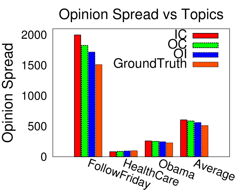
(a) Twitter

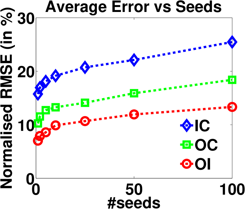
(b) Twitter

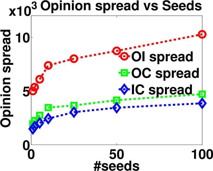
(c) Twitter

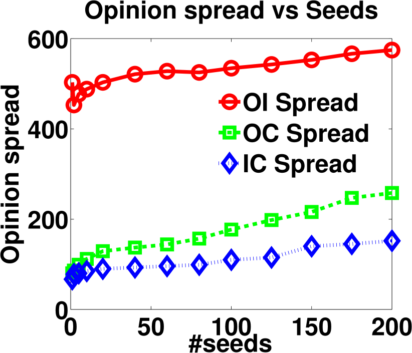
(d) PAKDD

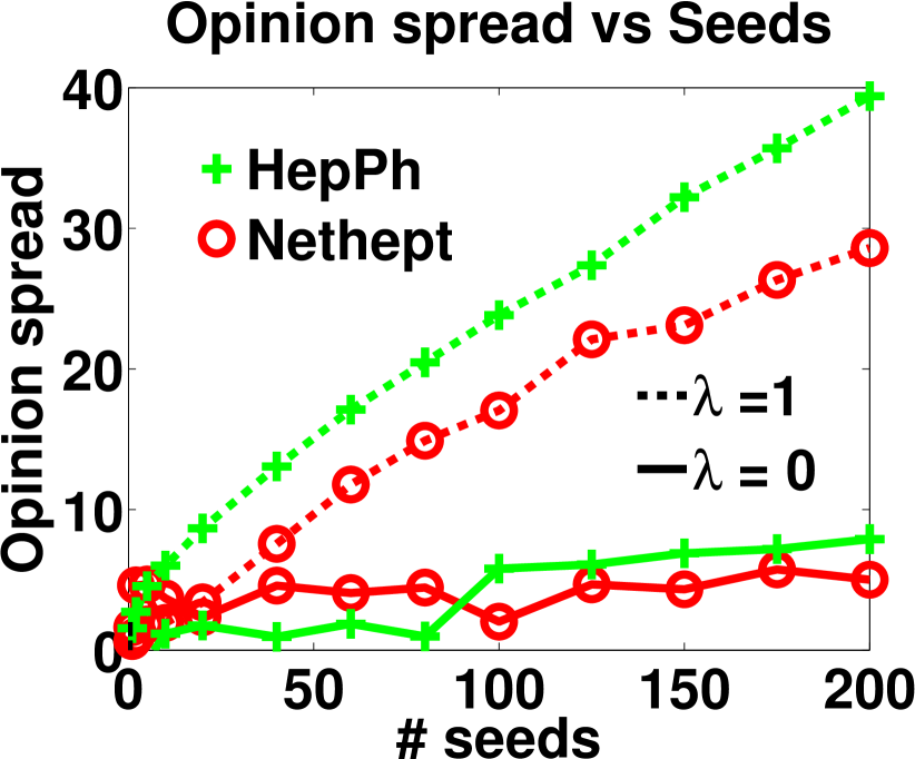
(e) NetHEPT and HepPh

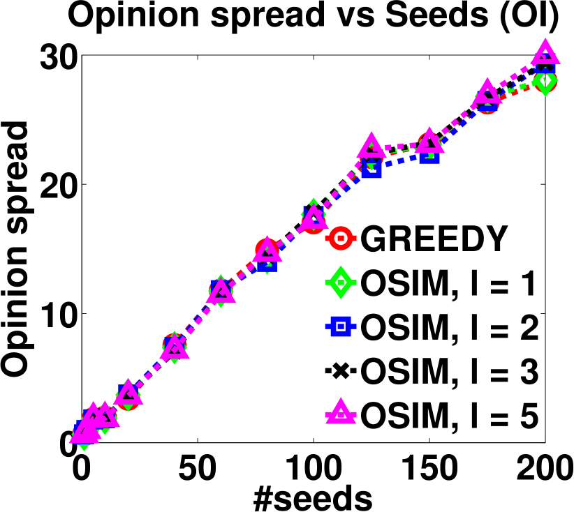
(f) NetHEPT

(g) NetHEPT

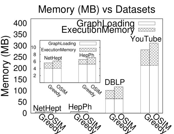
(h) Medium Datasets

Figure 5: Comparison of average opinion-spread under OI, OC and IC with ground-truth for different topic-graphs on Twitter data with (a) k=$50$ seeds and (b) varying seeds. Opinion-spread ($\lambda=1$) comparison of OI with OC and IC on (c) Twitter data and (d) PAKDD data (churn analysis). (e) Opinion-spread comparison of $\lambda=1$ with $\lambda=0$ on NetHept and HepPh. (f) Growth of opinion-spread ($\lambda=1$) with $l$ and $k$ on NetHEPT (OI). (g) Growth-rate of running time with $l$ and $k$ on NetHEPT (OI). (h) Memory consumed for $k=100$ on Medium Datasets.

Comments: Note that we do not perform scalability comparisons of OSIM with the OVM algorithm [48] as (1) Asymptotically, the time complexity of OSIM $\big{(}O(k\mathcal{D}(m+n))$, where $\mathcal{D}$ is a small constant$\big{)}$ is better when compared to OVM $\big{(}O(k^{2}(m+n))\big{)}$, (2) It is rather difficult to extend OVM to work with the OI model and (3) OVM is designed to work with just the LT model at the first-layer while OSIM works with both IC and LT models. Moreover, since the time and space complexity analysis of OSIM is exactly the same as that of EaSyIM, the scalability comparisons performed for the latter serve for the former as well.

4.1 Opinion-Aware

4.1.1 Real Data: Twitter

To motivate the importance of the OI model in real-world scenarios, we employed the use of data extracted from the Twitter social network. This data has two aspects, namely – (1) the underlying (directed) social network, and (2) the tweets by users of this network. A snapshot of the Twitter network, crawled in June $2009$ containing $41.6M$ users (nodes) and $1.5B$ connections (edges), available publicly from [1] is used as the underlying graph. A collection of $476M$ tweets gathered from a subset ($17M$ users) of the users ($41.6M$) in the underlying graph, crawled during the period of June $2009$ to December $2009$, available publicly from [6] constitutes the second part of our dataset. This dataset contains the following information for each tweet, namely – (1) user-id, (2) time-stamp, and (3) the original text message or the tweet.

As discussed in previous sections, the motive of IM, and hence MEO, is to maximize the spread of information about a content, which can be a product, person, event and many more. For instance, in Twitter, the diffusion of information about a topic corresponds to the retweeting of or replying to a tweet or even tweeting about the topic. In fact, the temporal sequence of tweets by users, about a topic, guided by their connections in the network, defines the spread of information about that topic. Thus, as a first step towards analyzing information diffusion in real-world settings, there is a need to extract topic-focussed subgraphs.

To this end, we pre-processed our dataset to retain all the tweets that possess at least one hashtag (#), where hashtags constitute our topics. Thus, we were left with $48.5M$ tweets corresponding to $1.6M$ users. Moreover, we projected the underlying twitter network on this identified subset of $1.6M$ users. This gave us a graph of $1.6M$ users with $75M$ edges among them. We denote this graph with the term background graph in the rest of this section. Moving ahead, we describe the procedure for construction of topic-focussed subgraphs. A topic-focused subgraph evolves by including nodes and edges when users tweet (or retweet) on the same topic, thus (re)activating the edges between them. Following this procedure, we scan the tweets in the increasing order of their time-stamps, and the users associated with the tweets are added as nodes incrementally. Moreover, a directed edge is constructed from a node $A$ to another node $B$ if this edge (directed) exists in the background graph and vice versa. All the nodes with an in-degree of $0$ are considered to be originators or seeds of information. We stop growing a topic-graph if no new seed-nodes were added for a significant amount of elapsed time and start growing a new topic graph. The threshold on the elapsed time was learnt from the data. We look at the average frequency of tweets and identify a time difference as threshold that deviates significantly from the expected. This procedure resulted in $\approx 10$–$12$ topic-focussed subgraphs per hashtag. Note that the construction of topic-focused subgraphs requires just a single scan of the background graph.

Dataset	n	m	Type	Avg. Degree	90-%ile Diameter
NetHEPT	15K	62K	Undirected	4.1	8.8
HepPh	12K	237K	Undirected	19.75	5.8
DBLP	317K	2.1M	Undirected	6.63	8
YouTube	1.13M	5.98M	Undirected	5.29	6.5
SocLiveJournal	4.85M	69M	Directed	14.23	6.5
Orkut	3.07M	234.2M	Undirected	76.29	4.8
Twitter	41.6M	1.5B	Directed	36.06	5.1
Friendster	65.6M	3.6B	Undirected	54.88	5.8

Table 2: Datasets.

With all the data preparation steps in place, next, we use popular sentiment analysis APIs [5, 4] to extract opinions from the tweets. These sources learn a hierarchical classifier, which first determines whether a tweet is neutral or not. Neutral tweets are assigned an opinion score of $0$. If the tweet was not neutral, then another classifier determines the probability of this tweet towards the positive class. Finally, we map this probability value ($[0,1]$) to our opinion scores ($[-1,1]$). Note that the error introduced by the sentiment classifier would equally effect all the following results and thus, it can be safely ignored for all the analsyes.

Next, we show our analyses using topic-focussed subgraphs extracted from high frequency hashtags (top-$100$), each of which possesses at least $50K$ tweets. Unless otherwise stated, the following portrayed results are averaged over all the topic-subgraphs and the normalized root-mean-square error is used as the quality metric. We first show the results of opinion estimation for nodes on unseen topics. The opinions extracted from the tweets of a user, may include the effects of (1) her personal opinion, (2) the influence of her social contacts and (3) external factors. Modelling of external factors is relatively hard from the data, and thus, we consider just the first two factors. As discussed in Sec. 1, we estimate the opinion of a node for a given topic, by considering the opinions of this node for similar topics. Since our topics possess a temporal aspect as well, we estimate the opinion of a node for a topic $A$, by performing a weighted average of the opinion of this node on all the related topics in the past. In addition, since we also possess the true value of the opinion of nodes for the topic $A$, as output by our classifier, we portray the quality of this estimation procedure from our data. We were able to estimate the opinions of the seed-nodes with an error of $3.43\%$ and the opinions of all other nodes with an error of $8.57\%$. Note that the error on non-seed nodes is higher when compared to that on the seed nodes. This is indicative of the fact that the tweets of the seed-nodes indeed express their personal opinion, however the tweets of other nodes additionally include the effect of the opinions of their network. Moreover, this also proves that there is a need for models that: (1) consider the change of opinion during information diffusion, and (2) consider the effect of interaction between two nodes.

Having computed the opinion of each node, the interaction associated with an edge between two nodes (directed) is calculated as the fraction of the times they agree with each other across the subgraphs corresponding to all the topics in the past and not just those corresponding to the related topics. Note that both the parameters for the OI model, namely – opinion and interaction, can be easily computed during the topic-subgraph construction step and do not incur any additional cost for their estimation. As mentioned earlier in this section that topic-subgraph construction is a required step for analyzing information diffusion, thus, the parameter estimation cost for the OI model is amortized constant.

Next, we show that the opinion-spread in real-world follows the OI model. For this experiment, we consider the top-$100$ extracted topic-subgraphs and use the identified seeds or originators of information from the real-world, as the seed nodes for the information diffusion process to measure the opinion spread. For each topic subgraph we calculate the opinion-spread using the opinions extracted from their tweets, which serves as our ground truth. Similarly, we use the estimated parameters on these topic subgraphs and obtain the opinion spread under the OI, OC and the IC models. Although, depending upon the distribution of opinions and interactions, the opinion-spread achieved using all the three models can fall on the either side of the ground-truth, our results in Figure 5a show that the opinion-spread obtained under the OI model is always closest to the ground-truth opinion-spread and thus, possesses the least error. Moreover, Figure 5b shows a similar analysis on the average opinion-spread using the OI, OC and IC models with varying seeds, and it is evident that the opinion-spread under the OI model possesses the least error.

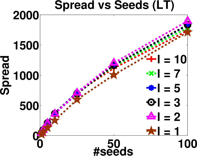
(a) NetHEPT

(b) DBLP

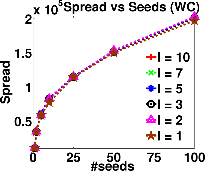
(c) YouTube

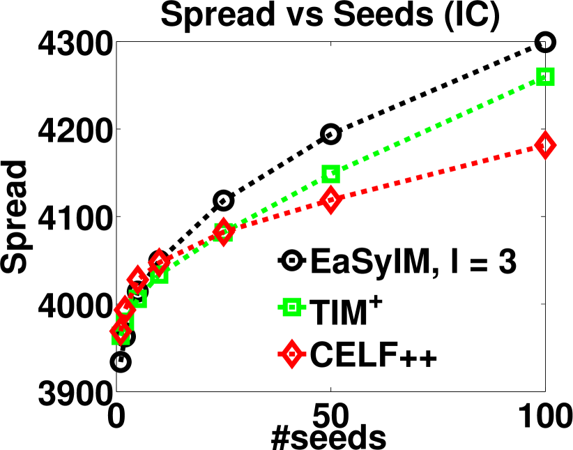
(d) HepPh

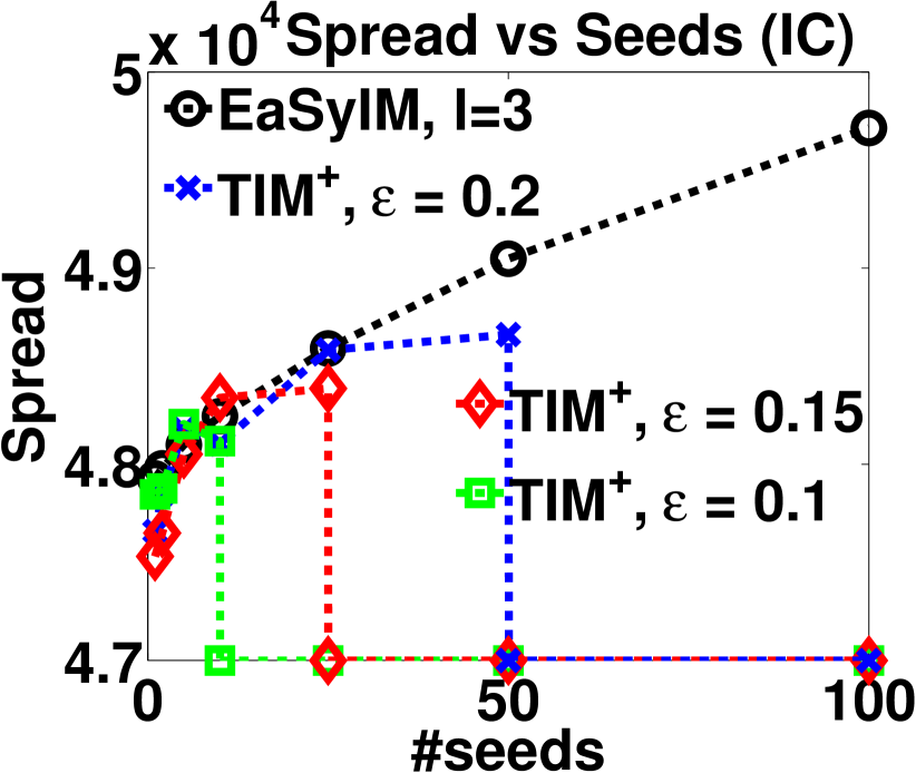
(e) DBLP

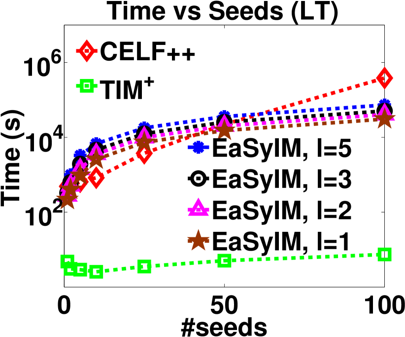
(f) NetHEPT

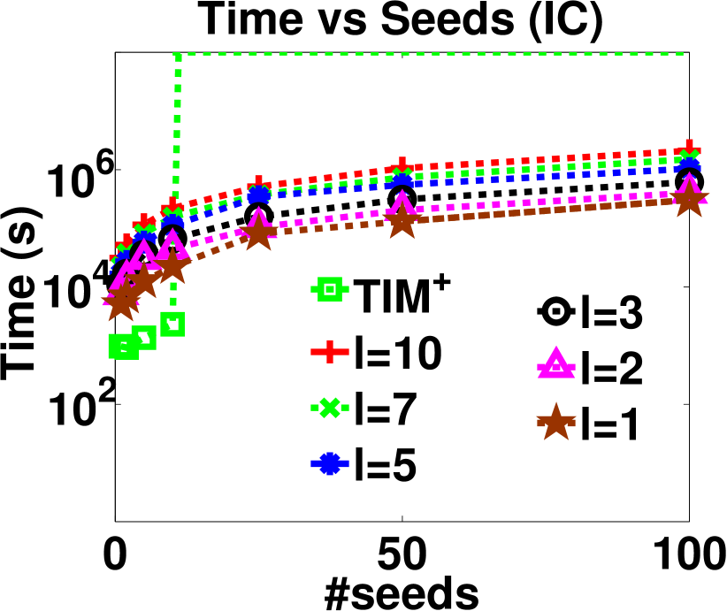
(g) DBLP

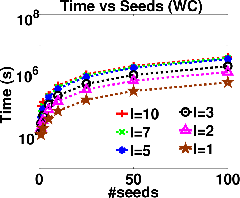
(h) YouTube

(i) NetHEPT and DBLP

(j) Medium Datasets

Figure 6: Growth of spread with $l$ and $k$ on (a) NetHEPT (LT), (b) DBLP (IC) and (c) YouTube (WC). Spread comparison of EaSyIM with TIM⁺ and CELF++ on (e) HepPh (IC), (f) DBLP (IC). Running time comparison of EaSyIM with CELF++ and TIM⁺ on (h) NetHEPT (LT), (i) DBLP (IC) and (j) YouTube (WC). Memory consumption comparison of EaSyIM with CELF++ and TIM⁺ on (m) NetHEPT and DBLP (IC), and with all algorithms for $k=100$ on (n) Medium Datasets (IC).

Having empirically proved that the OI model closely mirrors the opinion-spread in real world scenarios, finally, we show our results on opinion-aware IM. As mentioned earlier in this section, we show the average opinion-spread achieved for different topics by performing the information diffusion process on the entire background graph. Figure 5c shows that the opinion-spread achieved using the seeds selected by the OI model is much better when compared to that of the OC and the IC model. Apart from the results on quality, OSIM with $l=1$, took $497$ minutes and $1.72GB$ of RAM to identify $100$ seeds on the background graph.

4.1.2 Real Data: Analyzing Customer Churn

We used the PAKDD 2012 data mining competition dataset, available publicly from [2], to motivate the applicability of MEO and the OI model in solving real-world problems. The dataset contains profiles of $\approx 100K$ customers, including billing information, usage data, service requests and complaints, of a large telecommunications company for a period of $1$ year from January $1$, $2011$ to December $31$, $2011$. The data also contains information about the churn (termination of services) date for each customer, where $17K$ customers are churners and the rest are non-churners. Using this data, the objective of the challenge was to predict which customers are liable to churn. We extend this problem of modelling customer-churn further to perform a novel analysis using opinion-aware IM. Since the main objective of this paper is not churn-prediction, to make the data preparation step for our analysis simpler we work on a balanced subset of the original data containing $34K$ customers with equal number of churners and non-churners.

Owing to the increasing popularity of label propagation [50] and similarity based learning [20], we build upon the hypothesis that customers with similar attributes possess similar churn behavior. Under this hypothesis, we induce a graph, of customers, using attribute-value similarity and a similarity threshold to construct edges between two customers. The graph obtained thus, consists of $34K$ nodes (customers) and $1.5M$ edges (relationships), with churners assigned a label of $-1$ and non-churners that of $1$. Using this data, we build a model using label-propagation to predict the susceptibility of a customer towards churn. After convergence, the value ($[-1,1]$) at each node represents the affinity, or in other words the opinion, of a customer to churn with $-1$ and $1$ denoting strong affinity towards churn and non-churn respectively. In this way, we estimate the opinion ($o$) parameter of the OI model. The attribute-value similarity defines the influence-proability ($p$) associated with each edge, while the interaction probability ($\varphi$) for each edge is generated using the $rand(0,1)$ function described above.

Acquainted with the likelihood of customers to churn combined with the availability of a churn-prediction model, a service provider would like to identify potential targets, under a marketing buget, capable of maintaining its reputation, thus, indirectly preventing the cascades of churn. This task boils down to identifying seeds that maximize the difference of positive and negative opinions, or in other words maximize the effective opinion (MEO). Figure 5d shows that the opinion-spread achieved using the seeds selected by the OI model is much better when compared to that of the OC and the IC model. This proves the importance of the OI model and the notions of opinion and interaction in solving real-world problems.

4.1.3 Other Real Datasets

Having highlighted the importance of opinion, interaction, the OI model and the MEO problem using two real-world datasets in the previous sections, here we present an in-depth analysis of opinion-aware IM on the benchmark datasets (Table 2) used for the evaluation of classical IM. Since these datasets do not inherently possess the properties of opinion and interaction with nodes and edges of the graph respectively, we annotate them as follows. The opinions are generated by two methods, namely – (a) $o\sim rand(-1,1)$, where the opinion of each node is generated uniformly at random in the range $[-1,1]$ and, (b) $o\sim\mathcal{N}(0,1)$, where the generated opinions follow the standard normal distribution, while the interaction probability for each edge is only generated uniformly and randomly using the function $\varphi\sim rand(0,1)$. The reported results are averaged over $3$ different instances of the generated data. For additional results please see Appendix B.

Quality: The first set of results show the importance of the choice of optimization-objective. We compare the effective opinion-spread ($\lambda=1$) with the opinion-spread ($\lambda=0$) for the NetHEPT dataset using OSIM under the OI model. It is evident from Figure 5e that $\lambda=1$ outperforms $\lambda=0$ and hence, maximizing the effective opinion-spread is better. With this, we fix $\lambda=1$ for a comparison of the effective opinion-spread obtained using OSIM (with varying $l$) with Modified-GREEDY for different datasets. Figure 5f presents the results with varying seeds for NetHEPT under the OI model ($o\sim\mathcal{N}(0,1)$). It can be seen that the reported opinion spread improves with increase in $l$, however, it starts to dip when $l\to\mathcal{D}$ owing to a significant increase in the number of cyclic paths, which in turn causes the error in the assigned scores to increase as discussed in Sec. 3.4.2. Using these results, we conclude that $l=3$ serves as the best choice for OSIM. Moreover, OSIM closely mirrors Modified-GREEDY with respect to the quality of obtained opinion-spread.

Efficiency: In continuation to the comparison on quality, here we compare OSIM with Modified-GREEDY on its running-time for the NetHEPT dataset. Figure 5g shows that OSIM is at least $10^{3}$ times more efficient when compared to Modified-GREEDY with the gain going as high as $10^{5}$ for some cases. Moreover, this figure (with y-axis in log-scale) also shows that the running-time of OSIM grows linearly with increase in $l$.

Scalability: Figure 5h shows a comparison of the memory-consumed by OSIM with Modified-GREEDY for all the $4$ datasets discussed above. It is important to note that the memory consumption of these algorithms is independent of the parameters, namely – path-length ($l$), number of seeds ($k$) and the number of MC simulations. Both the algorithms scale linearly in the size of the graph and require constant-factor overheads to solve the MEO problem. This is indicated by the stacked bars, which show that these algorithms require only a small amount (constant-factor) of memory over and above the memory required to load the graph.

Dataset	Running Time (min)			Memory (MB)
	TIM+	EaSyIM (l=1)	Gain	TIM+	EaSyIM (l=1)	Gain
DBLP	783.1	2183	0.36x	35234.75	46.5	758x
YouTube	NA	5089.5	8	NA	158.3	8
socLive	NA	15433.33	8	NA	974.94	8

Table 3: Comparing EaSyIM with TIM⁺, $k=50$, $\epsilon=0.1$.

As stated earlier, in addition to the scalability and efficiency analysis for OSIM, next, we present a more involved analysis for EaSyIM which serves the purpose for the former as well.

4.2 Opinion-Oblivious

Quality: The first set of results portray the effect of the parameter $l$ on the spread obtained using EaSyIM. Figures 6a, 6b and 6c present the results with varying seeds on the NetHEPT, DBLP and the YouTube datasets under the LT, IC and WC models respectively. It can be seen that the reported spread follows a similar pattern as that of OSIM, i.e., it improves with increase in $l$, however, it starts to dip when $l\to\mathcal{D}$. Using these results, we conclude that $l=5$ serves as the best choice for EaSyIM, with $l=3$ being marginally worse when compared to $l=5$. Moreover, owing to $l=3$ being $\approx 2$ times more efficient when compared to $l=5$ (detailed analysis on efficiency in the following paragraph), we fix $l=3$ for a comparison of the spread obtained using EaSyIM with other algorithms. Figures 6d and 6e present the spreads obtained for the HepPh and DBLP datasets under the IC model. Note that the sudden drop in the spread of TIM⁺ in Figure 6e indicates that it crashed on our machine after that point. These results show that EaSyIM mirrors the state-of-the-art techniques closely for majority of the datasets, while being even better at certain instances, with respect to the quality of the obtained spread.

Efficiency: Figures 6f, 6g and 6h show a comparison of the running-times of EaSyIM with CELF++ and TIM⁺ for varying seeds on the NetHEPT, DBLP and the YouTube datasets under the LT, IC and WC models respectively. These figures show that EaSyIM grows linearly (y-axis in log-scale) with the parameters $l$ and $k$, therefore EaSyIM is $\approx 2$ times faster for $l=3$ when compared to $l=5$. Owing to the marginal improvement in the spread from $l=3$ to $l=5$ (quality analysis in the previous paragraph), we choose $l=3$ for EaSyIM as it provides the best tradeoff between efficiency and quality. Moreover, it can be seen that neither CELF++ nor TIM⁺ scale well with the increase in graph size. CELF++ was not able to complete on the DBLP and the YouTube datasets even after running for $7$ days, while TIM⁺ crashed on the DBLP dataset for $k>10,25,50$ with $\epsilon=0.1,0.15,0.2$ respectively owing to its huge memory requirement. In addition, it is evident from Tables 3 and 4 that EaSyIM is $10$–$15$ times more efficient while consuming $3$-$4$ times less memory when compared to CELF++, and requires $8$–$10$ times more time to run while its memory-footprint is $\approx 500$ times smaller when compared to TIM⁺. We argue that since EaSyIM can be efficiently parallelized owing to the independence of the MC simulations, its lack of efficiency when compared to TIM⁺ can be easily mitigated by running it in parallel on $8$ cores while ensuring the memory gain to be the same.

Scalability: Figure 6i portrays the growth of the memory-footprint of EaSyIM, CELF++, and TIM⁺ with varying seeds for the NetHEPT and the DBLP datasets. It is evident that the memory-consumption of all other techniques, barring TIM⁺ (which grows at a much faster rate), grows linearly with the number of seeds. It is also clear that EaSyIM possesses the smallest memory-footprint, being $\approx 4$ and $\approx 500$ times smaller when compared to CELF++ and TIM⁺ respectively. Moreover, TIM⁺ ($\epsilon=0.1$) crashed for $k>10$ on the DBLP dataset due to going out of memory on our machine. To further this, our experiments revealed that even after relaxing $\epsilon$ to $0.15$ and $0.2$ it crashed for $k>25$ and $k>50$ respectively. This analysis unravels the obvious problem with TIM⁺, i.e., though being efficient it requires an exorbitantly high amount of main-memory and thus, cannot be termed scalable. Figure 6j shows the additional amount of memory required, over and above the memory required to load the graph, by each of our benchmarking algorithms for $4$ different datasets. It is clear that EaSyIM possesses the least overhead while SIMPATH possesses the highest. Note that we omit the bar corresponding to TIM⁺, as it hinders the comparison with other techniques owing to its memory consumption being too high. This shows that EaSyIM possesses the capability of scaling to very large graphs. For additional results please see Appendix B.

Dataset	Running Time (min)			Memory (MB)
	CELF++	EaSyIM (l=1)	Gain	CELF++	EaSyIM (l=1)	Gain
NetHEPT	5352.25	118	45.35x	23.26	3.39	6.86x
HepPh	9746.74	230	41x	24.60	3.47	7.08x
DBLP	NA	5071.67	8	NA	44.73	8

Table 4: Comparing EaSyIM with CELF++, $k=100$ and $l=1$.

In summary, both OSIM and EaSyIM provide the best trade-off between memory-consumption and running-time, and possess the capability to perform IM on large graphs using moderately sized machines or even a laptop.

5 Related Work

The IM problem has been studied extensively over the past decade, thus, it is rather difficult to write a complete literature review in one section. A detailed comparison of the OI model with both IC-N [16] and OC [48], the only other models for opinion-aware IM, has been done qualitatively (Sec. 1) and empirically (Sec. 4). Here, we overview the existing works that overlap with our problem.

(1) Topic-Aware and Competitive IM: The motive of topic-aware IM [11, 8, 15] is to design strategies for maximizing the collective spread of information under a given topic-distribution. It allows different influence probabilities for each topic (assuming a joint distribution of topics), without considering the opinions (of a node) towards these topics. On the other hand, the objective of competitive IM [30, 39, 36] is to maximize the spread of information, about a specific content, in the presence of competitors. It is rather intuitive that competitive IM is similar to topic-aware IM, thus, both of them suffer with same set of deficiencies, i.e., (a) the absence of opinions and negatively activated nodes, and (b) the incapability of capturing their change as information propagates. In addition, another limitation for competitive IM lies with the information-diffusion process, where each node (strictly) propagates information about a particular content and any newly activated node (by the former) also (strictly) follows the same content. In summary, both of them consider maximization of the number of active nodes (opinion-oblivious notion of spread), rendering the spread function to be submodular and thus, are closer to the classical IM problem.

(2) IM in signed networks: IM in signed networks [37] considers the presence of an opinion, from a binary valued set containing exactly opposite opinions, at each node with the notion of friends – capable of activating a node with their own opinion and foes – capable of doing the opposite. The major limitation in this model is the stringent constraint on the parameters to attain values from a discrete binary valued set. On the contrary, OI allows opinions and interactions to come from a real-valued domain. Moreover, the interaction between two nodes is given a probabilistic aspect which is missing in the signed network voter model. In fact, the signed network voter model is rather a special-case of the OI model.

(3) Classical IM: Kempe et al. [32] proved that finding an optimal solution for the IM problem is NP-Hard, and that a simple greedy (GREEDY) algorithm provides the best approximation guarantees in polynomial time. It required $O(kmnr)$ time to produce a solution, where $r$ is the number of MC simulations (usually $r\approx 10K$). This high time complexity renders the GREEDY algorithm inapplicable to the networks of today. Since then, a host of works have introduced optimizations in GREEDY with CELF++ [28] being the most efficient of all within this class of algorithms. Note that these optimizations never improved the asymptotic time complexity of the algorithm. In pursuit of better time complexity, researchers have recently resorted to techniques that use sampling with memoization [13, 46, 23, 45], to portray superior efficiency while retaining approximation guarantees. Among them, TIM⁺ [46], that runs in $O((k+l)(m+n)\log{n}/\epsilon^{2})$ expected time and produces a $(1-\frac{1}{e}-\epsilon)$-approximate solution, where $\epsilon$ is a constant, with probability as high as $1-{n^{-l}}$, and its improvement IMM [45] are the most efficient. Despite their superior efficiency these algorithms lacked scalability, owing to their exorbitantly high memory footprint. The worst case space complexity of TIM⁺ is $O(n^{2}\log{{n\choose k}}/\epsilon^{2})$, which can be very high for small values of $\epsilon$. In addition to the above mentioned techniques, literature has witnessed many heuristic algorithms. Among them, IRIE and SIMPATH [31, 29] are considered state-of-the-art heuristics for the IC and LT models respectively. Although, these techniques build upon a similar idea as that of EaSyIM, its algorithm design and analysis is very different from them with an additional advantage of running in linear space and time. Moreover, as shown in Sec. 4, both of these techniques are not capable of scaling to larger datasets.

6 Conclusions and Future Work

In this paper, we addressed the problem of influence maximization in social networks under a very generic opinion-aware setting, where the nodes can possess any one of the – positive, neutral and negative opinions. To this end, we introduced the novel MEO problem and devised a holistic solution to the influence maximization problem; by coming up with an opinion-cum-interaction (OI) model, and scalable algorithms – OSIM and EaSyIM. Since majority of the works in the literature operate oblivious to the existence of opinions and are not scalable, there are efficiency concerns in real-world scenarios with huge graphs. Consequently, we designed efficient algorithms that run in time linear to the size of the graph. Moreover, the space complexity of our algorithms is also linear; which is orders of magnitude better when compared to the state-of-the-art techniques. Our empirical studies on real-world social network datasets showed that our algorithms are effective, efficient, scale well – providing the best trade-off between running time and memory consumption, and are practical for large real graphs. In future, we would like to come up with a distributed version of our algorithms, thus enabling it scale to even larger graphs.

Acknowledgements: We would like to thank Sayan Ranu, Arnab Bhattacharya, Srikanta Bedathur and Jeff Ullman for providing valuable suggestions and insights throughout the course of this work.

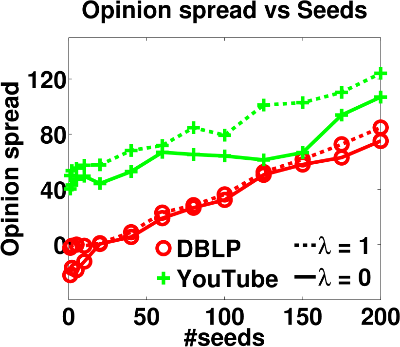
(a) DBLP and YouTube

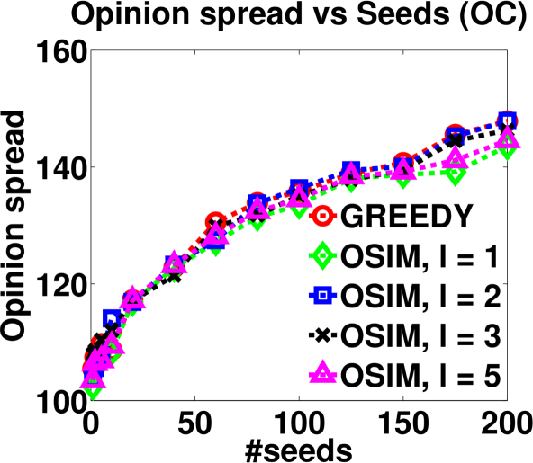
(b) HepPh

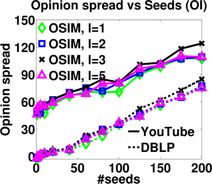
(c) DBLP and YouTube

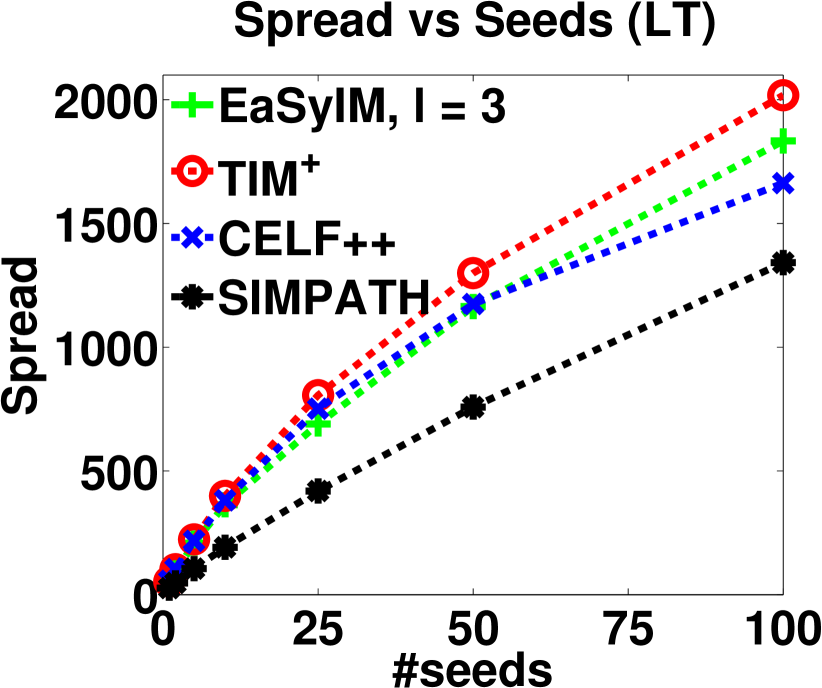
(d) NetHEPT

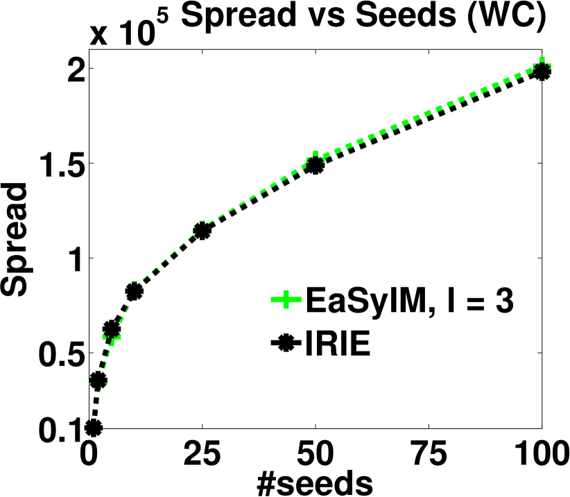
(e) YouTube

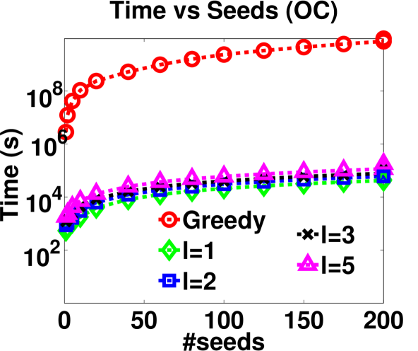
(f) HepPh

(g) DBLP and YouTube

(h) Medium Datasets

(i) Medium Datasets

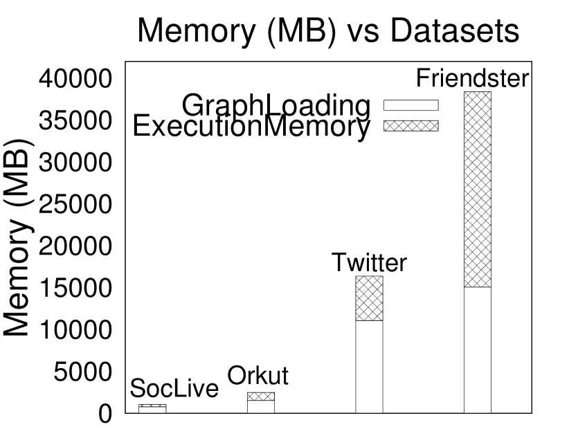
(j) Large Datasets

Figure 7: (a) Opinion-spread comparison of $\lambda=1$ with $\lambda=0$ on DBLP and YouTube. Growth of opinion-spread ($\lambda=1$) with $l$ and $k$ on (b) HepPh (OC), and (c) DBLP and YouTube (OI). Spread comparison of EaSyIM with SIMPATH and IRIE on (d) NetHEPT (LT) and (e) YouTube (WC). Growth-rate of running time of OSIM with $l$ and $k$ on (f) HepPh (OC) and (g) DBLP and YouTube (OI). Running time comparison of EaSyIM with IRIE on (h) Medium Datasets (WC), and SIMPATH on (i) Medium Datasets (LT). (j) Memory consumption of EaSyIM for $k=100$ on Large Datasets.

Appendix A Modified-Greedy Algorithm

Algorithm 6 Modified-GREEDY

0:  Graph $G=(V,E)$,#seeds $k=|S|$

0:  Seed set $S$

1:  $S\leftarrow\emptyset$

2:  for i = 1 to k do

3:     $maxId=\operatorname*{arg\,max}\limits_{w\in V\setminus S}\big{(}\Gamma^{o}_{\lambda}(S\cup\{w\})-\Gamma^{o}_{\lambda}(S)\big{)}$

4:     $S\leftarrow S\cup\{maxId\}$

5:  end for

Appendix B Additional Experimental Results

Quality: It is evident from Figure 7a that $\lambda=1$ outperforms $\lambda=0$ and hence, maximizing the effective opinion-spread is better. Figures 7b and 7c present the results with varying seeds for HepPh under the OC model ($o\sim\mathcal{N}(0,1)$), and DBLP & YouTube under the OI model ($o\sim rand(-1,1)$) respectively. We omit the results for the Modified-GREEDY algorithm in Figure 7c owing to its lack of scalability. Figures 7d and 7e present the spreads obtained for the NetHEPT and YouTube datasets under the LT and WC models respectively.

Efficiency: Figures 7f show that OSIM is at least $10^{3}$ times more efficient when compared to Modified-GREEDY with the gain going as high as $10^{5}$ for some cases. Figure 7g portrays the running time of OSIM for the DBLP and the YouTube datasets. Note that the solid line overlapping with the y-axis and the horizontal top part of the plot shows the time for Modified-GREEDY, which is indicative of the fact that it did not complete even after a month’s time. Figures 7h and 7i show a comparison of the running times of EaSyIM with the state-of-the-art heuristics – IRIE (WC) and SIMPATH (LT). It is evident that both of these techniques do not scale well. EaSyIM is $2-3$ and $4-6$ times faster when compared to IRIE for small and medium sized datasets respectively. It is slower when compared to SIMPATH on smaller datasets, however, highly efficient for the medium sized datasets as SIMPATH did not complete even after $5$ days on the DBLP dataset.

Scalability: Eventually as a part of our scalability experiments, we present the memory required by EaSyIM for the $4$ large graph datasets (Table 2) in Figure 7j. This shows that EaSyIM possesses the capability of scaling to graphs with billion-scale edges.

Appendix C Additional Note on CELF++

This algorithm exploits the sub modularity of the problem by using a “lazy-forward” optimization while selecting seeds. This technique calculates marginal gain of nodes in decreasing order of their probability of being a seed node, which in turn is calculated form its marginal gain in previous iterations. Another optimization which helped engineer the running time of this algorithm was to ignore the nodes which do not hold a chance to become a seed node in consequent iterations.

References

- [1] http://an.kaist.ac.kr/traces/WWW2010.html.
- [2] http://lamda.nju.edu.cn/zhangt/dm2012/Project4.html.
- [3] arXiv. http://www.arxiv.org.
- [4] Empath: Sentiment, Topic, and Demographic Analysis. https://www.parc.com/services/focus-area/bigdata/.
- [5] Natural Language Sentiment Analysis API. http://text-processing.com/demo/sentiment/.
- [6] SNAP Datasets. https://snap.stanford.edu/data/.
- [7] The Boost Graph Library. http://www.boost.org.
- [8] Ç. Aslay, N. Barbieri, F. Bonchi, and R. A. Baeza-Yates. Online topic-aware influence maximization queries. In EDBT, pages 295–306, 2014.
- [9] C. Aslay, W. Lu, F. Bonchi, A. Goyal, and L. V. S. Lakshmanan. Viral marketing meets social advertising: Ad allocation with minimum regret. PVLDB, 8:814–825, 2015.
- [10] L. Backstrom, D. Huttenlocher, J. Kleinberg, and X. Lan. Group formation in large social networks: Membership, growth, and evolution. In KDD, pages 44–54, 2006.
- [11] N. Barbieri, F. Bonchi, and G. Manco. Topic-aware social influence propagation models. In ICDM, pages 81–90, 2012.
- [12] N. Barbieri, F. Bonchi, and G. Manco. Cascade-based community detection. In WSDM, pages 33–42, 2013.
- [13] C. Borgs, M. Brautbar, J. Chayes, and B. Lucier. Maximizing social influence in nearly optimal time. In SODA, pages 946–957, 2014.
- [14] V. Chaoji, S. Ranu, R. Rastogi, and R. Bhatt. Recommendations to boost content spread in social networks. In WWW, pages 529–538, 2012.
- [15] S. Chen, J. Fan, G. Li, J. Feng, K.-l. Tan, and J. Tang. Online topic-aware influence maximization. PVLDB, 8:666–677, 2015.
- [16] W. Chen, A. Collins, R. Cummings, T. Ke, Z. Liu, D. Rincon, X. Sun, Y. Wang, W. Wei, and Y. Yuan. Influence Maximization in Social Networks When Negative Opinions May Emerge and Propagate. In SDM, 2011.
- [17] W. Chen, C. Wang, and Y. Wang. Scalable influence maximization for prevalent viral marketing in large-scale social networks. In KDD, pages 1029–1038, 2010.
- [18] W. Chen, Y. Wang, and S. Yang. Efficient influence maximization in social networks. In KDD, pages 199–208, 2009.
- [19] W. Chen, Y. Yuan, and L. Zhang. Scalable influence maximization in social networks under the linear threshold model. In ICDM, pages 88–97, 2010.
- [20] Y. Chen, E. K. Garcia, M. R. Gupta, A. Rahimi, and L. Cazzanti. Similarity-based classification: Concepts and algorithms. Journal of Machine Learning Res, 10:747–776, 2009.
- [21] S. Cheng, H. Shen, J. Huang, W. Chen, and X. Cheng. Imrank: influence maximization via finding self-consistent ranking. In SIGIR, pages 475–484, 2014.
- [22] S. Cheng, H. Shen, J. Huang, G. Zhang, and X. Cheng. Staticgreedy: solving the scalability-accuracy dilemma in influence maximization. In CIKM, pages 509–518, 2013.
- [23] E. Cohen, D. Delling, T. Pajor, and R. F. Werneck. Sketch-based influence maximization and computation: Scaling up with guarantees. In CIKM, pages 629–638, 2014.
- [24] T. N. Dinh, H. Zhang, D. T. Nguyen, and M. T. Thai. Cost-effective viral marketing for time-critical campaigns in large-scale social networks. IEEE/ACM Trans. Netw., 22:2001–2011, 2014.
- [25] S. Eubank, H. Guclu, V. S. Anil Kumar, M. V. Marathe, A. Srinivasan, Z. Toroczkai, and N. Wang. Modelling disease outbreaks in realistic urban social networks. Nature, 429(6988):180–184, 2004.
- [26] S. Galhotra, A. Arora, S. Virinchi, and S. Roy. Asim: A scalable algorithm for influence maximization under the independent cascade model. In WWW (Companion Volume), 2015.
- [27] H. Gao, J. Mahmud, J. Chen, J. Nichols, and M. X. Zhou. Modeling user attitude toward controversial topics in online social media. In ICWSM, 2014.
- [28] A. Goyal, W. Lu, and L. V. Lakshmanan. Celf++: Optimizing the greedy algorithm for influence maximization in social networks. In WWW (Companion Volume), pages 47–48, 2011.
- [29] A. Goyal, W. Lu, and L. V. Lakshmanan. Simpath: An efficient algorithm for influence maximization under the linear threshold model. In ICDM, pages 211–220, 2011.
- [30] X. He, G. Song, W. Chen, and Q. Jiang. Influence blocking maximization in social networks under the competitive linear threshold model. In SDM, pages 463–474, 2012.
- [31] K. Jung, W. Heo, and W. Chen. Irie: Scalable and robust influence maximization in social networks. In ICDM, pages 918–923, 2012.
- [32] D. Kempe, J. Kleinberg, and E. Tardos. Maximizing the spread of influence through a social network. In KDD, pages 137–146, 2003.
- [33] J. Kim, S.-K. Kim, and H. Yu. Scalable and parallelizable processing of influence maximization for large-scale social networks? In ICDE, pages 266–277, 2013.
- [34] J. Leskovec, J. Kleinberg, and C. Faloutsos. Graphs over time: Densification laws, shrinking diameters and possible explanations. In KDD, pages 177–187, 2005.
- [35] J. Leskovec, A. Krause, C. Guestrin, C. Faloutsos, J. VanBriesen, and N. Glance. Cost-effective outbreak detection in networks. In KDD, pages 420–429, 2007.
- [36] H. Li, S. S. Bhowmick, J. Cui, Y. Gao, and J. Ma. Getreal: Towards realistic selection of influence maximization strategies in competitive networks. In SIGMOD, pages 1525–1537, 2015.
- [37] Y. Li, W. Chen, Y. Wang, and Z.-L. Zhang. Influence diffusion dynamics and influence maximization in social networks with friend and foe relationships. In WSDM, pages 657–666, 2013.
- [38] K. W. Lim and W. Buntine. Twitter opinion topic model: Extracting product opinions from tweets by leveraging hashtags and sentiment lexicon. In CIKM, pages 1319–1328, 2014.
- [39] W. Lu, F. Bonchi, A. Goyal, and L. V. S. Lakshmanan. The bang for the buck: fair competitive viral marketing from the host perspective. In KDD, pages 928–936, 2013.
- [40] Y. Mehmood, N. Barbieri, F. Bonchi, and A. Ukkonen. CSI: community-level social influence analysis. In ECML/PKDD, pages 48–63, 2013.
- [41] G. Nemhauser, L. Wolsey, and M. Fisher. An analysis of approximations for maximizing submodular set functions—i. Mathematical Programming, 14(1):265–294, 1978.
- [42] N. Ohsaka, T. Akiba, Y. Yoshida, and K. Kawarabayashi. Fast and accurate influence maximization on large networks with pruned monte-carlo simulations. In AAAI, pages 138–144, 2014.
- [43] A. Pak and P. Paroubek. Twitter as a corpus for sentiment analysis and opinion mining. In LREC, 2010.
- [44] M. Richardson and P. Domingos. Mining knowledge-sharing sites for viral marketing. In KDD, pages 61–70, 2002.
- [45] Y. Tang, Y. Shi, and X. Xiao. Influence maximization in near-linear time: A martingale approach. In SIGMOD, pages 1539–1554, 2015.
- [46] Y. Tang, X. Xiao, and Y. Shi. Influence maximization: Near-optimal time complexity meets practical efficiency. In SIGMOD, pages 75–86, 2014.
- [47] L. G. Valiant. The complexity of enumeration and reliability problems. SIAM Journal on Computing, 8:410–421, 1979.
- [48] H. Zhang, T. N. Dinh, and M. T. Thai. Maximizing the spread of positive influence in online social networks. In ICDCS, pages 317–326, 2013.
- [49] X. W. Zhao, Y. Guo, Y. He, H. Jiang, Y. Wu, and X. Li. We know what you want to buy: A demographic-based system for product recommendation on microblogs. In KDD, pages 1935–1944, 2014.
- [50] X. Zhu and Z. Ghahramani. Learning from labeled and unlabeled data with label propagation.