The Formation Mass of a Binary System via Fragmentation of a Rotating Parent Core with Increasing Total Mass

Abstract

Recent VLA and CARMA observations have shown proto-stars in binaries with unprecedented resolution. Specifically, the proto-stellar masses of systems such as CB230 IRS1 and L1165-SMM1 have been detected in the range of $0.1-0.25\,M_{\odot}$. These are much more massive than the masses generally obtained by numerical simulations of binary formation, around $0.01\,M_{\odot}$. Motivated by these discrepancies in mass, in this paper we study the formation mass of a binary system as a function of the total mass of its parent core. To achieve this objective, we present a set of numerical simulations of the gravitational collapse of a uniform and rotating core, in which azimuthal symmetric mass seeds are initially implemented in order to favor the formation of a dense filament, out of which a binary system may be formed by direct fragmentation. We first observed that this binary formation process is diminished when the total mass of the parent core $M_{0}$ is increased; then we increased the level of the ratio of kinetic energy to the gravitational energy, denoted by $\beta$, initially supplied to the rotating core, in order to achieve the desired direct fragmentation of the filament. Next, we found that the mass of the binary fragment increases with the mass of the parent core, as expected. In this paper we confirm this expectation and also measure the binary mass $M_{f}$ obtained from an initial $M_{0}$. We then show a schematic diagram $M_{0}$ vs $\beta$, where the desired binary configurations are located while the ratio of the thermal energy to the gravitational energy $\alpha$ is kept fixed. We also report some basic physical data of the proto-stellar fragments that form the binary system, including the formation mass $M_{f}$, and its corresponding $\alpha_{f}$ and $\beta_{f}$. Finally, we show the resulting velocity distribution for our calculated models.

keywords:–stars: formation;–physical processes: gravitational collapse, hydrodynamics;–methods: numerical

1 Introduction

The formation of low mass-star binaries is well-understood with regard to its basic physical principles; see [Boden 2011] and [Stahler & Palla 2004]. The essential events of this formation process are the gravitational collapse of cores and their fragmentation during an early evolution stage of the collapsing cores; see [Reipurth et al 2002], [Duchêne et al 2004] and [Girart et al 2004].

As for the observational aspect, recent technical improvements have made it possible to improve the spatial resolution and observe a few protostars in their Class 0 evolution stage; for instance, L1157-mm, CB230 IRS1 and L1165-SMM1, all isolated and located in the Cepheus Flare region; see [Tobin at al. 2013]; there was less evidence of direct observation of a disk, for instance, that with radius 125 AU surrounding the protostar L1527; see [Tobin et al. 2012]. However, spatial resolutions better than 50 AU are needed in order to produce basic physical information and provide clues regarding the mechanisms of binary system formation.

For the Taurus dark cloud, a correlation between the mass of the newly formed stars and the mass of the associated dense proto-stellar cores in the cloud was observed long ago by  [Myers 1983].

With regard to the theoretical aspect, numerical simulations aimed at reproducing the collapse of rotating cores began to be performed four decades ago. The most well-known example of isothermal fragmentation during a core collapse was first calculated by [Boss & Bodenheimer 1979]. This model is now called the ”standard isothermal test case” as it has been used for testing new codes and making code comparisons. The outcome of this classic model and of a variant of thereof calculated by [Burkert & Bodenheimer 1993] and [Bate & Burkert 1997] was a protostellar binary system.

The earliest papers on collapse were largely done with insufficient spatial resolution; see for instance [Boss 1991], therefore, these calculations suffered from artificial fragmentation due to violation of the Jeans condition; see [Truelove et al. 1997]. Nowadays, a new generation of three-dimensional collapse calculations have improved so much in resolution, that they now reveal, in very valuable detail, the formation of a binary system or multiple systems of low mass proto-stars by starting with a density perturbation with azimuthal symmetry that was successfully implemented long ago by [Boss et al. 2000]; see [Truelove et al 1998], [Klein et al 1999], [Boss et al. 2000], [Kitsionas & Whitworth 2002] and [Springel 2005]. Many of these numerical experiments were done using a solar mass parent core, that collapsed under its self-gravity against its thermal pressure and rotational support to form a binary system composed of very low mass proto-stars; see the review by [Tohline 2002]. However, taking advantage of scaling relations valid in a nearly homologous isothermal collapse, [Sterzik et al. 2003] demonstrated that the final properties of the binary system depend on the initial conditions of the parent core, such as its temperature, mass and angular momentum. The assumption of isothermality allows for the existence of such scaling relations, so that the results obtained for the collapse of a one solar mass parent core can be scaled to cores of arbitrary mass only in the isothermal regime.

Recent VLA and CARMA observations have shown proto-stars in binaries with unprecedented resolution. Specifically, the proto-stellar masses of systems such as CB230 IRS1 and L1165-SMM1 have been detected in the range of $0.1-0.25\,M_{\odot}$. These are much more massive than the masses generally obtained by numerical simulations of binary formation, with an initial fragment mass of around $0.01\,M_{\odot}$, when the calculations must be stopped because of insufficient spatial resolution and small time steps. The fragments will accrete mass and continue to grow so long as infalling gas is available. Motivated by these discrepancies in mass, in this paper we study the formation mass of a binary system as a function of the total mass of its parent core. To achieve this objective, in this paper we present high-resolution three-dimensional hydrodynamical simulations, done with the public code Gadget2, which implements the SPH technique, in order to follow the gravitational collapse of a uniform and rotating core in a variant of the standard test case, in which we implemented a mass perturbation, with the same mathematical structure as the density perturbation used by [Boss et al. 2000], to enforce the formation of two antipode embryonic binary mass seeds during the early core collapse. This system evolved to a pair of well-defined mass condensations connected by a dense filament.

In this intermediate evolution stage of the core collapse, two events may take place according to the assembled mass of these mass condensations. If the assembled mass is low enough for the centrifugal force (due to core rotation) to overcome the gravitational attraction of the mass condensations, then they approach each other, achieve rotational speed, swing past each other and finally separate to form the desired fragments, which will become the binary system, in which the fragments orbit around one another. When the condensed masses are massive enough, then they approach each other, make contact and merge to form a single central proto-stellar mass condensation.

When the total mass of the parent core $M_{0}$ is increased, the merging event is thus favored while the binary formation process is diminished. The formed single central mass condensation is surrounded by a disk out of which two additional small mass condensations may be formed by disk fragmentation, so that this kind of simulation ends with a multiple system, dominated by a primary mass. These kind of configurations were obtained by [Hennebelle et al 2004] by increasing the external pressure on a rotating core. To prevent the occurrence of merging, we increased the ratio of rotational energy to gravitational energy, $\beta$, supplied initially to the parent core, while we kept the ratio of thermal energy to potential energy, $\alpha$, fixed for our all simulations. [Matsumoto & Hanawa 2003] and [Tsuribe 2002] studied the effects of different rotation speeds and rotation laws on the fragmentation of a rotating core. These authors introduced six types of fragmentation seen as the possible outcomes of a collapsing core. The configuration that interests us in this paper corresponds to their disk-bar type fragmentation. They also showed a configuration diagram whose axes were given by products of the free fall time $t_{ff}$ measured from the central density, multiplied by the initial central angular velocity $\Omega_{0}$, and the amplitude of the velocity perturbation of the $m=2$ mode $\Omega_{2}$, respectively.

To start our study, we arbitrarily chose two initial $\beta$ ratios: the lower value given by $\beta=0.045$ and the higher value given by $\beta=0.14$, while we fixed $\alpha=0.24$. The number of Jeans masses contained in a uniform spherical core is given by $1/\alpha$. Thus the number of fragments that we expect to form is 2. We thus constructed a schematic diagram the axis of which were $M_{0}$ and the measured $\beta$, where we showed the kind of configuration obtained: either primary or the desired binary. It is important to note that recent observations made by [Tokovin 2000] seem to confirm the existence of dwarf binaries with mass ratios $q=M_{2}/M_{1}$ from 0.95 to 1, as first described by [Lucy & Ricco 1979]; some examples of this kind of system are MM Her and EZ Peg, with $q$ given by 0.98 and 0.99, respectively. The particular mechanism of fragmentation considered in this paper can be potentially useful as a template for studying binary systems with $q$ close to 1.

Furthermore, as the parameter space relevant to the core collapse is so large, it is not easy to anticipate the outcome of a given collapse simulation. A first effort for establishing a criterion of the type $\alpha\,\beta<0.2$, for predicting the occurrence of fragmentation of a rotating isothermal core was obtained by means of numerical simulations by [Miyama et al 1984], [Hachisu & Heriguchi 1984] and [Hachisu & Heriguchi 1985]. Furthermore, [Tsuribe et al. 1999] made a semi-analytical study to construct a configuration space whose axes were the dimensionless quantities $\alpha$ and $\beta$. [Tsuribe 2002] introduced another fragmentation criterion based on the flatness of the core, such that the configuration diagrams $\alpha$ versus $\beta$ were improved. It must be emphasized that numerical simulations seem to prove that these fragmentation criteria can only provide a clue regarding the fate of a specific initial core configuration but can-not predict its exact outcome or the number of fragments that may be produced during its gravitational collapse.

According to these fragmentation criteria, the values for $\alpha$ and $\beta$ that we use in this paper favor the collapse of the core and the formation of the embryonic binary system according to [Tsuribe et al. 1999], but it is not still clear what the next events are, as they depend on the assembled mass, as we mentioned in a previous paragraph. So, we performed numerical simulations in order to determine exactly the main simulation outcome beyond the formation of the mass condensations.

In the early simulations on the collapse of rotating cores, the ideal equation of state was used as a first approximation. However, once that gravity produces a substantial contraction of the core, the gas begins to heat. In order to take this heating into account, in our simulations we implemented a barotropic equation of state beos, as was proposed by [Boss et al. 2000]. The beos depends on a single free parameter, the critical density $\rho_{crit}$. [Arreaga et al. 2008] reported a study of the effects of the change in the thermodynamic regime on the outcome of a particle-based simulation, where several values of the critical density were considered. The simulations that we present here increased the peak density up to three orders of magnitude within this adiabatic regime. Therefore, the scaling relations obtained under the assumption of isothermality are no longer valid for this final evolutionary stage of our simulations.

The outline of this paper is as follows: the basic physics of the core and the particle distribution that represents the initial core are described in Section 2. The most important features of the time evolution of these simulations are presented by means of 2D iso-density plots in Section 3. The relevance of these results in view of those reported in previous works is discussed in Section 4. Furthermore, we show the velocity distribution obtained for the binaries by means of iso-velocity 3D plots in Section4.3. Finally, some concluding remarks are made in Section 5.

2 The core

We consider a spherical core with radius $R_{0}=4.99\,\times 10^{16}$ cm $\equiv\,3335\,$ AU, which is rigidly rotating around the $z$ axis with an angular velocity $\Omega$, so that the initial velocity of the $i-th$ SPH particle is given by $\vec{v}_{i}=\vec{\Omega}\times\vec{r}_{i}\equiv(-\Omega\,y_{i},\Omega\,x_{i},0)$.

In Section 3 we will present the results of several simulation models where the total core mass is systematically increased up to $5\,\,M_{\odot}$. We emphasize that we left the initial core radius unchanged, so that the average density increased instead. However, these models still correspond to a core, as defined statistically by [Bergin & Tafalla 2007].

The time needed for a test particle to reach the center of the core when gravity is the only force acting on it, is defined as the free fall time $t_{ff}$ by means of

$$t_{ff}=\sqrt{\frac{3\,\pi}{32\,G\,\rho_{0}}}$$ (1)

where $\rho_{0}=3.8\,\times 10^{-18}\,$ g cm^-3 is the average density of a $1\,M_{\odot}$ core with radius $R_{0}$. These values of $t_{ff}$ and $\rho_{0}$ are used as normalizing factors for the plots presented below.

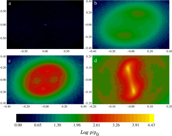
Figure 1: Iso-density plot to show the early evolution of all the models.

2.1 The radial mesh for core particles

We used an initial grid with spherical geometry, so that a set of concentric shells were created and populated with SPH particles in the following sense. We divided the total volume $V$ of the sphere of radius $R_{0}$ into a given number of bins, $N_{bin}$, such that $\Delta V=V/N_{bin}$ is the volume of a spherical shell. Each shell can be characterized by a radial interval $(r_{l},r_{f})$, such that its initial and final radius are $r_{l}$ and $r_{f}$, respectively. The radius $r_{f}$ is determined by the condition that $\Delta V$ be constant. Hence, we have

$$r_{f}=\left(r_{l}+\frac{\Delta V}{4\pi/3}\right)^{1/3}.$$ (2)

Thus, the first shell is determined by the radial interval $(0,r_{1})$, while the second shell is delimited by $(r_{1},r_{2})$, and so on. Let us now define the average radius $r_{s}$ and the radial width of a given shell as $r_{s}=(r_{l}+r_{f})/2$ and $\delta_{s}=(r_{f}-r_{l})$, respectively.

Then, by means of a Monte Carlo scheme, we populated each concentric shell with a given number of equal mass particles, $N_{par}$, so that the particles were located randomly in all the available surfaces of each spherical shell. The spherical coordinates of the particles of a given shell $(r_{s},\theta,\phi)$ are related to uniform random variables $u$ and $v$ (taking real values within the interval $[0,1]$) by the following equations:

$$\begin{array}[]{l}u=\frac{1-\cos(\theta)}{2}=\frac{1}{2}\int_{0}^{\theta}\sin(\theta^{\prime})\,d\theta^{\prime}\,,\vspace{0.1 cm}\\ v=\frac{\phi}{2\pi}=\frac{1}{2\,\pi}\int_{0}^{\phi}\,d\phi^{\prime}\end{array}$$ (3)

We thus have a total of $N_{bin}\,\times\,N_{par}$ particles distributed in the spherical volume of the core, such that the total mass in each shell is constant and given by $N_{par}\,m_{0}$, where $m_{0}$ is the particle mass, so that the global density of the core is also constant. To achieve a constant density distribution in a local sense, we further applied a radial perturbation to all the particles of a given shell such that any particle could be randomly displaced radially outward or inward, but preventing a perturbed particle from reaching another shell. The radial perturbations $\epsilon_{r}$ applied to each SPH particle, regardless of the model, were at the order of $\epsilon_{r}=\delta_{s}/2$.

In the first panel of Fig.1, one can appreciate the spherical nature of the initial mesh, as only the innermost radial shell is visible due to the huge contrast in density between this and the outer shells.

In all the simulations of this paper, we used a total of two million SPH particles, which according to the convergence study done by [Arreaga et al. 2007], is high enough to fulfill the resolution requirements described by [Truelove et al. 1997].

2.2 Mass perturbation

We ensured that a binary system would be formed in the simulation by implementing a mass perturbation such that, if $m_{0}$ is the particle mass, the perturbed mass $m_{i}$ of particle $i$ is $m_{i}=m_{0}+m_{0}*a\cos\left(m\,\phi_{i}\right)$, where the perturbation amplitude is set to $a=0.1$ and the mode is fixed at $m=2$; $\phi$ is the azimuthal spherical coordinate.

There are other methods for the implementation of density perturbations, such as the Monte Carlo scheme, in which the particle mass remains unchanged. Nevertheless, the mass perturbation we implemented here was successfully applied in our previous papers on collapse; see [Arreaga et al. 2007] and [Arreaga et al. 2008], and remarkably also for other authors, such as [Springel 2005]. With particle mass variations within ten percent of the initial particle mass, as is the case of our simulations, there are no border or particle deficiency effects to worry about.

2.3 The barotropic equation of state

To take into account the heating of the gas due to both core contraction and energy dissipation from artificial viscosity, we used the barotropic equation of state proposed by [Boss et al. 2000]:

$$p=c_{0}^{2}\rho\left[1+\left(\frac{\rho}{\rho_{crit}}\right)^{\gamma-1}\right]$$ (4)

where $\gamma=5/3$ and $c_{0}$ is the sound speed so that the corresponding temperature associated with the gas core is $T\approx 10\,$K. The critical density $\rho_{crit}$ determines the change in the thermodynamic regime from isothermal to adiabatic. For the early phases of the collapse, when the peak density is much lower than the critical density, $\rho_{max}<<\rho_{crit}$, the beos becomes an ideal equation of state; for the late phases of the collapse, when $\rho_{max}>>\rho_{crit}$, there is an increase in pressure according to $p\approx\rho^{3/2}$, then the beos becomes an adiabatic relation.

We use only one value given by $\rho_{crit}=5.0\times 10^{-14}\,$ g cm^-3. As we will show in the following sections, in the simulations considered in this paper, the average peak density reached ranges around $\rho=2.5\times 10^{-11}\,$ such that the core density increased up to 3 orders of magnitude within the adiabatic regime.

3 Results

Table 1: The models and their main results.

Model	$M/M_{\odot}$	$\beta$	$t_{max}/t_{ff}$	$log_{10}\left(\rho_{max}/\rho_{0}\right)$	Configuration
m075b0045	0.75	0.045	1.29	7.50	Binary
m075b014	0.75	0.14	1.57	6.78	Binary
m1b0045	1.0	0.045	1.11	7.28	Binary
m1b014	1.0	0.14	1.38	6.79	Binary
m1p5b0045	1.5	0.045	0.937	6.99	Primary
m1p5b011	1.5	0.11	1.08	6.94	Binary
m1p5b014	1.5	0.14	1.10	6.70	Binary
m2p5b0045	2.5	0.045	0.76	7.02	Primary
m2p5b013	2.5	0.13	0.87	6.83	Binary
m2p5b014	2.5	0.14	0.83	6.62	Binary
m5b0045	5.0	0.045	0.53	6.58	Primary
m5b014	5.0	0.14	0.71	7.73	Primary
m5b021	5.0	0.21	0.71	6.47	Binary

Figure 2: Time evolution of the peak density.

Worldwide simulations performed in order to follow the collapse of a uniform density core have proven that an isolated rotating core contracts itself to an almost flat configuration approximately within a free-fall time of dynamical evolution; see for instance [Bodenheimer et al. 2000], [Sigalotti & Klapp 2001] and the references therein. Therefore, in order to illustrate our results, we used $2D$ iso-density plots for a slice of particles around the equatorial plane of the core.

Let us now emphasize some important features of the early evolution of the collapsing core, where the mass perturbation mentioned in Section 2.2 plays a fundamental role. When the peak density reaches a value around $1.0\,\times 10^{-16}\,$g cm^-3, the mass perturbation generates two well-defined mass condensations, which are clearly visible in the second panel of Fig.1. These mass condensations act as mass attraction centers. As more mass is being accreted by these centers, the peak density monotonically increases on them and in their surroundings as well, as can be noted by the color scale acquired by the central region of the core in the third and fourth panels of Fig.1, respectively. Thus, all the models considered here finish this first evolution stage with an embryonic binary system composed by two well-defined mass condensations connected by a filament.

As can be seen in Fig. 2, our simulations easily satisfy some basic expectations, some of which are: (i) all the models collapse by the end of the simulation; (ii) the larger the value of $\beta$ given initially to the core, the slower the core collapses; (iii) the more massive the initial core, the faster it collapses; (iv) there must be a maximum $\beta$ value, so that for $\beta>\beta_{max}$, the core simply expands without contracting.

First, there are two competing forces that determine the next events to occur in the central core: on one hand, the gravitational force, so that each mass condensation pulls on the other, favoring their approach; on the other hand, centrifugal force, acting on each mass condensation favoring their separation.

Now we shall separately illustrate the results of each model by means of colored iso-density figures. In Table 1 we summarize the considered models and their main results, according to the following entries: column one gives the label and column two shows the total mass of the parent core; in column three we give the $\beta$ initially provided to the core, while the maximum evolution time and peak density of the simulation are shown in the fourth and fifth columns, respectively; finally, the last column shows the configuration obtained, either binary or primary, as explained below.

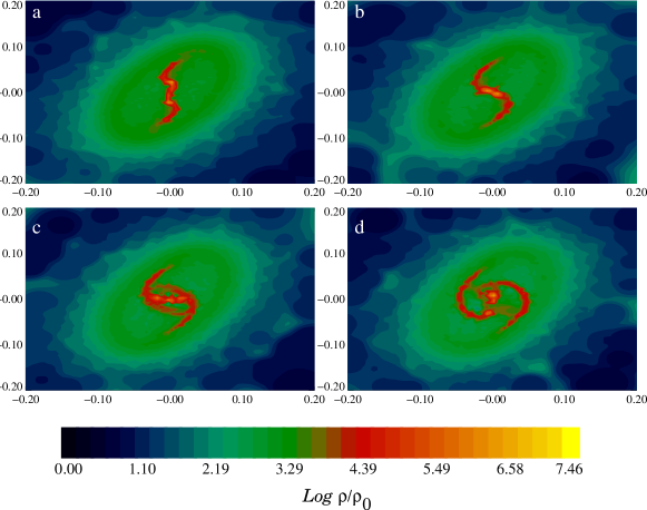
Figure 3: Iso-density plot for model m0p75b0045.

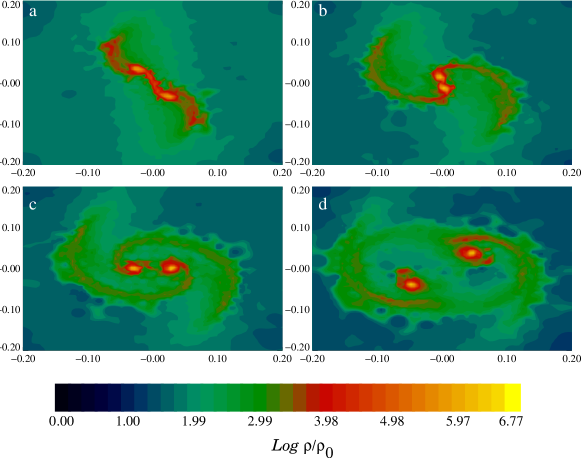
Figure 4: Iso-density plot for model m0p75b014.

3.1 Models with parent core mass up to $M_{0}=1\,M_{\odot}$

The models considered in this section are those labeled with m075 and m1 in Table 1. For all these models, the gravitational attraction between the formed mass condensations is very easily overcome by the centrifugal repulsion; then the mass condensations avoid the contact between them and fly apart to become truly fragments which enter in orbit around one another, so we obtained the desired binary configurations.

The iso-density plots for the low and high $\beta$ models with $M_{0}=0.75\,M_{\odot}$ can be seen in Fig.3 and Fig.4, respectively. The binary separations are around 111 AU and 402 AU, respectively. A clear mass asymmetry can be seen between the fragments in the model m075b0045, as the masses are $0.12\,M_{\odot}$ and $0.03\,M_{\odot}$, respectively. Meanwhile, for model m075b014 the masses of the fragments are almost the same, around $0.07\,M_{\odot}$.

Now, let us consider the results for the low and high $\beta$ models with $M=1\,M_{\odot}$, which are shown in Fig.5 and Fig.6, respectively. The corresponding binary separations have now increased up to 326 and 667 AU, respectively. The masses of the fragments for model m1b0045 are $0.16\,M_{\odot}$ and $0.09\,M_{\odot}$, while for model m1b014 the masses are very similar between them, around $0.11\,M_{\odot}$.

Thus, we see that a small change in the total mass of the parent core produces a very large change in the resulting binary separation and mass. As expected, in the low $\beta$ models, the separation reached by the mass condensations is smaller than for the high $\beta$ models.

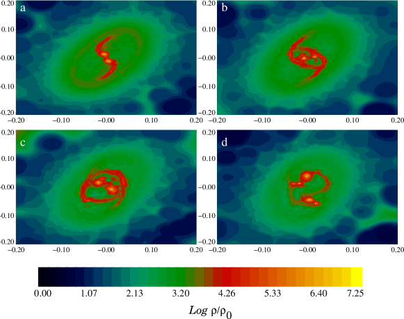
Figure 5: Iso-density plot for model m1b0045.

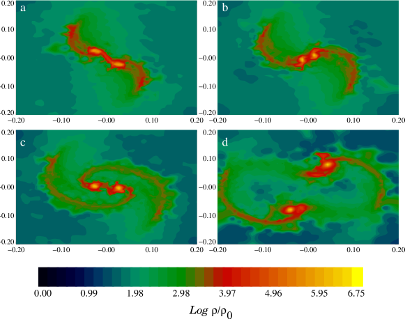
Figure 6: Iso-density plot for model m1b014.

3.2 Models with parent core mass $M_{0}=1.5\,M_{\odot}$

For the first time we saw that the low $\beta$ model m1p5b0045 did not produce a binary via the separation of its embryonic mass condensations, and instead we saw their merging. So, only a primary mass condensation is formed in the central core region, which is surrounded by small spiral arms, as can be seen in Fig.7. Soon thereafter, these spiral arms break and separate from the primary, so the simulation ended with a primary mass accompanied by two smaller mass condensations.

According to our strategy, we then increased the angular velocity of this model up to the value where we got $\beta=0.11$, so that we had now the model m1p5b011, in which we again obtained the appearance of a binary system via the separation of the embryonic mass condensations; see Fig.8. The binary separation in this case, 527 AU, is similar to that already seen in Section3.1 for the low $\beta$ model m1b014. The masses of the fragments for this new model are $0.16\,M_{\odot}$ and $0.17\,M_{\odot}$.

The existence of model m1p5b011 tells us in advance that the high $\beta$ model will form the desired binary, as can be seen in Fig.9, where we show the results for model m1p5b014. As was previously observed, the additional rotational energy produced a small increase in the binary separation, as we now obtained 585 AU, while the masses of the fragments were almost identical at $0.16\,M_{\odot}$.

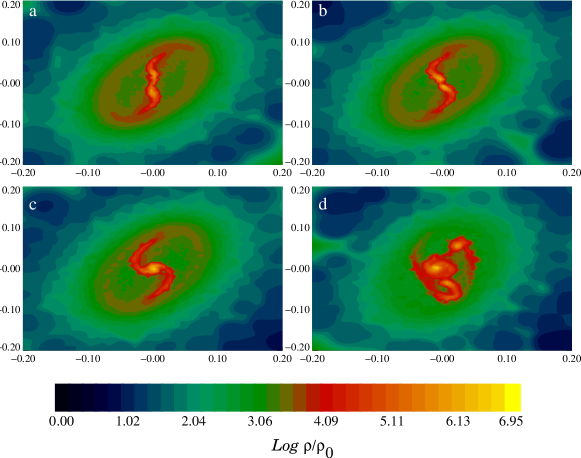
Figure 7: Iso-density plot for model m1p5b0045.

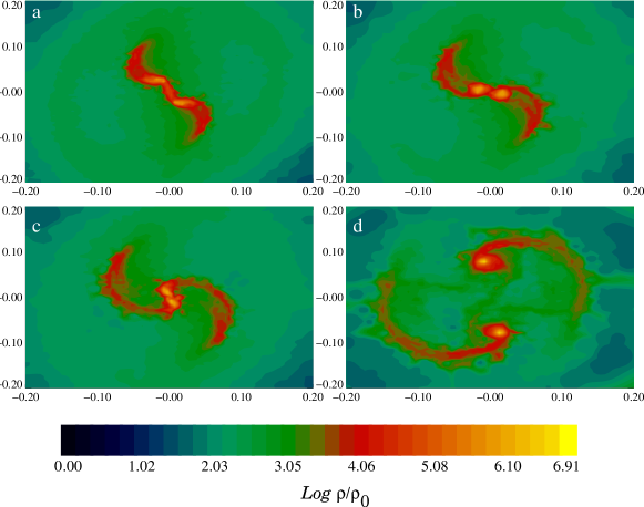
Figure 8: Iso-density plot for model m1p5b011.

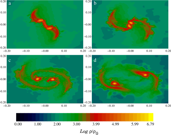
Figure 9: Iso-density plot for model m1p5b014.

3.3 Models with parent core mass $M_{0}=2.5\,M_{\odot}$

As was the case in Section 3.2, here the low $\beta$ model m2p5b0045 produced a primary configuration, which is shown in Fig.10. However, the high $\beta$ model m2p5b014 produce the desired binary configuration. For this reason, we expected to find a new $\beta$ value, such that the model m2p5b0045 would become a binary system. So, by systematically increasing its $\beta$, we reached the value $\beta=0.13$, where we found the desired configuration; see Fig.11. The results for model m2p5b014 are shown in Fig.12.

One would expect to find very similar physical properties for these pair of models, m2p5b013 and m2p5b014, as their initial $\beta$ values are very similar. The binary separations are indeed very similar, around 259 and 262 AU, respectively. However, the masses of their fragments are not so similar. This mass difference can be explained by closely looking Fig.11, where one can notice that there is an important mass exchange between the mass condensations, as the additional rotational energy supplied is perhaps barely enough to separate them, so they do not become true fragments.

3.4 Models with parent core mass $M_{0}=5\,M_{\odot}$

In this case we observed for the first time that even the high $\beta$ model does not produce the desired binary configuration. But we can still compare models m5b0045 and m5b014, as they form two slightly different primary dominated configurations. In model m5b0045, an elongated central bar is formed with two additional mass condensations formed at the ends of the spiral arms, as illustrated in Fig.13. In model m5b014 we see again the formation of a central mass condensation, but in this case, it is surrounded by very long spiral arms, which break soon thereafter and separate from this central mass; see Fig.14.

As usual, we then increased the level of the initial rotational energy, until the value of $\beta=0.21$, where we obtained the desired binary configuration, labeled now as model m5b021; see Fig.15. The binary separation is 427 AU while the masses of the fragments are $0.6\,M_{\odot}$ and $0.4\,M_{\odot}$.

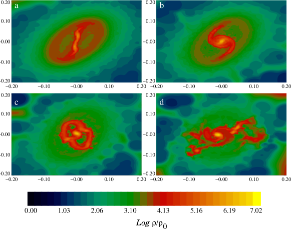
Figure 10: Iso-density plot for model m2p5b045.

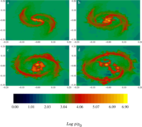
Figure 11: Iso-density plot for model m2p5b013.

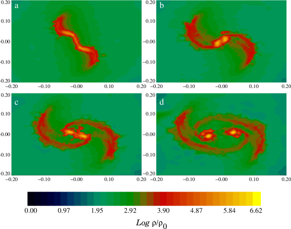
Figure 12: Iso-density plot for model m2p5b014.

4 Discussion

Table 2: Physical properties of fragments.

Model	$r_{max}/R_{0}$	$M_{f}/M_{\odot}$	$\alpha_{f}$	$\beta_{f}$
m075b0045	0.0125	1.2286294e-01	0.266161	0.181729
m075b0045	0.0125	3.2744151e-02	0.207690	0.261402
m075b014	0.0125	7.3241010e-02	0.202020	0.244268
m075b014	0.0125	7.0384055e-02	0.204878	0.237756
m1b0045	0.0164	1.6832440e-01	0.233851	0.265091
m1b0045	0.0164	9.3557134e-02	0.276662	0.213533
m1b014	0.0188	1.1661998e-01	0.207951	0.225678
m1b014	0.0188	1.1168584e-01	0.207141	0.243163
m1p5b011	0.028	1.6871537e-01	0.255228	0.171645
m1p5b011	0.028	1.7556763e-01	0.244072	0.195569
m1p5b014	0.028	1.6674188e-01	0.234014	0.243616
m1p5b014	0.028	1.6345865e-01	0.221192	0.234322
m2p5b013	0.0188	3.7504950e-01	0.239499	0.196338
m2p5b013	0.0188	1.0161296e-01	0.256503	0.124867
m2p5b014	0.0188	2.7242526e-01	0.246773	0.222628
m2p5b014	0.0188	2.6820856e-01	0.242448	0.205314
m5b021	0.0329	6.3345021e-01	0.249588	0.174287
m5b021	0.0329	4.0061280e-01	0.262765	0.159544

Table 3: Binary separation and the sound speed.

Model	$r_{sep}[AU]$	$c_{0}$ [cm/s]
m075b0045	111.43	13760.78
m075b014	402.98	13799.62
m1b0045	326.7	16647.83
m1b014	666.79	16647.83
m1p5b011	527.92	20000.0
m1p5b014	585.93	19711.58
m2p5b013	259	25410.62
m2p5b014	262.2	25410.62
m5b021	427.97	35820.06

The main results of this paper are already contained in Tables 1, 2 and 3. However, it is more illustrative to present them visually, so in Figs.16, 17, 18 and 19, we show: (i) the schematic diagram where the desired binary configurations are located; (ii) the obtained binary mass $M_{f}$ as a function of the total mass of the core $M_{0}$; (iii) the obtained binary separations and (iv) the distribution of the velocity field. Let us now comment upon the creation of each figure and their main results.

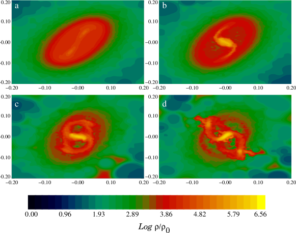
Figure 13: Iso-density plot for modelm5b045.

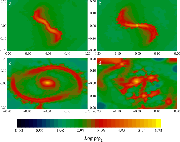
Figure 14: Iso-density plot for model m5b014.

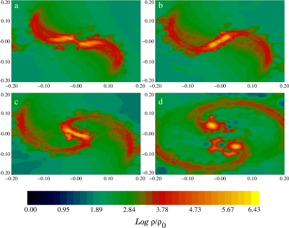
Figure 15: Iso-density plot for model m5b021.

4.1 The schematic diagram of binary configurations

The calculated schematic diagram of desired binary configurations is illustrated in Fig.16. We first notice that there must exist a critical mass $M_{crit}$ that corresponds to a $\beta_{crit}$, such that they separate two regimes: one where $M_{0}>M_{crit}$, in which the needed $\beta$ to obtain the desired binary configuration must be higher than the $\beta_{crit}$, but smaller than the maximum $\beta_{max}$ that allows to the core to remain in a bounded configuration, that is, $\beta$ is within the interval $\beta\,\in\,(\beta_{crit},\beta_{max})$.

Another regime, with $M_{0}<M_{crit}$, in which the needed $\beta$ can take values in the interval $0<\beta<\beta_{crit}$, where one can definitely obtain the desired binary configuration. However, there is still the possibility of having a binary configuration with even higher values of $\beta\,\in\,(\beta_{crit},\beta_{max})$, as the high value $\beta=0.14$ is set arbitrarily.

The cores were observed to have low rotational velocities, so if we had a collapsing core with $M_{0}<M_{crit}$, then according to Fig.16, it would be more likely to have a binary configuration resulting from its collapse. On the contrary, if we had a collapsing core with $M_{0}>M_{crit}$, then it would be more likely to have a primary system as the result of its collapse.

Figure 16: Schematic diagram to show the location of the binary systems. The mass $M_{0}$ is given in terms of $M_{\odot}$.

Figure 17: Binary mass given in terms of $M_{\odot}$.

4.2 The physical properties of binaries

Let us now consider Fig.17, recalling first that, as an approximation strategy to construct our simulation models, in this paper we increased the core mass $M_{0}$ without changing the core radius $R_{0}$, so the core density is increased and therefore the free fall time is decreased; see Eq.1.

The accreting mass rate can be inaccurately estimated by means of $\dot{M}=M_{0}/t_{ff}$; that is, as if the entire core mass had collapsed in a free fall time. The combinations of changes mentioned above, that the $M_{0}$ increases while the $t_{ff}$ decreases, gives us an increasing $\dot{M}$ for all the models under consideration.

A better estimate for the accreting mass rate was obtained by a semi-analytical approach to the collapse of an isothermal core; see [Shu et al. 1987], which is given now by $\dot{M}=c_{0}^{3}/G$, where $c_{0}$ is the sound speed and $G$ is Newton’s gravitational constant. In order to keep the ratio of thermal energy to gravitational energy, denoted by $\alpha$, fixed in all our models, we increased the sound speed in our models, so that one sees that the $\dot{M}$ increases when the mass of the core increases at least for the first stage of evolution where the isothermal approximation is valid.

So, the increase of the mass of the binary fragment with increase of the mass of the parent core is expected, as the mass accretion rate also increases with the mass of the parent core. In this paper we confirmed this expectation and we measured the binary mass $M_{f}$ obtained out of a given initial $M_{0}$. It should be noted that this fragment mass $M_{f}$ was determined in the following way: first we took the highest density particle in the region where the fragment was located. This particle is considered the center of the fragment. We then found all the SPH particles whose density was greater than or equal to some minimum density value given in advance by $\log_{10}\left(\rho_{min}/\rho_{0}\right)=5.0$ and that were within a given maximum radius $r_{max}$ from the fragment center; see the second column of Table 2. These parameters correspond to a minimum density of $3.82\,\times 10^{-13}\,$g cm^-3 and a maximum radius in the range of $r_{max}=41-100$ AU.

This set of particles defined the fragment and allowed us to calculate its integral properties; for instance, its mass $M_{f}$, and their ratios $\alpha_{f}$ and $\beta_{f}$. These calculated integral properties are shown in columns 3, 4 and 5 of Table 2, respectively, in which the number of selected particles falls in the range of 150 to 300 thousand, approximately.

In Section 3, we mentioned the calculated mass of the binary configurations. It is still necessary to comment on the calculated energy ratios $\alpha_{f}$ and $\beta_{f}$. It was demonstrated by [Arreaga et al. 2012] that in general the fragments obtained out by the fragmentation of a rotating core tend to virialize. We observed that for the last snapshot available in each simulation the sum of $\alpha_{f}$ and $\beta_{f}$ was always less than 0.5, so the fragments were still collapsing.

Finally, in order to determine the binary separations illustrated in Fig.18, we simply calculate the distance between the centers associated with each fragment, as defined according to the procedure outlined in the previous paragraph. It is important to mention that the longest binary separations were obtained for intermediate mass models: the m1b014 and m1p5b011; see Table 3.

Figure 18: Binary separation given in AU.

4.3 The velocity distribution of binaries

Now we shall discuss the velocity scale of the particles forming the fragments; see Fig.19. These plots are 3D representations formed by all the particles satisfying the following selection criteria: (i) they are located within the central region of the core, such that their projected radius $r_{2d}=\sqrt{x^{2}+y^{2}}$ is $r_{2d}<r_{2dmax}\equiv 0.2\,R_{0}$, irrespective of their $z$ coordinate; (ii) they have a density higher or equal than the minimum density value given in advance by $\log_{10}\left(\rho_{2dmin}/\rho_{0}\right)=4.0$. These parameters correspond to a minimum density $\rho_{2dmin}=3.82\,\times\,10^{-14}\,$g cm^-3 and a maximum radius of $r_{2dmax}=668$ AU. This selection procedure is similar to the one we used earlier to define a fragment. So, in this section, more particles were considered to make the 3D plots: in the range of 500-800 thousand, approximately.

We wish to point out that models have different sound speeds, $c_{0}$, which are shown in column three of Table 3. However, of this, in Fig.19 we plot the magnitude of the velocity vector, normalized with the sound speed, so that we will now use a Mach $\equiv v/c_{0}$, as the unit of velocity to describe our results.

In all the models, we observed that: (i) only very few particles reach very high velocities, marked with red color in the plots; it should be noted that these ultra-fast particles are located very close to the central region of the fragment and are velocity-isolated, as no other neighboring particles have similar velocities; (ii) particles located exactly in the center of the fragment have the smallest velocity, which can even range from 0.01 to 0.1 Mach, marked with blue color in the plots; (iii) spiral arms are connected to their fragments by particles with small velocities, marked with soft blue or aqua color in the plots; although not all of them are visible in these 3D plots, as their density is probably not high enough to satisfy our density selection criteria; (iv) the particles surrounding the innermost region of the fragments have intermediate velocities, marked with green color in the plots. These are the already rained particles from the spiral arms on the fragment. The particles that are still raining get the fragment through contact regions between the spiral arms and the fragments, where the raining particles have radial speeds it is marked with yellow color in the plots; (v) the co-existence of different color scales in a fragment indicates that there is a strong velocity gradient.

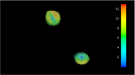
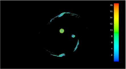
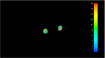
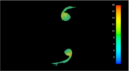
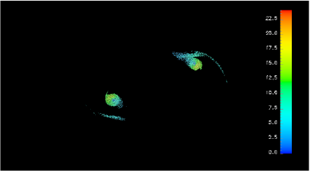
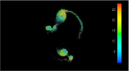
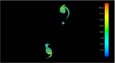
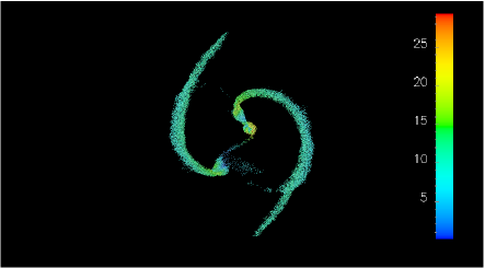
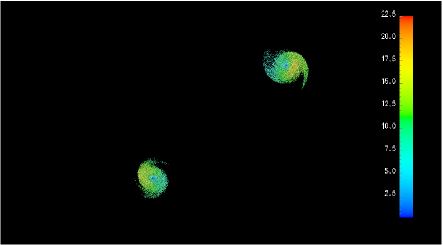
Figure 19: Iso-velocity 3D plot; each model is normalized with its corresponding sound speed, ordered from top to bottom according to the mass of the parent core: m5b021 (first line right); m2p5b013 (second line left), m2p5b014 (second line right); m1p5b011 (third line left), m1p5b014 (third line right); m1b045 (fourth line left), m1b014 (fourth line right) and m0p75b045 (fifth line left), m075b014 (fifth line right).

5 Concluding Remarks

In this paper we have considered the gravitational collapse of a rotating core using a spherical shell populated with SPH particles in order to represent the core at the initial simulation time.

First, we observed that this mesh geometry appropriately represents the relevant initial physics of the core, including the uniform density distribution and the rigid body rotation. There is an excess in density in early simulation time, as can be seen in Fig.2, which is likely to be a consequence of the huge surface density of the innermost radial shell. Fortunately, the particles quickly adjust themselves and thus the core truly begins its collapse some time later.

Second, the approximation strategy followed in this paper, that of changing the core mass while keeping the core radius unchanged, can be replaced by another, equally valid strategy, for instance, one in which both the core mass and the radius are changed while the average core density is unchanged. Hence, in this paper we can discuss certain results obtained for a family of similar size cores with slightly increasing total mass, while for the latter case one could discuss about of a family of similar density cores with slight mass and size variations.

Third, we observed that the more massive the initial core, the lower its tendency to obtain the desired binary system formed via the separation of the embryonic mass condensations. We thus prevented their merging by providing more initial rotational energy to the core. From the schematic configuration space reported in Fig.16, we conclude that it is more likely to have a binary system formed out of a small mass parent core and therefore the mass of the binaries are expected to be small as well.

Fourth, in order to calculate the integral properties and the velocity distributions of the obtained fragments, we took particles by applying selection criteria based on two parameters $lrho_{min}$ and $r{max}$ whose values were fixed in advance. The selected particles were those that had a density greater than or equal to $\rho_{0}\,\times 10^{lrho_{min}}$ and a position radius $r<r_{max}$. Thus, one would expect slight differences in the reported results as they are definition-dependent.

Nevertheless, we find that there is a clear correlation between the mass of the obtained fragments and the mass of the initial collapsing core. In fact, the masses of the fragments are within the observational range reported by [Tobin at al. 2013].

References

- [Arreaga et al. 2007] Arreaga-Garcia, G., Klapp, J., Sigalotti, L.G., & Gabbasov, R. 2007, ApJ, 666, 290-308.
- [Arreaga et al. 2008] Arreaga-Garcia, G., Saucedo, J., Duarte, R., & Carmona, J. 2008, Rev. Mex. Astron. Astrophys, 44, 259-284.
- [Arreaga & Klapp 2010] Arreaga-Garcia, G., & Klapp, J. 2010, A&A, 509, A96.
- [Arreaga et al. 2012] Arreaga-Garcia, G. , Saucedo, J., 2012, Rev. Mex. Astron. Astrophys, 48, Num. 1,61-84.
- [Balsara 1995] Balsara, D. 1995, J. Comput. Phys., 121, 357.
- [Bate & Burkert 1997] Bate, M.R., & Burkert, A., 1997, MNRAS, 288, 1060.
- [Bergin & Tafalla 2007] Bergin, E., & Tafalla, M. 2007, Annu. Rev. Astro. Astrophys., 45, 339
- [Boden 2011] Bodenheimer, P., Principles of star formation, Springer-Verlag, 2011.
- [Bodenheimer et al. 2000] Bodenheimer, P., Burkert, A., Klein, R.I., & Boss, A.P., in Protostars and Planets IV, Eds. V.G. Mannings, A.P. Boss & S.S. Russell, University of Arizona Press, Tucson, AZ, USA.
- [Boss 1991] Boss, A.P., 1991, Nature, 351, 298.
- [Boss et al. 2000] Boss, A.P., Fisher, R.T., Klein, R., & McKee, C.F. 2000, ApJ, 528, 325.
- [Boss & Bodenheimer 1979] Boss, A. P., & Bodenheimer, P. 1979, ApJ, 234, 289
- [Burkert & Alves 2009] Burkert, A., & Alves, J. (2009), ApJ, 695, 1308.
- [Burkert & Bodenheimer 1993] Burkert, A., & Bodenheimer, P. 1993, MNRAS, 264, 798
- [Duchêne et al 2004] Duchêne, G., Bouvier, J., Bontemps, S., André, P., & Motte, F. 2004, A&A, 427, 651.
- [Girart et al 2004] Girart, J. M., Curiel, S., Rodríguez, L. F., Honda, M., Cantó, J., Okamoto, Y. K., & Sako, S. 2004, AJ, 127, 2969.
- [Hachisu & Heriguchi 1984] Hachisu, I. and Heriguchi, Y., 1984, A&A,140,259.
- [Hachisu & Heriguchi 1985] Hachisu, I. and Heriguchi, Y., 1985, A&A,143,355.
- [Hennebelle et al 2004] Hennebelle, P., Whitworth, A. P., Cha, S.-H., & Goodwin, S. P. 2004, MNRAS, 348, 687.
- [Kitsionas & Whitworth 2002] Kitsionas, S., & Whitworth, A. P. 2002, MNRAS, 330, 129
- [Klein et al 1999] Klein, R. I., Fisher, R. T., McKee, C. F., & Truelove, J. K. 1999, in Numerical Astrophysics 1998, ed. S. Miyama, K. Tomisaka, & T. Hanawa (Dordrecht: Kluwer), 131.
- [Lucy & Ricco 1979] Lucy L.B., Ricco E., 1979, AJ 84, 401.
- [Matsumoto & Hanawa 2003] Matsumoto, T., & Hanawa, T. 2003, ApJ, 595, 913.
- [Miyama et al 1984] Miyama, S.M., Hayashi, C. and Narita, S., 1984, ApJ, 279, 621.
- [Monaghan & Gingold 1983] Monaghan, J.J., & Gingold, R.A. 1983, J. Comput. Phys., 52, 374
- [Myers 1983] Myers, P. C., Fragmentation of Molecular Cores and Star Formation, ed. E. Falgarone, F. Boulanger, & G. Duvert (Dordrecht, Kluwer), 1983, pp.221.
- [Reipurth et al 2002] Reipurth, B., Rodríguez, L. F., Anglada, G., & Bally, J. 2002, AJ, 124,1045.
- [Sigalotti & Klapp 2001] Sigalotti, L.G., & Klapp, J. 2001, International Journal of Modern Physics D, 10, 115.
- [Springel 2005] Springel, V. 2005, MNRAS, 364, 1105.
- [Shu et al. 1987] Shu, F.H., Adams, F.C. and Lizano, S. 1987, Annu. Rev. Astro. Astrophys, 25, pp.23-81.
- [Stahler & Palla 2004] Stahler, S.W. and Palla, F., The formation of stars, Wiley-Vch, 2004.
- [Sterzik et al. 2003] Sterzik, M.F., Durisen, R.H. and Zinnecker, H., ASTRONOMY & ASTROPHYSICS, 411, Num. 2, 2003, pp: 91-97.
- [Tobin et al. 2012] Tobin, J.J, Hartmann, L. & Chiang, H.F., 2012, Nature , 492, 83.
- [Tobin at al. 2013] Tobin, J.J, Chandler, C., Wilner, D.J., Looney, L.W.,Loinard, L., Chiang, H-F., Hartmann, L., Calvet, N., D’Alessio, P., Bourke, T.L. & Kwon, W.. 2013, ApJ, 779, Issue 2.
- [Tohline 2002] Tohline, J.E., 2002, Annu. Rev. Astro. Astrophys, 40, pp.349-385.
- [Tokovin 2000] Tokovinin, A.A., 2000, Astron. Astrophys. 360, 997.
- [Truelove et al. 1997] Truelove, J.K., Klein, R.I., McKee, C.F., Holliman, J.H., Howell, L.H., & Greenough, J.A., 1997, ApJ, 489, L179.
- [Truelove et al 1998] Truelove, J. K., Klein, R. I., McKee, C. F., Holliman, J. H., Howell, L. H., Greenough, J. A., & Woods, D. T. 1998, ApJ, 495, 821.
- [Tsuribe et al. 1999] Tsuribe, T. & Inutsuka, S-I., 1999, ApJ, 523, pp.L155-L158. Tsuribe, T. & Inutsuka, S-I., 1999, ApJ, 526, pp.307-313.
- [Tsuribe 2002] Tsuribe, T., 2002, PROGRESS OF THEORETICAL PHYSICS SUPPLEMENT , 147, pp.155-180. Tsuribe, T. & Inutsuka, S-I., 1999, ApJ, 526, pp.307-313.