Perturbation theory for the Fokker-Planck operator in chaos

Abstract

The stationary distribution of a fully chaotic system typically exhibits a fractal structure, which dramatically changes if the dynamical equations are even slightly modified. Perturbative techniques are not expected to work in this situation. In contrast, the presence of additive noise smooths out the stationary distribution, and perturbation theory becomes applicable. We show that a perturbation expansion for the Fokker-Planck evolution operator yields surprisingly accurate estimates of long-time averages in an otherwise unlikely scenario.

1 Introduction

The divergence of perturbation series due to small denominators in the vicinity of unstable fixed points, observed by Poincaré [1], was historically among the first hints of chaotic dynamics. This is enough to tell us that perturbative analysis might not get along with chaos.

Nonetheless, there have been successful attempts to treat instabilities with perturbation techniques, the first tracing back to Shimizu [2, 3, 4]. Shimizu model systems have a parameter which gradually drives them from periodicity to the onset of chaos. In that context, fast and slow time scales in the periodic phase allow for closed-form, asymptotic solutions, which shed light on the transition to chaos.

The validity of perturbation theory for systems far from equilibrium is intimately related to the existence of a linear response to the perturbation [5], an issue that has sparked great interest and some controversy [6, 7, 8] over the years. For maps in particular, we know that all smooth hyperbolic [9] and some partially hyperbolic diffeomorphisms [10] admit a linear response. The question is instead still open for a variety of physically interesting models, including the Hénon family, as well as piecewise hyperbolic maps [11, 12].

The object of our investigation is systems already deep in the fully chaotic regime, where in general one cannot separate time scales. We wish to determine whether the dynamics ever lends itself to a perturbative approach. The issue was notably addressed more than $20$ years ago by Ershov [13] in the context of one-dimensional maps, with the result that a perturbation of $O(\epsilon)$ to the original map would bring about a deviation up to $O(\epsilon\log\epsilon)$ in the response (see ref. [14] for a proof). Chaos breaks the proportionality between control parameter and statistical characteristics, disrupting the very basis of perturbation theory. Shortly later Ershov [15] established that the Perron-Frobenius operator becomes continuous in the presence of additive, uncorrelated noise. The response to perturbations of a density is then restored to $O(\epsilon)$, allowing in principle for perturbative calculations.

Proportionality between parameters and observables plays a major role in chaotic time series analysis [16], as first pointed out in ref. [17], where perturbations may be fruitfully used to test the robustness of the model [18]. In particular, dealing with long time series often boils down to building a Markov chain from the data. This can be expressed as a discretization of the Perron-Frobenius operator of the dynamics [19], whose leading eigenfunction, or invariant density, is used for the estimation of long time averages [20].

We organize the paper as follows: the Fokker-Planck evolution operator for a discrete-time dynamical system is introduced in sect. 2. In sect. 3 we add a small deterministic correction to a weakly noisy map, and develop a perturbation technique to approximate the corresponding Fokker-Planck operator. Our goal is to accurately estimate observables such as the escape rate from a noisy attractor, by using the stationary distribution (or invariant density, for a closed system) of the unperturbed noisy system. Direct numerical simulations of the weakly-noisy Lozi map with a small correction are compared to the perturbative approach in sect. 4. Our main result is that the perturbative estimates are in a close agreement with the outcomes of direct numerical simulations for a range of perturbations about an order of magnitude larger than expected. That constitutes quantitative evidence that the noise restores structural stability of the system, with the response proportional to the noise amplitude. Conclusions and comments are given in sect. 5.

2 The Fokker-Planck operator

The problem that we are considering involves adding a random variable to a map in $d$ dimensions that would otherwise exhibit deterministic chaos (the subscript $n$ represents time iteration):

$$x_{n+1}=f(x_{n})+\xi_{n}$$ (1)

The random variables $\xi_{n}$ are uncorrelated in time, independent, and distributed according to a Gaussian with a $[d\!\times\!d]$ covariance matrix

$$\Delta(x_{n})_{ij}=\langle\xi_{n}^{(i)}\xi_{n}^{(j)}\rangle\ \delta_{ij}\,,$$ (2)

which we allow to vary in position $x_{n}$ but not in time. Time is referenced by $n$. $i$ and $j$ range from 1 to $d$. Here we shall consider the evolution of densities of trajectories, according to the Fokker-Planck picture [21]. In discrete time, a distribution moves one time step according to the operator [22, 23]

$$\phi_{n+1}(y) = {\cal L}\phi_{n}\ (y)=\int\phi_{n}(x)\ \exp\left\{-\frac{1}{2}{[y-f(x)]}{}^{\top}\Delta^{-1}(x)[y-f(x)]\right\}\ [dx]$$ (3)

$${[dx]} = \frac{d^{d}\!x}{|\det(2\pi\Delta(x))|^{1/2}}\,.$$

The best information we can get about the long time behavior of the system is statistical. Recalling that we are interested in perturbations of steady states, the expectation value of any observable $a(x)$ can be found by knowing the escape rate $\gamma$ and stationary distribution $\rho(x)$

$$\langle a\rangle=\int e^{\gamma}\ \rho(x)\ a(x)\ dx.$$ (4)

The escape rate and the stationary distribution are respectively the logarithm of the maximal modulus (leading) eigenvalue and the leading eigenfunction of the Fokker-Planck operator,

$${\cal L}\ \rho(x)=e^{-\gamma}\rho(x).$$ (5)

As ${\cal L}$ is a non-negative operator, its leading eigenvalue is non-degenerate, real, and positive, and the corresponding eigenvector has non-negative coordinates, by Perron-Frobenius theorem [24, 25]. This property is also relevant for the applicability of perturbation theory.

The Fokker-Planck operator and its adjoint

$${\cal L}^{\dagger}\phi_{n}\ (y)=\int\phi_{n}(x)\ \exp\left\{-\frac{1}{2}{[x-f(y)]}{}^{\top}\Delta^{-1}(y)[x-f(y)]\right\}\ [dx]\$$ (6)

have a whole spectrum of distinct right and left eigenfunctions, which contain information on how an initial density decays to the stationary distribution,

$${\cal L}\ \rho_{i}(x)=\Gamma_{i}\ \rho_{i}(x)\hskip 20.00003pt{\cal L}^{\dagger}\ \tilde{\rho}_{i}(x)=\Gamma_{i}^{*}\ \tilde{\rho}_{i}(x).$$ (7)

Importantly, Eq. (3) defines an integral operator with a $L_{2}(R^{d})$ kernel (said of the Hilbert-Schmidt class [26]), and as such, it is bounded and thus continuous on its support, that is $\|\rho_{\epsilon}~{}-~{}\rho\|~{}\rightarrow~{}0$ implies $\|{\cal L}\rho_{\epsilon}-{\cal L}\rho\|\rightarrow 0$ and vice versa. As mentioned in the introduction, that is the main difference with the noiseless Perron-Frobenius operator, and the condition for us to apply perturbation theory (details are given in B).

3 Perturbation theory

Add a perturbation to the deterministic part of the system:

$$x_{n+1}=f^{(0)}(x_{n})+f^{(1)}(x_{n})+\xi_{n}.$$ (8)

The perturbation $f^{(1)}$ is small in a sense defined later. Without the noise, the new problem would be just as difficult as the original. The stationary distribution of a typical chaotic system has fractal structure; any finite perturbation results in the bifurcation of some of the infinitely many periodic orbits. The escape rate and other observables would thus change discontinuously. Perturbation theory would fail, in general. Here we have noise, and Eq. (8) results in a perturbation of the kernel of the original Fokker-Planck operator, which we only keep the first order of:

$$\exp\left\{-\frac{1}{2}[y-f^{(0)}(x)-f^{(1)}(x)]^{\top}\Delta^{-1}[y-f^{(0)}(x)-f^{(1)}(x)]\right\}\approx$$

$$\left(1\ +\ [y-f^{(0)}(x)]^{\top}\Delta^{-1}f^{(1)}(x)\right)\exp\left\{-\frac{1}{2}[y-f^{(0)}(x)]^{\top}\Delta^{-1}[y-f^{(0)}(x)]\right\}.$$ (9)

In order that the perturbation be small, we should have

$$\left|[y-f^{(0)}(x)]^{\top}\Delta^{-1}f^{(1)}(x)\right|\ll 1.$$ (10)

Suppose that the typical scale of the dynamics in the state space is $L$, so $|y-f^{(0)}(x)|\lesssim L$, and the amplitude of the noise in any direction is $\langle\xi_{n}^{(i)}\xi_{n}^{(i)}\rangle=2D$. We are considering weak noise with $(2D)^{1/2}\ll L$. The perturbation can be considered small if

$$|f^{(1)}(x)|\ll\frac{2D}{L}$$ (11)

everywhere on the attractor. We thus have three distinct length scales. The length scale associated with the unperturbed dynamics is much longer than the length scale associated with the noise. Both are much longer than the length scale associated with the perturbation to the dynamics.

Now that we have a first order perturbation to the operator, we can find the corresponding perturbations to the escape multiplier and stationary distribution. In the light of the observations made in the previous section on the properties of the leading eigenvalue/function of ${\cal L}$, we assume in what follows the $i^{th}$ eigenvalue of the unperturbed Fokker-Planck operator to be simple and non-splitting (that is, no phase transitions occur) under perturbations. Then, we perturb the eigenvalue problem and obtain

$$\big{(}{\cal L}^{(0)}+{\cal L}^{(1)}\big{)}\big{(}\rho^{(0)}_{i}+\rho^{(1)}_{i}\big{)}=\big{(}\Gamma^{(0)}_{i}+\Gamma^{(1)}_{i}\big{)}\big{(}\rho^{(0)}_{i}+\rho^{(1)}_{i}\big{)}.$$ (12)

Although this looks similar to the perturbation theory used in quantum mechanics, there are several complications. The Fokker-Planck operator is not self-adjoint, and thus right (left) eigenfunctions do not form an orthogonal set by themselves, but rather, right and left eigenfunctions form a bi-orthogonal set, namely $\int dx\tilde{\rho}_{i}(x)\rho_{i}(x)\neq 0$ only if $i=j$.

We also have a different normalization condition. Since the leading eigenfunction is a probability distribution, it is normalized according to $\int\rho(x)\ dx=1$. The normalization used in quantum perturbation theory is instead $\int\psi^{*}(x)\ \psi(x)\ dx=1$.

Take (12), keep only the first order terms, and cancel the unperturbed eigenvalue equation.

$${\cal L}^{(1)}\rho_{i}^{(0)}+{\cal L}^{(0)}\rho_{i}^{(1)}=\Gamma_{i}^{(1)}\rho_{i}^{(0)}+\Gamma_{i}^{(0)}\rho_{i}^{(1)}$$ (13)

To find the first order correction to the eigenvalue, multiply by the corresponding unperturbed left eigenfunction and integrate over the entire space.

$$\int\tilde{\rho}_{i}^{(0)}(x)^{*}{\cal L}^{(1)}\rho_{i}^{(0)}(x)\ dx\ +\ \int\tilde{\rho}_{i}^{(0)}(x)^{*}{\cal L}^{(0)}\rho_{i}^{(1)}(x)\ dx\ =\ \Gamma_{i}^{(1)}\int\tilde{\rho}_{i}^{(0)}(x)^{*}\rho_{i}^{(0)}(x)\ dx\ +\ \Gamma_{i}^{(0)}\int\tilde{\rho}_{i}^{(0)}(x)^{*}\rho_{i}^{(1)}(x)\ dx$$

$$\int\tilde{\rho}_{i}^{(0)}{\cal L}^{(1)}\rho_{i}^{(0)}+\int\tilde{\rho}_{i}^{(0)}{\cal L}^{(0)}\rho_{i}^{(1)}=\Gamma_{i}^{(1)}\int\tilde{\rho}_{i}^{(0)}\rho_{i}^{(0)}+\Gamma_{i}^{(0)}\int\tilde{\rho}_{i}^{(0)}\rho_{i}^{(1)}$$ (14)

$$\Longrightarrow\int\tilde{\rho}_{i}^{(0)}{\cal L}^{(1)}\rho_{i}^{(0)}=\Gamma_{i}^{(1)}\ \int\tilde{\rho}_{i}^{(0)}\rho_{i}^{(0)}.$$ (15)

The first order correction to the eigenvalue is thus:

$$\Gamma_{i}^{(1)}=\frac{\int\tilde{\rho}_{i}^{(0)}{\cal L}^{(1)}\rho_{i}^{(0)}}{\int\tilde{\rho}_{i}^{(0)}\rho_{i}^{(0)}}.$$ (16)

We recall that the theory presented so far applies to a non-negative operator of the Hilbert-Schmidt class, thus infinite dimensional. In order to find the first order correction to the eigenfunction, rewrite (13) so that each side looks like an eigenvalue equation.

$$\left({\cal L}^{(0)}-\Gamma_{i}^{(0)}{\bf 1}\right)\rho_{i}^{(1)}=-\left({\cal L}^{(1)}-\Gamma_{i}^{(1)}{\bf 1}\right)\rho_{i}^{(0)}$$ (17)

To isolate $\rho_{i}^{(1)}$, we would like to invert $\left({\cal L}^{(0)}-\Gamma_{i}^{(0)}{\bf 1}\right)$. Unfortunately, this is guaranteed to not be invertible since $\Gamma_{i}^{(0)}$ is an eigenvalue of ${\cal L}^{(0)}$. If the Fokker-Planck operator were self-adjoint like in quantum mechanics, the eigenfunctions would form a complete basis, and the perturbation to the eigenfunction could be written as a superposition of the unperturbed eigenfunctions, except the one that we are calculating the perturbation to. The orthogonality of the eigenfunctions would then allow us to isolate the coefficients of the first order correction of the eigenfunction in this basis of unperturbed eigenfunctions (see for example [27]). But since ${\cal L}^{(0)}$ is neither Hermitian nor in general diagonalizable, we may not proceed in this fashion, and instead we get around the problem by using the Moore-Penrose pseudoinverse [28], $\left({\cal L}^{(0)}-\Gamma_{i}^{(0)}{\bf 1}\right)^{+}$, that first projects the subspace of $\Gamma_{i}^{(0)}$ out of ${\cal L}^{(0)}~{}-~{}\Gamma_{i}^{(0)}~{}{\bf 1}$, and then takes the inverse of the resulting operator. In order to evaluate this pseudoinverse, we have to introduce some truncated basis for $L_{2}(R^{d})$, and thus restrict our analysis henceforth to a finite-dimensional subspace. The operator equation (18) is then reduced to a matrix equation which can be solved numerically. The details of this procedure are shown in C. At the end, we obtain

$$\rho_{i}^{(1)}=-\left({\cal L}^{(0)}-\Gamma_{i}^{(0)}{\bf 1}\right)^{+}{\cal L}^{(1)}\rho_{i}^{(0)}.$$ (18)

Note that the normalization of the unperturbed eigenfunction is irrelevant. Multiplying the unperturbed eigenfunction by a constant simply multiplies the perturbation by the same constant, so the relative size of the perturbation remains unchanged.

The properties of the Moore-Penrose operator and its relation to other pseudoinverses are reported in D.

4 Numerical results for the Lozi map

We test this technique on the Lozi map with a deterministic correction $q(x,y)$, and weak, white noise:

$$x_{n+1} = 1-a\ |x_{n}|+b\ y_{n}+\epsilon\ q(x_{n},y_{n})+\xi_{n}^{(x)}$$

$$y_{n+1} = x_{n}+\xi_{n}^{(y)}$$ (19)

The random variable added to this system is uniformly distributed according to

$$P(\xi)=\frac{1}{\sqrt{\det{(2\pi\Delta)}}}\exp{\Big{(}-\frac{1}{2}{\xi}{}^{\top}\Delta^{-1}\xi\Big{)}}.$$ (20)

Here $\Delta$ is isotropic. Its magnitude varies over the course of this study.

The Lozi map is a two-dimensional version of the tent map [figure 1(a)], and it undergoes a bifurcation cascade as the slope (controlled by the parameter $a$) is varied (figure 2). Here we set $a=1.85$ and $b=0.3$, corresponding to chaotic dynamics confined in the attractor of figure 1(b).

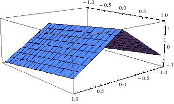
(a) (b)

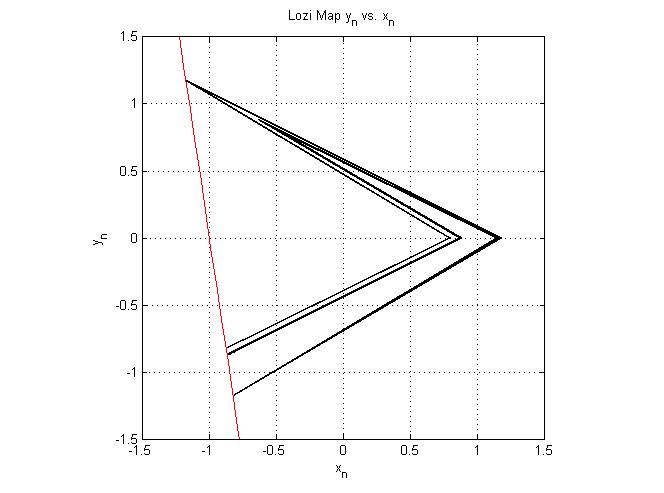
Figure 1: (a) $f(x,y)=1-a|x|+by$ shows the ‘tent’ shape of the Lozi map, its slope controlled by the parameter $a$; (b) the Lozi attractor with parameters $a=1.85,b=0.3$ calculated using the long time behavior of a single generic orbit. The red line shows the boundary of the basin of attraction. Any points to the left of that line escape to $(-\infty,-\infty)$ and any points to the right approach the attractor as the map is iterated without noise.

The additive perturbation $q(x,y)$ is a smooth function, while $\epsilon$ is the small parameter and can be either positive or negative. In what follows, we will take $q(x,y)=x^{2}$ (analyses of the cases $q(x,y)=x^{3}$ and $q(x,y)=y^{2}$ can be found in A), which is of particular interest, being qualitatively equivalent to a perturbation of the parameter $a$, where the bifurcations are understood. So, for example, when $\epsilon>0$, adding $\epsilon x^{2}$ to the Lozi map is equivalent to decreasing the parameter $a$ and thus slightly deforming the attractor of figure 1(b) [or figure 2(e)], whereas $\epsilon<0$ effectively increases the parameter $a$, so as to turn the Lozi attractor of figure 2(e) into a repeller [figure 2(f)].

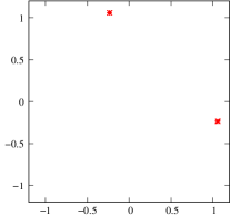
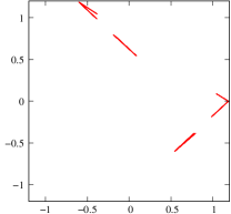
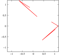
(a) (b) (c) (d) (e) (f)

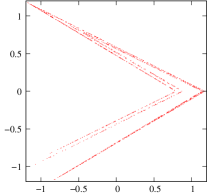
Figure 2: Snapshots of the bifurcation cascade of the Lozi map, from (a) a period-2 stable cycle for $a=1$, to: (b) a period-4 stable cycle ($a=1.3$); (c) a four-region chaotic attractor ($a=1.35$); (d) a two-region chaotic attractor ($a=1.4$); (e) the one-region attractor used in this study ($a=1.85$), that quickly fades into a repeller when the parameter is further increased, as in (f) ($a=1.855$).

We divide the region ${\cal M}=[-1.5,1.5]\times[-1.5,1.5]$ into 3600 uniform grid elements, and we call each ${\cal M}_{k}$. When calculating the perturbation to the eigenfunction, we use the basis of characteristic functions for each of our grid elements.

$$\chi_{k}(x)\equiv\left\{\begin{array}[]{cl}\frac{1}{\sqrt{|{\cal M}_{k}|}}&\mbox{if $x\in{\cal M}_{k}$}\\ 0&\mbox{otherwise .}\end{array}\right.$$ (21)

We want to compute the leading eigenvalue and eigenfunction from a numerical approximation of the one-step transfer matrix [29], that is the discretized Fokker-Planck operator, whose entries are probabilities of a trajectory to hop between any pair of grid elements in one time step. The transfer matrix is given by

$${\cal L}_{ij}=\int_{{\cal M}_{i}}[dy]\int_{{\cal M}_{j}}[dx]\exp\left\{-\frac{1}{2}{[y-f(x)]}{}^{\top}\Delta^{-1}(x)[y-f(x)]\right\}$$ (22)

that in general would be a $2N$-dimensional integral (4D in our model). Since the kernel of the operator is smooth, and it varies on a length scale longer than the grid mesh, as long as the amplitude of the noise in our simulations is large enough, we may approximate (22) with

$${\cal L}_{ij}\simeq\exp\left\{-\frac{1}{2}{[y_{j}-f(x_{i})]}{}^{\top}\Delta^{-1}[y_{j}-f(x_{i})]\right\},$$ (23)

where $x_{i}$ and $y_{j}$ are the centers of the corresponding grid elements. We may ensure the validity of the above approximation by estimating the error from the first-order Taylor expansion of the integrand in (22), and applying the mean value theorem for integrals, so that the ratio of the overall remainder of the integral to the leading term (23) is upper bounded by

$$|l^{2}|\sup_{{\cal M}_{i},{\cal M}_{j}}\left|\nabla^{2}\exp\left\{-\frac{1}{2}{[y-f(x)]}{}^{\top}\Delta^{-1}(x)[y-f(x)]\right\}\right|.$$ (24)

The size $l$ of the mesh in the discretization is $O(10^{-2})$, while $f(x)$ is (piecewise) linear and at most $O(1)$ on the Lozi attractor, hence (24) is $O(10^{-4})$ or less, orders of magnitude smaller than the typical size of the perturbation in Eq. (9).

The Lozi map is not globally attracting. The stable manifold of one of the two fixed points acts as a boundary for the basin of attraction (see figure 1). Without the noise, any orbit which begins in the basin of attraction will stay on the attractor for all time. The noise allows orbits to cross this boundary and results in a nonzero escape rate. Once an orbit crosses the deterministic boundary, it accelerates off to $(-\infty,-\infty)$. To account for this, we say that an initial condition escapes in one time step if it crosses the deterministic boundary of the basin of attraction. These points are excluded from the calculation of the transfer matrix (23). Once we have the transfer matrix, we calculate the eigenvalues and eigenvectors. The largest magnitude eigenvalue is the escape multiplier $\Gamma_{0}=e^{-\gamma}$, where $\gamma$ is the escape rate. Since our system is ergodic, the largest magnitude eigenvalue is guaranteed to be real and isolated [30].

Our goal is to estimate the escape rate, as well as the stationary distribution of (19) to the first non-trivial order of perturbation, according to (16) and (18), respectively. We utilize in these formulae the stationary distributions $\rho^{(0)}(x)$ and $\tilde{\rho}^{(0)}(x)$ of the unperturbed ($\epsilon=0$) Fokker-Planck operator ${\cal L}^{(0)}$ and its adjoint $\left[{\cal L}^{(0)}\right]^{\dagger}$, respectively, computed by means of (23). On the other hand, we apply the same discretization to diagonalize the transfer matrix of the perturbed map (19) ($\epsilon\neq 0$), as a way to check the accuracy of the perturbation theory calculation.

We perform our calculations for two different noise amplitudes, $\Delta=0.1\ {\bf 1}$ and $\Delta=0.01\ {\bf 1}$, to investigate how the strength of the noise influences the efficacy of perturbation theory, and we compute the escape rate for a range of values of the small parameter $\epsilon$, controlling the size of the deterministic perturbation. Based on Eq. (11), we can predict roughly that the perturbation theory will break down at $\epsilon\sim 2D/L\approx 0.05,0.005$, depending on the noise amplitude. Figure 3 illustrates the results: the escape rate computed with perturbation theory [(16)] is in agreement with the result from the diagonalization of the transfer matrix (22) for the full map (19), for a range of $\epsilon$ about an order of magnitude larger than what estimated with Eq. (11).

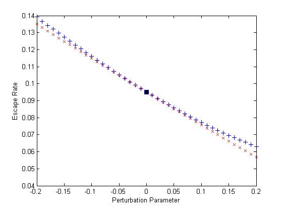
(a) (b)

Figure 3: The escape rate $\gamma$ from the Lozi attractor, as a function of the perturbation parameter $\epsilon$, for: (a) $\Delta=.1\ {\bf 1}$ and (b) $\Delta=.01\ {\bf 1}$. Blue pluses: exact calculation. Red crosses: perturbation theory.

Next, the stationary distribution $\rho^{(1)}(x)$ is computed to the first non-trivial perturbative order using (18), and then again compared with the first eigenfunction $\rho(x)$ of the spectrum of (23), by means of the $L_{2}$ distance

$$d({\rho},{\rho}^{(1)})=\frac{\int\left[{\rho}(x)-{\rho}^{(1)}(x)\right]^{2}dx}{\int\left[{\rho}(x)\right]^{2}dx}.$$ (25)

Density plots of the calculated distributions are shown in figure 4 and figure 5. Due to the small value of $\epsilon$, the stationary distributions ${\rho}(x),{\rho}^{(1)}(x)$ of the perturbed map can hardly be distinguished from the invariant density ${\rho}^{(0)}(x)$ of the unperturbed system. To make the distinctions more apparent, we also plot the differences

$$\delta{\rho}(x) = \frac{{\rho}(x)-{\rho}^{(0)}(x)}{\epsilon},$$ (26)

$$\delta{\rho}^{(1)}(x) = \frac{{\rho}^{(1)}(x)-{\rho}^{(0)}(x)}{\epsilon}.$$ (27)

As shown in the figures, the differences $\delta{\rho}(x)$ and $\delta{\rho}^{(1)}(x)$ look almost identical, as evidence that ${\rho}^{(1)}(x)$ is a good estimate for ${\rho}(x)$. The range of validity of the perturbative approximation for the stationary distribution is probed in figure 6, where the $L_{2}$ distances $d({\rho}^{(0)},{\rho})$, $d({\rho}^{(0)},{\rho}^{(1)})$, and $d({\rho}^{(1)},{\rho})$ are plotted as a function of $\epsilon$. It is apparent from the graph that $d({\rho}^{(0)},{\rho})\sim\epsilon^{2}$, and $d({\rho}^{(0)},{\rho}^{(1)})\sim\epsilon^{2}$, which is in agreement with the expectation $\|{\cal L}_{\epsilon}\rho-{\cal L}\rho\|\sim\epsilon$ (proven in B). Surprisingly, instead, the $L_{2}$ distance $d({\rho}^{(0)},{\rho}^{(1)})\ll\epsilon$ for a range of $|\epsilon|$ that largely exceeds the expectations.

(a)
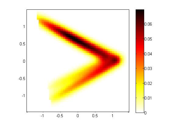
(b) (c)
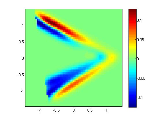
(d) (e)

Figure 4: Density plots of the stationary distributions for $\Delta=.01\ {\bf 1}$ and $\epsilon=.05$. (a) ${\rho}^{(0)}(x)$. (b) ${\rho}(x)$. (c) $\delta{\rho}(x)$. (d) ${\rho}^{(1)}(x)$. (e) $\delta{\rho}^{(1)}(x)$.

(a)
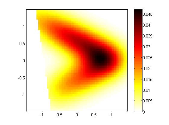
(b) (c)
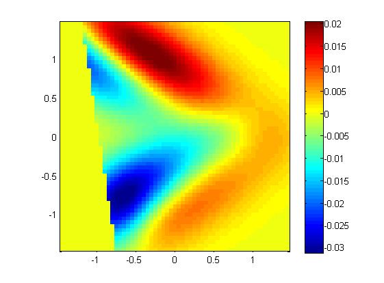
(d) (e)

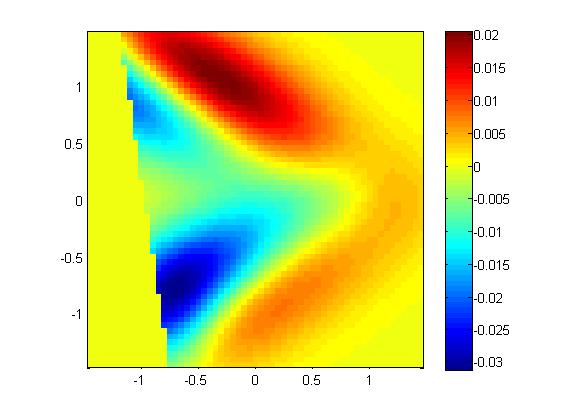
Figure 5: Density plots of the stationary distributions for $\Delta=.1\ {\bf 1}$ and $\epsilon=.05$. (a) ${\rho}^{(0)}(x)$. (b) ${\rho}(x)$. (c) $\delta{\rho}(x)$. (d) ${\rho}^{(1)}(x)$. (e) $\delta{\rho}^{(1)}(x)$.

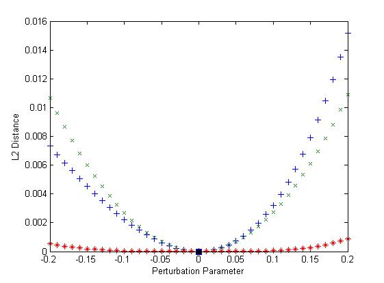
(a) (b)

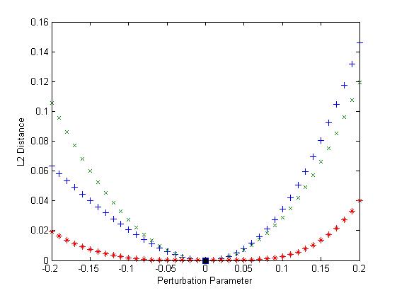
Figure 6: $L_{2}$ distance $d$ between various distributions as a function of the perturbation parameter $\epsilon$. Blue pluses: $d({\rho}^{(0)},{\rho})$. Green crosses: $d({\rho}^{(0)},{\rho}^{(1)})$. Red asterisks: $d({\rho}^{(1)},{\rho})$. (a) $\Delta=.1\ {\bf 1}$ and (b) $\Delta=.01\ {\bf 1}$.

5 Conclusions, comments

The fractal structure of the stationary distribution for a system exhibiting deterministic chaos changes discontinuously in response to any finite perturbation, in principle preventing any perturbative calculations.

In contrast, weak noise smears out these fractals. This is apparent in a Fokker-Planck picture: the evolution operator becomes continuous, the stationary distribution (natural measure) is smooth, and, consequently, the system lends itself to a perturbative treatment.

We have expanded the Fokker-Planck evolution operator of a noisy map subject to a deterministic perturbation in a power series. The long-time observables of the perturbed system can be estimated in terms of the unperturbed one. As an example, we have obtained excellent approximations to the escape rate and to the stationary distribution of a noisy Lozi attractor, valid for a range of the perturbation parameter proportional to the amplitude of the noise, and always at least one order of magnitude larger than expected.

The successful implemetation of perturbation theory in a chaotic system affected by weak noise can also be relevant for the following reasons:

1. the relative insensitivity to fluctuations demonstrated constitutes evidence that a chaotic system acquires a finite resolution when noise is introduced, and it can be modelled via a transfer operator of finite degrees of freedom. This problem is discussed extensively in [22, 23, 31];

2. the analysis presented sets bounds for the robustness of a model, and it is straightforward enough to be implemented in any algorithm that creates a template out of a time series. It is noted that low-dimensional, noisy discrete-time mappings are still widely used as models in several fields of science and engineering [32, 33, 34].

Future work in this direction may investigate

1. the validity of higher-order expansions, which we do not expect to change the results reported here qualitatively, at least for the leading eigenvalue/function of the Fokker-Planck operator. The reason is that perturbation series are trivial about simple, non-splitting eigenvalues, while one has fractional (‘Puiseux’ [26]) power series in the vicinity of phase transitions, with successive terms (much) less than an order of magnitude apart from one another;

2. evolution operators which carry finite memory of the past (for example of the Mori-Zwanzig type  [35, 36]), as opposed to the Markovian operators considered here, and whether and to what extent those lend themselves to a perturbative approach. Markovian operators other than the Fokker-Planck operator are implemented in the same way: just replace the Gaussian in (3) and (6) with a different kernel.

6 Acknowledgments

D.L. acknowledges the National Science Fundation of China (NSFC) for partial support (Grant No. 11450110057-041323001). J.M.H. thanks D.L. and Prof. Nianle Wu for the hospitality at IASTU, Beijing, where part of this work was done. P.C. thanks the family of late G. Robinson, Jr. and NSF grant DMS-1211827 for partial support.

Appendix A Additional perturbations

We present in this section the outcomes of additional tests of perturbation theory, with corrections of the forms $q(x,y)=x^{3}$ (figure 7) and $q(x,y)=y^{2}$ (figure 8) for the Lozi map.

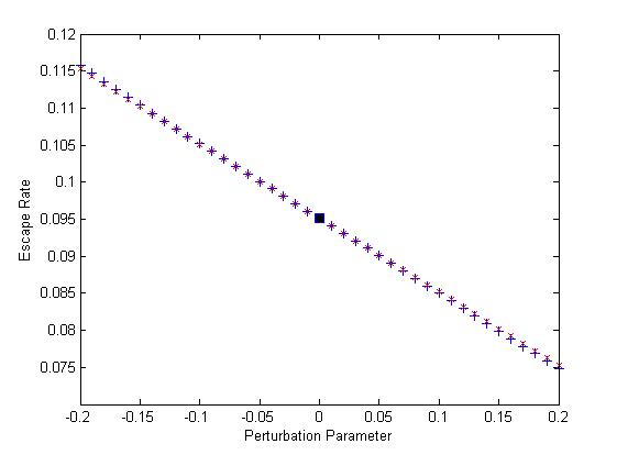
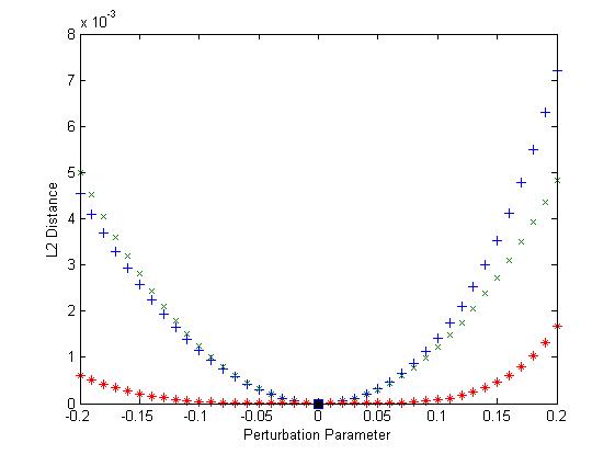
(a) (b)
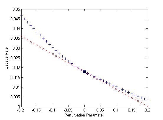
(c) (d)

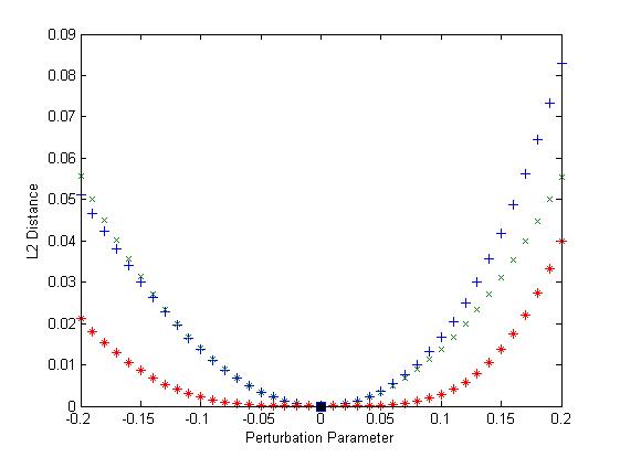
Figure 7: [(a),(b)] Escape rate $\gamma$ vs. perturbation parameter $\epsilon$ for a perturbation of the form $q(x,y)=x^{3}$. Blue pluses: exact calculation. Red crosses: perturbation theory. (a) $\Delta=.1{\bf 1}$ (b) $\Delta=.01{\bf 1}$. [(c),(d)] $L^{2}$ distance $d$ vs. $\epsilon$. Blue pluses: $d({\rho}^{(0)},{\rho})$. Green crosses: $d({\rho}^{(0)},{\rho}^{(1)})$. Red asterisks: $d({\rho}^{(1)},{\rho})$. (c) $\Delta=.1{\bf 1}$ (d) $\Delta=.01{\bf 1}$.

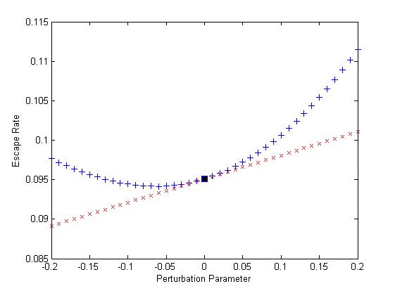
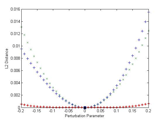
(a) (b)
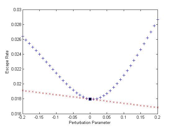
(c) (d)

Figure 8: [(a),(b)] Escape rate $\gamma$ vs. perturbation parameter $\epsilon$ for a perturbation of the form $q(x,y)=y^{2}$. Blue pluses: exact calculation. Red crosses: perturbation theory. (a) $\Delta=.1{\bf 1}$ (b) $\Delta=.01{\bf 1}$. [(c),(d)] $L^{2}$ distance $d$ vs. $\epsilon$. Blue pluses: $d({\rho}^{(0)},{\rho})$. Green crosses: $d({\rho}^{(0)},{\rho}^{(1)})$. Red asterisks: $d({\rho}^{(1)},{\rho})$. (c) $\Delta=.1{\bf 1}$ (d) $\Delta=.01{\bf 1}$.

Appendix B Continuity of the Fokker-Planck operator and response to perturbations

The Fokker-Planck operator ${\cal L}$, supported on a bounded interval $I$, defines a bounded mapping of $L_{2}(I)$ into itself. In fact, calling the kernel

$$L(x,y)=\frac{1}{|\det(2\pi\Delta(x))|^{1/2}}\exp\left\{-\frac{1}{2}{(y-f(x))}{}^{\top}\Delta^{-1}(x)(y-f(x))\right\},$$ (28)

we may write

$$\|{\cal L}\rho\|^{2} = \int\left|\int L(x,y)\rho(y)dy\right|^{2}dx$$ (29)

$$\leq \int\left(\int|L(x,y)|^{2}dy\right)\left(\int|\rho(y)|^{2}dy\right)dx=\|L\|^{2}\|\rho\|^{2}<\infty,$$

where $\rho$ is supposed $L_{2}$, and all integrals are taken on a compact interval. We want to show that a perturbation of $O(\epsilon)$ produces a response of the same order. That is

$$\|{\cal L}_{\epsilon}\rho-{\cal L}\rho\|\sim\epsilon,$$ (30)

where

$${\cal L}_{\epsilon}\rho=\int\rho(x)\ \exp\left\{-\frac{1}{2}{(y-f(x)-\epsilon f^{1}(x))}{}^{\top}\Delta^{-1}(x)(y-f(x)-\epsilon f^{1}(x))\right\}\ [dx].$$ (31)

The exponential form allows us to separate the kernel and recast the $\epsilon-$dependence into the distribution it acts on

$${\cal L}_{\epsilon}\rho={\cal L}\rho_{\epsilon},$$ (32)

and we may rewrite

$$\|{\cal L}_{\epsilon}\rho-{\cal L}\rho\| = \|{\cal L}\rho_{\epsilon}-{\cal L}\rho\|\leq\|L\|\,\|\rho_{\epsilon}-\rho\|$$ (33)

$$\simeq \|L\|\,\|[1-\epsilon yf^{1}(x)]\rho-\rho\|=\epsilon\|L\|\,\|yf^{1}(x)\rho\|,$$

that is of $O(\epsilon)$, as required.

Appendix C First order corrections in terms of a particular basis

Choose a basis to represent everything in: $\{H_{k}\}$, where

$$\int H_{j}\ H_{k}\ dx=\delta_{jk}.$$

Note that this is not the same normalization that is used to make the leading eigenvector a probability distribution. This means that the coefficients of the distributions in this representation have units, but leads to no other negative side effects.

Write both the perturbed and unperturbed eigenfunctions in this basis.

$$\rho_{i}^{(0)}(x) = \sum_{k}P^{(0)}_{ik}\ H_{k}(x)$$ (34)

$$\rho_{i}^{(1)}(x) = \sum_{k}P^{(1)}_{ik}\ H_{k}(x)$$ (35)

We will also need to have the unperturbed adjoint eigenfunction using the same basis.

$$\tilde{\rho}_{i}^{(0)}(x)=\sum_{k}\tilde{P}^{(0)}_{ik}\ H_{k}(x)$$ (36)

The unperturbed Fokker-Planck operator or perturbation to the Fokker-Planck can be written using a kernel.

$${\cal L}\ \rho_{i}(y)=\int L(y,x)\ \rho_{i}(x)\ dx$$ (37)

These kernels can also be written in terms of our basis.

$$L^{(0)}(y,x) = \sum_{jk}L^{(0)}_{jk}\ H_{j}(y)\ H_{k}(x)$$ (38)

$$L^{(1)}(y,x) = \sum_{jk}L^{(1)}_{jk}\ H_{j}(y)\ H_{k}(x)$$ (39)

The action of an operator acting on an eigenfunction in terms of the basis is:

$${\cal L}\ \rho_{i}(y) = \int L(y,x)\ \rho_{i}(x)\ dx$$ (40)

$$= \int\left(\sum_{jk}L_{jk}\ H_{j}(y)\ H_{k}(x)\right)\ \left(\sum_{l}P_{il}\ H_{l}(x)\right)\ dx$$ (41)

$$= \sum_{jkl}P_{il}\ L_{jk}\ H_{j}(y)\int H_{k}(x)\ H_{l}(x)\ dx$$ (42)

$$= \sum_{jk}P_{ik}\ L_{jk}\ H_{j}(y)$$ (43)

Start by writing the first order correction to the eigenvalue using this basis representation. The first order correction to the eigenvalue is given in (16).

$$\Gamma_{i}^{(1)} = \frac{\int\left(\sum_{l}\tilde{P}^{(0)}_{il}\ H_{l}(x)\right)\ \left(\sum_{jk}P^{(0)}_{ik}\ L^{(1)}_{jk}\ H_{j}(x)\right)\ dx}{\int\left(\sum_{j}\tilde{P}^{(0)}_{ij}\ H_{j}(x)\right)\ \left(\sum_{k}P^{(0)}_{ik}\ H_{k}(x)\right)\ dx}$$ (44)

$$= \frac{\sum_{jk}\tilde{P}^{(0)}_{ij}\ P^{(0)}_{ik}\ L^{(1)}_{jk}}{\sum_{j}\tilde{P}^{(0)}_{ij}\ P^{(0)}_{ij}}$$ (45)

Write this in matrix notation.

$$\Gamma_{i}^{(1)}=\frac{{\tilde{p}^{(0)}_{i}}{}^{\top}\ \mathbf{L}^{(1)}\ p^{(0)}_{i}}{{\tilde{p}^{(0)}_{i}}{}^{\top}\ p^{(0)}_{i}}$$ (46)

To find the first order correction to the eigenfunction, write (13) entirely in terms of this basis. We are interested in finding the coefficients $P^{(1)}_{ik}$.

$$\sum_{jk}P^{(1)}_{ik}\ L^{(0)}_{jk}\ H_{j}(x)+\sum_{mn}P^{(0)}_{in}\ L^{(1)}_{mn}\ H_{m}(x)=\Gamma^{(0)}_{i}\sum_{a}P^{(1)}_{ia}\ H_{a}(x)+\Gamma^{(1)}_{i}\sum_{b}P^{(0)}_{ib}\ H_{b}(x)$$ (47)

Multiply this by $H_{l}(x)$ and integrate over $x$ to get an expression relating only the coefficients.

$$\sum_{k}P^{(1)}_{ik}\ L^{(0)}_{lk}+\sum_{n}P^{(0)}_{in}\ L^{(1)}_{ln}=\Gamma^{(0)}_{i}\ P^{(1)}_{il}+\Gamma^{(1)}_{i}\ P^{(0)}_{il}$$ (48)

Rearrange this to make it look like eigenvalue equations. This will help us isolate $P^{(1)}_{il}$.

$$\sum_{k}\left(L^{(0)}_{lk}-\Gamma^{(0)}_{i}\delta_{lk}\right)\ P^{(1)}_{ik}=-\sum_{n}\left(L^{(1)}_{ln}-\Gamma^{(1)}_{i}\delta_{ln}\right)\ P^{(0)}_{in}$$ (49)

Rewrite this in matrix notation.

$$\left(\mathbf{L}^{(0)}-\Gamma^{(0)}_{i}{\bf 1}\right)p^{(1)}_{i}=-\left(\mathbf{L}^{(1)}-\Gamma^{(1)}_{i}{\bf 1}\right)p^{(0)}_{i}$$ (50)

The matrix $\mathbf{L}^{(0)}-\Gamma^{(0)}_{i}{\bf 1}$ is not invertible since $\Gamma^{(0)}_{i}$ is an eigenvalue of ${\cal L}^{(0)}$.

We can use the pseudoinverse, now applied to a matrix, to write an explicit expression for the coefficients of the first order correction to the eigenfunction.

$$p^{(1)}_{i}=-\left(\mathbf{L}^{(0)}-\Gamma^{(0)}_{i}{\bf 1}\right)^{+}\left(\mathbf{L}^{(1)}-\Gamma^{(1)}_{i}{\bf 1}\right)p^{(0)}_{i}.$$ (51)

Appendix D The Moore-Penrose and other pseudoinverses

In this section we state the properties of the Moore-Penrose pseudoinverse, the Drazin pseudoinverse, and the group inverse, and show that they all coincide for the operator ${\cal L}^{(0)}~{}-~{}\Gamma_{i}^{(0)}~{}{\bf 1}$, used in the text.

The Moore-Penrose pseudoinverse of a rectangular matrix $A$ has the following properties  [28]

$$AA^{+}A=A,$$ (52)

$$A^{+}AA^{+}=A^{+},$$ (53)

$$\left(AA^{+}\right)^{\dagger}=AA^{+},$$ (54)

$$\left(A^{+}A\right)^{\dagger}=A^{+}A.$$ (55)

This operator is of common use, due to its generality. A similar operation is performed by the Drazin (pseudo)inverse  [37], used for example by Kato  [26], who calls it reduced resolvent (denoted as ${\cal L}^{(0)}~{}-~{}\Gamma_{i}^{(0)}~{}{\bf 1}$,  [38]) of the unperturbed operator ${\cal L}^{(0)}$. The Drazin inverse is defined for a square matrix $A$ in an associative ring (or a semigroup), and it has the following properties:

$$A^{k+1}A^{\#}=A^{k},$$ (56)

$$A^{\#}AA^{\#}=A^{\#},$$ (57)

$$AA^{\#}A=A,$$ (58)

$$AA^{\#}=A^{\#}A.$$ (59)

Here $k=ind(A)$ is the index of $A$, that is the smallest nonnegative integer such that $rank(A^{k})=rank(A^{k+1})$. The index also coincides with the multiplicity of the eigenvalue $0$, or equivalently, the dimension of the kernel of the matrix  [39]. Importantly, Drazin and Moore-Penrose operators coincide and are called group inverse if $ind(A)=~{}1$  [40]. That is the case of the operator ${\cal L}^{(0)}~{}-~{}\Gamma_{i}^{(0)}~{}{\bf 1}$, whose kernel is one-dimensional since the eigenvalue $\Gamma_{i}^{(0)}$ of ${\cal L}^{(0)}$ is simple.

For completeness, we include the properties of the group inverse  [41, 42]

$$AA^{g}A=A$$ (60)

$$A^{g}AA^{g}=A^{g}$$ (61)

$$AA^{g}=A^{g}A.$$ (62)

References

References

- Poincaré [1899] Poincaré, H.. Les Méthodes Nouvelles de la Méchanique Céleste. Paris: Guthier-Villars; 1899. For a very readable exposition of Poincaré’s work and the development of the dynamical systems theory up to 1920’s see ref. [43].
- Shimizu [1987a] Shimizu, T.. Perturbation theory analysis of chaos I. Physica A 1987a;142:75–102.
- Shimizu [1987b] Shimizu, T.. Perturbation theory analysis of chaos II. Physica A 1987b;145:341–360.
- Shimizu [1991] Shimizu, T.. Perturbation theory analysis of chaos III. Physica A 1991;178:101–122.
- Kubo [1957] Kubo, K.. Statistical mechanical theory of irreversible processes. I. J Phys Soc Japan 1957;12:570–586.
- van Kampen [1971] van Kampen, N.G.. Case against linear response theory. Phys Norv 1971;5:279.
- Saito and Matsunaga [1989] Saito, N., Matsunaga, Y.. Linear response theory formulated from the chaotic dynamics. J Phys Soc Japan 1989;58:3089–3105.
- Suhl [1994] Suhl, H.. Chaos and the Kubo formula. Physica B 1994;199/200:1–7.
- Ruelle [1997] Ruelle, D.. Differentiation of SRB states. Commun Math Phys 1997;187:227.
- Dolgopyat [2004] Dolgopyat, D.. On differentiability of SRB states for partially hyperbolic systems. Invent Math 2004;155:389.
- Ruelle [2009] Ruelle, D.. A review of linear response theory for general differentiable dynamical systems. Nonlinearity 2009;22:855–870. 0901.0484.
- Baladi [2014] Baladi, V.. Linear response, or else. In: Jang, S.Y., Kim, Y.R., Lee, D.W., Yie, I., editors. Proceedings of the International Congress of Mathematicians. Seoul, South Korea: Kyung Moon Sa Co. Ltd.; 2014, p. 525–545. 1408.2937.
- Ershov [1993] Ershov, S.V.. Is a perturbation theory for dynamical chaos possible? Phys Lett A 1993;177:180–185.
- Keller et al. [2008] Keller, G., Howard, P.J., Klages, R.. Continuity properties of transport coefficients in simple maps. Nonlinearity 2008;21:1719–1743. doi:10.1088/0951-7715/21/8/003.
- Ershov [1994] Ershov, S.V.. Even the first iterate of a Markov operator is contracting in an norm. J Stat Phys 1994;74:783–813.
- Durbin and Koopman [2012] Durbin, J., Koopman, S.J.. Time series analysis by state space methods. Oxford: Oxford Univ. Press; 2012.
- Tang et al. [1995] Tang, X.Z., Tracy, E.R., Boozer, A.D., deBrauw, A., Brown, R.. Symbol sequence statistics in noisy chaotic signal reconstruction. Phys Rev E 1995;51:3871–3889.
- Maybhate and Amritkar [2000] Maybhate, A., Amritkar, R.E.. Dynamic algorithm for parameter estimation and its applications. Phys Rev E 2000;61(6):6461–6470.
- Froyland [2001] Froyland, G.. Extracting dynamical behaviour via Markov models. In: Mees, A., editor. Nonlinear Dynamics and Statistics: Proc. Newton Institute, Cambridge 1998. Boston: Birkhäuser. ISBN 978-1-4612-6648-8; 2001, p. 281–321. doi:10.1007/978-1-4612-0177-9_12.
- Cvitanović et al. [2016] Cvitanović, P., Artuso, R., Mainieri, R., Tanner, G., Vattay, G.. Chaos: Classical and Quantum. Copenhagen: Niels Bohr Institute; 2016. URL: http://ChaosBook.org/.
- Risken [1996] Risken, H.. The Fokker-Planck Equation. New York: Springer; 1996. ISBN 978-3-540-61530-9.
- Lippolis and Cvitanović [2010] Lippolis, D., Cvitanović, P.. How well can one resolve the state space of a chaotic map? Phys Rev Lett 2010;104:014101. doi:10.1103/PhysRevLett.104.014101; 0902.4269.
- Cvitanović and Lippolis [2012] Cvitanović, P., Lippolis, D.. Knowing when to stop: How noise frees us from determinism. In: Robnik, M., Romanovski, V.G., editors. Let’s Face Chaos through Nonlinear Dynamics. Melville, NY: American Institute of Physics; 2012, p. 82–126. doi:10.1063/1.4745574; 1206.5506.
- Walters [1981] Walters, P.. An Introduction to Ergodic Theory. New York: Springer; 1981.
- Ruelle [1968] Ruelle, D.. Statistical mechanics of a one-dimensional lattice gas. Commun Math Phys 1968;9:267–278.
- Kato [1980] Kato, T.. Perturbation Theory for Linear Operators. Berlin: Springer; 1980. ISBN 9783662126783.
- Sakurai [1994] Sakurai, J.J.. Modern Quantum Mechanics. Reading, Mass.: Addison-Wesley-Longman; 1994.
- Barata and Hussein [2012] Barata, J.C.A., Hussein, M.S.. The Moore-Penrose pseudoinverse. A tutorial review of the theory. Braz J Phys 2012;42:146–165. 1110.6882.
- Ulam [1960] Ulam, S.M.. A Collection of Mathematical Problems. New York: Interscience; 1960.
- Ruelle [1978] Ruelle, D.. Statistical Mechanics, Thermodynamic Formalism. Reading, MA: Addison-Wesley; 1978.
- Heninger et al. [2015] Heninger, J.M., Lippolis, D., Cvitanović, P.. Neighborhoods of periodic orbits and the stationary distribution of a noisy chaotic system. Phys Rev E 2015;92:062922. doi:10.1103/PhysRevE.92.062922; 1507.00462.
- Ray et al. [2009] Ray, W., Rogers, J.L., Wiesenfeld, K.. Coherence between two coupled lasers from a dynamics perspective. Opt Expr 2009;17:9357–68. doi:10.1364/OE.17.009357.
- Beirami et al. [2012] Beirami, A., Nejati, H., Ali, W.H.. Zigzag map: a variability-aware discrete-time chaotic-map truly random number generator. Electron Lett 2012;48:1537–1538. doi:10.1049/el.2012.2762.
- Quail et al. [2015] Quail, T., Shrier, A., Glass, L.. Predicting the onset of period-doubling bifurcations in noisy cardiac systems. Proc Natl Acad Sci USA 2015;112:9358–9363.
- Chorin et al. [2002] Chorin, A., Hald, O., Kupferman, R.. Optimal prediction with memory. Physica D 2002;166:239–257.
- Venturi and Karniadakis [2014] Venturi, D., Karniadakis, G.E.. Convolutionless Nakajima-Zwanzig equations for stochastic analysis in nonlinear dynamical systems. Proc R Soc A 2014;470:20130754. doi:10.1098/rspa.2013.0754.
- Drazin [1958] Drazin, M.P.. Pseudo-inverses in associative rings and semigroups. Am Math Monthly 1958;65:506–514. doi:10.2307/2308576.
- Avrachenkov et al. [2013] Avrachenkov, K.E., Filar, J.A., Howlett, P.G.. Analytic Perturbation Theory and Its Applications. Philadelphia: SIAM; 2013. doi:10.1137/1.9781611973143.
- Agaev and Chebotarev [2002] Agaev, R.P., Chebotarev, P.Y.. On determining the eigenprojection and components of a matrix. Automation and Remote Control 2002;63:1537–1545.
- Bu et al. [2012] Bu, C., Feng, C., Dong, P.. A note on computational formulas for the Drazin inverse of certain block matrices. J Appl Math Comput 2012;38:631–640. doi:10.1007/s12190-011-0501-4.
- Ben-Israel and Greville [1974] Ben-Israel, A., Greville, T.N.E.. Generalized Inverses: Theory and Applications. New York: Wiley; 1974.
- Campbell and Meyer [1979] Campbell, S.L., Meyer, C.D.. Generalized Inverses of Linear Transformations. London: Pitman; 1979.
- Barrow-Green [1997] Barrow-Green, J.. Poincaré and the Three Body Problem. Providence R.I.: Amer. Math. Soc.; 1997.