Numerical calculation of scaling exponents of percolation process in the framework of renormalization group approach

Abstract

We use the renormalization group theory to study the directed bond percolation (Gribov process) near its second-order phase transition between absorbing and active state. We present a numerical calculation of the renormalization group functions in the $\epsilon$-expansion where $\epsilon$ is a deviation from the upper critical dimension $d_{c}=4$. Within this procedure anomalous dimensions $\gamma$ are expressed in terms of irreducible renormalized Feynman diagrams and thus the calculation of renormalization constants could be entirely skipped. The renormalization group is included by means of the $R$ operation, and for computational purposes we choose the null momentum subtraction scheme.

1 Introduction

The renormalization group (RG) method is a theoretical framework which is especially suitable for studying various critical phenomena Vasiliev ; Amit . From a computational point of view it provides techniques for a perturbative calculation of different critical exponents. One of the most prominent dynamical models Tauber2014 which exhibits a second order phase transition is the directed bond percolation Stauffer ; HHL08 . In the physical literature it is known also as Schlögl first reaction Schlogl . Among others it explains hadron interactions at very high energies (Reggeon field theory) Cardy , stochastic reaction-diffusion processes on a lattice Hinrichsen , spreading of infection diseases Janssen , etc. The critical exponents are calculable in the form of perturbative expansion in a formally small parameter $\epsilon$. We note that two-loop results for the exponents $z$ and $\delta$ were obtained in Bronzan and exponents $\nu$ and $\beta$ later on in Janssen81 . All necessary information concerning percolation process in terms of reaction-diffusion model can be found in the review article Janssen .

As is in detail discussed in the literature Vasiliev (Part 3.5) or Amit (Part 7.5) the central idea behind renormalization group is freedom in choose of particular renormalization scheme. All of them makes a theory finite with respect to ultraviolet divergences and regarding universal quantities they lead to the same result. For practical numerical calculations it is more convenient to choose the subtractions at normalization point $\{p=0,\omega=0,\tau=\mu^{2}\}$ as explained in Vasiliev (see Eq. (3.18)).

Furthermore, in the renormalized Green function it is possible to replace an additional contribution of the renormalized constant by the operator $R$ Vasiliev applied to Green functions

$$\Gamma^{R}=R\Gamma=(1-K)R^{\prime}\Gamma,$$ (1)

where $R^{\prime}$ is the incomplete operator $R$ that cancels divergences in subgraphs of a given graph and the operator $(1-K)$ eliminates the remaining superficial divergence.

The main of this work is to show main steps of alghoritmic procedure, which allows us to reproduce known two-loops results to very high precision. Moreover it easy to generalize our procedure to high orders and thus obtaine more reliable results.

2 Renormalization of the model

A field theoretical formulation of the percolation process Janssen is based on the following action

$$S=\psi^{\dagger}(-\partial_{t}+D_{0}\partial^{2}-D_{0}\tau_{0})\psi+\frac{D_{0}\lambda_{0}}{2}[(\psi^{\dagger})^{2}\psi-\psi^{\dagger}\psi^{2}],$$ (2)

where $\psi$ is a coarse-grain density of percolating agents, $\psi^{\dagger}$ is an auxiliary (Martin-Siggia-Rose) response field, $D_{0}$ is a diffusion constant, $\lambda_{0}$ is a positive coupling constant and $\tau_{0}$ is a deviation from the threshold value of injected probability (an analog of critical temperature in static models). The model is studied near its critical dimension $\epsilon=4-d$ in the region where $\tau_{0}$ acquires its critical value. The expansion parameter of the perturbation theory is rather $\lambda_{0}^{2}$ than $\lambda_{0}$ as it could be easily seen by a direct inspection of Feynman diagrams. Hence it is more convenient to introduce a new charge $u=\lambda^{2}$. The renormalized action functional can be written in the following form

$$S_{R}=\psi^{\dagger}(-Z_{1}\partial_{t}+Z_{2}D\partial^{2}-Z_{3}D\tau)\psi+\frac{Z_{4}D\lambda\mu^{\epsilon}}{2}[(\psi^{\dagger})^{2}\psi-\psi^{\dagger}\psi^{2}].$$ (3)

It can be shown Janssen that this kind of a model is multiplicatively renormalizable. Furthermore the action functional $S_{R}$ can also be obtained from the action $S$ by the standard procedure of multiplicative renormalization of all the fields and parameters

$$\psi_{0}=\psi Z_{\psi},\hskip 14.22636pt\psi_{0}^{\dagger}=\psi^{\dagger}Z_{\psi^{\dagger}},\hskip 14.22636ptD_{0}=DZ_{D},\hskip 14.22636pt\lambda_{0}=\lambda\mu^{\epsilon}Z_{\lambda},\hskip 14.22636pt\tau_{0}=\tau Z_{\tau}.$$ (4)

The relations between renormalized constants $Z_{i},i=1,2,3,4$ are obtained in a straightforward fashion and read

$$Z_{1} =Z_{\psi}Z_{\psi^{\dagger}}, Z_{2} =Z_{D}Z_{\psi}Z_{\psi^{\dagger}},$$

$$Z_{3} =Z_{D}Z_{\tau}Z_{\psi}Z_{\psi^{\dagger}}, Z_{4} =Z_{D}Z_{\lambda}Z_{\psi^{\dagger}}^{2}Z_{\psi}=Z_{D}Z_{\lambda}Z_{\psi^{\dagger}}Z_{\psi}^{2}.$$ (5)

Moreover, the relation $Z_{\psi}=Z_{\psi^{\dagger}}$ is satisfied. In this work, at the normalization point (NP) $p=0$, $\omega=0$ and $\tau=\mu^{2}$ is considered. The counterterms are then specified at the normalization point (NP), and it is advantageous to express renormalization constants in terms of normalized Green functions

$$\bar{\Gamma}_{1}=\partial_{i\omega}\Gamma_{\psi^{\dagger}\psi}\big{|}_{p=0,\omega=0}, \bar{\Gamma}_{3} =-\frac{\Gamma_{\psi^{\dagger}\psi}-\Gamma_{\psi^{\dagger}\psi}\big{|}_{\tau=0}}{D\tau}\Big{|}_{p=0,\omega=0},$$

$$\bar{\Gamma}_{2}=-\frac{1}{2D}\partial_{p}^{2}\Gamma_{\psi^{\dagger}\psi}\big{|}_{p=0,\omega=0}, \bar{\Gamma}_{4} =\frac{\Gamma_{\psi^{\dagger}\psi^{\dagger}\psi}-\Gamma_{\psi^{\dagger}\psi\psi}}{D\lambda\mu^{\epsilon}}\Big{|}_{p=0,\omega=0},$$ (6)

that satisfy the following conditions $\bar{\Gamma}_{i}^{R}|_{\tau=\mu^{2}}=1,\quad i=1,2,3,4.$ RG constants defined by these conditions do not depend on $m$, like in minimal subtraction (MS) scheme. Accordingly RG equations are the same as in MS scheme

$$(\mu\partial_{\mu}+\beta_{u}\partial_{u}-\tau\gamma_{\tau}\partial_{\tau}-D\gamma_{D}\partial_{D})\Gamma_{i}^{R}=(n_{\psi}\gamma_{\psi}+n_{\psi^{\dagger}}\gamma_{\psi^{\dagger}})\Gamma_{i}^{R},$$ (7)

where $\mu$ is a reference mass scale, $n_{\psi}$ and $n_{\psi_{\dagger}}$ are the numbers of the corresponding fields entering the Green function under consideration, $\gamma_{x}=\mu\partial_{\mu}\log Z_{x}$ are anomalous dimensions and $\beta_{u}=u(-2\epsilon-\gamma_{u})$ is a beta function describing a flow of the charge $u$ under the RG transformation Vasiliev . Using these equations we find relations for the normalized functions

$$(\mu\partial_{\mu}+\beta_{u}\partial_{u}-\tau\gamma_{\tau}\partial_{\tau}-D\gamma_{D}\partial_{D})\bar{\Gamma}_{i}^{R}=\gamma_{i}\bar{\Gamma}_{i}^{R}.$$ (8)

Here, anomalous dimensions $\gamma_{i}$ are obtained from relations (5) between the renormalization constants

$$\gamma_{1}=2\gamma_{\psi},\quad\gamma_{3}=2\gamma_{\psi}+\gamma_{D}+\gamma_{\tau},\quad\gamma_{2}=2\gamma_{\psi}+\gamma_{D},\quad\gamma_{4}=3\gamma_{\psi}+\gamma_{D}+\gamma_{\lambda}.$$ (9)

Taking into account the renormalization scheme we can express the anomalous dimension in terms of the renormalized derivatives of the one-particle irreducible Green function $\bar{\Gamma}_{i}$ at the normalization point Adzhemyan2011 ; Adzhemyan2013 ; Adzhemyan2014

$$F_{i}\equiv-[\tilde{\tau}\partial_{\tilde{\tau}}\bar{\Gamma}_{i}^{R}(\tilde{\tau})]\big{|}_{\tilde{\tau}=1},\quad i=1,2,4$$ (10)

where $\tilde{\tau}={\tau}/{\mu^{2}}$. At the normalization point ($\tilde{\tau}=1$), $\gamma_{i}$ takes the form Adzhemyan2011 ; Adzhemyan2013

$$\gamma_{i}=\frac{2F_{i}}{1+F_{2}-F_{3}},\quad i=1,2,4.$$ (11)

For later considerations it is reasonable to introduce new functions (see Adzhemyan2013 )

$$f_{i}\equiv R[-\tilde{\tau}\partial_{\tilde{\tau}}\bar{\Gamma}_{i}(\tilde{\tau})]\big{|}_{\tilde{\tau}=1}.$$ (12)

These functions are related to the functions $F_{i}$ (10) in the following way

$$f_{i}-F_{i}=f_{i}F_{3},\hskip 28.45274pti=1,2,4.$$ (13)

We rewrite equations in (11) to obtain relations for anomalous dimensions in terms of the renormalized derivatives of the one-irreducible Green function $\bar{\Gamma}_{i}$ with respect to $\tilde{\tau}$ at the normalized point

$$\gamma_{i}=\frac{2f_{i}}{1+f_{2}},\quad i=1,2,4.$$ (14)

The main benefit of this procedure considering (12) is that the operator $R$ is taken at the normalization point and it can be expressed in terms of a subtracting operator $1-K_{i}$ that eliminates all divergences from the Feynman graphs Vasiliev

$$R\Gamma=\prod\limits_{i}(1-K_{i})\Gamma,$$ (15)

where the product is taken over all relevant subgraphs of the given Feynman graph, including also the graph as a whole. In the NM scheme we obtain the following representation for the $R$-operator Adzhemyan2011 ; Adzhemyan2014

$$R\chi=\prod\limits_{i}\frac{1}{n_{i}!}\int\limits_{0}^{1}da_{i}(1-a_{i})^{n_{i}}\partial^{n_{i}+1}_{a_{i}}\chi(\{a\}),$$ (16)

where the product is taken over all one-irreducible subgraphs $\chi_{i}$ (again including the graph $\chi$ as a whole) with the canonical dimension $n_{i}\geq 0$ and $a_{i}$ is a parameter that stretches momenta flowing into the $i$-th subgraph inside this graph. The main outcome of this approach is that integrals are finite for $\epsilon=0$. This scheme enables us to calculate a contribution from each diagram to counterterms Adzhemyan2011

$$Z_{i}=\frac{2}{n\epsilon}\left[f_{i}-J\bar{\Gamma}_{i}^{(n)}\right],$$ (17)

where $n$ is a number of loops. The second term on the RHS stands for a sum of diagrams of lower order perturbation theory. This allows us to recursively calculate counterterms in the NM scheme at the normalized point and thus gives us an opportunity to compare the results with ones obtained in the MS scheme.

3 Calculation of anomalous dimensions

In this part, we illustrate the method described in the previous section by its application to a specific diagram. Let us consider a two-loop contribution to $f_{3}$ from (12) determined by the two-loop three-point diagram of $\Gamma_{4}$

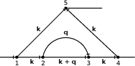
Figure 1: The two-loop Feynman diagram of $\Gamma_{4}$ with symmetry factor equal to one.

with the dimension $n_{\chi}=0$. The diagram has one relevant subgraph: the subgraph given by vertices $\{2,3\}$ with the dimension $n_{a}=2$.

The action of the differential operator $-\tilde{\tau}\partial_{\tilde{\tau}}$ on the line $G(k)=1/(k^{2}+\tilde{\tau})$ produces an additional factor $1/(k^{2}+\tilde{\tau})$ and it corresponds to the insertion of a unit vertex into the propagator line. Graphically it will be denoted by the additional two-point interaction vertex. The application of the operator to the diagram results into a sum over all possible insertions of the vertex

$$-\tilde{\tau}\partial_{\tilde{\tau}}\chi=\raisebox{-17.22217pt}{\epsfbox{graph_a}}+\raisebox{-17.22217pt}{\epsfbox{graph_b}}+\dots$$ (18)

The next step consists of the inclusion of the operator $R$, but the analysis of each diagram has to be made separately. For example for the first diagram on the RHS of Eq.(18), with the point outside the subgraph, nothing changes the dimension of the subgraph and $n_{a}=2$ remains valid. On the other hand, in the second graph, the subgraph becomes logarithmic and the corresponding dimension is changed to $n_{a}=0$. In this way we obtain the expansion

$$R\left(-\tilde{\tau}\partial_{\tilde{\tau}}\chi\right)\big{|}_{\tilde{\tau}=1}=\frac{1}{2}\int\limits_{0}^{1}da(1-a)^{2}\partial_{a}^{3}\raisebox{-17.22217pt}{\epsfbox{graph_a}}+\int\limits_{0}^{1}da\partial_{a}\raisebox{-17.22217pt}{\epsfbox{graph_b}}+\dots.$$ (19)

Further it is necessary to multiply all external parameters for a given subgraph by the parameter $a$. For the propatagor line this means that $G(q+k)=1/[(aq+k)^{2}+1]$.

Combining (9) and (12) we can derive relations for anomalous dimensions $\gamma$ for fields and parameters of the model

$$\gamma_{\psi}=\frac{f_{1}}{1+f_{2}}, \gamma_{D} =\frac{2(f_{2}-f_{1})}{1+f_{2}}, \gamma_{u} =2\frac{2f_{4}-f_{1}-2f_{2}}{1+f_{2}},$$ (20)

where $f_{i}$s are given up to the two-loop approximation by the following expressions:

$$f_{1}=-\frac{u}{16}+\frac{u\epsilon}{32}+0.0152772u^{2},\quad f_{2}=-\frac{u}{32}+\frac{u\epsilon}{64}+0.0062804u^{2},\quad f_{4}=-\frac{u}{4}+\frac{u\epsilon}{8}+0.117185u^{2}.$$ (21)

These results were obtained by a numerical calculation in which the actual form of integrals is determined by the $R$ operator using the Feynman representation. Subsequently, the momentum integrals are calculated by the Monte Carlo methods Cuba . To the second order of perturbation theory, there are $2$ diagrams for the function $\Gamma_{\psi^{\dagger}\psi}$ and $11$ diagrams for the function $\Gamma_{\psi^{\dagger}\psi^{2}}$.

The scaling regimes are associated with the fixed points (FPs) of the RG transformation. The asymptotic large scale behavior is governed by the infrared fixed points. Their coordinates can be found from the requirement that $\beta$-functions vanish. The directed bond percolation process has only one $\beta$-function

$$\beta_{u}=u(-2\epsilon-\gamma_{u})\approx u\left(-2\epsilon+\frac{3u}{4}-\frac{3u\epsilon}{8}-\frac{3u^{2}\epsilon}{128}-0.389626u^{2}\right).$$ (22)

There are two FPs given by the equation above: the trivial (Gaussian or free) FP ($u=0$) and the non-trivial one of the following form:

$$u^{*}=\frac{8}{3}\epsilon+5.02756\epsilon^{2}+O(\epsilon^{3}).$$ (23)

that corresponds to the critical percolation process. After the determination of the FP coordinates, critical exponents can be analyzed. First, the critical exponent $\eta$ takes the following value

$$\eta\equiv 2\gamma_{\psi}\big{|}_{u=u^{*}}=-\frac{\epsilon}{3}-0.27228\epsilon^{2}+O(\epsilon^{3}).$$ (24)

The second is the so-called dynamical exponent $z$ which is associated with the distinctive behavior with respect to the time direction

$$z\equiv 2-\gamma_{D}\big{|}_{u=u^{*}}=2-\frac{\epsilon}{6}-0.11682\epsilon^{2}+O(\epsilon^{3}).$$ (25)

Needed momentum integrals were calculated with the numerical precision of $10^{-4}$. For comparison with an analytic calculation we report the appropriately changed results (rescaling $\epsilon\rightarrow 2\epsilon$ is needed) from Janssen81 ; Janssen

$$\eta = -\frac{\epsilon}{3}\left[1+\left(\frac{25}{144}+\frac{161}{72}\textrm{ln}\frac{4}{3}\right)\epsilon+O(\epsilon^{2})\right]\approx-\frac{\epsilon}{3}-0.2723000633\epsilon^{2}+O(\epsilon^{3}),$$ (26)

$$z = 2-\frac{\epsilon}{6}\left[1+\left(\frac{67}{144}+\frac{59}{72}\textrm{ln}\frac{4}{3}\right)\epsilon+O(\epsilon^{2})\right]\approx 2-\frac{\epsilon}{6}-0.1168362090\epsilon^{2}+O(\epsilon^{3}).$$ (27)

We thus obtain excellent agreement with our results (24) and (25).

Our two-loop results are in agreement with analytic calculations and our numerical method is suitable for the calculation of the Feynman graphs to the three-loop order. To this end, it is necessary to take into account altogether $17$ graphs for the one-irreducible Green function $\Gamma_{\psi^{\dagger}\psi}$ and $150$ graphs for the function $\Gamma_{\psi^{\dagger}\psi^{2}}$. It is also feasible to use this method for higher-loop computations. One just has to keep in mind that in order to achieve the required accuracy, computer time needed for calculation of each of the diagrams is much longer. The work in this direction is still in progress. This work was supported by VEGA grant 1/0222/13. L. Ts. A. and M. V. K. acknowledge the Saint Petersburg State University for the research grant 11.38.185.2014. We would also like to thank Dr. M. Vala the coordinator of the project “Slovak infrastructure for high performance computing (SIVVP), ITMS 26230120002”.

References

- (1) A. N. Vasil’ev, The Field Theoretic Renormalization Group in Critical Behavior Theory and Stochastic Dynamics, [in Russian], PIYaF, St. Petersburg (1998); English trans., Chapman and Hall/CRC, Boca Raton, Fla (2004).
- (2) D. J. Amit and V. Martín-Mayor, Field Theory, the Renormalization Group and Critical Phenomena, World Scientific, Singapore (2005).
- (3) U. Täuber, Critical Dynamics: A Field Theory Approach to Equilibrium and Non-Equilibrium Scaling Behavior, Cambridge University Press, New York (2014).
- (4) D. Stauffer and A. Aharony Introduction to Percolation Theory, Taylor and Francis, London (1992).
- (5) M. Henkel and H. Hinrichsen and S. Lübeck Non-equilibrium phase transitions: Volume 1 â Absorbing phase transitions , Springer, Dordrecht (2004).
- (6) F. Schlögl, Z. Phys. 253, 147 (1972).
- (7) J. L. Cardy and R. L. Sugar, J. Phys. A 13, L423âL427, (1980).
- (8) H. Hinrichsen, Adv. Phys. 49, 815â958 (2000).
- (9) H. K. Janssen and U. C. Täuber, Ann. Phys. 315, 147-192, (2004).
- (10) J. B. Bronzan, J. W. Dash, Phys. Rev. D 10, 4208; Phys. Rev. D 12, 1850 (1974).
- (11) H. K. Janssen, Z. Phys. B: Condens. Matter 42, 151 (1981).
- (12) L. Ts. Adzhemyan, M. V. Kompaniets, Theor. Math. Phys. 169, 1450-1459, (2011).
- (13) L. Ts. Adzhemyan, M. V. Kompaniets, S. V. Novikov, V. K. Sazonov, Theor. Math. Phys. 175(3), 719-728 (2013).
- (14) L. Ts. Adzhemyan, M. V. Kompaniets, Journal of Physics Conference Series 523, 012049, (2014).
- (15) R. Kreckel, comput. Phys. Commun., 106, 258-266 (1997); "Pvega.c" ftp://ftphep.physik.uni-mainz.de/pub/pvegas/; "Cuba - a library for multidimensional numerical integration," http://feynarts.de/cuba/.