Fluctuation of matrix entries and application to outliers of elliptic matrices

Abstract.

For any family of $N\times N$ random matrices $(\mathbf{A}_{k})_{k\in K}$ which is invariant, in law, under unitary conjugation, we give general sufficient conditions for central limit theorems for random variables of the type $\operatorname{Tr}(\mathbf{A}_{k}\mathbf{M})$, where the matrix $\mathbf{M}$ is deterministic (such random variables include for example the normalized matrix entries of the $\mathbf{A}_{k}$’s). A consequence is the asymptotic independence of the projection of the matrices $\mathbf{A}_{k}$ onto the subspace of null trace matrices from their projections onto the orthogonal of this subspace. These results are used to study the asymptotic behavior of the outliers of a spiked elliptic random matrix. More precisely, we show that the fluctuations of these outliers around their limits can have various rates of convergence, depending on the Jordan Canonical Form of the additive perturbation. Also, some correlations can arise between outliers at a macroscopic distance from each other. These phenomena have already been observed in [12] with random matrices from the Single Ring Theorem.

1. Introduction

This paper is first concerned with the fluctuations of linear functions of entries of unitarily invariant random matrices when the dimension tends to infinity. Then, it deals with the application of such limit theorems to the fluctuations of the outliers of spiked elliptic matrices.

The first problem is to find out conditions under which, for given collections $(\mathbf{A}_{k})_{k\in K}$ of random matrices and $(\mathbf{M}_{\ell})_{\ell\in L}$ of non-random matrices, the finite marginals of

$$\left(\operatorname{Tr}\big{(}\mathbf{A}_{k}\mathbf{M}_{\ell}\big{)}-\operatorname{\mathbb{E}}\operatorname{Tr}\big{(}\mathbf{A}_{k}\mathbf{M}_{\ell}\big{)}\right)_{k\in K,\ell\in L}$$ (1)

converge as the dimension $N$ tends to infinity. We shall always suppose that the $\mathbf{A}_{k}$’s and the $\mathbf{M}_{\ell}$’s have Euclidean norms of order $\sqrt{N}$, i.e. that the random variables

$$\frac{1}{N}\operatorname{Tr}\mathbf{A}_{k}\mathbf{A}_{k}^{*}\qquad\textrm{ and }\qquad\frac{1}{N}\operatorname{Tr}\mathbf{M}_{\ell}\mathbf{M}_{\ell}^{*}$$

are bounded in probability. The case

$$\mathbf{M}_{\ell}=\sqrt{N}\times\text{(an elementary matrix)}$$ (2)

is a classical example. In this framework, the main hypothesis we need for the random vector of (1) to be asymptotically Gaussian is the global invariance, in law, of $(\mathbf{A}_{k})_{k\in K}$ under unitary conjugation, i.e. that for any non random unitary matrix $\mathbf{U}$,

$$(\mathbf{A}_{k})_{k\in K}\stackrel{{\scriptstyle\text{law}}}{{=}}\big{(}\mathbf{U}\mathbf{A}_{k}\mathbf{U}^{*}\big{)}_{k\in K}.$$

It then appears that the question decomposes into two independent problems: one associated to the projections of the $\mathbf{A}_{k}$’s onto the space of null trace matrices (see Theorem 2.1) and one associated to the convergence of the centered traces of the $\mathbf{A}_{k}$’s; and that both give rise to independent asymptotic fluctuations (see Theorem 2.3 and Corollary 2.4). These results extend an already proved partial result in this direction, Theorem 6.4 of [8] (see also Theorem 1.2 of [42] in the particular case of real symmetric matrices $\mathbf{A}_{k}$). The main advantages of Theorems 2.1 and 2.3 over the results of [42] and [8] is, firstly, that they do not require the matrices $\mathbf{M}_{\ell}$ to have finitely many non zero entries (or to be well approximated by such matrices) and, secondly, that they give the asymptotic independence mentioned above. Besides, the technical hypotheses needed here are weaker than in the existing literature. Our proofs are based on the so-called Weingarten calculus, an integration method for the Haar measure on the unitary group developed by Collins and Śniady in [22, 24].

All these results belong to a long list of theorems begun in 1906 with the theorem by Borel [15] stating that any coordinate of a uniformly distributed random vector of the sphere of $\operatorname{\mathbb{R}}^{N}$ with radius $\sqrt{N}$ is asymptotically standard Gaussian as $N\to\infty$, and continued e.g. with the papers [42, 2, 28, 34, 21, 25, 7, 19, 13] on central limit theorems on large matrix spaces. Some of the results from these papers can be deduced from this paper (see e.g. Remark 2.7).

Second order freeness, a theory that has been developed these last ten years, deals with Gaussian fluctuations (called second order limits) of traces of large random matrices. The most emblematic articles in this theory are [35, 37, 36, 23]. As explained in Remark 2.5, our results cannot be deduced from this theory, because the “test matrices” we consider (i.e. the matrices $\mathbf{M}_{\ell}$) are not supposed to have second order limits. Precisely, in classical applications of our results (e.g. the case of (2)), the matrices $\mathbf{M}_{\ell}$ do not have any second order limit. However, we shall see in Section 2.2 that our results extend the consequences of the existence of a second order limit for unitarily invariant matrix ensembles.

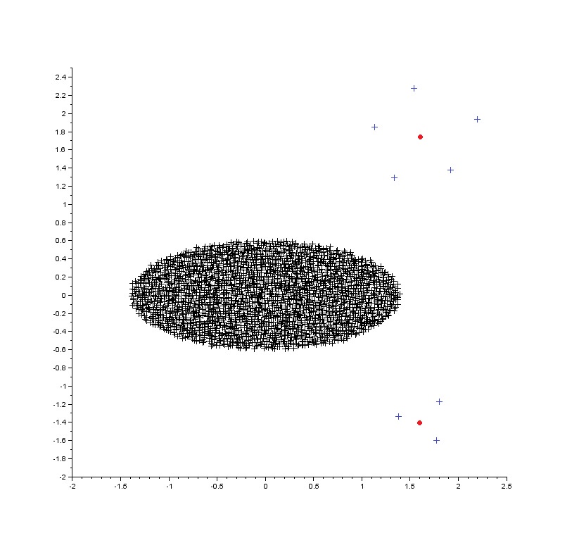
Figure 1. Spectrum of a Gaussian elliptic matrix of size $N=2500$ with perturbation matrix $\mathbf{P}=\operatorname{\text{diag}}\left(\mathbf{R}_{5}(1.5+2.625\operatorname{i}),\mathbf{R}_{3}(1.5-1.5\operatorname{i}),0,\ldots,0\right)$. We see the blue crosses “$+$” (outliers) forming respectively a regular pentagon and an equilateral triangle around the red dots “$\bullet$” (their limit). We also see a significant difference between the two rates of convergence, $N^{-1/10}$ and $N^{-1/6}$.

The general results about asymptotic fluctuations of matrix entries that we prove here are then applied to the fluctuations of the outliers of Gaussian elliptic matrices. One can prove (see e.g. [20]) that the global behavior of the spectrum of a large random matrix is not altered, from the macroscopic point of view, by a low rank additive perturbation. However, some of the eigenvalues, called outliers, can deviate away from the bulk, depending on the strength of the perturbation. Firstly brought to light for empirical covariance matrices by Johnstone in [30], this phenomenon, known as the BBP transition, was proved by Baik, Ben Arous and Péché in [6], and then extended to several Hermitian models in [48, 27, 16, 17, 49, 10, 11, 8, 9, 18, 31, 32]. Non-Hermitian models have been also studied: i.i.d. matrices in [51, 14, 41], real elliptic matrices in [46], matrices from the Single Ring Theorem in [12] and also nearly Hermitian matrices [44, 45]. As an application of our main result, we investigate the fluctuations of the outliers and due to the non-Hermitian structure, we prove, as in [12, 14, 41, 44], that the distribution of the fluctuations highly depends on the shape of the Jordan Canonical Form of the perturbation. In particular, the convergence rates depend on the sizes of the Jordan blocks. Also, the outliers tend to locate around their limits at the vertices of regular polygons (see Figure 1). At last, as in [12], we prove the quite surprising fact that outliers at macroscopic distance from each other can have correlations fluctuations (see Remark 2.20), .

The paper is organized as follows. In Section 2, we state our main results (Theorems 2.1, 2.3, 2.12 and 2.18) and their corollaries. These theorems are then proved in the following sections and an appendix is devoted to a technical result needed here.

Notation: For $u,v$ sequences, $u=o(v)$ means that $u/v\to 0$ and $u=O\left(v\right)$ means that $u/v$ is bounded. Also, the dimension $N$ of the matrices is most times an implicit parameter.

2. Main results

2.1. General results

Let $\mathbf{A}=\big{(}\mathbf{A}_{k}\big{)}_{k\in K}$ be a collection of $N\times N$ random matrices and let $\big{(}\mathbf{M}_{\ell}\big{)}_{\ell\in L}$ be a collection $N\times N$ non random matrices, both implicitly depending on $N$.

Hypothesis 1.

• $\mathbf{A}$ is invariant in distribution under unitary conjugation: for any non random unitary matrix $\mathbf{U}$,

  $$\big{(}\mathbf{A}_{k}\big{)}_{k\in K}\stackrel{{\scriptstyle\text{law}}}{{=}}\big{(}\mathbf{U}\mathbf{A}_{k}\mathbf{U}^{*}\big{)}_{k\in K};$$

• for each $k\in K$, and each $p,q\geq 1$, $\frac{1}{N}\operatorname{Tr}(\mathbf{A}_{k}\mathbf{A}_{k}^{*})^{p}$ is bounded in $L^{q}$ independently of $N$;

• for each $k,k^{\prime}\in K$, we have the following convergences, in $L^{2}$, to deterministic limits:

  $$\lim_{N\to\infty}\frac{1}{N}\operatorname{Tr}\mathbf{A}_{k}\mathbf{A}_{k^{\prime}}-\frac{1}{N}\operatorname{Tr}\mathbf{A}_{k}\cdot\frac{1}{N}\operatorname{Tr}\mathbf{A}_{k^{\prime}}=\tau(k,k^{\prime})$$

  and

  $$\lim_{N\to\infty}\frac{1}{N}\operatorname{Tr}\mathbf{A}_{k}\mathbf{A}_{k^{\prime}}^{*}-\frac{1}{N}\operatorname{Tr}\mathbf{A}_{k}\cdot\frac{1}{N}\operatorname{Tr}\mathbf{A}_{k^{\prime}}^{*}=\tau(k,\overline{k^{\prime}});$$

• for each $\ell,\ell^{\prime}\in L$, we have the following convergences:

  $$\lim_{N\to\infty}\frac{1}{N}\operatorname{Tr}\mathbf{M}_{\ell}\mathbf{M}_{\ell^{\prime}}-\frac{1}{N}\operatorname{Tr}\mathbf{M}_{\ell}\cdot\frac{1}{N}\operatorname{Tr}\mathbf{M}_{\ell^{\prime}}=\eta_{\ell\ell^{\prime}}$$ (3)

  and

  $$\lim_{N\to\infty}\frac{1}{N}\operatorname{Tr}\mathbf{M}_{\ell}\mathbf{M}_{\ell^{\prime}}^{*}-\frac{1}{N}\operatorname{Tr}\mathbf{M}_{\ell}\cdot\frac{1}{N}\operatorname{Tr}\mathbf{M}_{\ell^{\prime}}^{*}=\beta_{\ell\ell^{\prime}}.$$ (4)

Under this sole hypothesis, we first have the following result, focused on the case where the $\mathbf{M}_{\ell}$’s all have null trace, i.e. focused on the projections of the above $\mathbf{A}_{k}$’s onto the space of such matrices.

Theorem 2.1.

Under Hypothesis 1, if, for each $\ell$, $\operatorname{Tr}(\mathbf{M}_{\ell})=0$, then the finite-dimensional marginal distributions of

$$\left(\operatorname{Tr}\big{(}\mathbf{A}_{k}\mathbf{M}_{\ell}\big{)}\right)_{k\in K,\ell\in L}$$ (5)

converge to the ones of a complex centered Gaussian vector $\big{(}\mathcal{G}_{k,\ell}\big{)}_{k\in K,\ell\in L}$ with covariance

$$\operatorname{\mathbb{E}}\left[\mathcal{G}_{k,\ell}{\mathcal{G}_{k^{\prime},\ell^{\prime}}}\right]=\eta_{\ell\ell^{\prime}}\tau(k,k^{\prime}),\qquad\;\text{ and }\qquad\;\operatorname{\mathbb{E}}\left[\mathcal{G}_{k,\ell}\overline{\mathcal{G}_{k^{\prime},\ell^{\prime}}}\right]=\beta_{\ell\ell^{\prime}}\tau(k,\overline{k^{\prime}}).$$

Remark 2.2.

Note that by invariance of the distribution of $\mathbf{A}$ under unitary conjugation, we have

$$\operatorname{\mathbb{E}}\operatorname{Tr}\big{(}\mathbf{A}_{k}\mathbf{M}_{\ell}\big{)}=\operatorname{\mathbb{E}}\big{(}\frac{1}{N}\operatorname{Tr}\mathbf{A}_{k}\big{)}\operatorname{Tr}\mathbf{M}_{\ell},$$

hence the random variables of (5) are centered and the ones of (7) below rewrite

$$\operatorname{Tr}\big{(}\mathbf{A}_{k}\mathbf{M}_{\ell}\big{)}-\operatorname{\mathbb{E}}\big{(}\frac{1}{N}\operatorname{Tr}\mathbf{A}_{k}\big{)}\operatorname{Tr}\mathbf{M}_{\ell}.$$

The following theorem gives the joint fluctuations of the projections of the $\mathbf{A}_{k}$’s on null trace matrices and of their traces.

Hypothesis 2.

The finite-dimensional marginal distributions of the process $\big{(}\operatorname{Tr}\mathbf{A}_{k}-\operatorname{\mathbb{E}}\operatorname{Tr}\mathbf{A}_{k}\big{)}_{k\in K}$ converge to those of a random centered vector $(\mathcal{T}_{k})_{k\in K}$ and for each $\ell\in L$, there is $\alpha_{\ell}\in\operatorname{\mathbb{C}}$ such that

$$\lim_{N\to\infty}\frac{1}{N}\operatorname{Tr}\mathbf{M}_{\ell}=\alpha_{\ell}.$$ (6)

Theorem 2.3.

Under Hypotheses 1 and 2, the finite-dimensional marginal distributions of

$$\left(\operatorname{Tr}\big{(}\mathbf{A}_{k}\mathbf{M}_{\ell}\big{)}-\operatorname{\mathbb{E}}\operatorname{Tr}\big{(}\mathbf{A}_{k}\mathbf{M}_{\ell}\big{)}\right)_{k\in K,\ell\in L}$$ (7)

converge to the ones of $\big{(}\mathcal{G}_{k,\ell}+\alpha_{\ell}\mathcal{T}_{k}\big{)}_{k\in K,\ell\in L}$ where $\big{(}\mathcal{G}_{k,\ell}\big{)}_{k\in K,\ell\in L}$ is a complex centered Gaussian vector independent from $\big{(}\mathcal{T}_{k}\big{)}_{k\in K}$ and with covariance

$$\operatorname{\mathbb{E}}\left[\mathcal{G}_{k,\ell}{\mathcal{G}_{k^{\prime},\ell^{\prime}}}\right]=\eta_{\ell\ell^{\prime}}\tau(k,k^{\prime}),\qquad\;\text{ and }\qquad\;\operatorname{\mathbb{E}}\left[\mathcal{G}_{k,\ell}\overline{\mathcal{G}_{k^{\prime},\ell^{\prime}}}\right]=\beta_{\ell\ell^{\prime}}\tau(k,\overline{k^{\prime}}).$$

A direct consequence of this theorem is the asymptotic independence of the projections of the matrices $\mathbf{A}_{k}$ onto the subspace of null trace matrices from their projections onto the orthogonal of this subspace:

Corollary 2.4.

Under Hypotheses 1 and 2, suppose that for any $\ell\in L$, we have $\operatorname{Tr}(\mathbf{M}_{\ell})=0$. Then the processes

$$\left(\operatorname{Tr}\big{(}\mathbf{A}_{k}\mathbf{M}_{\ell}\big{)}\right)_{k\in K,\ell\in L}\qquad\text{ and }\qquad\big{(}\operatorname{Tr}\mathbf{A}_{k}-\operatorname{\mathbb{E}}\operatorname{Tr}\mathbf{A}_{k}\big{)}_{k\in K}$$

are asymptotically independent.

Remark 2.5.

It has been proved in [36] that unitary invariance implies second order freeness in many cases. However, Theorems 2.1 and 2.3, as well as their corollaries, cannot be deduced from the theory of second order freeness. The reason is that neither the random matrices $\mathbf{A}_{k}$ nor the matrices $\mathbf{M}_{\ell}$ are supposed to have a second order limit. Even in the case where the random matrices $\mathbf{A}_{k}$ have a second order limit (see Section 2.2), the “test matrices” that we consider (i.e. the matrices $\mathbf{M}_{\ell}$) are not supposed to have a second order limit, nor to be well approximated by matrices having a second order limit. For example, if

$$\mathbf{M}_{\ell}=\sqrt{N}\times\text{(an elementary matrix)}$$

(a typical case of application of our results), then for any $p\geq 2$, the sequence

$$\frac{1}{N}\operatorname{Tr}(\mathbf{M}_{\ell}\mathbf{M}_{\ell}^{*})^{p}=N^{p-1}$$

does not have any finite limit as $N\to\infty$, nor is bounded (which would be required to prove our results as application of second order freeness).

2.2. Second-order freeness implies fluctuations of matrix elements

As explained in Remark 2.5, our results do not follow from second order freeness theory. However, we shall see in the following corollary that they extend the consequences of the existence of a second order limit for unitarily invariant matrix ensembles. Let $\operatorname{\mathbb{C}}\langle x_{k},x_{k}^{*},k\in K\rangle$ denote the space of polynomials in the non commutative variables $x_{k},x_{k}^{*}$, indexed by $k\in K$. The following corollary follows directly from Theorem 2.3.

Corollary 2.6.

Let $\big{(}\mathbf{A}_{k}\big{)}_{k\in K}$ be a collection of $N\times N$ random matrices which is invariant by unitary conjugation and which converges in second order $*$-distribution to some family $a=(a_{k})_{k\in K}$ in $(\mathcal{A},\tau_{1},\tau_{2})$ as $N\to\infty$. Let $\big{(}\mathbf{M}_{\ell}\big{)}_{\ell\in L}$ be a collection non random matrices satisfying (3), (4) and (6).

Then the finite-dimensional marginal distributions of

$$\left(\operatorname{Tr}\big{(}P(\mathbf{A})\mathbf{M}_{\ell}\big{)}-\operatorname{\mathbb{E}}\operatorname{Tr}\big{(}P(\mathbf{A})\mathbf{M}_{\ell}\big{)}\right)_{P\in\operatorname{\mathbb{C}}\langle x_{k},x_{k}^{*},k\in K\rangle,\ell\in L}$$ (8)

converge to the ones of a complex centered Gaussian vector

$$\big{(}\mathcal{H}_{P,\ell}\big{)}_{P\in\operatorname{\mathbb{C}}\langle x_{k},x_{k}^{*},k\in K\rangle,\ell\in L}$$

such that, for all $P,Q\in\operatorname{\mathbb{C}}\langle x_{k},x_{k}^{*},k\in K\rangle$ and $\ell,\ell^{\prime}\in L$,

$$\operatorname{\mathbb{E}}{\mathcal{H}_{P,\ell}{\mathcal{H}_{Q,\ell^{\prime}}}} = \alpha_{\ell}\alpha_{\ell^{\prime}}\tau_{2}(P(a),Q(a))+\eta_{\ell\ell^{\prime}}\big{(}\tau_{1}(P(a)Q(a))-\tau_{1}(P(a))\tau_{1}(Q(a))\big{)},$$

$$\operatorname{\mathbb{E}}{\mathcal{H}_{P,\ell}\overline{\mathcal{H}_{Q,\ell^{\prime}}}} = \alpha_{\ell}\overline{\alpha_{\ell^{\prime}}}\tau_{2}(P(a),Q(a)^{*})+\beta_{\ell\ell^{\prime}}\big{(}\tau_{1}(P(a)Q(a)^{*})-\tau_{1}(P(a))\tau_{1}(Q(a)^{*})\big{)}.$$

Remark 2.7.

The following matrices have been shown to converge in second order $*$-distribution:

• Wishart matrices and matrices of the type $\mathbf{U}\mathbf{A}\mathbf{V}$ or $\mathbf{U}\mathbf{A}\mathbf{U}^{*}$, with $\mathbf{U},\mathbf{V}$ independent and Haar distributed on $U(N)$ and $\mathbf{A}$ deterministic with a limit spectral distribution [35, 37, 36, 23]

• GUE matrices or more generally matrix models where the entries interact via a potential [29],

• Ginibre matrices [43],

• random unitary matrices distributed according to the Haar measure on the unitary group $U(N)$ [26],

• matrices arising from the heat kernel measure on $U(N)$ [33] and on $GL_{N}(\mathbb{C})$ [19].

A consequence of Corollary 2.6 is that any non commutative polynomial in independent random matrices taken from the list above has asymptotically Gaussian entries, which are independent modulo a possible symmetry.

2.3. Left and right unitary invariant matrices

Here is another corollary on random matrices invariant by left and right unitary multiplication.

Corollary 2.8.

Let $\mathbf{A}=\big{(}\mathbf{A}_{k}\big{)}_{k\in K}$ be a collection of $N\times N$ random matrices such that:

• $\mathbf{A}$ is invariant, in law, by left and right multiplication by unitary matrices: for any non random unitary matrix $\mathbf{U}$, $\mathbf{A}\stackrel{{\scriptstyle\text{law}}}{{=}}\big{(}\mathbf{U}\mathbf{A}_{k}\big{)}_{k\in K}\stackrel{{\scriptstyle\text{law}}}{{=}}\big{(}\mathbf{A}_{k}\mathbf{U}\big{)}_{k\in K}$;

• for each $k$ and each $p,q$, $\frac{1}{N}\operatorname{Tr}|\mathbf{A}_{k}|^{2p}$ is bounded in $L^{q}$ independently of $N$;

• for each $k,k^{\prime}$, the sequence $\frac{1}{N}\operatorname{Tr}\mathbf{A}_{k}\mathbf{A}_{k^{\prime}}^{*}$ converges in $L^{2}$ to some non random limits denoted $\tau(k,\overline{k^{\prime}})$.

Let $\big{(}\mathbf{M}_{\ell}\big{)}_{\ell\in L}$ be a collection non random matrices satisfying (3), (4) and (6). Then the finite-dimensional marginal distributions of

$$\left(\operatorname{Tr}(\mathbf{A}_{k}\mathbf{M}_{\ell})\right)_{k\in K,\ell\in L}$$

converge to the ones of a complex centered Gaussian vector $\big{(}\mathcal{G}_{k,\ell}\big{)}_{k\in K,\ell\in L}$ with covariance

$$\operatorname{\mathbb{E}}\mathcal{G}_{k,\ell}\mathcal{G}_{k^{\prime},\ell^{\prime}}\ =\ 0, \operatorname{\mathbb{E}}\mathcal{G}_{k,\ell}\overline{\mathcal{G}_{k^{\prime},\ell^{\prime}}}\ =\ \beta_{\ell,\ell^{\prime}}\tau(k,\overline{k^{\prime}}).$$ and

The proof of this corollary is postponed to Section 3.4: we show that the hypotheses of the corollary imply Hypotheses 1 and 2.

2.4. Permutation matrix entries under randomized basis

Let $S$ be a uniform random $N\times N$ permutation matrix. For $T_{d}$ the number of $d$-cycles of the underlying permutation, the distribution of $(T_{d})_{d\geq 1}$ converges as $N\to\infty$ to a Poisson process $(\mathcal{Z}_{d})_{d\geq 1}$ on the set of positive integers with intensity $1/d$ (see [3]). It implies that each trace $\operatorname{Tr}(S^{k})$ ($k\geq 1$) converges in distribution to $\sum_{d|k}d\mathcal{Z}_{d}$. Thanks to Theorem 2.3 and Remark 2.2, we deduce directly the following result about the matrix entries of a uniform permutation matrix $S$ conjugated by a uniform unitary matrix.

Corollary 2.9.

Let $S$ be a $N\times N$ random permutation matrix which is uniformly distributed, $U$ be a $N\times N$ random unitary matrix which is Haar distributed , and $\big{(}\mathbf{M}_{\ell}\big{)}_{\ell\in L}$ a collection of non random matrices satisfying (3), (4) and (6). Then the finite-dimensional marginal distributions of

$$\left(\operatorname{Tr}\big{(}US^{k}U^{*}\mathbf{M}_{\ell}\big{)}\right)_{k\geq 1,\ell\in L}$$

converge to the ones of $\big{(}\mathcal{G}_{k,\ell}+\alpha_{\ell}\sum_{d|k}d\mathcal{Z}_{d}\big{)}_{k\geq 1,\ell\in L}$, where $\big{(}\mathcal{G}_{k,\ell}\big{)}_{k\geq 1,\ell\in L}$ is a complex centered Gaussian vector with covariance

$$\operatorname{\mathbb{E}}\mathcal{G}_{k,\ell}\mathcal{G}_{k^{\prime},\ell^{\prime}}\ =\ 0, \operatorname{\mathbb{E}}\mathcal{G}_{k,\ell}\overline{\mathcal{G}_{k^{\prime},\ell^{\prime}}}\ =\ \mathbbm{1}_{k=k^{\prime}}\beta_{\ell,\ell^{\prime}},$$ and

and $(\mathcal{Z}_{d})_{d\geq 1}$ is a Poisson process on the set of positive integers with intensity $1/d$ which is independent from $\big{(}\mathcal{G}_{k,\ell}\big{)}_{k\in\mathbb{N},\ell\in L}$.

This is to be compared with the results of [52], where the entries of the matrix $S$ conjugated by a uniform random orthogonal matrix are studied.

2.5. Low rank perturbation for Gaussian elliptic matrices

Matrices from the Gaussian elliptic ensemble, first introduced in [50], can be defined as follows.

Definition 2.10.

A Gaussian elliptic matrix of parameter $\rho\in[-1,1]$ is a random matrix $\mathbf{Y}=[y_{ij}]_{i,j=1}^{N}$ such that

• $\{(y_{ij},y_{ji}),1\leq i<j\leq N\}\cup\{y_{ii},1\leq i\leq N\}$ is a family of independent random vectors,

• $\{(y_{ij},y_{ji}),1\leq i<j\leq N\}$ are i.i.d. Gaussian, centered, such that

  $$\operatorname{\mathbb{E}}y_{ij}^{2}=\operatorname{\mathbb{E}}y_{ji}^{2}=\operatorname{\mathbb{E}}y_{ij}\overline{y_{ji}}=0,\quad\operatorname{\mathbb{E}}|y_{ij}|^{2}=\operatorname{\mathbb{E}}|y_{ji}|^{2}=1\ \quad\text{ and }\quad\operatorname{\mathbb{E}}y_{ij}y_{ji}=\rho$$

• $\{y_{ii},1\leq i\leq N\}$ are i.i.d. Gaussian, centered, such that

  $$\operatorname{\mathbb{E}}y_{ii}^{2}=\rho\quad\text{ and }\quad\operatorname{\mathbb{E}}|y_{ii}|^{2}=1.$$

Remark 2.11.

Gaussian elliptic matrices can be seen as an interpolation between GUE matrices and Ginibre matrices. Indeed, a Gaussian elliptic matrix $\mathbf{Y}$ of parameter $\rho$ can be realized as

$$\mathbf{Y}\ =\ \sqrt{\frac{1+\rho}{2}}\mathbf{H}_{1}+\operatorname{i}\sqrt{\frac{1-\rho}{2}}\mathbf{H}_{2},$$

where $\mathbf{H}_{1}$ and $\mathbf{H}_{2}$ are two independent GUE matrices from the GUE. Hence GUE matrices (resp. Ginibre matrices) are Gaussian elliptic matrices of parameter $1$ (resp. $0$).

One can also define more general elliptic random matrices (see [38, 39, 46, 47] for more details). In our case, it is easy to see (using for example Remark 2.11) that the Gaussian elliptic ensemble is invariant in distribution by unitary conjugation, which allows us to use our Theorem 2.3 for this model. In this section, we are interested in the outliers in the spectrum of these matrices. It is known (see [50]) that when you renormalize the matrix $\mathbf{Y}$ by $\sqrt{N}$, its limiting eigenvalue distribution is the uniform measure $\mu_{\rho}$ on the ellipse

$$\mathcal{E}_{\rho}\ :=\ \left\{z\in\operatorname{\mathbb{C}}\ ;\ \frac{(\operatorname{\operatorname{Re}}z)^{2}}{(1+\rho)^{2}}+\frac{(\operatorname{\operatorname{Im}}z)^{2}}{(1-\rho)^{2}}\ \leq\ 1\right\}.$$ (9)

Also, we know that adding a finite rank matrix $\mathbf{P}$ to such a matrix $\mathbf{Y}$ barely alters its spectrum from the global point of view (see [39, Theorem 1.8]), but may give rise to outliers. The generic location of the outliers has already been studied (see [46]), but the authors did not consider the fluctuations.

For all $N\geq 1$, let $\mathbf{X}_{N}:=\frac{1}{\sqrt{N}}\mathbf{Y}_{N}$ where $\mathbf{Y}_{N}$ is an $N\times N$ Gaussian elliptic matrix of parameter $\rho$ and let $\mathbf{P}_{N}$ be a $N\times N$ random matrix independent from $\mathbf{X}_{N}$ whose rank is bounded by an integer $r$ (independent from $N$). We consider the additive pertubation

$$\widetilde{\mathbf{X}}_{N} := \mathbf{X}_{N}+\mathbf{P}_{N}.$$

Since, for any unitary matrix $\mathbf{U}$ which is independent from $\mathbf{X}_{N}$, we have $\mathbf{X}_{N}\overset{(d)}{=}\mathbf{U}\mathbf{X}_{N}\mathbf{U}^{*}$, we can assume that $\mathbf{P}_{N}$ has the following block structure

$$\mathbf{P}_{N} = \begin{pmatrix}\mathbf{P}&0\\ 0&0\end{pmatrix},\ \ \ \ \ \text{ where }\mathbf{P}\text{ is a }2r\times 2r\text{ matrix}$$

(indeed, any complex matrix is unitarily similar to a upper triangular matrix and since the rank of $\mathbf{P}_{N}$ is lower than $r$, we have $\dim(\operatorname{Im}\mathbf{P}_{N}+(\operatorname{Ker}\mathbf{P}_{N})^{\perp})\leq 2r$).

Theorem 2.12 (Outliers for finite rank perturbations of a Gaussian elliptic matrix).

Let $\varepsilon>0$. Suppose that $\mathbf{P}_{N}$ does not have any eigenvalue $\lambda$ such that

$$|\lambda|\ >\ 1\quad\textrm{ and }\quad 1+|\rho|+\varepsilon\ <\ \left|\lambda+\frac{\rho}{\lambda}\right|\ <\ 1+|\rho|+3\varepsilon,$$ (10)

and has exactly $j\leq r$ eigenvalues $\lambda_{1}(\mathbf{P}_{N}),\ldots,\lambda_{j}(\mathbf{P}_{N})$ (counted with multiplicity) such that, for each $i=1,\ldots,j$,

$$|\lambda_{i}(\mathbf{P}_{N})|\ >\ 1\quad\textrm{ and }\quad\left|\lambda_{i}(\mathbf{P}_{N})+\frac{\rho}{\lambda_{i}(\mathbf{P}_{N})}\right|\ >\ 1+|\rho|+3\varepsilon.$$ (11)

Then, with probability tending to one, $\widetilde{\mathbf{X}}_{N}:=\mathbf{X}_{N}+\mathbf{P}_{N}$ possesses exactly $j$ eigenvalues $\widetilde{\lambda}_{1},\ldots,\widetilde{\lambda}_{j}$ in $\{z\in\operatorname{\mathbb{C}}\,;\,|z|>1+|\rho|+2\varepsilon\}$ and after a proper labeling

$$\widetilde{\lambda}_{i}\ =\ \lambda_{i}(\mathbf{P}_{N})+\frac{\rho}{\lambda_{i}(\mathbf{P}_{N})}+o\left(1\right),$$ (12)

for each $1\leq i\leq j$.

Remark 2.13.

In [46], the authors prove this result for real elliptic random matrices and have a more precise statement. Indeed, they replace in our conditions (10) and (11) the annulus $\{z\in\operatorname{\mathbb{C}}\,;\,1+|\rho|+\varepsilon<|z|<1+|\rho|+3\varepsilon\}$ (resp. $\{z\in\operatorname{\mathbb{C}},\ |z|>1+|\rho|+3\varepsilon\}$) by $\mathcal{E}_{\rho,3\varepsilon}\backslash\mathcal{E}_{\rho,\varepsilon}$ (resp. by $\mathcal{E}_{\rho,3\varepsilon}^{c}$) where $\mathcal{E}_{\rho,\varepsilon}$ is a $\varepsilon$-neighborhood of the ellipse $\mathcal{E}_{\rho}$ (see (9)). Our proof relies on the identity

$$\operatorname{Tr}\left(z-\mathbf{X}\right)^{-1}\ =\ \sum_{k\geq 0}z^{-k-1}\operatorname{Tr}\mathbf{X}^{k},$$

which is true only when $|z|$ is larger than the spectral radius of $X$, this is why (10) and (11) are circular conditions, instead of elliptic ones.

To study the fluctuations of the outliers $\widetilde{\lambda}_{i}$ around their generic locations as given by (12), we need to specify the shape of the matrix $\mathbf{P}$ as it is done in [12]. Indeed, since $\mathbf{P}$ is not Hermitian, we need to introduce its Jordan Canonical Form (JCF) which is supposed to be independent of $N$, but for its kernel part. We know that, in a proper basis, $\mathbf{P}$ is a direct sum of Jordan blocks, i.e. blocks of the form

$$\mathbf{R}_{p}(\theta) = \begin{pmatrix}\theta&1&&(0)\\ &\ddots&\ddots&\\ \lx@intercol\hfil\hbox{\multirowsetup(0)}\hfil\lx@intercol&\ddots&1\\ \lx@intercol\hfil\hfil\lx@intercol&&\theta\end{pmatrix}\ \in\ \operatorname{\mathbb{C}}^{p\times p},\qquad\theta\in\operatorname{\mathbb{C}},\,p\geq 1$$ (13)

Let us denote by $\theta_{1},\ldots,\theta_{q}$ the distinct eigenvalues of $\mathbf{P}$ satisfying condition (11). For convenience, we shall write from now on

$$\hat{\theta}_{i} := \theta_{i}+\frac{\rho}{\theta_{i}}.$$ (14)

We introduce a positive integer $\alpha_{i}$, some positive integers $p_{i,1}>\cdots>p_{i,\alpha_{i}}$ corresponding to the distinct sizes of the blocks relative to the eigenvalue $\theta_{i}$ and $\beta_{i,1},\ldots,\beta_{i,\alpha_{i}}$ such that for all $j$, $\mathbf{R}_{p_{i,j}}(\theta_{i})$ appears $\beta_{i,j}$ times, so that, for a certain $2r\times 2r$ invertible matrix $\mathbf{Q}$, we have:

$$\mathbf{J} = \mathbf{Q}^{-1}\mathbf{P}\mathbf{Q}\ =\ \Bigg{(}\bigoplus_{i=1}^{q}\ \bigoplus_{j=1}^{\alpha_{i}}\!\underbrace{\begin{pmatrix}\mathbf{R}_{p_{i,j}}(\theta_{i})&&\\ &\ddots&\\ &&\mathbf{R}_{p_{i,j}}(\theta_{i})\end{pmatrix}}_{\beta_{{i,j}}\textrm{ blocks}}\Bigg{)}\ \bigoplus\ \hat{\mathbf{P}}$$ (15)

where $\oplus$ is defined, for square block matrices, by $\mathbf{M}\oplus\mathbf{N}:=\begin{pmatrix}\mathbf{M}&0\\ 0&\mathbf{N}\end{pmatrix}$ and $\hat{\mathbf{P}}$ is a matrix whose eigenvalues $\theta$ are such that $|\theta|<1$ or $|\theta+\rho\theta^{-1}|<1+\rho+\varepsilon$.
The asymptotic orders of the fluctuations of the eigenvalues of $\mathbf{X}_{N}+\mathbf{P}_{N}$ depend on the sizes $p_{i,j}$ of the blocks. We know, by Theorem 2.12, that there are $\sum_{j=1}^{\alpha_{i}}p_{ij}\times\beta_{i,j}$ eigenvalues ${\widetilde{\lambda}}$ of $\mathbf{X}_{N}+\mathbf{P}_{N}$ which tend to $\hat{\theta_{i}}=\theta_{i}+\rho\theta_{i}^{-1}$: we shall write them with a $\hat{\theta_{i}}$ on the top left corner, as follows

$${\vphantom{{\widetilde{\lambda}}}}^{\hat{\theta}_{i}}{\widetilde{\lambda}}.$$

Theorem 2.18 below will state that, for each block with size $p_{i,j}$ corresponding to $\theta_{i}$ in the JCF of $\mathbf{P}$, there are $p_{i,j}$ eigenvalues (we shall write them with $p_{i,j}$ on the bottom left corner: ${\vphantom{{\widetilde{\lambda}}}}^{\;\;\hat{\theta}_{i}}_{p_{i,j}}{\widetilde{\lambda}}$) whose convergence rate will be $N^{-1/(2p_{i,j})}$. As there are $\beta_{{i,j}}$ blocks of size $p_{i,j}$, there are actually $p_{i,j}\times\beta_{{i,j}}$ eigenvalues tending to $\hat{\theta}_{i}$ with convergence rate $N^{-1/(2p_{i,j})}$ (we shall write them ${\vphantom{{\widetilde{\lambda}}_{s,t}}}^{\;\;\hat{\theta}_{i}}_{p_{i,j}}{\widetilde{\lambda}}_{s,t}$ with $s\in\{1,\ldots,p_{i,j}\}$ and $t\in\{1,\ldots,\beta_{{i,j}}\}$). It would be convenient to denote by $\Lambda_{i,j}$ the vector with size $p_{i,j}\times\beta_{{i,j}}$ defined by

$$\Lambda_{i,j}\ :=\ \displaystyle\left(N^{1/(2p_{i,j})}\cdot\Big{(}{\vphantom{{\widetilde{\lambda}}_{s,t}}}^{\;\;\hat{\theta}_{i}}_{p_{i,j}}{\widetilde{\lambda}}_{s,t}-\hat{\theta}_{i}\Big{)}\right)_{\begin{subarray}{c}1\leq s\leq p_{i,j}\\ 1\leq t\leq\beta_{i,j}\end{subarray}}.$$ (16)

As in [12], we define now the family of random matrices that we shall use to characterize the limit distribution of the $\Lambda_{i,j}$’s. For each $i=1,\ldots,q$, let $I(\theta_{i})$ (resp. $J(\theta_{i})$) denote the set, with cardinality $\sum_{j=1}^{\alpha_{i}}\beta_{i,j}$, of indices in $\{1,\ldots,2r\}$ corresponding to the first (resp. last) columns of the blocks $\mathbf{R}_{p_{i,j}}(\theta_{i})$ ($1\leq j\leq\alpha_{i}$) in (15).

Remark 2.14.

Note that the columns of $\mathbf{Q}$ (resp. of $(\mathbf{Q}^{-1})^{*}$) whose index belongs to $I(\theta_{i})$ (resp. $J(\theta_{i})$) are eigenvectors of $\mathbf{P}$ (resp. of $\mathbf{P}^{*}$) associated to $\theta_{i}$ (resp. $\overline{\theta_{i}}$). See [12, Remark 2.8].

Now, let

$$\left({m}^{\theta_{i}}_{k,\ell}\right)_{\begin{subarray}{c}1\leq i\leq q_{\hphantom{1.}}\quad\quad\ \ \\ (k,\ell)\in J(\theta_{i})\times I(\theta_{i})\end{subarray}}$$ (17)

be the random centered complex Gaussian vector with covariance

$$\begin{array}[]{rcl}\operatorname{\mathbb{E}}\left[m_{k,\ell}^{\theta_{i}}m_{k^{\prime},\ell^{\prime}}^{\theta_{i^{\prime}}}\right]&=&\displaystyle\Big{(}\frac{1}{\theta_{i}\theta_{i^{\prime}}-\rho}-\frac{1}{\theta_{i}\theta_{i^{\prime}}}\Big{)}\delta_{k,\ell^{\prime}}\delta_{k^{\prime},\ell}\\ \operatorname{\mathbb{E}}\left[m_{k,\ell}^{\theta_{i}}\overline{m_{k^{\prime},\ell^{\prime}}^{\theta_{i^{\prime}}}}\right]&=&\displaystyle\Phi_{\rho}(\hat{\theta_{i}},\hat{\theta}_{{i^{\prime}}})\mathbf{e}_{k}\mathbf{Q}^{-1}(\mathbf{Q}^{-1})^{*}\mathbf{e}_{k^{\prime}}\cdot\mathbf{e}_{\ell^{\prime}}\mathbf{Q}^{*}\mathbf{Q}\mathbf{e}_{\ell},\end{array}$$ (20)

where $\mathbf{e}_{1},\ldots,\mathbf{e}_{2r}$ are the column vectors of the canonical basis of $\operatorname{\mathbb{C}}^{2r}$ and

$$\Phi_{\rho}(z,z^{\prime}) = \int\frac{1}{z-w}\frac{1}{\overline{z^{\prime}}-\overline{w}}\mu_{\rho}(\mathrm{d}w)-\int\frac{1}{z-w}\mu_{\rho}(\mathrm{d}w)\int\frac{1}{\overline{z^{\prime}}-\overline{w}}\mu_{\rho}(\mathrm{d}w).$$

Remark 2.15.

In Section 3.5, the random vector of (17) will appear as limit in the convergence:

$$\left(\sqrt{N}\mathbf{e}_{k}^{*}\mathbf{Q}^{-1}\left(\left(\hat{\theta}_{i}-\mathbf{X}_{N}\right)^{-1}-\frac{1}{\theta_{i}}\right)\mathbf{Q}\mathbf{e}_{\ell}\right)_{\begin{subarray}{c}1\leq i\leq q_{\hphantom{1.}}\quad\quad\ \ \\ (k,\ell)\in J(\theta_{i})\times I(\theta_{i})\end{subarray}}\ {\operatorname{\overset{(d)}{\longrightarrow}}}\ \left({m}^{\theta_{i}}_{k,\ell}\right)_{\begin{subarray}{c}1\leq i\leq q_{\hphantom{1.}}\quad\quad\ \ \\ (k,\ell)\in J(\theta_{i})\times I(\theta_{i})\end{subarray}}\,.$$

This convergence is a consequence of Theorem 2.3.

Remark 2.16.

When $\rho=0$, one has

$$\Phi_{0}(z,z^{\prime}) = \frac{1}{\pi}\int_{|w|\leq 1}\frac{1}{z-w}\frac{1}{\overline{z^{\prime}}-\overline{w}}\mathrm{d}w-\frac{1}{\pi}\int_{|w|\leq 1}\frac{1}{z-w}\mathrm{d}w\frac{1}{\pi}\int_{|w|\leq 1}\frac{1}{\overline{z^{\prime}}-\overline{w}}\mathrm{d}w$$

$$= \frac{1}{z\overline{z^{\prime}}-1}-\frac{1}{z\overline{z^{\prime}}}\ =\ \frac{1}{z\overline{z^{\prime}}(z\overline{z^{\prime}}-1)}.$$

We recover the expression of the covariance in the Ginibre case (see [12]). Also, the expression of $\Phi_{1}$ corresponds to the covariance in the GUE case (see [44]).

For each $i,j$, let $K(i,j)$ (resp. $K(i,j)^{-}$) be the set, with cardinality $\beta_{i,j}$ (resp. $\sum_{j^{\prime}=1}^{j-1}\beta_{i,j^{\prime}}$), of indices in $J(\theta_{i})$ corresponding to a block of the type $\mathbf{R}_{p_{i,j}}(\theta_{i})$ (resp. to a block of the type $\mathbf{R}_{p_{i,j^{\prime}}}(\theta_{i})$ for $j^{\prime}<j$). In the same way, let $L(i,j)$ (resp. $L(i,j)^{-}$) be the set, with the same cardinality as $K(i,j)$ (resp. as $K(i,j)^{-}$), of indices in $I(\theta_{i})$ corresponding to a block of the type $\mathbf{R}_{p_{i,j}}(\theta_{i})$ (resp. to a block of the type $\mathbf{R}_{p_{i,j^{\prime}}}(\theta_{i})$ for $j^{\prime}<j$). Note that $K(i,j)^{-}$ and $L(i,j)^{-}$ are empty if $j=1$. Let us define the random matrices

$$\operatorname{M}^{\theta_{i},\mathrm{I}}_{j}\ :=\ [m^{\theta_{i},n}_{k,\ell}]_{{}^{k\in K(i,j)^{-}}_{\ell\in L(i,j)^{-}}} \operatorname{M}^{\theta_{i},\mathrm{I}\mathrm{I}}_{j}\ :=\ [m^{\theta_{i}}_{k,\ell}]_{{}^{k\in K(i,j)^{-}}_{\ell\in L(i,j)}}$$

$$\operatorname{M}^{\theta_{i},\mathrm{I}\mathrm{I}\mathrm{I}}_{j,n}\ :=\ [m^{\theta_{i}}_{k,\ell}]_{{}^{k\in K(i,j)}_{\ell\in L(i,j)^{-}}} \operatorname{M}^{\theta_{i},\mathrm{I}\mathrm{V}}_{j}\ :=\ [m^{\theta_{i},n}_{k,\ell}]_{{}^{k\in K(i,j)}_{\ell\in L(i,j)}}$$

and then let us define the matrix ${\mathbf{M}}^{\theta_{i}}_{j}$ as

$$\mathbf{M}^{\theta_{i}}_{j}\ :=\ \theta_{i}\left(\operatorname{M}^{\theta_{i},\mathrm{I}\mathrm{V}}_{j}-\operatorname{M}^{\theta_{i},\mathrm{I}\mathrm{I}\mathrm{I}}_{j}\left(\operatorname{M}^{\theta_{i},\mathrm{I}}_{j}\right)^{-1}\operatorname{M}^{\theta_{i},\mathrm{I}\mathrm{I}}_{j}\right)$$ (22)

Remark 2.17.

It follows from the fact that the matrix $\mathbf{Q}$ is invertible that $\operatorname{M}^{\theta_{i},\mathrm{I}}_{j}$ is a.s. invertible and that so is $\mathbf{M}^{\theta_{i}}_{j}$.

Now, we can state the result about the fluctuations of the outliers.

Theorem 2.18.

1. As $N$ goes to infinity, the random vector

   $$\left(\Lambda_{i,j}\right)_{\begin{subarray}{c}1\leq i\leq q_{\hphantom{1}}\\ 1\leq j\leq\alpha_{i}\end{subarray}}$$

   defined at (16) converges in distribution to a random vector

   $$\left(\Lambda^{\infty}_{i,j}\right)_{\begin{subarray}{c}1\leq i\leq q_{\hphantom{1}}\\ 1\leq j\leq\alpha_{i}\end{subarray}}$$

   with joint distribution defined by the fact that, for each $1\leq i\leq q$ and $1\leq j\leq\alpha_{i}$, $\Lambda_{i,j}^{\infty}$ is the collection of the ${p_{i,j}}^{\textrm{th}}$ roots of the eigenvalues of the random matrix $\mathbf{M}^{\theta_{i}}_{j}$.

2. The distributions of the random matrices $\mathbf{M}^{\theta_{i}}_{j}$ are absolutely continuous with respect to the Lebesgue measure and the random vector $\displaystyle\left(\Lambda^{\infty}_{i,j}\right)_{{}^{1\leq i\leq q}_{1\leq j\leq\alpha_{i}}}$ has no deterministic coordinate.

Remark 2.19.

Each non zero complex number has exactly $p_{i,j}$ ${p_{i,j}}^{\textrm{th}}$ roots, drawing a regular $p_{i,j}$-sided polygon. Moreover, by the second part of the theorem, the spectrums of the $\mathbf{M}^{\theta_{i}}_{j}$’s almost surely do not contain $0$, so each $\Lambda_{i,j}^{\infty}$ is actually a complex random vector with $p_{i,j}\times\beta_{i,j}$ coordinates, which draw $\beta_{i,j}$ regular $p_{i,j}$-sided polygons.

Remark 2.20.

We notice that in the particular case where the matrix $\mathbf{Q}$ is unitary, the covariance of the Gaussian variables $\left({m}^{\theta_{i}}_{k,\ell}\right)_{\begin{subarray}{c}1\leq i\leq q_{\hphantom{1.}}\quad\quad\ \ \\ (k,\ell)\in J(\theta_{i})\times I(\theta_{i})\end{subarray}}$ can be rewritten

$$\operatorname{\mathbb{E}}\left[m_{k,\ell}^{\theta_{i}}m_{k^{\prime},\ell^{\prime}}^{\theta_{i^{\prime}}}\right] = \displaystyle\Big{(}\frac{1}{\theta_{i}\theta_{i^{\prime}}-\rho}-\frac{1}{\theta_{i}\theta_{i^{\prime}}}\Big{)}\delta_{k,\ell^{\prime}}\delta_{k^{\prime},\ell},$$

$$\operatorname{\mathbb{E}}\left[m_{k,\ell}^{\theta_{i}}\overline{m_{k^{\prime},\ell^{\prime}}^{\theta_{i^{\prime}}}}\right] = \displaystyle\Phi(\hat{\theta}_{i},\hat{\theta}_{i^{\prime}})\delta_{k,k^{\prime}}\delta_{\ell,\ell^{\prime}}.$$

Which means that for any $i,i^{\prime}$ such that $i\neq i^{\prime}$, the familly $\left({m}^{\theta_{i}}_{k,\ell}\right)_{(k,\ell)\in J(\theta_{i})\times I(\theta_{i})}$ is independent from $\left({m}^{\theta_{i^{\prime}}}_{k,\ell}\right)_{(k,\ell)\in J(\theta_{i^{\prime}})\times I(\theta_{i^{\prime}})}$. Indeed, since the Jordan blocks associated to $\theta_{i}$ are distinct from those associated to $\theta_{i^{\prime}}$, the sets $I(\theta_{i})$ and $J(\theta_{i})$ don’t share any common index with $I(\theta_{i^{\prime}})$ and $J(\theta_{i^{\prime}})$. We can deduce that in this particular case, all the fluctuations around $\theta_{i}$ are independent from those around $\theta_{i^{\prime}}$ (see [12, section 2.3.1.] for more details).
However, in the general case, there is no particular reason to have independance between the fluctuations around two spikes at macroscopique distance. To illustrate this phenomenon, we can take the same particular example than [12, Example 2.17] since a Ginibre matrix is also a Gaussian elliptic matrix. In this example, the authors of [12] took a matrix $\mathbf{P}$ of the form

$$\mathbf{P}\ =\ \mathbf{Q}\begin{pmatrix}\theta&0\\ 0&\theta^{\prime}\end{pmatrix}\mathbf{Q}^{-1},\ \quad\quad\ \mathbf{Q}\ =\ \begin{pmatrix}1&\kappa\\ \kappa&1\end{pmatrix},\ \ \ \kappa\neq\pm 1,$$

and they empirically confirmed that, in the case $\kappa\neq 0$, the fluctuations of the outliers around $\theta$ are correlated with these around $\theta^{\prime}$.

3. Proofs of Theorem 2.1 and Theorem 2.3

3.1. Preliminary result

Let $\big{(}\mathbf{B}_{k}\big{)}_{k\in K}$ be a collection of (implicitly depending on $N$) $N\times N$ random matrices such that

• for each $k\in K$, almost surely, $\operatorname{Tr}\mathbf{B}_{k}=0$;

• for each $k\in K$, and each $p,q\geq 1$, $\frac{1}{N}\operatorname{Tr}|\mathbf{B}_{k}|^{2p}$ is bounded in $L^{q}$ independently of $N$;

• for each $k,k^{\prime}\in K$, we have the following convergences to nonrandom variables in $L^{2}$

  $$\lim_{N\to\infty}\frac{1}{N}\operatorname{Tr}\mathbf{B}_{k}\mathbf{B}_{k^{\prime}}=\tau(k,k^{\prime})\ \text{ and }\lim_{N\to\infty}\frac{1}{N}\operatorname{Tr}\mathbf{B}_{k}\mathbf{B}_{k^{\prime}}^{*}=\tau(k,\overline{k^{\prime}}).$$

Let also $\big{(}\mathbf{M}_{\ell}\big{)}_{\ell\in L}$ be a collection non random matrices such that

• for each $\ell,\ell^{\prime}\in L$, we have the following convergences

  $$\lim_{N\to\infty}\frac{1}{N}\operatorname{Tr}\mathbf{M}_{\ell}\mathbf{M}_{\ell^{\prime}}-\frac{1}{N}\operatorname{Tr}\mathbf{M}_{\ell}\cdot\frac{1}{N}\operatorname{Tr}\mathbf{M}_{\ell^{\prime}}=\eta_{\ell\ell^{\prime}}$$

  and

  $$\lim_{N\to\infty}\frac{1}{N}\operatorname{Tr}\mathbf{M}_{\ell}\mathbf{M}_{\ell^{\prime}}^{*}-\frac{1}{N}\operatorname{Tr}\mathbf{M}_{\ell}\cdot\frac{1}{N}\operatorname{Tr}\mathbf{M}_{\ell^{\prime}}^{*}=\beta_{\ell\ell^{\prime}}.$$

At last, let $\mathbf{U}=\mathbf{U}^{(N)}$ be an $N\times N$ Haar-distributed unitary random matrix independent of $\big{(}\mathbf{B}_{k}\big{)}_{k\in K}$.

Proposition 3.1.

Let us fix $p\geq 1$, $(k_{1},\ldots,k_{p})\in K^{p}$ and $(\ell_{1},\ldots,\ell_{p})\in L^{p}$. If $(i)$, $(ii)$, $(iii)$ and $(iv)$ hold, then the centered vector

$$\left(\operatorname{Tr}\big{(}\mathbf{U}\mathbf{B}_{k_{i}}\mathbf{U}^{*}\mathbf{M}_{\ell_{i}}\big{)}\right)_{1\leq i\leq p}$$ (23)

converges in distribution, as $N\to\infty$, to a complex centered Gaussian vector $\big{(}\mathcal{G}_{i}\big{)}_{1\leq i\leq p}$ such that, for all $i,i^{\prime}$,

$$\operatorname{\mathbb{E}}{\mathcal{G}_{i}{\mathcal{G}_{i^{\prime}}}}=\eta_{\ell_{i}\ell_{i^{\prime}}}\tau({k_{i}},{k_{i^{\prime}}}),\ \text{ and }\ \operatorname{\mathbb{E}}{\mathcal{G}_{i}\overline{\mathcal{G}_{i^{\prime}}}}=\beta_{\ell_{i}\ell_{i^{\prime}}}\tau({k_{i}},\overline{k_{i^{\prime}}}).$$

Besides, for any sequence $(Y_{N})$ of bounded random variables such that

• $Y_{N}$ is independent of $\mathbf{U}^{(N)}$,

• $\operatorname{\mathbb{E}}Y_{N}$ has a limit $L_{Y}$

and any polynomial $f$ in $p$ complex variables and their conjugates, we have

$$\lim_{N\to\infty}\operatorname{\mathbb{E}}\left[Y_{N}f\left(\operatorname{Tr}\big{(}\mathbf{U}\mathbf{B}_{k_{i}}\mathbf{U}^{*}\mathbf{M}_{\ell_{i}}\big{)},1\leq i\leq p\right)\right]\;=\;L_{Y}\operatorname{\mathbb{E}}\left[f\left(\mathcal{G}_{i},1\leq i\leq p\right)\right].$$

Proof. First, we can suppose the $\mathbf{B}_{k}$’s and the $\mathbf{M}_{\ell}$’s are all Hermitian (which makes the entries of the vector of (23) real), up to changing

$$\left(\mathbf{B}_{k}\right)_{k\in K} \longrightarrow \left(\mathbf{B}_{(k,1)}:=\frac{1}{2}\big{(}\mathbf{B}_{k}+\mathbf{B}_{k}^{*}\big{)},\;\;\mathbf{B}_{(k,2)}:=\frac{1}{2\mathrm{i}}\big{(}\mathbf{B}_{k}-\mathbf{B}^{*}_{k}\big{)}\right)_{(k,\varepsilon)\in K\times\{1,2\}},$$

$$\left(\mathbf{M}_{\ell}\right)_{\ell\in L} \longrightarrow \left(\mathbf{M}_{(\ell,1)}:=\frac{1}{2}\big{(}\mathbf{M}_{\ell}+\mathbf{M}_{\ell}^{*}\big{)},\;\;\mathbf{M}_{(\ell,2)}:=\frac{1}{2\mathrm{i}}\big{(}\mathbf{M}_{\ell}-\mathbf{M}^{*}_{\ell}\big{)}\right)_{(\ell,\varepsilon)\in L\times\{1,2\}}.$$

Second, as all $\mathbf{B}_{k}$’s have null trace, up to changing $\mathbf{M}_{\ell}\to\mathbf{M}_{\ell}-\frac{1}{N}\operatorname{Tr}\mathbf{M}_{\ell}$, one can suppose that all $\mathbf{M}_{\ell}$’s have null trace.

To prove the full proposition, it suffices to prove the convergence

$$\lim_{N\to\infty}\operatorname{\mathbb{E}}\left[Y_{N}\prod_{i=1}^{n}\operatorname{Tr}\big{(}\mathbf{U}\mathbf{B}_{k_{i}}\mathbf{U}^{*}\mathbf{M}_{\ell_{i}}\big{)}\right]\;=\;L_{Y}\operatorname{\mathbb{E}}\left[\prod_{i=1}^{n}\mathcal{H}_{i}\right].$$

for any $n\geq 1$, $(k_{1},\ldots,k_{n})\in K^{n}$, $(\ell_{1},\ldots,\ell_{n})\in L^{n}$ and any sequence $(Y_{N})$ of bounded random variables independent from $\mathbf{U}^{(N)}$ such that $\lim_{N\to\infty}\operatorname{\mathbb{E}}Y_{N}=L_{Y}$. Indeed, we can take each $k$ as many times as we want in $(k_{1},\ldots,k_{n})$ (and the same for $\ell$), which implies the convergence of the expectation of any polynomials as wanted and consequently the convergence in distribution of finite dimensional marginals.

Let $n\geq 1$, and $\mathfrak{S}_{n}$ be the $n$-th symmetric group, and $\mathfrak{S}_{n,2}$ be the subset of permutations in $\mathfrak{S}_{n}$ with only cycles of length $2$. We denote be $\#\sigma$ the number of cycles of $\sigma\in\mathfrak{S}_{n}$ and by $\operatorname{Fix}(\sigma)$ the number of fixed points of $\sigma$. The neutral element of $\mathfrak{S}_{n}$ is denoted by $\operatorname{id}_{n}$. For any $\sigma\in\mathfrak{S}_{n}$, we set

$$\operatorname{Tr}_{\sigma}\big{(}\mathbf{N}_{i}\big{)}_{i=1}^{n}\ =\ \prod_{\begin{subarray}{c}(t_{1}t_{2}\cdots t_{m})\\ \text{cycle of }\sigma\end{subarray}}\operatorname{Tr}\big{(}\mathbf{N}_{t_{1}}\mathbf{N}_{t_{2}}\cdots\mathbf{N}_{t_{m}}\big{)}$$

For example, for $\sigma\in\mathfrak{S}_{6}$, $\sigma:=(1,2,3,4,5,6)\ \mapsto\ (3,2,4,1,6,5)$

$$\operatorname{Tr}_{\sigma}\big{(}\mathbf{N}_{i}\big{)}_{i=1}^{6}\ =\ \operatorname{Tr}\big{(}\mathbf{N}_{1}\mathbf{N}_{3}\mathbf{N}_{4}\big{)}\operatorname{Tr}\big{(}\mathbf{N}_{2}\big{)}\operatorname{Tr}\big{(}\mathbf{N}_{5}\mathbf{N}_{6}\big{)}.$$

Lemma 3.2.

Let $n\geq 1$, $(k_{1},\ldots,k_{n})\in K^{n}$, $(\ell_{1},\ldots,\ell_{n})\in L^{n}$, and $(Y_{N})$ be any sequence of bounded random variables such that $\lim_{N\to\infty}\operatorname{\mathbb{E}}Y_{N}=L_{Y}$. With the above assumptions on $(\mathbf{M}_{\ell})_{\ell\in L}$ and $(\mathbf{B}_{k})_{k\in K}$, we have, for all $\gamma$ and $\sigma$ in $\mathfrak{S}_{n}$,

$$\operatorname{Tr}_{\gamma}\big{(}\mathbf{M}_{\ell_{i}}\big{)}_{i=1}^{n}\ =\ \mathbbm{1}_{\operatorname{Fix}(\gamma)=0}\,\times\,O\left(N^{n/2}\right)$$

and

$$\operatorname{\mathbb{E}}\left[Y_{N}{\operatorname{Tr}_{\sigma}\big{(}\mathbf{B}_{k_{i}}\big{)}_{i=1}^{n}}\right]\ =\ \mathbbm{1}_{\sigma\in\mathfrak{S}_{n,2}}N^{n/2}L_{Y}\prod_{\begin{subarray}{c}(i,j)\\ \text{cycle of }\sigma\end{subarray}}\tau(k_{i},k_{j})+o(N^{n/2}).$$

Proof. Because $\mathbf{B}_{k}$’s and $\mathbf{M}_{\ell}$’s have null traces, the formulas are true in presence of fixed points. Thus, we can assume that $\sigma$ and $\gamma$ have no fixed point.

The first result comes from Lemma 3.5 and from the fact that, for each $\ell$, $\operatorname{Tr}\mathbf{M}_{\ell}^{2}\ =\ O\left(N\right).$

The second result can be proved in two steps. First, if $\sigma\notin\mathfrak{S}_{n,2}$, the non-commutative Hölder’s inequality (see [1, Appendix A.3]) and Hypothesis (ii) say us that

$$\left|\operatorname{\mathbb{E}}\left[Y_{N}{\operatorname{Tr}_{\sigma}\big{(}\mathbf{B}_{k_{i_{j}}}\big{)}_{j=1}^{n}}\right]\right|=O(N^{\#\sigma})=o(N^{n/2}).$$

If $\sigma\in\mathfrak{S}_{n,2}$ (and $n>0$ is even), we decompose $\sigma$ in $2$-cycles $\sigma\ =\ (i_{1}\ j_{1})\cdots(i_{n/2}\ j_{n/2})$. By classical Hölder’s inequality, the absolute difference between

$$N^{-n/2}\operatorname{\mathbb{E}}\left[Y_{N}{\operatorname{Tr}_{\sigma}\big{(}\mathbf{B}_{k_{j}}\big{)}_{j=1}^{n}}\right]=\operatorname{\mathbb{E}}\left[Y_{N}\prod_{t=1}^{n/2}\frac{1}{N}\operatorname{Tr}\mathbf{B}_{k_{i_{t}}}\mathbf{B}_{k_{j_{t}}}\right]\text{and }\operatorname{\mathbb{E}}\left[Y_{N}\prod_{t=1}^{n/2-1}\frac{1}{N}\operatorname{Tr}\mathbf{B}_{k_{i_{t}}}\mathbf{B}_{k_{j_{t}}}\right]\operatorname{\mathbb{E}}\left[\frac{1}{N}\operatorname{Tr}\mathbf{B}_{k_{i_{1}}}\mathbf{B}_{k_{j_{1}}}\right]$$

is less than

$$\operatorname{\mathbb{E}}[Y_{N}^{2n}]^{1/2n}\prod_{t=1}^{n/2-1}\operatorname{\mathbb{E}}\left[\left(\frac{1}{N}\operatorname{Tr}\mathbf{B}_{k_{i_{t}}}\mathbf{B}_{k_{j_{t}}}\right)^{2n}\right]^{1/2n}\operatorname{\mathbb{V}ar}\left(\frac{1}{N}\operatorname{Tr}\mathbf{B}_{k_{i_{1}}}\mathbf{B}_{k_{j_{1}}}\right)$$

and consequently converges to $0$ - using again the non-commutative Hölder’s inequality (see [1, Appendix A.3]) and Hypothesis (ii) to control $\operatorname{\mathbb{E}}(\frac{1}{N}\operatorname{Tr}\mathbf{B}_{k_{i_{t}}}\mathbf{B}_{k_{j_{t}}})^{2n}$. By a direct induction on $n/2$, it means that the expectation of product

$$N^{-n/2}\operatorname{\mathbb{E}}\left[Y_{N}{\operatorname{Tr}_{\sigma}\big{(}\mathbf{B}_{k_{j}}\big{)}_{j=1}^{n}}\right]=\operatorname{\mathbb{E}}\left[Y_{N}\prod_{t=1}^{n/2}\frac{1}{N}\operatorname{Tr}\mathbf{B}_{k_{i_{t}}}\mathbf{B}_{k_{j_{t}}}\right]$$

has the same limit as the product of expectation

$$\operatorname{\mathbb{E}}\left[Y_{N}\right]\prod_{t=1}^{n/2}\operatorname{\mathbb{E}}\left[\frac{1}{N}\operatorname{Tr}\mathbf{B}_{k_{i_{t}}}\mathbf{B}_{k_{j_{t}}}\right],$$

and the result follows. $\square$
Let $n\geq 1$, $(k_{1},\ldots,k_{n})\in K^{n}$, $(\ell_{1},\ldots,\ell_{n})\in L^{n}$, and $(Y_{N})$ be any sequence of bounded random variables such that $\lim_{N\to\infty}\operatorname{\mathbb{E}}Y_{N}=L$. Using [36, Proposition 3.4] (and, first, an integration with respect to the randomness of $\mathbf{U}$, and then a “full expectation”), we have

$$\operatorname{\mathbb{E}}\left[Y_{N}\prod_{i=1}^{n}\operatorname{Tr}\big{(}\mathbf{U}\mathbf{B}_{k_{i}}\mathbf{U}^{*}\mathbf{M}_{\ell_{i}}\big{)}\right] = \sum_{\sigma,\gamma\in\mathfrak{S}_{n}}\operatorname{Wg}(\sigma\gamma^{-1})\operatorname{\mathbb{E}}[Y_{N}\operatorname{Tr}_{\sigma}\big{(}\mathbf{B}_{k_{i}}\big{)}_{i=1}^{n}]\operatorname{Tr}_{\gamma}\big{(}\mathbf{M}_{\ell_{i}}\big{)}_{i=1}^{n},$$ (24)

where $\operatorname{Wg}$ is the Weingarten function. We know from [24, Coro. 2.7] and [40, Propo 23.11] that, for any $\tau\in\mathfrak{S}_{n}$,

$$\operatorname{Wg}(\tau)\ =\ O\left(N^{\#\tau-2n}\right)\text{ and }\operatorname{Wg}(1_{n})\ =\ N^{-n}+O(N^{-n-2}).$$

It implies, by Lemma 3.2, that for $\sigma,\gamma\in\mathfrak{S}_{n}$,

$$\operatorname{Wg}(\sigma\gamma^{-1})\operatorname{\mathbb{E}}[Y_{N}\operatorname{Tr}_{\sigma}\big{(}\mathbf{B}_{k_{i}}\big{)}_{i=1}^{n}]\operatorname{Tr}_{\gamma}\big{(}\mathbf{M}_{\ell_{i}}\big{)}_{i=1}^{n}\ =\ \mathbbm{1}_{\sigma\in\mathfrak{S}_{n,2}}\mathbbm{1}_{\operatorname{Fix}(\gamma)=0}\,O(N^{(\#(\sigma\gamma^{-1})-n)})=\mathbbm{1}_{\gamma=\sigma\in\mathfrak{S}_{n,2}}O(1),$$

and more precisely, using the exact asymptotic for $\gamma=\sigma\in\mathfrak{S}_{n,2}$, that

$$\operatorname{Wg}(\sigma\gamma^{-1})\operatorname{\mathbb{E}}[Y_{N}\operatorname{Tr}_{\sigma}\big{(}\mathbf{B}_{k_{i}}\big{)}_{i=1}^{n}]\operatorname{Tr}_{\gamma}\big{(}\mathbf{M}_{\ell_{i}}\big{)}_{i=1}^{n}\ =\mathbbm{1}_{\gamma=\sigma\in\mathfrak{S}_{n,2}}\ L_{Y}\prod_{\begin{subarray}{c}(i,j)\\ \text{cycle of }\sigma\end{subarray}}\tau(k_{i},k_{j})\eta_{\ell_{i}\ell_{j}}+o(1).$$

As a consequence, we can rewrite (24) as

$$\operatorname{\mathbb{E}}\left[Y_{N}\prod_{i=1}^{n}\operatorname{Tr}\big{(}\mathbf{U}\mathbf{B}_{k_{i}}\mathbf{U}^{*}\mathbf{M}_{\ell_{i}}\big{)}\right]=L_{Y}\sum_{\sigma\in{\mathfrak{S}}_{n,2}}\prod_{\begin{subarray}{c}(i,j)\\ \text{cycle of }\sigma\end{subarray}}\tau(k_{i},k_{j})\eta_{\ell_{i}\ell_{j}}+o(1),$$

which is the wanted convergence in order to prove the proposition, since

$$\operatorname{\mathbb{E}}\left[\prod_{i=1}^{n}\mathcal{G}_{i}\right]=\sum_{\sigma\in{\mathfrak{S}}_{n,2}}\prod_{\begin{subarray}{c}(i,j)\\ \text{cycle of }\sigma\end{subarray}}\tau(k_{i},k_{j})\eta_{\ell_{i}\ell_{j}}.$$

$\square$

3.2. Proof of Theorem 2.3

First, note that, for each $k\in K$, $\operatorname{\mathbb{E}}\mathbf{A}_{k}=\frac{1}{N}\operatorname{\mathbb{E}}[\operatorname{Tr}(\mathbf{A}_{k})]I$, hence for $\mathbf{B}_{k}:=\mathbf{A}_{k}-\frac{1}{N}\operatorname{Tr}(\mathbf{A}_{k})I$ and $T_{k}:=\frac{1}{N}\operatorname{Tr}(\mathbf{A}_{k})-\operatorname{\mathbb{E}}\frac{1}{N}\operatorname{Tr}(\mathbf{A}_{k})$, one can write

$$\big{(}\mathbf{A}_{k}-\operatorname{\mathbb{E}}\mathbf{A}_{k}\big{)}_{b\in K}=\big{(}\mathbf{B}_{k}+T_{k}I\big{)}_{b\in K}.$$

Let us now introduce an (implicitly depending on $N$) Haar-distributed unitary matrix $\mathbf{U}$ independent of the collection $\mathbf{A}$. By unitary invariance, we get

$$\big{(}\mathbf{A}_{k}-\operatorname{\mathbb{E}}\mathbf{A}_{k}\big{)}_{b\in K}=\big{(}\mathbf{B}_{k}+T_{k}I\big{)}_{b\in K}\stackrel{{\scriptstyle\text{law}}}{{=}}\big{(}\mathbf{U}\mathbf{B}_{k}\mathbf{U}^{*}+T_{k}I\big{)}_{b\in K}.$$

Then, by Proposition 3.1, we know that, for any $n\geq 1$, any $k_{1},\ldots,k_{n}\in K$ and any $\ell_{1},\ldots,\ell_{n}\in L$, the random vector

$$\big{(}\operatorname{Tr}(\mathbf{U}\mathbf{B}_{k_{i}}\mathbf{U}^{*}\mathbf{M}_{\ell_{i}})\big{)}_{1\leq i\leq n}$$

converges in distribution to a complex centered Gaussian vector $\big{(}\mathcal{H}_{i}\big{)}_{1\leq i\leq n}$ such that, for all $i,i^{\prime}$,

$$\operatorname{\mathbb{E}}{\mathcal{H}_{i}{\mathcal{H}_{i^{\prime}}}} = \big{(}\tau({k_{i}},{k_{i^{\prime}}})-\tau({k_{i}})\tau({k_{i^{\prime}}})\big{)}\big{(}\eta_{\ell_{i}\ell_{i^{\prime}}}-\alpha_{\ell_{i}}\alpha_{\ell_{i^{\prime}}}\big{)},$$

$$\operatorname{\mathbb{E}}{\mathcal{H}_{i}\overline{\mathcal{H}_{i^{\prime}}}} = \big{(}\tau({k_{i}},\overline{k_{i^{\prime}}})-\tau({k_{i}})\overline{\tau({k_{i^{\prime}}})}\big{)}\big{(}\eta_{\ell_{i}\ell_{i^{\prime}}}-\alpha_{\ell_{i}}\overline{\alpha_{\ell_{i^{\prime}}}}\big{)}.$$

Besides, Proposition 3.1 also says that

$$\big{(}\operatorname{Tr}(\mathbf{U}\mathbf{B}_{k_{i}}\mathbf{U}^{*}\mathbf{M}_{\ell_{i}})\big{)}_{1\leq i\leq n}$$

is asymptotically independent from $\big{(}T_{k_{i}}\operatorname{Tr}(\mathbf{M}_{\ell_{i}})\big{)}_{1\leq i\leq n}$, which converges in distribution, by Hypothesis (d), to $\big{(}\alpha_{\ell_{i}}\mathcal{T}_{k_{i}}\big{)}_{1\leq i\leq n}$. As it is clear, from the covariance of $\big{(}\mathcal{G}_{i}\big{)}_{1\leq i\leq n}$, that for $\big{(}\mathcal{H}_{i}\big{)}_{1\leq i\leq n}$ independent from $\big{(}\alpha_{\ell_{i}}\mathcal{T}_{k_{i}}\alpha_{\ell_{i}}\big{)}_{1\leq i\leq n}$, we have

$$\big{(}\mathcal{G}_{i}\big{)}_{1\leq i\leq n}\stackrel{{\scriptstyle\text{law}}}{{=}}\big{(}\mathcal{H}_{i}\big{)}_{1\leq i\leq n}+\big{(}\alpha_{\ell_{i}}\mathcal{T}_{k_{i}}\big{)}_{1\leq i\leq n},$$

the theorem is proved. $\square$

3.3. Proof of Theorem 2.1

It is a direct application of Proposition 3.1 since if $\operatorname{Tr}\mathbf{M}=0$, then

$$\operatorname{Tr}(\mathbf{A}\mathbf{M})\ =\ \operatorname{Tr}\Big{[}\big{(}\mathbf{A}-\frac{1}{N}(\operatorname{Tr}\mathbf{A})\mathbf{I}\big{)}\mathbf{M}\Big{]},$$

so that one can assume that $\operatorname{Tr}\mathbf{A}=0$. $\square$

3.4. Proof of Corollary 2.8

We just need to show that the hypotheses of the corollary imply Hypotheses 1 and 2.

The proof of Hypothesis 1 comes down to the following computations, where we introduce a Haar-distributed unitary matrix $\mathbf{U}$ independent of $(\mathbf{A}_{k})_{k\in K}$ and use Equation (33) of [13]. We have

$$\operatorname{\mathbb{E}}\big{|}\frac{1}{N}\operatorname{Tr}\mathbf{A}_{k}\big{|}^{2} = \frac{1}{N^{2}}\operatorname{\mathbb{E}}\left[\operatorname{\mathbb{E}}_{\mathbf{U}}\big{[}\operatorname{Tr}(\mathbf{U}\mathbf{A}_{k})\operatorname{Tr}(\mathbf{A}_{k}^{*}\mathbf{U}^{*})\big{]}\right]$$

$$= \frac{1}{N^{3}}(1+o\left(1\right))\operatorname{\mathbb{E}}\left[\operatorname{Tr}(\mathbf{A}_{k}\mathbf{A}_{k}^{*})\right]\ =\ O\left(\frac{1}{N^{2}}\right),$$

and

$$\operatorname{\mathbb{E}}{\big{|}\frac{1}{N}\operatorname{Tr}(\mathbf{A}_{k}\mathbf{A}_{k^{\prime}})\big{|}^{2}} = \frac{1}{N^{2}}\operatorname{\mathbb{E}}\left[\operatorname{\mathbb{E}}_{\mathbf{U}}\big{[}\operatorname{Tr}(\mathbf{A}_{k}\mathbf{U}\mathbf{A}_{k^{\prime}}\mathbf{U})\operatorname{Tr}(\mathbf{A}_{k^{\prime}}\mathbf{U}^{*}\mathbf{A}_{k}\mathbf{U}^{*})\big{]}\right]$$

$$= \frac{1}{N^{4}}(1+o\left(1\right))\operatorname{\mathbb{E}}\big{(}\operatorname{Tr}(\mathbf{A}_{k}\mathbf{A}_{k}^{*})\operatorname{Tr}(\mathbf{A}_{k^{\prime}}\mathbf{A}_{k^{\prime}}^{*})+\operatorname{Tr}(\mathbf{A}_{k}\mathbf{A}_{k^{\prime}}^{*})\operatorname{Tr}(\mathbf{A}_{k^{\prime}}\mathbf{A}_{k}^{*})\big{)}$$

$$= O\left(\frac{1}{N^{2}}\right).$$

Now, in order to show Hypothesis 2, we want to prove that, for any fixed $r$, $\big{(}\operatorname{Tr}(\mathbf{A}_{k_{1}}),\ldots,\operatorname{Tr}(\mathbf{A}_{k_{r}})\big{)}_{i=1}^{r}$ is asymptotically Gaussian. Let $n\geq 1$ and $i_{1},j_{1},\ldots,i_{n},j_{n}\in\{1,\ldots,r\}$, using [36, Proposition 3.4], we have

$$\operatorname{\mathbb{E}}\left[\prod_{\ell=1}^{n}\operatorname{Tr}(\mathbf{A}_{k_{i_{\ell}}})\operatorname{Tr}(\mathbf{A}_{k_{j_{\ell}}}^{*})\right] = \operatorname{\mathbb{E}}\left[\operatorname{\mathbb{E}}_{\mathbf{U}}\prod_{\ell=1}^{n}\operatorname{Tr}(\mathbf{U}\mathbf{A}_{k_{i_{\ell}}})\operatorname{Tr}(\mathbf{A}_{k_{j_{\ell}}}^{*}\mathbf{U}^{*})\right]$$

$$= \frac{1}{N^{n}}\sum_{\sigma\in\mathfrak{S}_{n}}\operatorname{\mathbb{E}}\left[\prod_{\ell=1}^{n}{\operatorname{Tr}\big{(}\mathbf{A}_{k_{i_{\ell}}}\mathbf{A}_{k_{j_{\sigma(\ell)}}}^{*}\big{)}}\right]+o\left(1\right).$$

Then, one can prove that

$$\frac{1}{N^{n}}\sum_{\sigma\in\mathfrak{S}_{n}}\operatorname{\mathbb{E}}\left[\prod_{\ell=1}^{n}{\operatorname{Tr}\big{(}\mathbf{A}_{k_{i_{\ell}}}\mathbf{A}_{k_{j_{\sigma(\ell)}}}^{*}\big{)}}\right]\ =\ \frac{1}{N^{n}}\sum_{\sigma\in\mathfrak{S}_{n}}\prod_{\ell=1}^{n}\operatorname{\mathbb{E}}\left[\operatorname{Tr}\big{(}\mathbf{A}_{k_{i_{\ell}}}\mathbf{A}_{k_{j_{\sigma(\ell)}}}^{*}\big{)}\right]+o\left(1\right).$$ (25)

Indeed, similarly from above, we use classical Hölder’s inequality to state that the difference between

$$N^{-n}\operatorname{\mathbb{E}}\left[\prod_{\ell=1}^{n}\operatorname{Tr}\big{(}\mathbf{A}_{k_{i_{\ell}}}\mathbf{A}_{k_{j_{\sigma(\ell)}}}^{*}\big{)}\right]$$

and

$$N^{-(n-1)}\operatorname{\mathbb{E}}\left[\prod_{i=1}^{n-1}\operatorname{Tr}(\mathbf{A}_{k_{i_{\ell}}}\mathbf{A}_{k_{j_{\sigma(\ell)}}}^{*}\big{)}\right]\operatorname{\mathbb{E}}\left[\frac{1}{N}\operatorname{Tr}(\mathbf{A}_{k_{i_{n}}}\mathbf{A}_{k_{j_{\sigma(n)}}}^{*})\right]$$

is lower than

$$\prod_{i=1}^{n-1}\operatorname{\mathbb{E}}\left[\big{(}\frac{1}{N}\operatorname{Tr}\big{(}\mathbf{A}_{k_{i_{\ell}}}\mathbf{A}_{k_{j_{\sigma(\ell)}}}^{*}\big{)}\big{)}^{2(n-1)}\right]^{\frac{1}{2(n-1)}}\operatorname{\mathbb{V}ar}\big{(}\frac{1}{N}\operatorname{Tr}(\mathbf{A}_{k_{i_{n}}}\mathbf{A}_{k_{j_{\sigma(n)}}}^{*})\big{)},$$

which tends to $0$ thanks to the non-commutative Hölder’s inequality and the fact that $\frac{1}{N}\operatorname{Tr}(\mathbf{A}_{n}\mathbf{A}_{\sigma(n)}^{*})$ converges in probability to a constant. We conclude the proof (25) with a simple induction. Once we have (25), we can conclude using the Wick Formula. $\square$

3.5. Proofs of Theorem 2.12 and Theorem 2.18.

In this section, we will directly apply [44, Theorem 2.3 and Theorem 2.10] in order to prove both Theorems 2.12 and 2.18. To do so, we only need to prove that the Gaussian elliptic ensemble satisfies the assumptions of [44, Theorem 2.3 and Theorem 2.10]. This is the purpose of the following proposition.

Proposition 3.3.

Let $\mathbf{X}_{N}:=\frac{1}{\sqrt{N}}\mathbf{Y}_{N}$ where $\mathbf{Y}_{N}$ is an $N\times N$ Gaussian elliptic matrix of parameter $\rho$. Then, as $N\to\infty$:

• $\displaystyle\left\|\mathbf{X}_{N}\right\|_{\operatorname{op}}$ converges in probability to $1+|\rho|$;

• for any $\delta>0$, as $N$ goes to infinity, we have the convergence in probability

  $$\sup_{|z|>1+|\rho|+\delta}\max_{1\leq i,j\leq 2r}\left|\mathbf{e}_{i}^{*}\left(z\mathbf{I}-\mathbf{X}_{N}\right)^{-1}\mathbf{e}_{j}-\delta_{ij}m(z)\right|\ \longrightarrow\ 0,$$

  where $\displaystyle m(z)\ :=\ \int\frac{1}{z-w}\mu_{\rho}(\mathrm{d}w)$;

• for any $z$ such that $|z|>1+|\rho|+\varepsilon$, we have the convergence in probability

  $$\sqrt{N}\Big{(}\frac{1}{N}\operatorname{Tr}\left(z-\mathbf{X}_{N}\right)^{-1}-m(z)\Big{)}\ \longrightarrow\ 0;$$

• the finite marginals of random process

  $$\left(\sqrt{N}\big{(}\mathbf{e}_{i}^{*}\left(z-\mathbf{X}_{N}\right)^{-1}\mathbf{e}_{j}-\delta_{ij}\frac{1}{N}\operatorname{Tr}\left(z-\mathbf{X}_{N}\right)^{-1}\big{)}\right)_{\begin{subarray}{c}|z|>1+|\rho|+\varepsilon\\ 1\leq i,j\leq 2r\end{subarray}}$$

  converge to the ones of the complex centered Gaussian process

  $$\big{(}\mathcal{G}_{i,j,z}\big{)}_{\begin{subarray}{c}|z|>1+|\rho|+\varepsilon\\ 1\leq i,j\leq 2r\end{subarray}}$$

  satisfying

  $$\operatorname{\mathbb{E}}\left[\mathcal{G}_{i,j,z}{\mathcal{G}_{{i^{\prime}},{j^{\prime}},{z^{\prime}}}}\right]\;=\;\delta_{ij^{\prime}}\delta_{i^{\prime}j}\left(\int\frac{1}{(z-w)(z^{\prime}-w)}\mu_{\rho}(\mathrm{d}w)-\int\frac{1}{z-w}\mu_{\rho}(\mathrm{d}w)\int\frac{1}{z^{\prime}-w}\mu_{\rho}(\mathrm{d}w)\right),$$

  $$\operatorname{\mathbb{E}}\left[\mathcal{G}_{i,j,z}\overline{\mathcal{G}_{{i^{\prime}},{j^{\prime}},{z^{\prime}}}}\right]\;=\;\delta_{ii^{\prime}}\delta_{jj^{\prime}}\left(\int\frac{1}{(z-w)(\overline{z^{\prime}}-\overline{w})}\mu_{\rho}(\mathrm{d}w)-\int\frac{1}{z-w}\mu_{\rho}(\mathrm{d}w)\overline{\int\frac{1}{z^{\prime}-w}\mu_{\rho}(\mathrm{d}w)}\right);$$

  
  

• for any $p\geq 1$, any $1\leq i,j\leq 2r$ and any $|z|>1+|\rho|+\varepsilon$, the sequence

  $$\sqrt{N}\big{(}\mathbf{e}_{i}^{*}\big{(}z-\mathbf{X}_{N}\big{)}^{-p}\mathbf{e}_{j}-\delta_{ij}\frac{1}{N}\operatorname{Tr}\big{(}z-\mathbf{X}_{N}\big{)}^{-p}\big{)}$$

  is tight.

Remark 3.4.

One should be careful about the fact that our $m(z)$ is not the same from [46, Lemma 4.3] but the opposite. Moreover, for any $|\theta|>1$, we still have (see [46, Eq. (5.2) and (5.3)])

$$m(z)\ =\ \frac{1}{\theta}\ \ \Longleftrightarrow\ \ z\ =\ \theta+\frac{\rho}{\theta},$$

so that it is easy to compute $\operatorname{\mathbb{E}}\left[\mathcal{G}_{i,j,z}{\mathcal{G}_{{i^{\prime}},{j^{\prime}},{z^{\prime}}}}\right]$ in (iv) for $z=\theta+\frac{\rho}{\theta}$ and $z^{\prime}=\theta^{\prime}+\frac{\rho}{\theta^{\prime}}$, indeed

$$\int\frac{1}{(z-w)(z^{\prime}-w)}\mu_{\rho}(\mathrm{d}w)-\int\frac{1}{z-w}\mu_{\rho}(\mathrm{d}w)\int\frac{1}{z^{\prime}-w}\mu_{\rho}(\mathrm{d}w)$$

$$= -\frac{m(z)-m(z^{\prime})}{z-{z^{\prime}}}-m(z)m({z^{\prime}})\ =\ \frac{1}{\theta\theta^{\prime}-\rho}-\frac{1}{\theta\theta^{\prime}}.$$

Also, for any $|z|>2\sqrt{|\rho|}$, it might be useful to write

$$m(z)\ =\ \sum_{k\geq 0}\rho^{k}\operatorname{Cat}(k)z^{-2k-1},$$

where $\operatorname{Cat}(k)=\frac{1}{k+1}\binom{2k}{k}$ is the $k$-th Catalan number.

Proof of Proposition 3.3. First, (i) is an adaptation of [46, Th. 2.2] to the complexe case, whose proof goes exactly along the same lines (as we work with Gaussian entries, the proof is even easier). It implies that, with a probability tending one, for any fixed $|z|>1+|\rho|$, one can write

$$\left(z-\mathbf{X}_{N}\right)^{-1}\ =\ \sum_{k\geq 0}z^{-k-1}\mathbf{X}^{k}_{N}.$$

Moreover, if we apply the Theorem 2.3 with

$$(\mathbf{M}_{\ell})=\big{(}\sqrt{N}\mathbf{E}_{ji}\big{)}_{1\leq i,j\leq 2r}\quad\textrm{ and }\quad(\mathbf{A}_{k})=\big{(}\left(z-\mathbf{X}_{N}\right)^{-1}-\frac{1}{N}\operatorname{Tr}\left(z-\mathbf{X}_{N}\right)^{-1}\mathbf{I}\big{)}_{|z|>1+|\rho|+\varepsilon}$$

(since $\mathbf{X}_{N}$ is invariant in distribution by unitary conjugation, so is $\left(z-\mathbf{X}_{N}\right)^{-p}$ for any $p\geq 1$), we easily obtain (iv). The same for (v) by changing the exponent $-1$ into $-p$. At last, we just need to prove (ii) and (iii).

Proof of (iii). First of all, let us write, for any $\eta>0$,

$$\operatorname{\mathbb{P}}\left(\sqrt{N}\big{|}\frac{1}{N}\operatorname{Tr}\left(z-\mathbf{X}_{N}\right)^{-1}-m(z)\big{|}>{\eta}\right)$$

$$\leq \frac{4N}{\eta^{2}}\left(\operatorname{\mathbb{E}}\left|\frac{1}{N}\operatorname{Tr}\left(z-\mathbf{X}_{N}\right)^{-1}-\operatorname{\mathbb{E}}\frac{1}{N}\operatorname{Tr}\left(z-\mathbf{X}_{N}\right)^{-1}\right|^{2}+\left|\operatorname{\mathbb{E}}\frac{1}{N}\operatorname{Tr}\left(z-\mathbf{X}_{N}\right)^{-1}-m(z)\right|^{2}\right),$$

which means that we just have to prove that

$$\left|\operatorname{\mathbb{E}}\frac{1}{N}\operatorname{Tr}\left(z-\mathbf{X}_{N}\right)^{-1}-m(z)\right|^{2} = o\left(\frac{1}{N}\right),$$ (26)

and

$$\operatorname{\mathbb{E}}\left|\frac{1}{N}\operatorname{Tr}\left(z-\mathbf{X}_{N}\right)^{-1}-\operatorname{\mathbb{E}}\frac{1}{N}\operatorname{Tr}\left(z-\mathbf{X}_{N}\right)^{-1}\right|^{2} = o\left(\frac{1}{N}\right).$$ (27)

Proof of (26): We know from [5, Theorem 1.1] that (26) woud be true had $\mathbf{X}_{N}$ been a Gaussian Wigner matrix instead of an elliptic one. Here, the idea of the proof is to use the fact that the Stieltjes transform of the semicircular law of variance $\sigma^{2}=\rho$ is equal to $m(z)$ outside the ellipse $\mathcal{E}_{\rho}$ when $\rho>0$. First, we shall suppose that $\rho\geq 0$ up to changing $\mathbf{X}_{N}$ into $\operatorname{i}\mathbf{X}_{N}$. For any $i\neq j$, we have

$$\operatorname{\mathbb{E}}x_{ii}^{2}\ =\ \operatorname{\mathbb{E}}x_{ij}{x_{ji}}\ =\ \frac{\rho}{N}, \operatorname{\mathbb{E}}x_{ij}^{2}\ =\ 0.$$ and (28)

One can notice that if $\mathbf{W}_{N}$ is a real symmetric Gaussian matrix of variance $\rho$ with iid entries such that, for any $i\neq j$,

$$\operatorname{\mathbb{E}}w_{ii}^{2}\ =\ \operatorname{\mathbb{E}}w_{ij}{w_{ji}}\ =\ \operatorname{\mathbb{E}}w_{ij}^{2}\ =\ \frac{\rho}{N},$$ (29)

then we have, by the Wick formula applied to the expansion of the traces,

• $\operatorname{\mathbb{E}}\left[\operatorname{Tr}\mathbf{W}_{N}^{k}\right]\geq 0$ and $\operatorname{\mathbb{E}}\left[\operatorname{Tr}\mathbf{X}_{N}^{k}\right]\geq 0$,

• $\operatorname{\mathbb{E}}\left[\operatorname{Tr}\mathbf{W}_{N}^{k}\right]\geq\operatorname{\mathbb{E}}\left[\operatorname{Tr}\mathbf{X}_{N}^{k}\right]$ since there are more non-zero terms for $\mathbf{W}_{N}$ than for $\mathbf{X}_{N}$.

Also, we know that, for any $z$ such that $|z|>1+\rho+\varepsilon$,

$$\operatorname{\mathbb{E}}\frac{1}{N}\operatorname{Tr}\left(z-\mathbf{W}_{N}\right)^{-1}\ =\ \sum_{k\geq 0}z^{-k-1}\operatorname{\mathbb{E}}\left[\frac{1}{N}\operatorname{Tr}\mathbf{W}_{N}^{k}\right]\ \text{ and }\ \operatorname{\mathbb{E}}\frac{1}{N}\operatorname{Tr}\left(z-\mathbf{X}_{N}\right)^{-1}\ =\ \sum_{k\geq 0}z^{-k-1}\operatorname{\mathbb{E}}\left[\frac{1}{N}\operatorname{Tr}\mathbf{X}_{N}^{k}\right]$$

converge to the same limit

$$m(z)\ =\ \sum_{k\geq 0}\operatorname{Cat}(k)\rho^{k}z^{-2k-1},\ \ \ \text{ where }\ \operatorname{Cat}(k)\ \text{ is the }k\text{-th Catalan number.}$$

Moreover, by the Wick formula again, for $\mathcal{P}_{2}(2k)$ (resp. ${NC}_{2}(2k)$) the set of pairings (resp. non crossing pairings) of $\{1,\ldots,2k\}$,

$$\operatorname{\mathbb{E}}\left[\operatorname{Tr}\mathbf{X}_{N}^{2k}\right] = \sum_{1\leq i_{1},\ldots,i_{2k}\leq N}\sum_{\pi\in\mathcal{P}_{2}(2k)}\prod_{\{s,t\}\in\pi}\operatorname{\mathbb{E}}\left[x_{i_{s}i_{s+1}}x_{i_{t}i_{t+1}}\right]$$

$$= \sum_{\pi\in\mathcal{P}_{2}(2k)}\sum_{1\leq i_{1},\ldots,i_{2k}\leq N}\prod_{\{s,t\}\in\pi}\operatorname{\mathbb{E}}\left[x_{i_{s}i_{s+1}}x_{i_{t}i_{t+1}}\right]$$

Note that using the Dyck path interpretation of ${NC}_{2}(2k)$ (see e.g. [40]), one can easily see that in the previous sum, the term associated to each $\pi\in NC_{2}(2k)$ is precisely $\rho^{k}$. Hence as the cardinality of $NC_{2}(2k)$ is $\operatorname{Cat}(k)$ (see [40] again) and each $\operatorname{\mathbb{E}}\left[x_{i_{s}i_{s+1}}x_{i_{t}i_{t+1}}\right]$ is non negative, we have

$$\operatorname{\mathbb{E}}\left[\frac{1}{N}\operatorname{Tr}\mathbf{X}_{N}^{2k}\right] \geq \operatorname{Cat}(k)\rho^{k}.$$

At last, we know from e.g. [5, Theorem 1.1] that, for any $z$ such that $|z|>1+\rho+\varepsilon$, we have

$$\operatorname{\mathbb{E}}\frac{1}{N}\operatorname{Tr}\left(z-\mathbf{W}_{N}\right)^{-1}-m(z) = o\left(\frac{1}{\sqrt{N}}\right),$$

so that, to conclude, it suffices to write

$$\left|\operatorname{\mathbb{E}}\frac{1}{N}\operatorname{Tr}\left(z-\mathbf{X}_{N}\right)^{-1}-m(z)\right| \leq \sum_{k\geq 0}\big{(}\operatorname{\mathbb{E}}\frac{1}{N}\operatorname{Tr}\mathbf{X}_{N}^{2k}-\operatorname{Cat}(k)\rho^{k}\big{)}|z|^{-2k-1}$$

$$\leq \sum_{k\geq 0}\big{(}\operatorname{\mathbb{E}}\frac{1}{N}\operatorname{Tr}\mathbf{W}_{N}^{2k}-\operatorname{Cat}(k)\rho^{k}\big{)}|z|^{-2k-1}$$

$$= \operatorname{\mathbb{E}}\frac{1}{N}\operatorname{Tr}\left(|z|-\mathbf{W}_{N}\right)^{-1}-m(|z|)\ =\ o\left(\frac{1}{\sqrt{N}}\right).$$

Proof of (27): We apply the same idea but this time $\mathbf{W}_{N}$ is a real symmetric Gaussian matrix of variance $\rho$ with iid entries, such that, for any $i\neq j$,

$$\operatorname{\mathbb{E}}w_{ii}^{2}\ =\ \frac{1}{N} \operatorname{\mathbb{E}}w_{ij}{w_{ji}}\ =\ \operatorname{\mathbb{E}}w_{ij}^{2}\ =\ \frac{\rho}{N}.$$ ; (30)

From e.g. [5, Theorem 1.1], we know that, for all $|z|>1+|\rho|+\varepsilon$,

$$\operatorname{\mathbb{E}}\left|\frac{1}{N}\operatorname{Tr}\left(z-\mathbf{W}_{N}\right)^{-1}-\operatorname{\mathbb{E}}\frac{1}{N}\operatorname{Tr}\left(z-\mathbf{W}_{N}\right)^{-1}\right|^{2}\ =\ o\left(\frac{1}{N}\right).$$

Moreover, we can write

$$\operatorname{\mathbb{E}}\left|\frac{1}{N}\operatorname{Tr}\left(z-\mathbf{X}_{N}\right)^{-1}-\operatorname{\mathbb{E}}\frac{1}{N}\operatorname{Tr}\left(z-\mathbf{X}_{N}\right)^{-1}\right|^{2}$$

$$= \operatorname{\mathbb{E}}\left|\frac{1}{N}\operatorname{Tr}\left(z-\mathbf{X}_{N}\right)^{-1}\right|^{2}-\left|\operatorname{\mathbb{E}}\frac{1}{N}\operatorname{Tr}\left(z-\mathbf{X}_{N}\right)^{-1}\right|^{2}$$

$$= \frac{1}{N^{2}}\sum_{k,\ell\geq 0}z^{-k-1}\overline{z}^{-\ell-1}\left(\operatorname{\mathbb{E}}\left[\operatorname{Tr}\mathbf{X}_{N}^{k}\overline{\operatorname{Tr}\mathbf{X}_{N}^{\ell}}\right]-\operatorname{\mathbb{E}}\operatorname{Tr}\mathbf{X}_{N}^{k}\operatorname{\mathbb{E}}\overline{\operatorname{Tr}\mathbf{X}_{N}^{\ell}}\right).$$

By the Wick formula, we see that, for all $k,\ell$,

$$0\ \leq\ \operatorname{\mathbb{E}}\left[\operatorname{Tr}\mathbf{X}_{N}^{k}\overline{\operatorname{Tr}\mathbf{X}_{N}^{\ell}}\right]-\operatorname{\mathbb{E}}\operatorname{Tr}\mathbf{X}_{N}^{k}\operatorname{\mathbb{E}}\overline{\operatorname{Tr}\mathbf{X}_{N}^{\ell}}\ \leq\ \operatorname{\mathbb{E}}\left[\operatorname{Tr}\mathbf{W}_{N}^{k}\overline{\operatorname{Tr}\mathbf{W}_{N}^{\ell}}\right]-\operatorname{\mathbb{E}}\operatorname{Tr}\mathbf{W}_{N}^{k}\operatorname{\mathbb{E}}\overline{\operatorname{Tr}\mathbf{W}_{N}^{\ell}}.$$

Indeed,

$$\operatorname{\mathbb{E}}\left[\operatorname{Tr}\mathbf{X}_{N}^{k}\overline{\operatorname{Tr}\mathbf{X}_{N}^{\ell}}\right] = \sum_{\begin{subarray}{c}1\leq i_{1},\ldots,i_{k}\leq N\\ 1\leq i^{\prime}_{k+1},\ldots,i^{\prime}_{k+\ell}\leq N\end{subarray}}\operatorname{\mathbb{E}}\left[x_{i_{1}i_{2}}\cdots x_{i_{k}i_{1}}\overline{x_{i^{\prime}_{k+1}i^{\prime}_{k+2}}}\cdots\overline{x_{i^{\prime}_{k+\ell}i^{\prime}_{k+1}}}\right]$$ (31)

$$= \sum_{\begin{subarray}{c}1\leq i_{1},\ldots,i_{k}\leq N\\ 1\leq i^{\prime}_{k+1},\ldots,i^{\prime}_{k+\ell}\leq N\end{subarray}}\sum_{\pi\in\mathcal{P}_{2}(k+\ell)}\prod_{\{a,b\}\in\pi}\operatorname{\mathbb{E}}\left[x_{a}x_{b}\right]$$

where $x_{a}=\begin{cases}x_{i_{a}i_{a+1}}&\text{ if }1\leq a\leq k-1\\ x_{i_{k}i_{1}}&\text{ if }a=k\\ \overline{x_{i^{\prime}_{a}i^{\prime}_{a+1}}}&\text{ if }k+1\leq a\leq k+\ell-1\\ \overline{x_{i^{\prime}_{k+\ell}i^{\prime}_{k+1}}}&\text{ if }a=k+\ell.\\ \end{cases}$
We have also

$$\operatorname{\mathbb{E}}\operatorname{Tr}\mathbf{X}_{N}^{k}\operatorname{\mathbb{E}}\overline{\operatorname{Tr}\mathbf{X}_{N}^{\ell}} = \sum_{\begin{subarray}{c}1\leq i_{1},\ldots,i_{k}\leq N\\ 1\leq i^{\prime}_{k+1},\ldots,i^{\prime}_{k+\ell}\leq N\end{subarray}}\sum_{\begin{subarray}{c}\pi\in\mathcal{P}_{2}(k)\\ \mu\in\mathcal{P}_{2}(\ell)\end{subarray}}\prod_{\{a,b\}\in\pi}\operatorname{\mathbb{E}}\left[x_{a}x_{b}\right]\prod_{\{c,d\}\in\mu}\operatorname{\mathbb{E}}\left[x_{c}x_{d}\right],$$

which is a subsum of (31). Hence, as all the $\operatorname{\mathbb{E}}\left[x_{a}x_{b}\right]$’s are non negative (see (28)), we conclude that

$$\operatorname{\mathbb{E}}\left[\operatorname{Tr}\mathbf{X}_{N}^{k}\overline{\operatorname{Tr}\mathbf{X}_{N}^{\ell}}\right]\ \geq\ \operatorname{\mathbb{E}}\operatorname{Tr}\mathbf{X}_{N}^{k}\operatorname{\mathbb{E}}\overline{\operatorname{Tr}\mathbf{X}_{N}^{\ell}}.$$

Since, for all $a$ and $b$, $\operatorname{\mathbb{E}}\left[x_{a}x_{b}\right]\leq\operatorname{\mathbb{E}}\left[w_{a}w_{b}\right]$ (see (30)), we deduce that

$$\operatorname{\mathbb{E}}\left[\operatorname{Tr}\mathbf{X}_{N}^{k}\overline{\operatorname{Tr}\mathbf{X}_{N}^{\ell}}\right]-\operatorname{\mathbb{E}}\operatorname{Tr}\mathbf{X}_{N}^{k}\operatorname{\mathbb{E}}\overline{\operatorname{Tr}\mathbf{X}_{N}^{\ell}}\ \leq\ \operatorname{\mathbb{E}}\left[\operatorname{Tr}\mathbf{W}_{N}^{k}\overline{\operatorname{Tr}\mathbf{W}_{N}^{\ell}}\right]-\operatorname{\mathbb{E}}\operatorname{Tr}\mathbf{W}_{N}^{k}\operatorname{\mathbb{E}}\overline{\operatorname{Tr}\mathbf{W}_{N}^{\ell}}$$

At last, we can write

$$\operatorname{\mathbb{E}}\left|\frac{1}{N}\operatorname{Tr}\left(z-\mathbf{X}_{N}\right)^{-1}-\operatorname{\mathbb{E}}\frac{1}{N}\operatorname{Tr}\left(z-\mathbf{X}_{N}\right)^{-1}\right|^{2}$$

$$\leq \frac{1}{N^{2}}\sum_{k,\ell\geq 0}|z|^{-k-1}|z|^{-\ell-1}\left(\operatorname{\mathbb{E}}\left[\operatorname{Tr}\mathbf{X}_{N}^{k}\overline{\operatorname{Tr}\mathbf{X}_{N}^{\ell}}\right]-\operatorname{\mathbb{E}}\operatorname{Tr}\mathbf{X}_{N}^{k}\operatorname{\mathbb{E}}\overline{\operatorname{Tr}\mathbf{X}_{N}^{\ell}}\right)$$

$$\leq \frac{1}{N^{2}}\sum_{k,\ell\geq 0}|z|^{-k-1}|z|^{-\ell-1}\left(\operatorname{\mathbb{E}}\left[\operatorname{Tr}\mathbf{W}_{N}^{k}\overline{\operatorname{Tr}\mathbf{W}_{N}^{\ell}}\right]-\operatorname{\mathbb{E}}\operatorname{Tr}\mathbf{W}_{N}^{k}\operatorname{\mathbb{E}}\overline{\operatorname{Tr}\mathbf{W}_{N}^{\ell}}\right)$$

$$= \operatorname{\mathbb{E}}\left|\frac{1}{N}\operatorname{Tr}\left(|z|-\mathbf{W}_{N}\right)^{-1}-\operatorname{\mathbb{E}}\frac{1}{N}\operatorname{Tr}\left(|z|-\mathbf{W}_{N}\right)^{-1}\right|^{2}\ =\ o\left(\frac{1}{N}\right).$$

$\square$

Proof of (ii). Let $\eta>0$ and let $i,j$ be two integers lower than $2r$. Since $\left\|\mathbf{X}_{N}\right\|_{\operatorname{op}}$ is bounded, we know that $\left\|\left(z-\mathbf{X}_{N}\right)^{-1}\right\|_{\operatorname{op}}$ goes to $0$ when $|z|\to\infty$, as the function $m(z)$, so that, we know there is a positive constant $M$ such that

$$\operatorname{\mathbb{P}}\big{(}\sup_{|z|>1+\rho+\varepsilon}\big{|}\mathbf{e}_{i}^{*}\left(z-\mathbf{X}_{N}\right)^{-1}\mathbf{e}_{j}-\delta_{ij}m(z)\big{|}>\eta\big{)}=\operatorname{\mathbb{P}}\big{(}\sup_{1+\rho+\varepsilon<|z|<M}\big{|}\mathbf{e}_{i}^{*}\left(z-\mathbf{X}_{N}\right)^{-1}\mathbf{e}_{j}-\delta_{ij}m(z)\big{|}>\eta\big{)}+o\left(1\right).$$

Then, for any $\eta^{\prime}>0$, the compact set $K=\{1+\rho+\varepsilon\leq|z|\leq M\}$ admits a $\eta^{\prime}$-net that we denote by $S_{\eta^{\prime}}$, which is a finite set of $K$ such that

$$\forall z\in K,\ \exists z^{\prime}\in S_{\eta^{\prime}},\ \ \ |z-z^{\prime}|<\eta^{\prime},$$

so that, using the uniform boundedness of the derivative of $m(z)$ and $\mathbf{e}_{i}^{*}\left(z-\mathbf{X}_{N}\right)^{-1}\mathbf{e}_{j}$ on $K$, we have for a small enough $\eta^{\prime}$

$$\operatorname{\mathbb{P}}\big{(}\sup_{z\in K}\big{|}\mathbf{e}_{i}^{*}\left(z-\mathbf{X}\right)^{-1}\mathbf{e}_{j}-\delta_{ij}m(z)\big{|}>\eta\big{)} = \operatorname{\mathbb{P}}\big{(}\bigcup_{z\in S_{\eta^{\prime}}}\left\{\big{|}\mathbf{e}_{i}^{*}\left(z-\mathbf{X}\right)^{-1}\mathbf{e}_{j}-\delta_{ij}m(z)\big{|}>\eta/2\right\}\big{)}$$

At last, we write, for any $z\in S_{\eta^{\prime}}$,

$$\operatorname{\mathbb{P}}\big{(}\left|\mathbf{e}_{i}^{*}\left(z-\mathbf{X}\right)^{-1}\mathbf{e}_{j}-\delta_{ij}m(z)\right|>\eta/2\big{)}$$

$$\leq \operatorname{\mathbb{P}}\big{(}\left|\mathbf{e}_{i}^{*}\left(z-\mathbf{X}\right)^{-1}\mathbf{e}_{j}-\delta_{ij}\frac{1}{N}\operatorname{Tr}\left(z-\mathbf{X}\right)^{-1}\right|>\eta/4\big{)}+\operatorname{\mathbb{P}}\big{(}\delta_{ij}\left|\frac{1}{N}\operatorname{Tr}\left(z-\mathbf{X}\right)^{-1}-m(z)\right|>\eta/4\big{)}.$$

The first term vanishes thanks to Theorem 2.3 with $\mathbf{M}=\sqrt{N}\mathbf{E}_{ji}$ and the second one vanishes by (iii). $\square$

Appendix: a matrix inequality

Lemma 3.5.

For any $k\geq 2$ and any Hermitian matrix $\mathbf{H}$,

$$\left|\operatorname{Tr}\mathbf{H}^{k}\right|\ \leq\ \big{(}\operatorname{Tr}\mathbf{H}^{2}\big{)}^{k/2}.$$

More generally, for any family of Hermitian matrices $\mathbf{H}_{1},\ldots,\mathbf{H}_{k}$,

$$\left|\operatorname{Tr}\big{(}\mathbf{H}_{1}\cdots\mathbf{H}_{k}\big{)}\right|\ \leq\ \prod_{i=1}^{k}\sqrt{\operatorname{Tr}\mathbf{H}_{i}^{2}}$$

Proof. We know that, for any non negative Hermitian matrices $\mathbf{A}$ and $\mathbf{B}$, one has

$$\operatorname{Tr}\mathbf{A}\mathbf{B}\leq\operatorname{Tr}\mathbf{A}\operatorname{Tr}\mathbf{B}$$

so that, for any $p\geq 1$,

$$\operatorname{Tr}\mathbf{H}^{2p}\leq\left(\operatorname{Tr}\mathbf{H}^{2}\right)^{p}$$

also,

$$\operatorname{Tr}\mathbf{H}^{2p+1}\leq\sqrt{\operatorname{Tr}\mathbf{H}^{2}}\sqrt{\operatorname{Tr}\mathbf{H}^{4p}}\leq\sqrt{\operatorname{Tr}\mathbf{H}^{2}}\sqrt{\big{(}\operatorname{Tr}\mathbf{H}^{2}\big{)}^{2p}}\ =\ \big{(}\operatorname{Tr}\mathbf{H}^{2}\big{)}^{(2p+1)/2}.$$

Then, using the non-commutative Hölder’s inequality (see [1, A.3]), we deduce that

$$\left|\operatorname{Tr}\big{(}\mathbf{H}_{1}\cdots\mathbf{H}_{k}\big{)}\right|\leq\prod_{i=1}^{k}\big{(}\operatorname{Tr}|\mathbf{H}_{i}|^{k}\big{)}^{1/k}\leq\prod_{i=1}^{k}\Big{(}\big{(}\operatorname{Tr}\mathbf{H}_{i}^{2}\big{)}^{k/2}\Big{)}^{1/k}.$$

$\square$

References

• [1] G.Β Anderson, A.Β Guionnet, O.Β Zeitouni An Introduction to Random Matrices. Cambridge studies in advanced mathematics, 118, 2009.
• [2] A. D’Aristotile, P. Diaconis, C. Newman Brownian motion and the classical groups. With Probability, Statisitica and their applications: Papers in Honor of Rabii Bhattacharaya. Edited by K. Athreya et al. 97–116. Beechwood, OH: Institute of Mathematical Statistics, 2003.
• [3] R. Arratia, S. Tavare The Cycle Structure of Random Permutations. Ann. of Probab., 20(3): 1567 –1591, 1992.
• [4] Z.D. Bai, J.W. Silverstein, Spectral analysis of large dimensional random matrices. Second Edition, Springer, New York, 2009.
• [5] Z. D. Bai, J. F. Yao On the convergence of the spectral empirical process of Wigner matrices, Bernoulli, Vol. 11, No. 6 , 1059–1092, 2005.
• [6] J. Baik, G. Ben Arous, S. PΓ©chΓ© Phase transition of the largest eigenvalue for nonnull complex sample covariance matrices. Ann. Probab., 33(5):1643–1697, 2005.
• [7] F. Benaych-Georges Central limit theorems for the Brownian motion on large unitary groups, Bull. Soc. Math. France, Vol. 139, no. 4 593–610, 2011.
• [8] F. Benaych-Georges, A. Guionnet, M. Maida Fluctuations of the extreme eigenvalues of finite rank deformations of random matrices, Electron. J. Prob. Vol. 16 , Paper no. 60, 1621–1662, 2011.
• [9] F. Benaych-Georges, A. Guionnet, M. Maida Large deviations of the extreme eigenvalues of random deformations of matrices, Probab. Theory Related Fields Vol. 154, no. 3, 703–751, 2012.
• [10] F. Benaych-Georges, R.N. Rao The eigenvalues and eigenvectors of finite, low rank perturbations of large random matrices, Adv. Math., Vol. 227, no. 1, 494–521, 2011.
• [11] F. Benaych-Georges, R.N. Rao The singular values and vectors of low rank perturbations of large rectangular random matrices, J. Multivariate Anal., Vol. 111, 120–135, 2012.
• [12] F. Benaych-Georges, J. Rochet, Outliers in the single ring theorem, Probab. Theory Related Fields Vol. 165 (2016), no. 1, 313–363.
• [13] F. Benaych-Georges, J. Rochet, Fluctuations for analytic test functions in the single ring theorem, arXiv:1504.05106.
• [14] C. Bordenave, M. Capitaine Outlier eigenvalues for deformed i.i.d. random matrices. To appear in Communications in Pure and Applied Mathematics.
• [15] Γ‰. Borel Sur les principes de la thΓ©orie cinΓ©tique des gaz. Annales de l’École Normale SupΓ©rieure 23, 9–32, 1906.
• [16] M. Capitaine, C. Donati-Martin, D. FΓ©ral, The largest eigenvalue of finite rank deformation of large Wigner matrices: convergence and non universality of the fluctuations, Ann. Probab., 37(1):1-47, 2009.
• [17] M. Capitaine, C. Donati-Martin and D. FΓ©ral, Central limit theorems for eigenvalues of deformations of Wigner matrices, Ann. I.H.P.-Prob.et Stat., 48, No. 1, 107-133, 2012.
• [18] M. Capitaine, C. Donati-Martin, D. FΓ©ral, M. FΓ©vrier, Free convolution with a semi-circular distribution and eigenvalues of spiked deformations of Wigner matrices, Elec. J. Probab., Vol. 16, No. 64, 1750-1792, 2011.
• [19] G. CΓ©bron, T. Kemp Fluctuations of Brownian Motions on $GL_{N}$, to appear in Ann. Inst. Henri PoincarΓ© Probab. Stat., arXiv:1409.5624.
• [20] D. ChafaΓ―Circular law for noncentral random matrices. J. Theoret. Probab. 23 (2010), no. 4, 945–950.
• [21] S. Chatterjee, E. Meckes Multivariate normal approximation using exchangeable pairs ALEA 4, 2008.
• [22] B. Collins Moments and cumulants of polynomial random variables on unitary groups, the Itzykson-Zuber integral, and free probability. Int. Math. Res. Not., no. 17, 953–982, 2003.
• [23] B. Collins, J.A. Mingo, P. Śniady, R. Speicher Second order freeness and fluctuations of random matrices. III. Higher order freeness and free cumulants. Doc. Math. 12, 1–70, 2007.
• [24] B. Collins, P. Śniady Integration with respect to the Haar measure on unitary, orthogonal and symplectic group. Comm. Math. Phys., 264(3):773–795, 2006.
• [25] B. Collins, M. Stolz Borel theorems for random matrices from the classical compact symmetric spaces. Annals of Probability Volume 36, Number 3, 876–895, 2008.
• [26] P. Diaconis, M. Shahshahani. On the eigenvalues of random matrices. Journal of Applied Probability, 1994.
• [27] D. FΓ©ral, S. PΓ©chΓ© The largest eigenvalue of rank one deformation of large Wigner matrices Comm. Math. Phys. 272:185–228, 2007.
• [28] T. Jiang How many entries of a typical orthogonal matrix can be approximated by independent normals? Ann. Probab. 34(4), 1497–1529. 2006.
• [29] K.Β Johansson On the fluctuations of eigenvalues of random Hermitian matrices. Duke Math. J. 91, 151–204, 1998.
• [30] I.M. Johnstone On the distribution of the largest eigenvalue in principal components analysis. Annals of Statistics, 29(2):295–327, 2001.
• [31] A. Knowles, J. Yin The isotropic semicircle law and deformation of Wigner matrices, Comm. Pure Appl. Math. 66, no. 11, 1663–1750, 2013.
• [32] A. Knowles, J. Yin The outliers of a deformed Wigner matrix, Ann. Probab. 42, no. 5, 1980–2031, 2014.
• [33] T. LΓ©vy, M. MaΓ―da Central limit theorem for the heat kernel measure on the unitary group. J. Funct. Anal., 259(12): 3163 –3204, 2010.
• [34] E. Meckes Linear functions on the classical matrix groups. Trans. Amer. Math. Soc. 360, no. 10, 5355–5366, 2008.
• [35] J.A. Mingo, A. Nica Annular noncrossing permutations and partitions, and second-order asymptotics for random matrices. Int. Math. Res. Not., no. 28, 1413–1460, 2004.
• [36] J.A. Mingo, P. Śniady, R. Speicher, Second order freeness and fluctuations of random matrices. II. Unitary random matrices. Adv. Math. 209, no. 1, 212-240, 2007.
• [37] J.A. Mingo, R. Speicher Second order freeness and fluctuations of random matrices. I. Gaussian and Wishart matrices and cyclic Fock spaces. J. Funct. Anal. 235, no. 1, 226–270, 2006.
• [38] A. Naumov, Elliptic law for real random matrices, arXiv:1201.1639, Vestnik Moskov. Univ. Ser. XV Vychisl. Mat. Kibernet. 2013, no. 1, 31–38, 48.
• [39] H. Nguyen, S. O’Rourke, The elliptic law, Int. Math. Res. Not. IMRN, no. 17, 7620–7689, 2015.
• [40] A. Nica, R. Speicher Lectures on the combinatorics of free probability. London Mathematical Society Lecture Note Series, 335. Cambridge University Press, Cambridge, 2006.
• [41] A.B. Rajagopalan Outlier eigenvalue fluctuations of perturbed iid matrices, arXiv:1507.01441.
• [42] E. Rains Normal limit theorems for symmetric random matrices Probab. Theory Relat. Fields 112, 411–423, 1998.
• [43] B. Rider, J. W. Silverstein Gaussian fluctuations for non-Hermitian random matrix ensembles. Ann. Probab., 34(6): 2118 –2143, 2006.
• [44] J. Rochet Complex outliers of Hermitian random matrices, to appear in Journal of Theoretical Probability.
• [45] S. O’Rourke, P. Matchett Wood Spectra of nearly Hermitian random matrices, to appear in Annales de l?Institut Henri PoincarΓ©.
• [46] S. O’Rourke, D. Renfrew Low rank perturbations of large elliptic random matrices, Electron. J. Probab. 19, no. 43, 65 pp., 2014.
• [47] S. O’Rourke, D. Renfrew Central limit theorem for linear eigenvalue statistics of elliptic random matrices, to appear in Journal of Theoretical Probability.
• [48] S. PΓ©chΓ© The largest eigenvalue of small rank perturbations of Hermitian random matrices, Prob. Theory Relat. Fields, 134 127–173, 2006.
• [49] A. Pizzo, D. Renfrew and A. Soshnikov, On finite rank deformations of Wigner matrices, Ann. Inst. Henri Poincar Probab. Stat. 49 , no. 1, 64–94, 2013.
• [50] H.-J. Sommers, A. Crisanti, H. Sompolinsky, Y. Stein Spectrum of large random asymmetric matrices. Phys. Rev. Lett. 60, 1895– 1899, 1988.
• [51] T. Tao, Outliers in the spectrum of iid matrices with bounded rank perturbations, Probab. Theory Related Fields 155, 231 263, 2013.
• [52] B. Tsou The Distribution of Permutation Matrix Entries Under Randomized Basis, arxiv:1509.06505.