Entanglement Chern Number of the Kane–Mele Model with Ferromagnetism

Abstract

The entanglement Chern number, the Chern number for the entanglement Hamiltonian, is used to characterize the Kane–Mele model, which is a typical model of the quantum spin Hall phase with time-reversal symmetry. We first obtain the global phase diagram of the Kane–Mele model in terms of the entanglement spin Chern number, which is defined by using a spin subspace as a subspace to be traced out in preparing the entanglement Hamiltonian. We further demonstrate the effectiveness of the entanglement Chern number without time-reversal symmetry by extending the Kane–Mele model to include the Zeeman term. The numerical results confirm that the sum of the entanglement spin Chern number is equal to the Chern number.

Symmetry enriches topological classification of material phases.[1] For free fermion systems, the fundamental symmetries, i.e., time-reversal symmetry, charge conjugation symmetry, and chiral symmetry, are essential to obtain the so-called periodic table of topological insulators and superconductors.[2, 3, 4, 5] The classification has been farther refined to include some crystalline point group symmetries.[6, 7, 8] In some cases, the physical and intuitive construction of topologically nontrivial phases with higher symmetry is possible by assembling two or multiple copies of topologically nontrivial phases with lower symmetry so that the symmetry of the assembled system is restored. A typical example is a quantum spin Hall (QSH) insulator with time-reversal symmetry.[9, 10] Physically, it is constructed by making each spin subsystem (up and down) a quantum Hall state.[11, 12] The point is that, even when the whole system has time-reversal symmetry, the symmetry is effectively broken and the Chern number is finite for each spin subspace.

The “entanglement” Chern number has recently been introduced to characterize various topological ground states [13]. The entanglement Chern number is the Chern number[14, 15, 16] for the entanglement Hamiltonian, and the entanglement Hamiltonian is constructed by tracing out certain subspaces of a given system.[17, 18, 19] This means that the entanglement Chern number is suitable for analyzing the topological properties of a high-symmetry system composed of multiple copies of lower-symmetry systems. That is, we can focus on a specific subsystem by tracing out the others. For instance, if the up- or down- spin sector is chosen as a subspace to be traced out, the obtained entanglement Chern number, which we name as the entanglement spin Chern number, should be useful for characterizing the QSH state. It is worth noting that the choice of the subspace is not limited to spin sectors and that entanglement Chern number potentially has wide applications. Also, the entanglement Chern number can be defined regardless of the symmetry of the system or the details of the Hamiltonian provided we can choose a subsystem to be traced out.

In this paper, we first briefly explain the idea behind the entanglement (spin) Chern number. Then, we extend the arguments in Ref. doi:10.7566/JPSJ.83.113705 to cover the global phase diagram of the Kane–Mele model, which is a typical model for the QSH state. We also investigate the stability of the entanglement spin Chern number against time-reversal symmetry breaking by introducing the Zeeman term to the Kane–Mele model. It is found that the sum of the entanglement spin Chern numbers is equal to the Chern number in the entire phase space. In addition, in the strong spin-orbit coupling limit, a phase with a large (up to three) magnitude of the Chern number is shown to appear.

Let us first introduce the entanglement Chern number, which plays a key role in this paper. Briefly speaking, the entanglement Chern number is the Chern number for the entanglement Hamiltonian. In order to define the entanglement Hamiltonian, we divide a given system into two subsystems, say $A$ and $B$. Then, the entanglement Hamiltonian for this partition, $H_{A}$, is defined as $\mathrm{e}^{-H_{A}}=\rho_{A}\equiv\mathrm{Tr}_{B}\rho$ with $\rho\equiv|\Psi\rangle\langle\Psi|$, where $|\Psi\rangle$ and $\mathrm{Tr}_{B}$ denote the ground-state wave function and the trace over subsystem $B$, respectively. The name “entanglement” Hamiltonian originates from the fact that information of the entanglement between $A$ and $B$ is encoded in $\rho_{A}$[20] or equivalently in $H_{A}$.

In general, a given Hamiltonian $H=\sum_{i,j}c_{i}^{\dagger}\mathcal{H}_{ij}c_{j}$ and a correlation matrix $C_{ij}\equiv\langle{c_{i}^{\dagger}c_{j}}\rangle=\mathrm{Tr}[\rho c_{i}^{\dagger}c_{j}]$ are related as[21]

$$\mathcal{H}^{T}=\mathrm{ln}[(1-C)/C].$$ (1)

Moreover, at zero temperature, the correlation matrix is explicitly written as

$$C_{ij}=\sum_{n:\text{ occupied}}\phi_{n}^{*}(i)\phi_{n}(j),$$ (2)

where $\phi_{n}(i)$ is the eigenvector of $\mathcal{H}$. Now, we define the restricted correlation matrix $C_{A}$ by projecting $C$ to subsystem $A$. Namely, the elements of $C_{A}$ are taken from $C_{ij}$ with $i$ and $j$ in $A$. As in the general case of Eq. (1), we have $\mathcal{H}_{A}^{T}=\ln[(1-C_{A})/C_{A}]$, which gives a convenient way to evaluate $\mathcal{H}_{A}$. In the following, we use the spectrum of $C_{A}$ to evaluate the spectrum of $\mathcal{H}_{A}$ and call it the “entanglement spectrum”.

When the considered partition into $A$ and $B$ retains the translation symmetry of the original model, the momentum $\bm{k}$ also becomes a good quantum number for the entanglement Hamiltonian. Then, the matrix to be analyzed becomes

$$C_{A}(\bm{k})=P_{A}P_{-}(\bm{k})P_{A},$$ (3)

where $P_{-}(\bm{k})=\sum_{n:\text{ occupied}}\tilde{\phi}^{\dagger}_{n}(\bm{k})\tilde{\phi}_{n}(\bm{k})$ is the projection operator to the occupied bands defined using the Bloch wave function $\tilde{\phi}^{\dagger}_{n}(\bm{k})$ for $n$th band and $P_{A}$ is the projection operator to the subsystem $A$. In this case, we obtain a momentum-resolved entanglement Hamiltonian $\mathcal{H}_{A}(\bm{k})$ as $\mathcal{H}_{A}^{T}(\bm{k})=\mathrm{ln}[(1-C_{A}(\bm{k}))/C_{A}(\bm{k})]$. This relation means that $\psi_{C_{A}}^{*}(\bm{k})$ is an eigenvector of $\mathcal{H}_{A}$ if $\psi_{C_{A}}(\bm{k})$ is an eigenvector of $C_{A}(\bm{k})$. Therefore, it is possible to define the (entanglement) Chern number by using the eigenvector $\psi_{n}(\bm{k})$ of $C_{A}(\bm{k})$, which is given as a solution of $C_{A}(\bm{k})\psi_{n}(\bm{k})=\xi_{n}(\bm{k})\psi_{n}(\bm{k})$. The eigenvalues $\xi_{n}(\bm{k})$ form a band structure, and the values of $\xi_{n}(\bm{k})$ are restricted in the range $[0,1]$. If there is a finite gap in the band structure of $\xi_{n}(\bm{k})$, for example between the $l$th and $(l+1)$th bands, we can define the (nonabelian) Berry connection $A_{\mu}(\bm{k})=\psi^{\dagger}(\bm{k})\partial_{\mu}\psi(\bm{k})$ and the curvature $F_{12}(\bm{k})=\partial_{1}A_{2}(\bm{k})-\partial_{2}A_{1}(\bm{k})$ for this gap. Here, $\psi(\bm{k})$ is the multiplet that consists of $\psi_{n}(\bm{k})$ for up to the $l$th band. Using these expressions, the entanglement Chern number is defined as

$$c_{A}=\frac{i}{2\pi}\int F_{12}(\bm{k})d^{2}k.$$ (4)

Precise and efficient evaluation of the Chern number is made possible by using link variables[22].

The amount of information that can be extracted from the entanglement Chern number crucially depends on the partition. One possible choice is the partition into the spin-up and spin-down sectors. The entanglement Chern number defined with such a partition is named the entanglement spin Chern number, and it is considered to be useful for distinguishing the QSH insulator from ordinary insulators[13, 19].

The Kane–Mele model is a typical model for QSH states[10], whose Hamiltonian is explicitly written as

$$\mathcal{H}_{KM}=t\sum_{\langle ij\rangle}{c_{i}^{\dagger}c_{j}}+i\lambda_{SO}\sum_{\langle\langle ij\rangle\rangle}{\nu_{ij}c^{\dagger}_{i}\hat{s}^{z}c_{j}}\\ +i\lambda_{R}\sum_{\langle ij\rangle}c_{i}^{\dagger}\{\bm{s}\times\bm{d}_{ij}\}^{z}c_{j}+\lambda_{\nu}\sum_{i}{\xi_{i}c_{i}^{\dagger}c_{i}}$$ (5)

using $c_{i}={}^{t}\!\left(c_{i,\uparrow}~{}c_{i,\downarrow}\right)$, where $c_{i,\sigma}$ is the annihilation operator of a spin-$\sigma$ electron at the $i$th site on the honeycomb lattice and $\bm{s}$ denotes the spin operator. $\langle{ij}\rangle$ and $\langle\langle{ij}\rangle\rangle$ denote summation over the nearest-neighbor and the next-nearest-neighbor pairs of sites, respectively. The first term is a nearest neighbor-hopping term on the honeycomb lattice. The second term represents a spin-orbit coupling that is essential for the QSH effect in this model, where $\nu_{ij}$ takes $\pm 1$ depending on $i$ and $j$. The third and fourth terms are Rashba and staggered potential terms, respectively. Here, $\hat{\bm{d}}$ is the direction vector from the $i$th site to the $j$th site and $\xi_{i}=\pm 1$. The Kane–Mele model is a four-band model where the four degrees of freedom originate from two sublattices and two spins. When we consider the entanglement spin Chern number, the entanglement Hamiltonian gives two bands, since two degrees of freedom are traced out. Thus, the entanglement spin Chern number is well defined if the entanglement bands are nondegenerate within the whole Brillouin zone.

The Kane–Mele model has time-reversal symmetry and is characterized by the $Z_{2}$ topological invariant. Namely, the $Z_{2}$ invariant distinguishes the QSH state and the ordinary insulating state. Naively, the QSH phase can be understood as a state where spin-up and -down electrons have finite Chern numbers with opposite signs. Then, as we have noted in the introduction, it is expected that the entanglement spin Chern number has an ability to detect QSH states, since it is defined so that the focus is on either the up- or down-spin sector. Hereafter, we use the symbol e-Ch-$\sigma$ to represent the entanglement spin Chern number for the case that spin-$\bar{\sigma}$ is traced out. Figure 1 shows the phase diagram of the Kane–Mele model in the $\lambda_{\nu}$–$\lambda_{R}$ plane determined by the numerically obtained entanglement spin Chern number. The QSH phase, which appears for small $\lambda_{\nu}$ and $\lambda_{R}$, is characterized by (e-Ch-$\uparrow$, e-Ch-$\downarrow$)=(1,$-1$), whereas the ordinary insulating phase is characterized by (e-Ch-$\uparrow$, e-Ch-$\downarrow$)=(0,0). The entanglement spin Chern number changes when the energy gap closes at the K- and K’-pointis in the Brillouin zone, and it is confirmed that the obtained phase diagram is equivalent to the one determined with the $Z_{2}$ invariant. It should be emphasized that when $\lambda_{R}$ is finite, the spin-up and -down sectors are mixed by the Rashba effect, and the system is no longer a mere collection of independent subsystems, although the topological classification by the entanglement spin Chern number is still valid.

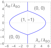
Figure 1: (Color online) Phase diagram of the Kane–Mele model determined by the entanglement spin Chern numbers (e-Ch-$\uparrow$, e-Ch-$\downarrow$) as a function of $\lambda_{\nu}$ and $\lambda_{R}$ for $t=1$ and $\lambda_{SO}=0.06$ as in Ref. PhysRevLett.95.146802. (e-Ch-$\uparrow$, e-Ch-$\downarrow$)= (1, $-1$) and (0, 0) correspond to the QSH phase and the ordinary insulator phase, respectively.

Next, we break the time-reversal symmetry by introducing the Zeeman term

$$\mathrm{H}_{Z}=-B_{0}\sum_{i}c_{i}^{\dagger}\left(\bm{n}\cdot\bm{s}\right)c_{i}$$ (6)

into the Kane–Mele model. A possible way to realize this situation is to place the honeycomb lattice on a ferromagnetic substrate.[23] Because of the time-reversal symmetry breaking, the $Z_{2}$ number becomes ill-defined, while the entanglement spin Chern number is still well-defined. In addition, the Chern number can be finite owing to the time-reversal symmetry breaking. In this paper, we choose the vector $\bm{n}$ so that its direction is perpendicular to the plane. In the following, we determine the phase diagram of the Kane–Mele model with the Zeeman term by making use of the Chern number and the entanglement spin Chern number.

Figure 2 shows the phase diagrams determined by the Chern number and the entanglement spin Chern number. In Fig. 2(a), there are phases with the Chern numbers 0, 1, and 2. In order to observe a change in the integer topological invariant, the band gap should be closed somewhere in the Brillouin zone. On the red (blue) lines in the phase diagram, the gap of the energy band closes at the K-point (K’-point). When the gap of the energy band closes at this point, the gap of the entanglement spectrum with the spin partition also closes at the same point. Typically, the Chern number changes by 1 (or $-1$) across the gap-closing line. However, there are exceptions, namely, there are lines dividing the phases with the Chern numbers 0 and 2, which will be discussed later. If the Zeeman term is turned off, the Chern number should be zero on the entire phase space, although there are several gap-closing lines in the phase space. The Zeeman term induces a split of the gap-closing line into two gap-closing lines due to the inequivalence between the K-point and K’-point, and a finite Chern number is observed in the region surrounded by the lines.

A basically identical phase diagram can be obtained by using the entanglement spin Chern numbers. The phases with the Chern numbers 1 and 2 correspond to the phases with (e-Ch-$\uparrow$, e-Ch-$\downarrow$)=(1,0) and (1,1), respectively. The phase with the Chern number 0 is somewhat special, i.e., it corresponds to (e-Ch-$\uparrow$, e-Ch-$\downarrow$)=(0,0) and (1,$-1$). That is, two phases with the same Chern number are sometimes distinguished by the entanglement Chern number. Whether the distinction between the (0,0) and (1,$-1$) states is meaningful even without time-reversal symmetry is an interesting future subject. It is worth noting that the sum rule, a rule that the Chern number is the sum of e-Ch-$\uparrow$ and e-Ch-$\downarrow$, holds in this case.

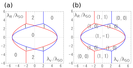
Figure 2: (Color online) Phase diagram determined by (a) Chern number and by (b) entanglement spin Chern number (e-Ch-$\uparrow$, e-Ch-$\downarrow$). In both cases $\lambda_{SO}/t=0.06$ and $B_{0}=2\lambda_{SO}$. The red (blue) line denotes the boundary of the phases where the gap of the energy band closes at the K-point (K’-point).

Let us consider the case of a large spin-orbit coupling. In this case, the energy dispersion is semimetallic i.e., the hole and electron bands overlap in the energy space.[24] However, provided the “direct gap” is always finite over the entire Brillouin zone, the Chern number is well-defined, and the phase diagram determined by the Chern number is depicted in Fig. 3. In this case, novel phases with a negative Chern number are revealed. On the red (blue) lines in the phase diagram, the gap of the energy band closes at the K-point (K’-point), as in the small spin-orbit coupling limit. On the other hand, on the purple (green) lines, the energy band closes at a point on the $\Gamma$-K ($\Gamma$-K’). On these lines, the gap of the entanglement spectrum with the spin partition also closes at a point where the energy band closes. Reflecting the three fold rotational symmetry, three Dirac cones appear in the energy dispersion of the system on the purple and green line. A single Dirac cone contributes a value of $\pm 1/2$ to the Chern number; [25] thus, the Chern number changes by 3 across the purple and green lines.

In the small spin-orbit coupling limit ($\lambda_{so}\ll t$), the purple (green) line becomes much closer to the red (blue) line. Then, the phases with a negative Chern number become invisible. This explains the existence of phase boundaries with the Chern numbers 0 and 2 in Fig. 2. Each of them is actually a pair of boundaries where one divides the phases with Chern numbers 2 and $-1$ and the other divides the phases with Chern numbers $-1$ and 0.

In the phases with a negative Chern number, the entanglement spin Chern number is undefined since the entanglement spectrum is gapless. We have shown the entanglement spectrum in Fig. 4 for the gapless case $(\lambda_{R},\lambda_{\nu})=(2.7\lambda_{SO},1.0\lambda_{SO})$. In this parameter region of negative Chern numbers, the spectrum of the entanglement Hamiltonian is always gapless. This gap-closing momentum is continuously shifted and becomes gapped at the phase boundaries specified by the green lines in Fig. 3. This phenomenon occurs for the system regardless of the value of $\lambda_{SO}$. This implies that the spin partition is not suitable for this model in the parameter region. Except in the region with a negative Chern number, there is again correspondence between the entanglement Chern number and the Chern number, i.e., the sum rule holds as in the case of $\lambda_{so}\ll t$.

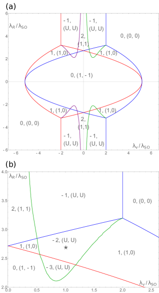
Figure 3: (Color online) (a) Phase diagram for $\lambda_{SO}=0.6t$ and $B_{0}=2\lambda_{SO}$. The Chern number and the entanglement spin Chern numbers (e-Ch-$\uparrow$, e-Ch-$\downarrow$) are indicated in each phase. (b) Magnified view of the phase diagram. The symbol “U” denotes the region where the entanglement Chern number is undefined since the entanglement spectrum is gapless (see Fig. 4).

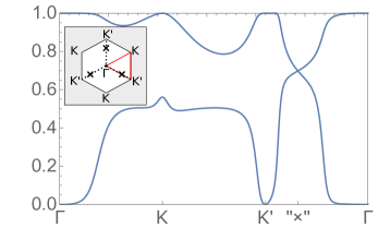
Figure 4: (Color online) Spin-up entanglement spectrum with $\lambda_{SO}=0.6t$, $B_{0}=2\lambda_{SO}$, and $(\lambda_{R},\lambda_{\nu})=(2.7\lambda_{SO},1.0\lambda_{SO})$, which correspond to the black star in Fig. 3(b). (Inset) First Brillouin zone. The gap is closed at the three points indicated by “$\times$”.

To summarize, we demonstrated that the entanglement Chern number is useful for characterizing the QSH states in the case of time-reversal invariance and the nonconservative of $s_{z}$. The results are consistent with the characterization by the $Z_{2}$ invariant. Next we found a case in which phases with the same Chern number result in a different entanglement spin Chern number even in the case of broken time-reversal symmetry, for instance, the states with (e-Ch-$\uparrow$, e-Ch-$\downarrow$)=(0, 0) and (1, $-1$) as in Fig. 2. Investigating the significance of this difference is an important future issue. Another important finding of this paper is the sum rule that the sum of the entanglement Chern numbers is equal to the original Chern number. Although this sum rule is empirical, it is ideal to have a solid theoretical explanation. The sum rule also applies to the case without time-reversal symmetry. In addition, when the time-reversal symmetry is broken, we find a finite region in the phase diagram where the entanglement spin Chern number is undefined owing to the gap closing in the entanglement spectrum, despite the fact that the gap in the energy dispersion remains finite. We should clarify whether this phenomenon is physical or is an artifact caused by an unsuitable choice of the partition. Generally, the entanglement Chern number depends on the partition. Therefore, one needs to use the most suitable partition to obtain the topological properties of a many-body ground state. It reminds us of the order parameters for describing the phase transitions, which are crucially important for choosing a suitable partition.

There are also many variants of the entanglement Chern number, i.e., we can apply not only the spin partition but also the orbital partition, the sublattice partition, the layer-by-layer partition, [26] and so on. Thus, the concept of the entanglement Chern number introduces many types of topological invariants. It is an interesting task to give intuitive understanding of the known topological phases and to explore new phases by making use of the entanglement Chern number.

References

- [1] L. Fu and C. L. Kane, Phys. Rev. B 76, 045302 (2007).
- [2] A. P. Schnyder, S. Ryu, A. Furusaki, and A. W. W. Ludwig, Phys. Rev. B 78, 195125 (2008).
- [3] X.-L. Qi, T. L. Hughes, and S.-C. Zhang, Phys. Rev. B 78, 195424 (2008).
- [4] A. Kitaev, AIP Conf. Proc. 1134, 22 (2009).
- [5] S. Ryu, A. P. Schnyder, A. Furusaki, and A. W. W. Ludwig, New J. Phys. 12, 065010 (2010).
- [6] L. Fu, Phys. Rev. Lett. 106, 106802 (2011).
- [7] T. Morimoto and A. Furusaki, Phys. Rev. B 88, 125129 (2013).
- [8] K. Shiozaki and M. Sato, Phys. Rev. B 90, 165114 (2014).
- [9] C. L. Kane and E. J. Mele, Phys. Rev. Lett. 95, 146802 (2005).
- [10] C. L. Kane and E. J. Mele, Phys. Rev. Lett. 95, 226801 (2005).
- [11] D. N. Sheng, Z. Y. Weng, L. Sheng, and F. D. M. Haldane, Phys. Rev. Lett. 97, 036808 (2006).
- [12] T. Fukui and Y. Hatsugai, Phys. Rev. B 75, 121403 (2007).
- [13] T. Fukui and Y. Hatsugai, J. Phys. Soc. Jpn. 83, 113705 (2014).
- [14] D. J. Thouless, M. Kohmoto, M. P. Nightingale, and M. den Nijs, Phys. Rev. Lett. 49, 405 (1982).
- [15] F. D. M. Haldane, Phys. Rev. Lett. 61, 2015 (1988).
- [16] Y. Hatsugai, Phys. Rev. Lett. 71, 3697 (1993).
- [17] A. Alexandradinata, T. L. Hughes, and B. A. Bernevig, Phys. Rev. B 84, 195103 (2011).
- [18] T. H. Hsieh and L. Fu, Phys. Rev. Lett. 113, 106801 (2014).
- [19] T. Fukui and Y. Hatsugai, J. Phys. Soc. Jpn. 84, 043703 (2015).
- [20] S. Ryu and Y. Hatsugai, Phys. Rev. B 73, 245115 (2006).
- [21] I. Peschel, J. Phys. A: Math. Gen. 36, L205 (2003).
- [22] T. Fukui, Y. Hatsugai, and H. Suzuki, J. Phys. Soc. Jpn. 74, 1674 (2005).
- [23] S. Rachel and M. Ezawa, Phys. Rev. B 89, 195303 (2014).
- [24] M. Laubach, J. Reuther, R. Thomale, and S. Rachel, Phys. Rev. B 90, 165136 (2014).
- [25] G. W. Semenoff, Phys. Rev. Lett. 53, 2449 (1984).
- [26] S. Predin, P. Wenk, and J. Schliemann, Phys. Rev. B 93, 115106 (2016).