Minimum Distances of the QC-LDPC Codes in IEEE 802 Communication Standards

Abstract

This work applies earlier results on Quasi-Cyclic (QC) LDPC codes to the codes specified in six separate IEEE 802 standards, specifying wireless communications from $54$ MHz to $60$ GHz. First, we examine the weight matrices specified to upper bound the codes’ minimum distance independent of block length. Next, we search for the minimum distance achieved for the parity check matrices selected at each block length. Finally, solutions to the computational challenges encountered are addressed.

I Introduction

Since the mid 2000s, LDPC codes have found a wide variety of commercial applications. Much about these codes is well understood, but rather frequently little attention is paid to the minimum (Hamming) distance between codewords. The minimum distance of a code can limit the error performance at high SNR and is important in understanding the likelihood of undetected errors. This paper presents the minimum distance of a wide variety of standardized quasi-cyclic (QC) LDPC codes.

LDPC codes are linear block codes, characterized by a sparse parity-check matrix $\mathbf{H}$. The set of codewords $\mathcal{C}$ of such a code is defined by the null-space of $\mathbf{H}$, that is $\mathcal{C}=\{\mathbf{c}\in\mathbb{F}^{n}:\mathbf{H}\,\mathbf{c}^{T}=\mathbf{0}^{T}\}$. The codewords of a block code may be divided into non-overlapping subblocks of $N$ consecutive symbols. A QC code is a linear block code having the property that applying identical circular shifts to every subblock of a codeword yields a codeword.

II Quasi-Cyclic LDPC

MacKay and Davey introduced upper bounds on the minimum distance for a class of codes that included QC-LDPC codes in [1]. Notable later work appeared in [2, 3]. Of particular relevance to this work are the upper bounds of Smarandache and Vontobel in [4].

A binary QC-LDPC code of block length $n=LN$ can be described by an $m\times n$ sparse parity-check matrix $\mathbf{H}\in\mathbb{F}_{2}^{m\times n}$, with $m=JN$, which is composed of $N\times N$ circulant submatrices. A right circulant matrix is a square matrix with each successive row right-shifted circularly one position relative to the row above. Therefore, circulant matrices can be completely described by a single row or column. As in [4, 5], we use the description corresponding to the left-most column.

In earlier works it was recognized that the set of all $N\times N$ circulant binary matrices form a commutative ring which is isomorphic to the commutative ring of polynomials with binary coefficients modulo $x^{N}-1$, i.e., $\mathbb{F}_{2}[x]/\langle{x^{N}\!-\!1}\rangle$. Specification and analysis of the QC-LDPC code can then be carried out on the much smaller polynomial parity-check matrix $\mathbf{H}(x)$ with entries from the ring, as described below.

The isomorphism between $N\times N$ binary circulant matrices and polynomial residues in the quotient ring maps a matrix to the polynomial in which the coefficients in order of increasing degree correspond to the entries in the left-most matrix column taken from top to bottom. Under this isomorphism, the $N\times N$ identity matrix maps to the multiplicative identity in the polynomial quotient ring, namely $1$. A few examples of the mapping (indicated by $\mapsto$) for $N=3$ are shown below:

$$\begin{bmatrix}1\ 0\ 0\\ 0\ 1\ 0\\ 0\ 0\ 1\end{bmatrix}\mapsto 1\quad\begin{bmatrix}0\ 0\ 1\\ 1\ 0\ 0\\ 0\ 1\ 0\end{bmatrix}\mapsto x\quad\begin{bmatrix}1\ 1\ 0\\ 0\ 1\ 1\\ 1\ 0\ 1\end{bmatrix}\mapsto 1+x^{2}.$$

Given a polynomial residue $a(x)\in\mathbb{F}_{2}[x]/\langle{x^{N}\!-\!1}\rangle$, we define its weight $\operatorname{wt}(a(x))\in\mathbb{Z}$ to be the number of nonzero coefficients. Thus, the weight $\operatorname{wt}(a(x))$ of the polynomial $a(x)$ is equal to the Hamming weight $w_{\mathrm{H}}(\mathbf{a})$ of the corresponding binary vector of coefficients $\mathbf{a}$. For a length-$L$ vector of elements in the ring, $\mathbf{a}(x)=(a_{0}(x),a_{1}(x),\ldots,a_{L-1}(x))$, we define its Hamming weight to be the sum of the weights of its components, i.e., $w_{\mathrm{H}}(\mathbf{a}(x))=\sum_{i=0}^{L-1}\operatorname{wt}(a_{i}(x))$. Throughout this work, computations implicitly shift to integer arithmetic upon taking the weight.

The parity-check matrix $\mathbf{H}$ of a binary QC-LDPC code may be presented in $J\times L$ block matrix form, such that

$${\mathbf{H}}\triangleq\left[{\begin{array}[]{ccc}{{\mathbf{H}}_{0,0}}&\cdots&{{\mathbf{H}}_{0,L-1}}\\ \vdots&\ddots&\vdots\\ {{\mathbf{H}}_{J-1,0}}&\cdots&{{\mathbf{H}}_{J-1,L-1}}\end{array}}\right],$$

where each submatrix $\mathbf{H}_{j,i}$ is an $N\times N$ binary circulant matrix. Let $h_{j,i,s}\in\mathbb{F}_{2}$ be the left-most entry in the $s$th row of the submatrix $\mathbf{H}_{j,i}$. We can then write $\mathbf{H}_{j,i}=\sum_{s=0}^{N-1}h_{j,i,s}\mathbf{I}_{s}$, where $\mathbf{I}_{s}$ is the $N\times N$ identity matrix circularly left-shifted by $s$ positions. Now, using the same convention as above for identifying matrices with polynomial residues, we can associate with $\mathbf{H}$ the polynomial parity-check matrix ${\mathbf{H}}(x)$, where ${\mathbf{H}}(x)\in\left(\mathbb{F}_{2}[x]/\langle{x^{N}\!-\!1}\rangle\right)^{J\times L}$,

$${\mathbf{H}}(x)\triangleq\left[{\begin{array}[]{ccc}{h_{0,0}(x)}&\cdots&{h_{0,L-1}(x)}\\ \vdots&\ddots&\vdots\\ {h_{J-1,0}(x)}&\cdots&{h_{J-1,L-1}(x)}\end{array}}\right],$$ (1)

and $h_{j,i}(x)\triangleq\sum_{s=0}^{N-1}{h_{j,i,s}}x^{s}$.

We will be interested in the weight of each polynomial entry of $\mathbf{H}(x)$, or, equivalently, the row or column sum of each submatrix of $\mathbf{H}$. The weight matrix of $\mathbf{H}(x)$, which is a $J\times L$ matrix of nonnegative integers, is defined as

$$\operatorname{wt}\left({{\mathbf{H}}(x)}\right)\triangleq\left[{\begin{array}[]{ccc}{\operatorname{wt}\left({h_{0,0}(x)}\right)}&\cdots&{\operatorname{wt}\left({h_{0,L-1}(x)}\right)}\\ \vdots&\ddots&\vdots\\ {\operatorname{wt}\left({h_{J-1,0}(x)}\right)}&\cdots&{\operatorname{wt}\left({h_{J-1,L-1}(x)}\right)}\\ \end{array}}\right].$$

Note that the weight matrix $\mathbf{A}\triangleq\operatorname{wt}\left({{\mathbf{H}}(x)}\right)$ is also termed the protomatrix in the context of protograph-based constructions.

We will use the shorthand notation $[L]$ to indicate the set of $L$ consecutive integers, $\left\{0,1,2,\ldots,L\!-\!1\right\}$. We let $\mathcal{S}\setminus i$ denote all the elements of $\mathcal{S}$, excluding the element $i$. We denote by $\mathbf{A}_{\mathcal{S}}$ the submatrix of $\mathbf{A}$ containing the columns indicated by the index set $\mathcal{S}$. We let $\underset{}{\operatorname{min}^{*}}$ denote the usual $\min{}$ function, but let $\underset{}{\operatorname{min}^{*}}$ exclude zero values in the argument.

We now have the background and notation to state the theorem which we use to compute the upper bounds on the minimum distance that depend on the weight matrices. This will be used extensively in the remainder of this paper.

Theorem 1 (Theorem 8 in [4]).

Let $\mathcal{C}$ be a QC code with polynomial parity-check matrix $\mathbf{H}(x)\in\left(\mathbb{F}_{2}[x]/\langle{x^{N}\!-\!1}\rangle\right)^{J\times L}$. Then the minimum distance of $\mathcal{C}$ satisfies the upper bound

$$d_{\min}(\mathcal{C})\leq\underset{\genfrac{}{}{0.0pt}{}{\mathcal{S}\subseteq[L]}{|\mathcal{S}|=J+1}}{\operatorname{min}^{*}}\sum_{i\in\mathcal{S}}{{\operatorname{perm}\left({{\mathbf{A}}_{\mathcal{S}\setminus i}}\right)}}\quad\quad(\text{in }\mathbb{Z})$$ (2)

Proof:

See [4] and [5] for proofs. ∎

III Minimum Distances by Standard

This section introduces a variety of 802-related standards and computes two upper bounds on the minimum distance of their LDPC codes. The first upper bound is (2) and is based on just the weight matrix. Thus, this bound is independent of the code’s block length and the polynomials selected for $\mathbf{H}(x)$.

The second upper bound presented is generally tighter and depends on the precise $\mathbf{H}$ selected for the standard. For this, we conduct a non-exhaustive search for small stopping sets and codewords, using Richter’s algorithm in [6] (there are others). We are unable to tighten the bounds of these searches by increasing the parameters $I$ and $T$ beyond $150$ and $15$, respectively, while using pairs of error impulses. Of course, we modified the generation of impulse locations to take advantage of QC symmetry. We denote a code’s code rate by $r$, where $r=k/n$ for $k$ information bits per block.

III-A 802.3an Ethernet

IEEE 802.3an adds a physical layer for $10$ Gigabit Ethernet over unshielded twisted pair copper cabling (10GBASE-T). A binary $(n,k)=(2048,1723)$ Reed-Solomon-based LDPC code is mandated. Its design is described by Djurdjevic et al. in [7]. It has minimum distance $14$ [8], but it is not QC .

III-B 802.11n Wireless LAN

IEEE 802.11n[9] is an amendment to the previous 802.11a/g standards for wireless local area networks in the $2.4$ and $5$ GHz microwave bands. This amendment adds a “high throughput” physical layer specification which encodes the data fields using either a binary $K=7$ convolutional code or a QC-LDPC code. Support for the convolutional code is mandatory, while the LDPC code is optional. Four code rates for each of three block length are specified. The following three tables, grouped by block length, show both upper bounds. Table I shows the largest block length codes ($n=1944$ bits, with $N=81$), Table II shows the medium block length codes ($n=1296$ bits), and Table III shows the smallest ($n=648$ bits). For rates $1/2$, $2/3$, $3/4$, and $5/6$, the $\mathbf{H}(x)$ matrices are $12\times 24$, $8\times 24$, $6\times 24$, and $4\times 24$, respectively.

III-C 802.11ad Wireless LAN at $60$ GHz

IEEE 802.11ad[10] extends the previous wireless local area network standards into the $60$ GHz (i.e.,“millimeter” wavelength) band. This standard contains a “Directional multi-gigabit” physical layer specification utilizing QC-LDPC codes to send control and data. However, a concatenated pair of Reed-Solomon block codes are also specified for an optional low-power mode. For rates $1/2$, $5/8$, $3/4$, and $13/16$, the $\mathbf{H}(x)$ matrices are $8\times 16$, $6\times 16$, $4\times 16$, $3\times 16$. In all cases, $n=672$ bits and $N=42$. Table IV summarizes the distance bounds.

TABLE I: Minimum Distance of 802.11n LDPC Codes with Large Packets

Code	U.B. of Weight Matrix	Search using Parity Check
Rate $r$	(independent of $n$)	Matrix ($n=1944$ bits)
$1/2$	$33$	$27$
$2/3$	$21$	$17$
$3/4$	$17$	$12$
$5/6$	$14$	$10$

TABLE II: Minimum Distance of 802.11n LDPC Codes with Medium-size Packets

Code	U.B. of Weight Matrix	Search using Parity Check
Rate $r$	(independent of $n$)	Matrix ($n=1296$ bits)
$1/2$	$31$	$23$
$2/3$	$17$	$14$
$3/4$	$22$	$10$
$5/6$	$17$	$9$

TABLE III: Minimum Distance of 802.11n LDPC Codes with Small Packets

Code	U.B. of Weight Matrix	Search using Parity Check
Rate $r$	(independent of $n$)	Matrix ($n=648$ bits)
$1/2$	$31$	$15$
$2/3$	$27$	$12$
$3/4$	$14$	$8$
$5/6$	$19$	$8$

TABLE IV: Minimum Distance of 802.11ad LDPC Codes

Code	U.B. of Weight Matrix	Search using Parity Check
Rate $r$	(independent of $n$)	Matrix ($n=672$ bits)
$1/2$	$19$	$17$
$5/8$	$14$	$12$
$3/4$	$13$	$9$
$13/16$	$8$	$6$

III-D 802.16e Mobile WiMAX and 802.22 Cognitive Wireless

The IEEE standard 802.16e [11], which was marketed as “WiMAX”, added mobility to the metropolitan area network (MAN) standards. Although LDPC codes were included, early WiMAX system deployments used only turbo codes. Later, the IEEE 802.22 [12] standard adopted the LDPC codes with minor changes. This standard is for cognitive wireless regional area networks (RAN) that operate in the TV bands ($54$ – $862$ MHz). Table V is organized to accommodate the many block lengths included in these two standards at each rate. For rates $1/2$, $2/3$, $3/4$, and $5/6$, the $\mathbf{H}(x)$ matrices are $12\times 24$, $8\times 24$, $6\times 24$, and $4\times 24$, respectively.

For the largest block size $n=2304$ bits, the polynomials are directly specified to create each $\mathbf{H}(x)$. For the smaller block sizes, the standard uses two techniques to create the polynomials for the reduced-sized rings based on the largest block polynomials: proportional scaling and modulo scaling of each exponent. The distances presented for 802.16e match those by Rosnes et al., in their updated paper [13].

III-E WiMedia UWB (formerly 802.15.3a)

IEEE 802.15.3a was formed to provide an ultra wideband (UWB) physical layer offering wireless speeds of 480 Mbits/s over short-ranges. The task group was officially disbanded due to the inability of parties to reach consensus between the multiband OFDM and direct sequence UWB proposals. The members of the WiMedia Alliance standardized the multiband OFDM technology using $K=7$ convolutional codes initially. This technology specifies a signal approximately $500$ MHz in bandwidth hopping across the $3.1$ – $10.6$ GHz frequency band.

Version 1.5 of the WiMedia UWB specification [14] now also specifies QC-LDPC codes. More precisely, LDPC coding is an option for all rates from $160$ to $480$ Mbits/s and is required at rates above $480$ Mbits/s. Table VI shows our findings for the four rates of this standard: $1/2$, $5/8$, $3/4$, and $4/5$. The $\mathbf{H}(x)$ matrices are quite large, at $20\times 40$, $15\times 40$, $10\times 40$, and $8\times 40$, respectively. Their size has significantly limited our ability to complete the computation of (2). The four rates mentioned here are known as the “fundamental” code rates of the standard. Each code rate has an “expanded version” with additional parity, which adds four rows and columns to $\mathbf{H}(x)$. (The expanded versions are not analyzed.)

III-F 802.15.3c millimeter WPAN

IEEE 802.15.3c has standardized a “mmWave” PHY for wireless personal area networks (WPAN) for $60$ GHz in [15]. It is intended for short-range communication and contains a variety of coding schemes. Our bounds appear in Table VII for the four rates of LDPC codes. For rates $1/2$, $3/4$, $7/8$, and $14/15$, the $\mathbf{H}(x)$ matrices are $16\times 32$, $8\times 32$, $4\times 32$, and $1\times 15$, respectively. The final one, for rate $14/15$, is unique within this work, as each entry in (1) is the summation of three cyclic permutation matrices. The entries of all other $\mathbf{H}(x)$ matrices referenced herein are cyclic permutation or zero matrices and their corresponding weight matrices are of course binary.

TABLE V: Minimum Distance of 802.16e and 802.22 LDPC Codes

Block Length	Code Rate $r$
$n$ (in bits)	$1/2$	$2/3$Aa	$2/3$B	$3/4$A	$3/4$Ba	$5/6$
$384\hbox to0.0pt{\textsuperscript{b}\hss}$	$15$	$8$	$8$	$8$	$7$	$4$
$480\hbox to0.0pt{\textsuperscript{b}\hss}$	$16$	$10$	$12$	$7$	$8$	$6$
$576$	$13$	$10$	$12$	$10$	$8$	$5$
$672$	$19$	$9$	$11$	$10$	$8$	$7$
$768$	$20$	$8$	$14$	$10$	$9$	$7$
$864$	$19$	$11$	$16$	$12$	$11$	$7$
$960$	$19$	$13$	$15$	$12$	$11$	$7$
$1056$	$21$	$10$	$15$	$13$	$9$	$7$
$1152$	$19$	$14$	$16$	$13$	$11$	$7$
$1248$	$22$	$13$	$15$	$13$	$9$	$7$
$1344$	$23$	$14$	$16$	$14$	$12$	$7$
$1440$	$27$	$13$	$17$	$12$	$10$	$7$
$1536$	$20$	$12$	$15$	$14$	$11$	$7$
$1632$	$27$	$13$	$18$	$13$	$13$	$7$
$1728$	$21$	$15$	$15$	$17$	$13$	$8$
$1824$	$19$	$15$	$15$	$13$	$12$	$8$
$1920$	$25$	$15$	$16$	$17$	$10$	$7$
$2016$	$27$	$15$	$15$	$17$	$12$	$7$
$2112$	$28$	$15$	$16$	$15$	$14$	$8$
$2208$	$23$	$15$	$20$	$18$	$13$	$8$
$2304$	$31$	$15$	$15$	$19$	$12$	$9$
U.B. of
Weight Matrix	$32$	$23$	$45$	$28$	$20$	$14$
aConfiguration appears in IEEE 802.16e, but not in 802.22.
bConfiguration appears in IEEE 802.22, but not in 802.16e.

TABLE VI: Minimum Distance of WiMedia UWB LDPC Codes

Code	U.B. of Weight Matrix	Search using Parity Check
Rate $r$	(independent of $n$)	Matrix ($n=1200$ bits)
$1/2$	$43$c	$26$
$5/8$	$35$c	$17$
$3/4$	$18$	$9$
$4/5$	$18$	$7$
cDue to complexity, matrix analysis is only $0.87\%$ and $22\%$ complete to date.

TABLE VII: Minimum Distance of 802.15.3c LDPC Codes

Code	U.B. of Weight Matrix	Search using Parity
Rate $r$	(independent of $n$)	Check Matrix
$1/2$	$36$	$18$	($n=672$ bits)
$3/4$	$16$	$10$	($n=672$ bits)
$7/8$	$16$	$6$	($n=672$ bits)
$14/15$	$6$	$6$	($n=1440$ bits)

IV Improving Computation Time

In this work and our earlier work on the AR4JA code in [5], we have found that the computation time required for (2) is frequently more than the search time of Richter’s algorithm, at the block lengths studied here (e.g., $n<4000$ bits). This is especially true for larger values of $L$. This section summarizes our efforts to speed-up the computations.

While quite similar in their definition, the matrix permanent and determinant are very different computational tasks. It is a problem well studied in combinatorics and computer algorithms, but few ready routines are published online. Also, our application frequently favors sparse matrices whose elements are often $\{0,1\}$. Without loss of generality, the focus of our implementation will be on the MATLAB computation environment while using C-programming for the permanent functions in an integrated way known as C-MEX.

IV-A Algorithms for Computing the Matrix Permanent

Clearly, computing (2) involves taking the permanent of many submatrices. By increasing the size of the permanent’s argument, we can reformulate (2) to

$$d_{\min}(\mathcal{C})\leq\underset{\genfrac{}{}{0.0pt}{}{\mathcal{S}\subseteq[L]}{|\mathcal{S}|=J+1}}{\operatorname{min}^{*}}{\operatorname{perm}\left(\begin{bmatrix}{\mathbf{A}}_{\mathcal{S}}\\ 1\ldots 1\end{bmatrix}\right)}\quad\quad(\text{in }\mathbb{Z}).$$ (3)

The summation within (2) can be viewed as a cofactor expansion of the larger matrix permanent in (3) along the bottom row, which is all-ones.

A simple method to compute the permanent is by cofactor expansion (i.e., Laplace expansion), which recursively computes the permanents of smaller and smaller matrices. This method requires about $N!N/2$ operations for a dense $N\times N$ matrix. When the matrix is sparse, as happens often in our application, the recursion can be truncated saving significant time. Our first work on this subject, in [5], relied on just such an algorithm and followed (2). We have made several advancements since then.

The first improvement was simple. Previously, for each recursive call, a new submatrix was created with the appropriate rows and columns. We realized this was wasteful and that simply keeping track of which rows and columns were removed and keeping the matrix unchanged in memory would be more efficient. This realized an overall speed-up by a factor of about three.

The best known efficient algorithm for computing general permanents is by Ryser, in[16]. It is based on the principles of inclusion-exclusion. Ryser’s method requires about $2^{N}N^{2}$ operations using standard ordering and $2^{N}N$ using an incremental Gray-coded approach. A further modification to Ryser’s algorithm by Nijenhuis and Wilf improves the computations’ speed by about a factor of two [17].

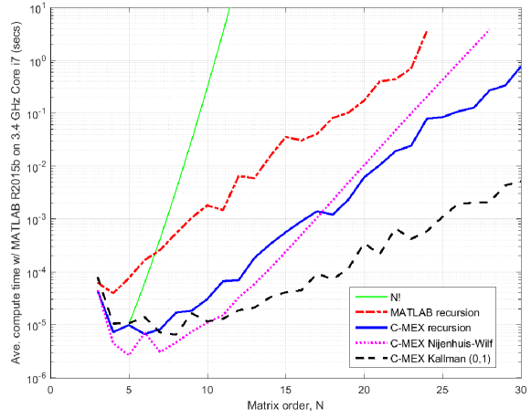
Figure 1: Average time (in secs.) to compute the permanent of $5$ random sparse $\{0,1\}$-matrices of column weight $3$ vs. matrix order $N$.

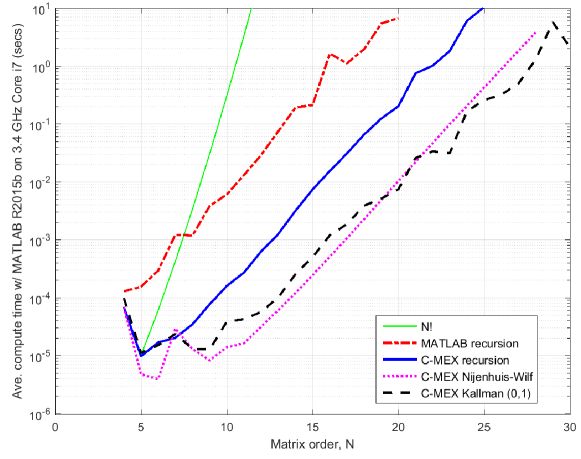
Figure 2: Average time (in secs.) to compute the permanent of $5$ random sparse $\{0,1\}$-matrices of column weight $4$ vs. matrix order $N$.

We have also found a fast permanent algorithm for $\{0,1\}$-matrices by R. Kallman in [18], which uses row operations and combinatorics to reduce the complexity substantially. It is particularly suited for sparse matrices or matrices with certain row relationships.

Since the permanent algorithms are no worse than $\operatorname{O}(N!)$ we find it worthwhile to shift from (2) to (3). Such a switch has additional gains in less C-MEX calling overhead. However, making such a switch has the effect of increasing the density of the matrix argument to the permanent function. As the computation time of our recursive algorithm is heavily dependent upon the density of the matrix, we find that it is typically no longer advantageous to use it.

The three main permanent routines mentioned are made available online at [19] and compared in Figs. 1 and 2. These results use random sparse matrices where the only constraints are the specified column weight and a non-zero permanent. While the recursive routine (solid blue) is competitive with Nijenhuis-Wilf (dotted magenta) for column weight $3$ in Fig. 1, it is much slower for column weight $4$ in Fig. 2. While the speed of Nijenhuis-Wilf and Kallman (dashed black) were comparable for column weight $4$ as shown in Fig. 2, we find that Nijenhuis-Wilf is faster for column weight $5$, not shown.

IV-B Parallel Processing

Since MATLAB has supported parallel computing for a number of years, we undertook an effort to incorporate it. There are several communication constraints between the processes. The child processes do not communicate with each other and the child processes do not easily return intermediate results to the parent process until they all complete. Thus, the simplest solution is to make a hierarchy of loops.

The lowest loop contains sufficient iterations to be a self-contained chunk of processing for a child. The middle loop utilizes the MATLAB parfor statement which works much like a for loop, but iterations are parallelized. Due to apparent overhead issues, we have set the number of iterations of this middle loop to be several times the number of hardware processors. Only upon the completion of the middle loop can intermediate results be aggregated from the children due to the constraints noted above. Thus, we prefer that the duration of the middle loop’s iterations be on the order of $30$ minutes, so that intermediate results may be monitored and saved permanently. The highest level loop then runs sufficiently long to exhaust all set combinations of (3), which may stretch to weeks in some cases. When running on the four independent processors in our 5th generation Intel Core i7 processor, we typically note a speed increase by a factor of three. These techniques would scale to even larger parallel computing environments supported by MATLAB.

Iterations proceed through an ${L\choose J+1}$ combinatorial numbering system, where each calculation is uniquely identified by the $J+1$ members of the subset $\mathcal{S}$ and the subsets are ordered lexicographically. To formulate an appropriate starting subset for each processing chunk, we implemented the $\mathrm{unrank}()$ operation which quickly translates numbering by integers to the correct subset. The $\mathrm{unrank}()$ and $\mathrm{rank}()$ routines are also made available at [19].

V Conclusions

We presented the minimum distances of a variety of QC-LDPC codes appearing in the IEEE 802-related standards. As many of the weight matrices analyzed were quite large, we have presented a simplification to the upper bound equation and computational optimizations. We are now able to compute these distance bounds at least $100$ times faster than just a few years ago.

References

- [1] D. J. C. MacKay and M. C. Davey, “Evaluation of Gallager codes for short block length and high rate applications,” in Codes, Systems and Graphical Models (Minneapolis, MN, 1999), B. Marcus and J. Rosenthal, Eds. New York: Springer-Verlag, 2000, pp. 113–130.
- [2] R. M. Tanner, D. Sridhara, A. Sridharan, T. E. Fuja, and D. J. Costello, Jr., “LDPC block and convolutional codes based on circulant matrices,” IEEE Trans. Inf. Theory, vol. 50, no. 12, pp. 2966–2984, Dec. 2004.
- [3] M. P. C. Fossorier, “Quasi-cyclic low-density parity-check codes from circulant permutation matrices,” IEEE Trans. Inf. Theory, vol. 50, no. 8, pp. 1788–1793, Aug. 2004.
- [4] R. Smarandache and P. O. Vontobel, “Quasi-cyclic LDPC codes: Influence of proto- and Tanner-graph structure on minimum Hamming distance upper bounds,” IEEE Trans. Inf. Theory, vol. 58, no. 2, pp. 585–607, Feb. 2012.
- [5] B. K. Butler and P. H. Siegel, “Bounds on the minimum distance of punctured quasi-cyclic LDPC codes,” IEEE Trans. Inf. Theory, vol. 59, no. 7, pp. 4584–4597, Jul. 2013.
- [6] G. Richter, “Finding small stopping sets in the Tanner graphs of LDPC codes,” in Proc. 4th Int. Symp. on Turbo Codes, Munich, Germany, Apr. 2006, pp. 1–5.
- [7] I. Djurdjevic, J. Xu, K. Abdel-Ghaffar, and S. Lin, “Class of low-density parity-check codes constructed based on Reed-Solomon codes with two information symbols,” IEEE Commun. Lett., vol. 7, no. 7, pp. 317–319, Jul. 2003.
- [8] S. Zhang and C. Schlegel, “Controlling the error floor in LDPC decoding,” IEEE Trans. Commun., vol. 61, no. 9, pp. 3566–3575, Sep. 2013.
- [9] IEEE Standard for Information Technology– Local and metropolitan area networks– Specific requirements– Part 11: Wireless LAN Medium Access Control (MAC) and Physical Layer (PHY) Specifications Amendment 5: Enhancements for Higher Throughput, IEEE Std. 802.11n-2009, Oct 29, 2009.
- [10] IEEE Standard for Information Technology– Local and metropolitan area networks– Specific requirements– Part 11: Wireless LAN Medium Access Control (MAC) and Physical Layer (PHY) Specifications Amendment 3: Enhancements for Very High Throughput in the 60 GHz Band, IEEE Std. 802.11ad-2012, Dec 28, 2012.
- [11] IEEE Standard for Local and metropolitan area networks– Part 16: Air Interface for Fixed and Mobile Broadband Wireless Access Systems Amendment 2: Physical and Medium Access Control Layers for Combined Fixed and Mobile Operation in Licensed Bands and Corrigendum 1, IEEE Std. 802.16e-2005 and 802.16-2004/Cor 1-2005, Feb 28 2006.
- [12] IEEE Standard for Information Technology– Local and metropolitan area networks– Specific requirements– Part 22: Cognitive Wireless RAN Medium Access Control (MAC) and Physical Layer (PHY) specifications: Policies and procedures for operation in the TV Bands, IEEE Std. 802.22-2011, July 1 2011.
- [13] E. Rosnes, Ø. Ytrehus, M. A. Ambroze, and M. Tomlinson, “Addendum to ‘An efficient algorithm to find all small-size stopping sets of low-density parity-check matrices’,” IEEE Trans. Inf. Theory, vol. 58, no. 1, pp. 164–171, Jan. 2012.
- [14] MultiBand OFDM Physical Layer Specification, WiMedia Alliance, Inc. Std. Final Deliverable 1.5, Aug 11 2009.
- [15] IEEE Standard for Information Technology– Local and metropolitan area networks– Specific requirements– Part 15.3: Amendment 2: Millimeter-wave-based Alternative Physical Layer Extension, IEEE Std. 802.15.3c-2009, Oct 12 2009.
- [16] H. J. Ryser, Combinatorial Mathematics, ser. The Carus Math. Monographs. The Mathematical Association of America, 1963, vol. 14.
- [17] A. Nijenhuis and H. S. Wilf, Combinatorial Algorithms for Computers and Calculators. New York, NY: Academic press, 1978, ch. 23.
- [18] R. Kallman, “A method for finding permanents of 0,1 matrices,” Mathematics of Computation, vol. 38, no. 157, Jan. 1982.
- [19] B. K. Butler. (2015) Files on MATLAB Central: File exchange. [Online]. Available: http://www.mathworks.com/matlabcentral/fileexchange/?term=authorid:125678