Forces for Structural Optimizations in Correlated Materials within DFT+Embedded DMFT Functional Approach

Abstract

We implemented the derivative of the free energy functional with respect to the atom displacements, so called force, within the combination of Density Functional Theory and the Embedded Dynamical Mean Field Theory. We show that in combination with the numerically exact quantum Monte Carlo (MC) impurity solver, the MC noise cancels to a great extend, so that the method can be used very efficiently for structural optimization of correlated electron materials. As an application of the method, we show how strengthening of the fluctuating moment in FeSe superconductor leads to a substantial increase of the anion height, and consequently to a very large effective mass, and also strong orbital differentiation.

I Introduction

The theoretical crystal structure prediction is one of the most fundamental challenge in condensed matter physics and material science, but it was not until 90s that computers became sufficiently powerful to allow predictions of crystal structures from first principles of very simple materials. Tsuneyuki et al. (1988); Maddox (1988) The last decade has witnessed a tremendous advance in our ability to predict crystal structures from ab-initio, mostly due to the development of efficient minimization algorithms for finding minimums in complex total energy landscape of solids Martoňák et al. (2003); Oganov and Glass (2006); Martonak et al. (2006), and because of prior development of efficient implementations of the Density Functional Theory (DFT) methods. The core of almost all these algorithms is based on the DFT stationary functional, which delivers the total energy of the solid and the forces on all atoms in the unit cell. However DFT, in its semilocal approximations such as the local density approximation (LDA) or generalized gradient approximation (GGA), fails to predict the ground state of many correlated electron materials, such as the Mott insulators and correlated metals, therefore the crystal structure predictions in such systems are severely hampered by inaccuracy of available DFT functionals.

It is well known that the DFT total energies are many times surprisingly good, even when the electronic structure is completely wrong, such as for example in high-Tc cuprates. This is because the DFT total energy functional is stationary, i.e., the first derivative of the energy with respect to electronic charge vanishes. Therefore a relatively small reorganization of the low energy valence charge density gives not too large correction to the total energy.

There are nevertheless many documented failures of LDA and GGA in predicting crystal structures of correlated materials such as in Ce metal, Pu, and transition metal oxides such as FeO. For the Hund’s metals Haule and Kotliar (2009); Yin et al. (2011), such as the iron superconductors, the pnictogen height is grosly underestimated by DFT for about 0.15Å.

To account for the correlation effects beyond semi-local approximations of DFT, more sophisticated many body methods have been developed. Among them, one of the most successful algorithms is the combination of the dynamical mean-field theory (DMFT) and DFT Anisimov et al. (1997); Lichtenstein and Katsnelson (1998); Kotliar et al. (2006), which is also based on the idea of locality of correlations, but in the case of DMFT only the locality of correlations to a given atom is explored, which is much less restrictive than locality to a point in 3D space in DFT semi-local approximations. This DFT+DMFT method has achieved great success in numerous correlated materials (for a review see Ref. Kotliar et al., 2006), but its potential for structural optimization has not been much explored. This is mostly because the majority of the implementations of this method are not implementing the DFT+DMFT functional. Instead they typically build the low energy model first, and then solve the Hubbard-like model by the DMFT method, thus losing the stationarity property, and hence the precision of the resulting total energies.

The stationary implementation of the DFT+embedded DMFT functional has been achieved recently Haule and Birol (2015), which opened the possibility of computing forces to high-enough precision for theoretical optimization of structures. The present manuscript details how this is achieved very efficiently within all electron Linearized Augmented Plane-wave (LAPW) implementation.

We will also show that in combination with the Quantum Monte Carlo (QMC) impurity solver, the forces can be converged to even higher accuracy than the free energy itself, which seems surprising at first, as only the free energy is stationary, while the forces are not. But as explained below, this is because some quantities can be more accurately computed by QMC than others. As QMC method has inherent statistical noise, such noise cancelation in computing forces is very wellcome and extremely useful for practical implementations.

The reason that the free energy is hard to compute by the exact QMC impurity solver, is that it is not possible to accurately sample the interacting part of the free energy functional, the so-called Baym-Kadanoff functional $\Phi[G]$. Essentially, $\Phi[G]$ contains the entropy of the system, which is notoriously hard to compute within the Monte Carlo methods. Frenkel (2013) An alternative approach was invented in Ref. Haule and Birol, 2015, which still requires integration over temperature for the entropy term. However, as we will show below, the force requires only the first derivative $\delta\Phi[G]/\delta G$, which is the familiar self-energy $\Sigma$, and which can be computed to very high accuracy in QMC method. It turns out that only the first derivative of the free energy functional, i.e., the force, can be so accurately implemented. To compute the free energy itself, one needs $\Phi[G]$, which is hard to compute. For the phonon spectra, which is the second derivative, one needs $\delta^{2}\Phi[G]/\delta G^{2}$, which is the two particle vertex, and is again very hard to accurately compute in practice. Therefore only the force on atoms can be computed very precisely in the DFT+embedded DMFT functional (DFT+EDMFTF) method when the exact QMC method is used as the impurity solver.

As a consequence, the frozen phonon approach is more tractable than the generalization of the density functional perturbation theory Baroni et al. (2001). Also the integration of the force will likely be the best way to calculate phase diagrams of correlated solids, as the force can be converged to much higher precision than the free energy itself.

We are aware of two prior reports on computing forces and other derivatives within DFT+DMFT method. The work of Savrasov and Kotliar Savrasov and Kotliar (2003) considered only the second derivative of the DFT+DMFT functional with respect to atom displacement, to obtain the phonon spectra. They considered only the finite wave vector ${\mathbf{q}}$, to avoid the need of differentiating the Kohn-Sham eigen-energies, which are needed for evaluating the forces. Moreover, using the Hubbard-I impurity solver, they also neglected the change of the DMFT self-energy with respect to the atom displacement ($\delta\Sigma/\delta G=\delta^{2}\Phi/\delta G^{2}$), which plays an important role in our method. The work of Leonov et. al.  Leonov et al. (2014) reported computation of forces within DFT+DMFT, however, their implementation is not based on stationary functional. The derivative of non-stationary DMFT total energy was computed, in which the two-particle vertex is needed at all frequencies, which is extremely hard to compute accurately enough by the present day impurity solvers, to be useful for the structural optimizations. Moreover, the method of Leonov et. al. Leonov et al. (2014) is a based on the two step process, where the low energy model is build first and then a Hubbard model is solved by the DMFT method. Also the influence of the DMFT correlations on the electronic charge, needed in the DFT step, is usually neglected. These two approximations are a source of inaccuracy, which is hard to overcome, even when the impurity is solved with a very high precision so that the two-particle vertex is converged within $meV$ accuracy. Hence alternative approaches are needed for practical predictions of crystal structures for correlated electron solids.

The manuscript is organized as follows: In Section II we derive the equations for the forces within DFT+Embedded DMFT functional. In part II.1 we introduce the Luttinger-Ward functional and its derivative with respect to the atom displacement, which is the well known Hellmann-Feynman force. In part II.2 we derive a basis set independent expression for the Pulay force, the additional force due to basis set discretization. In part II.3 we show how is this formula evaluated in a mixed basis set, in which the basis has both the atom-centered and origin-less functions. In part II.4 we derive Pulay forces in one such basis, namely the LAPW basis. In chapter III we apply this method to FeSe, and show how quantum Monte Carlo noise cancels to large extent when computing the force. In chapter III we also show that FeSe is positioned in the critical region where a small increase of the fluctuating moment on Fe leads to substantial increase of Se-height, and consequently also of the correlation strength. In appendix A we give details of the force evaluation within the LAPW basis set.

II Derivation of the Force within DFT+EDMFTF

The force on an atom is defined as minus the change of the total free energy when its nucleus is displaced by a small amount. The Hellmann-Feynman theorem Feynman (1939) states that this force is equal to the electrostatic force on the nucleus, but due to discretization of the problem, which involves convenient atom centered basis and atom centered projector, the actual force on an atom has additional contributions, which are usually called Pulay forces Pulay (1969).

II.1 The Luttinger-Ward approach

In ab-initio electronic structure methods, the force is computed by evaluating the analytical derivative of the total energy functional. In order to compute such derivatives, it is very convenient to use a stationary functional, in which a small change of the electron density (and the Green’s function), leaves functional invariant. Indeed, if the implementation of the functional is exact, one could evaluate the force by considering a small displacement of nuclei at fixed electron charge density (and fixed Green’s function). Namely, the total derivative of the free energy functional $\Gamma[G]$ can be split into two terms, the partial derivatives with respect to the Green’s function at fixed atomic positions, and the partial derivatives with respect to displacements at fixed Green’s function, i.e.,

$$\frac{\delta\Gamma[G]}{\delta{\mathbf{R}}_{\mu}}=\left(\frac{\partial\Gamma[G]}{\partial{\mathbf{R}}_{\mu}}\right)_{G}+\int d{\mathbf{r}}d{\mathbf{r}}^{\prime}\frac{\delta G({\mathbf{r}}{\mathbf{r}}^{\prime})}{\delta{\mathbf{R}}_{\mu}}\left(\frac{\partial\Gamma[G]}{\partial G({\mathbf{r}}{\mathbf{r}}^{\prime})}\right)_{R_{\mu}}$$ (1)

If the functional is stationary, it follows that $\left(\frac{\partial\Gamma[G]}{\partial G}\right)_{R_{\mu}}=0$, and therefore only the first term contributes, and gives so-called Hellmann-Feynman forces.

In the Green’s function approaches, such as the Dynamical Mean Field Theory, the free energy functional is best expressed by the stationary Luttinger-Ward functional, which takes the form

$$\Gamma[G]=\mathrm{Tr}\log(-G)-\mathrm{Tr}((G_{0}^{-1}-G^{-1})G)$$

$$+\Phi[G]+E_{nuclei}$$ (2)

Here $\mathrm{Tr}$ runs over spatial degrees of freedom, the spin, and when quantities are dynamic, also over Matsubara frequencies. Note that the derivative with respect to the Green’s function at constant ion position $\left(\frac{\partial\Gamma[G]}{\partial G}\right)_{R_{\mu}}$ is $G^{-1}-G_{0}^{-1}+\frac{\delta\Phi[G]}{\delta G}$, and as expected vanishes, because the system satisfies the Dyson equation $G^{-1}=G_{0}^{-1}-\frac{\delta\Phi[G]}{\delta G}$. The only term that explicitly depends on the nucleus position is contained in $G^{0}$ and $E_{nuclei}$, and the force thus becomes

$$\frac{\delta\Gamma[G]}{\delta{\mathbf{R}}_{\mu}}=-\mathrm{Tr}(G\frac{\partial G_{0}^{-1}}{\partial{\mathbf{R}}_{\mu}})+\frac{\partial E_{nuclei}}{{\mathbf{R}}_{\mu}}$$

$$=\mathrm{Tr}(\rho\frac{\partial V_{nuclei}}{\partial{\mathbf{R}}_{\mu}})+\frac{\partial E_{nuclei}}{{\mathbf{R}}_{\mu}}$$ (3)

where $G_{0}^{-1}=i\omega_{n}+\mu-T-V_{nuclei}$, and $T$, $V_{nuclei}$ are the kinetic energy operator and the potential due to nuclei, respectively. Because $V_{nuclei}$ is frequency independent, we performed a partial trace over Matsubara frequency to replace the Green’s function with the charge density in the first term $\mathrm{Tr}(G\delta V_{nuclei})=\mathrm{Tr}(\delta V_{nuclei}\frac{1}{\beta}\sum_{i\omega_{n}}G(i\omega_{n}))=\mathrm{Tr}(\rho V_{nuclei})$. The derivative in Eq. 3 then gives

$${\mathbf{F}}^{HF}=-\mathrm{Tr}(\rho\frac{\partial V_{nuclei}}{\partial{\mathbf{R}}_{\mu}})-\frac{\partial E_{nuclei}}{{\mathbf{R}}_{\mu}},$$ (4)

which is the Hellmann-Feynman force.

II.2 Forces within DFT+EDMFTF approach

The exact Baym-Kadanoff $\Phi$ functional is the sum of all skeleton Feynman diagrams, which can not be computed exactly for the solid state systems we are interested in. Within DFT+embedded DMFT functional (DFT+EDMFTF) approach, the $\Phi$ functional is approximated by the following superposition of terms

$$\Phi[G]=E_{H}[\rho]+E_{xc}[\rho]+\sum_{{\mathbf{R}}_{\mu}}\Phi^{DMFT}[G^{\mu}_{loc}]-\Phi^{DC}[\rho^{\mu}_{loc}]$$ (5)

Here the first two terms give rise to usual DFT equations, the third term adds all Feynman diagrams, local to selected set of atoms at ${\mathbf{R}}_{\mu}$. The last term subtracts the interaction, which is accounted for by both approximations. The latter is now known exactly. Haule (2015)

Notice that $\Phi^{DMFT}[G^{\mu}_{loc}]$ has the same functional form as the exact functional $\Phi^{exact}_{V_{C}}[G]$, however, to obtain $\Phi^{DMFT}$ from $\Phi^{exact}_{V_{C}}[G]$, the Green’s function $G$ is truncated to its local component $G\rightarrow G_{loc}$, and Coulomb correlation $V_{C}$ is screened, due to this truncation. Such truncation of variable of interest parallels the LDA and GGA type approximation to DFT, where $E_{XC}$ is similarly taken to be local (semilocal) to each point in 3D space, which is clearly a more restrictive approximation. The combined DFT+EDMFTF is thus a good compromise between speed and accuracy, as most of the degrees of freedom are treated on semilocal level, while the correlated orbitals are augmented by the best local approximation to a given correlated atom. Notice also that it is possible to define somewhat different functional $\Gamma$, which gives the exact local Green’s function and the exact free energy in its stationary point Chitra and Kotliar (2000), and for which the diagrammatic rules were also developed in Ref. Chitra and Kotliar, 2000. In practice, however, a successful approximation that would go beyond DMFT and would not add an exponential cost (like cluster extensions) has not been developed yet from this formalism.

To define the “locality to an atom” in Eq. 5, we need to define the DMFT projector, and in the embedded DMFT approach, this projector is chosen to be a set of atom centered functions $\ket{\phi^{\mu}_{m}}$, so that

$$G^{\mu}_{loc}({\mathbf{r}},{\mathbf{r}}^{\prime})=\sum_{mm^{\prime}}\braket{{\mathbf{r}}}{\phi^{\mu}_{m}}\braket{\phi^{\mu}_{m}}{G}{\phi^{\mu}_{m^{\prime}}}\braket{\phi^{\mu}_{m^{\prime}}}{{\mathbf{r}}^{\prime}}.$$ (6)

If these functions $\ket{\phi^{\mu}_{m}}$ form a complete basis, then DMFT method is projector independent, except that it dependents on the range of the projector (the sphere size). In practice, the solutions of the radial Schroedinger equation that correspond to the $3d$, $2p$, and $4s$ solutions, of say an Fe atom, are sufficiently separated in energy so that only $3d$ states need to be treated dynamically, while the rest of the orbitals can safely be treated statically within the exchange-correlation approximation.

The stationarity of the functional $\Gamma[G]$, when using $\Phi[G]$ of the DFT+EDMFTF (Eq. 5), gives the Dyson equation

$$G^{-1}-G_{0}^{-1}+(V_{H}+V_{xc})\delta({\mathbf{r}}-{\mathbf{r}}^{\prime})\delta(\tau-\tau^{\prime})$$

$$+\sum_{mm^{\prime},{\mathbf{R}}_{\mu}}\braket{{\mathbf{r}}}{\phi^{\mu}_{m}}\braket{\phi^{\mu}_{m}}{\Sigma-V_{DC}}{\phi^{\mu}_{m^{\prime}}}\braket{\phi^{\mu}_{m^{\prime}}}{{\mathbf{r}}^{\prime}}=0,$$ (7)

hence the electron Green’s function must satisfy

$$G^{-1}=i\omega_{n}+\mu-T-(V_{nuclei}+V_{H}+V_{xc})-$$

$$\sum_{mm^{\prime}{\mathbf{R}}_{\mu}}\ket{\phi^{\mu}_{m}}\braket{\phi^{\mu}_{m}}{\Sigma_{i\omega_{n}}-V_{DC}}{\phi^{\mu}_{m^{\prime}}}\bra{\phi^{\mu}_{m^{\prime}}}$$ (8)

and the functional $\Gamma[G]$ reaches extremum for this $G$. When inserting extremal $G$ back into $\Gamma[G]$ (Eq. 2), the value of $\Gamma$ gives the free energy of the system Abrikosov et al. (1975), which hence becomes

$$F=\mathrm{Tr}\log\left(-G\right)-\mathrm{Tr}((V_{H}+V_{xc})\rho)+E_{H}[\rho]$$

$$+E_{xc}[\rho]+E_{nuclei}-\mathrm{Tr}((\Sigma-V_{DC})\braket{\phi}{G}{\phi})$$

$$+\sum_{{\mathbf{R}}_{\mu}}\Phi^{DMFT}[G^{\mu}_{loc}]-\Phi^{DC}[\rho^{\mu}_{loc}]+\mu N$$ (9)

Notice that $(\braket{\phi}{G}{\phi})_{mm^{\prime}}$ are the matrix elements of the local Green’s function $\braket{\phi_{m}^{\mu}}{G}{\phi_{m^{\prime}}^{\mu}}$.

In the all-electron calculations of the free energy, the spatial degrees of freedom are expanded in terms of a mixed basis set, which includes atom centered basis functions, therefore the Hellmann-Feynman force is very different from the derivative of the implemented free energy Eq. 9. It is therefore essential to find the analytic derivative of the actually implemented free energy Eq. 9. This is derived below. We will concentrate on the valence electron contribution, as the core contribution within DFT+EDMFTF is the same as in DFT.

To evaluate the logarithm of the Green’s function in Eq. 9, we first solve the following frequency dependent eigenvalue-problem

$$\bra{\psi_{j{\mathbf{k}}\omega_{n}}}(T+V_{nuclei}+V_{H}+V_{xc}+\sum_{mm^{\prime}{\mathbf{R}}_{\mu}}\ket{\phi^{\mu}_{m}}\braket{\phi^{\mu}_{m}}{\Sigma_{i\omega_{n}}-V_{DC}}{\phi^{\mu}_{m^{\prime}}}\bra{\phi^{\mu}_{m^{\prime}}})\ket{\psi_{i{\mathbf{k}}\omega_{n}}}=\delta_{ij}\;\varepsilon_{{\mathbf{k}}\omega_{n},i}$$ (10)

so that the Green’s function is simply given by

$$\braket{\psi_{j{\mathbf{k}}\omega_{n}}}{G}{\psi_{i{\mathbf{k}}\omega_{n}}}=\frac{\delta_{ij}}{i\omega_{n}+\mu-\varepsilon_{{\mathbf{k}}\omega_{n},i}}$$ (11)

and the free energy is evaluated by

$$F=-\mathrm{Tr}\log\left(-i\omega_{n}-\mu+\varepsilon_{{\mathbf{k}}\omega_{n}}\right)-\mathrm{Tr}((V_{H}+V_{xc})\rho)$$

$$+E_{H}[\rho]+E_{xc}[\rho]+E_{nuclei}-\mathrm{Tr}((\Sigma-V_{DC})\braket{\phi}{G}{\phi})$$

$$+\sum_{{\mathbf{R}}_{\mu}}\Phi^{DMFT}[G^{\mu}_{loc}]-\Phi^{DC}[\rho^{\mu}_{loc}]+\mu N$$ (12)

This is the actual expression implemented in DFT+EDMFTF code. To get the force on an atom, we need to consider a small variation of this energy when moving an atom at position ${\mathbf{R}}_{\mu}$

$$\delta F=\mathrm{Tr}\left(\frac{\delta\varepsilon_{{\mathbf{k}}\omega_{n}}-\delta\mu}{i\omega_{n}+\mu-\varepsilon_{{\mathbf{k}}\omega_{n}}}\right)-\mathrm{Tr}(\rho(\delta V_{H}+\delta V_{xc}))$$

$$-\mathrm{Tr}(G_{loc}(\delta\Sigma-\delta V_{DC}))+\delta E_{nuclei}+N\delta\mu$$ (13)

where we used the fact that

$$\delta(E_{H}+E_{xc})=\mathrm{Tr}((V_{H}+V_{xc})\delta\rho)$$ (14)

$$\sum_{{\mathbf{R}}_{\mu}}\delta\Phi^{DMFT}[G^{\mu}_{loc}]+\delta\Phi^{DC}[\rho^{\mu}_{loc}]=\mathrm{Tr}((\Sigma-V_{DC})\delta G_{loc})$$

and, as we work at constant electron density, $\delta N=0$. Inserting the Hellmann-Feynman forces Eq. 4, we arrive at

$$\delta F=\mathrm{Tr}\left(\frac{\delta\varepsilon_{{\mathbf{k}}\omega_{n}}}{i\omega_{n}+\mu-\varepsilon_{{\mathbf{k}}\omega_{n}}}\right)-\mathrm{Tr}(\rho\;\delta V_{KS})$$

$$-\mathrm{Tr}(G_{loc}(\delta\Sigma-\delta V_{DC}))-\sum_{\mu}{\mathbf{F}}^{HF}_{\mu}\delta{\mathbf{R}}_{\mu}$$ (15)

where $V_{KS}=V_{H}+V_{xc}+V_{nuclei}$.

Finally, we define the Pulay force on an atom ${\mathbf{F}}^{Puly}$ as the addition to the Hellmann-Feynman force (due to the basis set in which the functional is implemented) $\delta F=-\sum_{\mu}({\mathbf{F}}^{HF}_{\mu}+{\mathbf{F}}^{Puly}_{\mu})\delta{\mathbf{R}}_{\mu}$. From Eq. 15 it follows that the Pulay forces are

$${\mathbf{F}}^{Puly}_{\mu} = -\mathrm{Tr}\left(\frac{1}{i\omega_{n}+\mu-\varepsilon_{{\mathbf{k}}\omega_{n}}}\frac{\delta\varepsilon_{{\mathbf{k}}\omega_{n}}}{d{\mathbf{R}}_{\mu}}\right)$$ (16)

$$+ \mathrm{Tr}\left(\rho\frac{\delta V_{KS}}{\delta{\mathbf{R}}_{\mu}}\right)+\mathrm{Tr}\left(G_{loc}\frac{\delta\Sigma-\delta V_{DC}}{\delta{\mathbf{R}}_{\mu}}\right)$$

This equation is still completely general expression for the force within the DFT+EDMFTF, irrespectively of the basis set employed.

II.3 Pulay forces expressed in a mixed basis set

To proceed, we need to choose a basis to express the electron Green’s function. We will here denote it by $\ket{\chi_{\mathbf{K}}}$, (as we have in mind LAPW basis set) but the details of the basis are not important here, so this derivation is relevant for any mixed basis set.

The DMFT eigenvectors $\ket{\psi_{i{\mathbf{k}}\omega_{n}}}$ are than expanded in the chosen basis in the usual way

$$\ket{\psi_{i{\mathbf{k}}\omega_{n}}}=\sum_{{\mathbf{K}}}\ket{\chi_{{\mathbf{K}}}}A^{R}_{{\mathbf{K}}i}$$ (17)

$$\bra{\psi_{i{\mathbf{k}}\omega_{n}}}=\sum_{{\mathbf{K}}}A^{L}_{i{\mathbf{K}}}\bra{\chi_{{\mathbf{K}}}}$$ (18)

Note that the eigenvectors $\ket{\psi_{i{\mathbf{k}}\omega_{n}}}$ are momentum and frequency dependent, hence $A^{R}_{{\mathbf{K}}i}$ also inherit this momentum and frequency dependence, i.e., $A^{R}_{{\mathbf{K}}i}=A^{R}_{{\mathbf{K}}i}({\mathbf{k}},\omega_{n})$. Note also that the eigenvalue problem is not Hermitian, therefore we need to distinguish between the right and the left eigenvectors. Using expansion Eqs. 17 and 18, the DMFT eigenvalue problem Eq. 10 reads

$$\sum_{{\mathbf{K}}{\mathbf{K}}^{\prime}}A^{L}_{j{\mathbf{K}}^{\prime}}\left[H^{0}_{{\mathbf{K}}^{\prime}{\mathbf{K}}}+V_{{\mathbf{K}}^{\prime}{\mathbf{K}}}\right]A^{R}_{{\mathbf{K}}i}=\delta_{ij}\;\varepsilon_{{\mathbf{k}}\omega_{n},i}$$ (19)

where

$$H^{0}_{{\mathbf{K}}^{\prime}{\mathbf{K}}}=\braket{\chi_{{\mathbf{K}}^{\prime}}}{T+V_{nuclei}+V_{H}+V_{xc}}{\chi_{\mathbf{K}}}$$ (20)

$$V_{{\mathbf{K}}^{\prime}{\mathbf{K}}}=\sum_{mm^{\prime}{\mathbf{R}}_{\mu}}\braket{\chi_{{\mathbf{K}}^{\prime}}}{\phi^{\mu}_{m}}\braket{\phi^{\mu}_{m}}{\Sigma-V_{DC}}{\phi^{\mu}_{m^{\prime}}}\braket{\phi^{\mu}_{m^{\prime}}}{\chi_{\mathbf{K}}}$$

Here $H^{0}$ stands for the DFT part of the Hamiltonian, and $V$ for the additional DMFT contributions.

The eigenvectors are orthogonalized in the usual way

$$\sum_{{\mathbf{K}}{\mathbf{K}}^{\prime}}A^{L}_{i{\mathbf{K}}^{\prime}}O_{{\mathbf{K}}^{\prime}{\mathbf{K}}}A^{R}_{{\mathbf{K}}j}=\delta_{ij}$$

where $O_{{\mathbf{K}}^{\prime}{\mathbf{K}}}=\braket{\chi_{{\mathbf{K}}^{\prime}}}{\chi_{{\mathbf{K}}}}$ is the overlap matrix, hence the eigenvalue problem Eq. 19 can be cast in the following form

$$\sum_{{\mathbf{K}}}\left[H^{0}_{{\mathbf{K}}^{\prime}{\mathbf{K}}}+V_{{\mathbf{K}}^{\prime}{\mathbf{K}}}\right]A^{R}_{{\mathbf{K}}i}=\sum_{{\mathbf{K}}}O_{{\mathbf{K}}^{\prime}{\mathbf{K}}}A^{R}_{{\mathbf{K}}i}\;\varepsilon_{{\mathbf{k}}\omega_{n},i}$$ (21)

or in short notation

$$[H^{0}+V]A^{R}=OA^{R}\varepsilon.$$

Eq. 21 is enforced for any position of atoms ${\mathbf{R}}_{\mu}$, hence its variation vanishes. We thus have

$$[(\delta H^{0})+(\delta V)]A^{R}+[H^{0}+V]\delta A^{R}$$

$$=(\delta O)A^{R}\varepsilon+O(\delta A^{R})\varepsilon+OA^{R}\delta\varepsilon$$ (22)

and multiplying with $A^{L}$ we get

$$A^{L}[(\delta H^{0})+(\delta V)]A^{R}+A^{L}[H^{0}+V]\delta A^{R}$$

$$=A^{L}(\delta O)A^{R}\varepsilon+A^{L}O(\delta A^{R})\varepsilon+\delta\varepsilon$$ (23)

We also use the fact that $A^{L}[H^{0}+V]=\varepsilon A^{L}O$ to obtain

$$\delta\varepsilon=A^{L}[(\delta H^{0})+(\delta V)]A^{R}-A^{L}(\delta O)A^{R}\varepsilon$$

$$+\varepsilon A^{L}O(\delta A^{R})-A^{L}O(\delta A^{R})\varepsilon$$ (24)

In Eq. 16 we only need the diagonal variation of the eigenvalues $(\delta\varepsilon)_{ii}$, for which the last two terms cancel because $\varepsilon$ is diagonal matrix, hence $\varepsilon_{i}(A^{L}O(\delta A^{R}))_{ii}-(A^{L}O(\delta A^{R})_{ii}\varepsilon_{i}=0$. We thus obtain

$$(\delta\varepsilon_{{\mathbf{k}}\omega_{n}})_{ii}=\sum_{{\mathbf{K}}{\mathbf{K}}^{\prime}}A^{L}_{i{\mathbf{K}}^{\prime}}[\delta H^{0}_{{\mathbf{K}}^{\prime}{\mathbf{K}}}+\delta V_{{\mathbf{K}}^{\prime}{\mathbf{K}}}]A^{R}_{{\mathbf{K}}i}$$

$$-A^{L}_{i{\mathbf{K}}^{\prime}}\,\delta O_{{\mathbf{K}}^{\prime}{\mathbf{K}}}\,A^{R}_{{\mathbf{K}}i}\,\varepsilon_{{\mathbf{k}}\omega_{n},i}$$ (25)

This is a dynamic generalization of the DFT expression, derived in Ref. Yu et al., 1991.

Next we split the DMFT eigenvectors into the static (Kohn-Sham) part, and the frequency dependent part

$$A^{R}_{{\mathbf{K}}i}=\sum_{j}A^{0}_{{\mathbf{K}}j}(B^{R}_{\omega_{n}})_{ji}$$ (26)

$$A^{L}_{i{\mathbf{K}}}=\sum_{j}(B^{L}_{\omega_{n}})_{ij}A^{0\,\dagger}_{j{\mathbf{K}}}$$ (27)

or short $A^{R}=A^{0}B^{R}_{\omega_{n}}$ and $A^{L}=B^{L}_{\omega_{n}}A^{0\dagger}$. Here $A^{0}$ satisfies the Kohn-Sham eigenvalue problem $A^{0\dagger}H^{0}A^{0}=\varepsilon^{0}$.

In terms of the above defined quantities Eq. 16 takes the form

$${\mathbf{F}}^{Puly}_{\mu}=-\mathrm{Tr}\left(G^{d}B_{\omega_{n}}^{L}\left[A^{0\dagger}\left(\frac{\delta H^{0}}{\delta{\mathbf{R}}_{\mu}}+\frac{\delta V}{\delta{\mathbf{R}}_{\mu}}\right)A^{0}B_{\omega_{n}}^{R}-A^{0\dagger}\frac{\delta O}{\delta{\mathbf{R}}_{\mu}}A^{0}B_{\omega_{n}}^{R}\varepsilon_{{\mathbf{k}}\omega_{n}}\right]\right)+\mathrm{Tr}\left(\rho\frac{\delta V_{KS}}{\delta{\mathbf{R}}_{\mu}}\right)+\mathrm{Tr}\left(G_{loc}\frac{\delta\Sigma-\delta V_{DC}}{\delta{\mathbf{R}}_{\mu}}\right)$$ (28)

where we denoted

$$G^{d}=\frac{1}{i\omega_{n}+\mu-\varepsilon_{{\mathbf{k}}\omega_{n}}},$$

and $G^{d}$ is the Green’s function in diagonal representation. Next we define the following DMFT density matrices

$$\widetilde{\rho} \equiv \frac{1}{\beta}\sum_{i\omega_{n}}B^{R}_{\omega_{n}}\frac{1}{i\omega_{n}+\mu-\varepsilon_{{\mathbf{k}}\omega_{n}}}B^{L}_{\omega_{n}}$$ (29)

$$\widetilde{(\rho\varepsilon)} \equiv \frac{1}{\beta}\sum_{i\omega_{n}}B^{R}_{\omega_{n}}\frac{\varepsilon_{{\mathbf{k}}\omega_{n}}}{i\omega_{n}+\mu-\varepsilon_{{\mathbf{k}}\omega_{n}}}B^{L}_{\omega_{n}}$$ (30)

which are the usual DMFT density matrices, but here written in the Kohn-Sham basis. Note that the density matrix $\widetilde{\rho}$ can also be expressed by $\widetilde{\rho}_{ij}=\braket{\psi^{0}_{i}}{\rho}{\psi^{0}_{j}}$ where $\ket{\psi^{0}}$ are Kohn-Sham eigenvectors of $H^{0}$ and $\rho$ is the self-consistent charge density of DFT+EDMFTF method. We also recognize the Green’s functions written in the $\ket{\chi_{\mathbf{K}}}$ basis

$$\bar{G}_{{\mathbf{K}}{\mathbf{K}}^{\prime}}=(A^{0}B_{\omega_{n}}^{R}\frac{1}{i\omega_{n}+\mu-\varepsilon_{{\mathbf{k}}\omega_{n}}}B_{\omega_{n}}^{L}A^{0\dagger})_{{\mathbf{K}}{\mathbf{K}}^{\prime}}$$ (31)

The overline here is used to stress that the Green’s function is expressed in the basis of $\ket{\chi_{\mathbf{K}}}$ (rather than in real space). This allows us to simplify

$${\mathbf{F}}^{Puly}_{\mu}=-\mathrm{Tr}\left(\widetilde{\rho}A^{0\dagger}\frac{\delta H^{0}}{d{\mathbf{R}}_{\mu}}A^{0}-\widetilde{(\rho\varepsilon)}A^{0\dagger}\frac{\delta O}{\delta{\mathbf{R}}_{\mu}}A^{0}\right)+\mathrm{Tr}\left(\rho\frac{\delta V_{KS}}{\delta{\mathbf{R}}_{\mu}}\right)-\mathrm{Tr}\left(\bar{G}\frac{\delta V}{\delta{\mathbf{R}}_{\mu}}\right)+\mathrm{Tr}\left(G_{loc}\frac{\delta\Sigma-\delta V_{DC}}{\delta{\mathbf{R}}_{\mu}}\right)$$ (32)

We next simplify the interacting part (the third term above), which contains interaction $V$ (defined by Eq. 20):

$$\mathrm{Tr}\left(\bar{G}\delta V\right)$$

$$=\frac{1}{\beta}\sum_{\begin{subarray}{c}i\omega,m^{\prime}m\\ {\mathbf{K}}{\mathbf{K}}^{\prime}\end{subarray}}\bar{G}_{{\mathbf{K}}{\mathbf{K}}^{\prime}}\delta\left(\braket{\chi_{{\mathbf{K}}^{\prime}}}{\phi_{m^{\prime}}}(\Sigma-V_{DC})_{m^{\prime}m}\braket{\phi_{m}}{\chi_{{\mathbf{K}}}}\right)$$

$$=\frac{1}{\beta}\sum_{\begin{subarray}{c}i\omega_{n},m^{\prime}m\\ {\mathbf{K}}{\mathbf{K}}^{\prime}\end{subarray}}\bar{G}_{{\mathbf{K}}{\mathbf{K}}^{\prime}}(\Sigma-V_{DC})_{m^{\prime}m}\delta\left(\braket{\chi_{{\mathbf{K}}^{\prime}}}{\phi_{m^{\prime}}}\braket{\phi_{m}}{\chi_{{\mathbf{K}}}}\right)$$

$$+\mathrm{Tr}\left(G_{loc}(\delta\Sigma-\delta V_{DC})\right)$$ (33)

where we used the fact that

$$(G_{loc})_{mm^{\prime}}=\sum_{{\mathbf{K}}{\mathbf{K}}^{\prime}}\braket{\phi_{m}}{\chi_{{\mathbf{K}}}}\bar{G}_{{\mathbf{K}}{\mathbf{K}}^{\prime}}\braket{\chi_{{\mathbf{K}}^{\prime}}}{\phi_{m^{\prime}}}$$

Finally, the Pulay forces become

$${\mathbf{F}}^{Puly}_{\mu}=-\mathrm{Tr}\left(\widetilde{\rho}A^{0\dagger}\frac{\delta H^{0}}{\delta{\mathbf{R}}_{\mu}}A^{0}-\widetilde{(\rho\varepsilon)}A^{0\dagger}\frac{\delta O}{\delta{\mathbf{R}}_{\mu}}A^{0}\right)+\mathrm{Tr}\left(\rho\;\frac{\delta V_{KS}}{\delta{\mathbf{R}}_{\mu}}\right)$$

$$-\frac{1}{\beta}\sum_{i\omega_{n}}\sum_{{\mathbf{K}}{\mathbf{K}}^{\prime},m^{\prime}m}\bar{G}_{{\mathbf{K}}{\mathbf{K}}^{\prime}}(\Sigma-V_{DC})_{m^{\prime}m}\frac{\delta\left(\braket{\chi_{{\mathbf{K}}^{\prime}}}{\phi_{m^{\prime}}}\braket{\phi_{m}}{\chi_{{\mathbf{K}}}}\right)}{\delta{\mathbf{R}}_{\mu}}$$ (34)

This is still a basis independent expression of the Pulay force, as we abstain discussing specifics of a given basis set, but we nevertheless managed to avoid the expensive frequency summations in all but the last term. To perform the expensive ${\mathbf{K}}$ and frequency summation in the last term, we need to determine the derivative of the projector, which depends on the basis set and the choice of a projector.

II.4 Pulay forces within LAPW basis and quasi atomic orbital projector

Within the LAPW method Slater (1937); Andersen (1975) the interstitial space is spanned by the plane waves $\widetilde{\chi}_{\mathbf{K}}$, while inside the muffin-tin spheres, the plane waves are augmented and expanded as a linear superposition of the atom-centered solutions of the Schroedinger equation. We name these augmented functions $\chi_{\mathbf{K}}$, and inside muffin-tin spheres we express them in the atom centered coordinate system with the proper phase factor $\chi_{{\mathbf{K}}}({\mathbf{r}})=e^{i({\mathbf{K}}+{\mathbf{k}}){\mathbf{R}}_{\mu}}\bar{\chi}_{\mathbf{K}}({\mathbf{r}}-{\mathbf{R}}_{\mu})$. For convenience of the derivation, we chose $\bar{\chi}_{\mathbf{K}}$ to be the basis function in the muffin-tin sphere, but without the phase factor. The matrix elements of the Hamiltonian are then computed by an integral of the form

$$\braket{\chi_{{\mathbf{K}}^{\prime}}}{V}{\chi_{{\mathbf{K}}}}=\int_{int}d^{3}r\widetilde{\chi}^{*}_{{\mathbf{K}}^{\prime}}({\mathbf{r}})V({\mathbf{r}})\widetilde{\chi}_{\mathbf{K}}({\mathbf{r}})+\sum_{\mu}e^{i({\mathbf{K}}-{\mathbf{K}}^{\prime}){\mathbf{R}}_{\mu}}\int_{MT_{\mu}}d^{3}r\bar{\chi}^{*}_{{\mathbf{K}}^{\prime}}({\mathbf{r}})V({\mathbf{r}}+{\mathbf{R}}_{\mu})\bar{\chi}_{\mathbf{K}}({\mathbf{r}})$$ (35)

The first term runs over interstitial space between muffin-tin (MT) spheres, while the second term is the MT part. We are looking for a change when we move a single atom $\mu$ at ${\mathbf{R}}_{\mu}$ for a small amount ($\delta{\mathbf{R}}_{\mu}$). The plane-wave functions $\widetilde{\chi}_{\mathbf{K}}$ do not change, while the augmented $\bar{\chi}_{{\mathbf{K}}}$ in the second integral move with the atom. In addition, because the nucleus moves, the charge gets deformed and the potential changes for an unknown amount $\delta V$. We will keep track of this change, but we know that it must eventually cancel out, since we are taking derivative of a stationary functional. This is the crucial advantage of a stationary functional, as otherwise one would need to evaluate terms like $(\delta\Sigma/\delta G){\delta G}=(\delta^{2}\Phi/\delta G^{2}){\delta G}$, i.e., the two particle vertex $\delta^{2}\Phi/\delta G^{2}$ would need to be computed at all frequencies, which is numerically extremely hard to achieve using existing impurity solvers.

Finally, we will make the usual approximation Yu et al. (1991); Kohler et al. (1996) that the LAPW basis functions $\bar{\chi}_{\mathbf{K}}({\mathbf{r}}-{\mathbf{R}}_{\mu})$ rigidly shift with the displacement of the atom, but do not deform, in the so-called frozen radial augmentation function approximation.

Under this assumptions, the change of a matrix elements is

$$\frac{\delta\braket{\chi_{{\mathbf{K}}^{\prime}}}{V}{\chi_{\mathbf{K}}}}{\delta{\mathbf{R}}_{\mu}}=\braket{\chi_{{\mathbf{K}}^{\prime}}}{\frac{\delta V}{\delta{\mathbf{R}}_{\mu}}}{\chi_{{\mathbf{K}}}}-\oint_{MT_{\mu}}d{\mathbf{S}}\,\widetilde{\chi}^{*}_{{\mathbf{K}}^{\prime}}\,V\,\widetilde{\chi}_{\mathbf{K}}+i({\mathbf{K}}-{\mathbf{K}}^{\prime})\braket{\chi_{{\mathbf{K}}^{\prime}}}{V}{\chi_{\mathbf{K}}}_{MT_{\mu}}+\braket{\chi_{{\mathbf{K}}^{\prime}}}{\nabla V}{\chi_{{\mathbf{K}}}}_{MT_{\mu}}$$ (36)

The first term is due to the movement of the nucleus, and associated change of the charge and the potential. The integral in this term is extended over the entire space. The second term is due to the change of the integration area for the interstitial component, and extends over the surface of the moving MT-sphere. The third term is due to the phase factor in Eq. 35, and the last term arises due to the fact that the potential in the sphere is expressed in the moving coordinate system centered on the moving atom. We used here a short notation $\braket{\chi_{{\mathbf{K}}^{\prime}}}{V}{\chi_{{\mathbf{K}}}}_{MT_{\mu}}$ for the integral over the MT-sphere $\int_{MT_{\mu}}d^{3}r\chi^{*}_{{\mathbf{K}}^{\prime}}V\chi_{\mathbf{K}}$.

The matrix element for the kinetic energy operator, which takes the form

$$\braket{\chi_{{\mathbf{K}}^{\prime}}}{T}{\chi_{{\mathbf{K}}}}=\int_{int}d^{3}r(\nabla\widetilde{\chi}^{*}_{{\mathbf{K}}^{\prime}}({\mathbf{r}}))\cdot(\nabla\widetilde{\chi}_{\mathbf{K}}({\mathbf{r}}))+\sum_{\mu}e^{i({\mathbf{K}}-{\mathbf{K}}^{\prime}){\mathbf{R}}_{\mu}}\int_{MT_{\mu}}d^{3}r\nabla(\bar{\chi}^{*}_{{\mathbf{K}}^{\prime}}({\mathbf{r}}))\cdot\nabla(\bar{\chi}_{\mathbf{K}}({\mathbf{r}}))$$ (37)

does not have the first and the last term of Eq. 36, as the form of $\nabla\cdot\nabla$ is originless, and hence does not change with the movement of the nucleus, nor with the movement of the coordinate system. We thus have

$$\frac{\delta\braket{\chi_{{\mathbf{K}}^{\prime}}}{T}{\chi_{\mathbf{K}}}}{\delta{\mathbf{R}}_{\mu}}=-\oint_{MT_{\mu}}d{\mathbf{S}}\,\widetilde{\chi}^{*}_{{\mathbf{K}}^{\prime}}\,T\,\widetilde{\chi}_{\mathbf{K}}$$

$$+i({\mathbf{K}}-{\mathbf{K}}^{\prime})\braket{\chi_{{\mathbf{K}}^{\prime}}}{T}{\chi_{\mathbf{K}}}_{MT_{\mu}}$$ (38)

Similarly, the overlap has only the following two terms

$$\frac{\delta\braket{\chi_{{\mathbf{K}}^{\prime}}}{\chi_{\mathbf{K}}}}{\delta{\mathbf{R}}_{\mu}}=-\oint_{MT_{\mu}}d{\mathbf{S}}\,\widetilde{\chi}^{*}_{{\mathbf{K}}^{\prime}}\widetilde{\chi}_{\mathbf{K}}$$

$$+i({\mathbf{K}}-{\mathbf{K}}^{\prime})\braket{\chi_{{\mathbf{K}}^{\prime}}}{\chi_{\mathbf{K}}}_{MT_{\mu}}$$ (39)

Finally, we also need the derivative of the DMFT projector $\delta\left(\braket{\chi_{{\mathbf{K}}^{\prime}}}{\phi_{m^{\prime}}}\braket{\phi_{m}}{\chi_{{\mathbf{K}}}}\right)/\delta{\mathbf{R}}_{\mu}$. This can be looked at as a matrix element computed in Eq. 35, where the potential is replaced by $V\rightarrow\braket{{\mathbf{r}}^{\prime}}{\phi_{m^{\prime}}}\braket{\phi_{m}}{{\mathbf{r}}}=\phi_{m^{\prime}}({\mathbf{r}}^{\prime})\phi_{m}^{*}({\mathbf{r}})$. In our implementation of embedded-DMFT, the projector vanishes outside the MT-sphere, hence the integrals over the interstitials vanishes. Inside the MT-sphere, we rigidly shift the localized functions $\phi_{m}({\mathbf{r}})$ and not deform them, hence $\delta(\phi_{m^{\prime}}\phi^{*}_{m})=-\nabla(\phi_{m^{\prime}}\phi^{*}_{m})$, so that the first and the last term in Eq. 36 cancel, hence we have

$$\frac{\delta\left(\braket{\chi_{{\mathbf{K}}^{\prime}}}{\phi_{m^{\prime}}}\braket{\phi_{m}}{\chi_{{\mathbf{K}}}}\right)}{\delta{\mathbf{R}}_{\mu}}=i({\mathbf{K}}-{\mathbf{K}}^{\prime})\braket{\chi_{{\mathbf{K}}^{\prime}}}{\phi_{m^{\prime}}}\braket{\phi_{m}}{\chi_{{\mathbf{K}}}}$$ (40)

Note that Wannier orbitals do not rigidly shift with the atom, as they explicitly depend on the electron charge, hence the derivative of the projector in the Wannier basis is not so simple. Hence the Pulay forces within the DFT+DMFT approach, implemented in Wannier basis, is much more complicated than derived here.

Finally, let us note that the equivalent expressions for the derivatives Eqs. 36, 38, and  39 were derived by Soler & Williams Soler and Williams (1989), as well as by Rici, Singh, and Krakauer Yu et al. (1991). The two formalisms were shown to be equivalent in Ref. Soler and Williams, 1993.

Next we use the Gauss theorem to simplify

$$\braket{\chi_{{\mathbf{K}}^{\prime}}}{\nabla V}{\chi_{\mathbf{K}}}_{MT}=\oint_{MT}d{\mathbf{S}}\,\chi^{*}_{{\mathbf{K}}^{\prime}}\,V\,\chi_{\mathbf{K}}$$

$$-\int_{MT}d^{3}rV\,\nabla(\chi^{*}_{{\mathbf{K}}^{\prime}}\chi_{\mathbf{K}})$$ (41)

and derive a convenient expression for the change of the static part of the Hamiltonian $H^{0}=T+V_{KS}$:

$$\frac{\delta H^{0}_{{\mathbf{K}}^{\prime}{\mathbf{K}}}}{\delta{\mathbf{R}}_{\mu}}=\braket{\chi_{{\mathbf{K}}^{\prime}}}{\frac{\delta V_{KS}}{\delta{\mathbf{R}}_{\mu}}}{\chi_{{\mathbf{K}}}}+i({\mathbf{K}}-{\mathbf{K}}^{\prime})\braket{\chi_{{\mathbf{K}}^{\prime}}}{H^{0}}{\chi_{\mathbf{K}}}_{MT_{\mu}}-\oint_{MT_{\mu}}d{\mathbf{S}}\,(\nabla\widetilde{\chi}^{*}_{{\mathbf{K}}^{\prime}})\cdot(\nabla\widetilde{\chi}_{\mathbf{K}})$$

$$-\int_{MT}d^{3}rV_{KS}\,\nabla(\chi^{*}_{{\mathbf{K}}^{\prime}}\chi_{\mathbf{K}})+\oint_{MT}d{\mathbf{S}}\,\left[\chi^{*}_{{\mathbf{K}}^{\prime}}\,V_{KS}\,\chi_{\mathbf{K}}-\widetilde{\chi}^{*}_{{\mathbf{K}}^{\prime}}\,V_{KS}\,\widetilde{\chi}_{\mathbf{K}}\right]$$ (42)

where

$$\braket{\chi_{{\mathbf{K}}^{\prime}}}{H^{0}}{\chi_{{\mathbf{K}}}}_{MT_{\mu}}=\braket{\chi_{{\mathbf{K}}^{\prime}}}{T+V_{KS}}{\chi_{{\mathbf{K}}}}_{MT_{\mu}}$$

$$=\int_{MT_{\mu}}d^{3}r(\nabla\chi^{*}_{{\mathbf{K}}^{\prime}})\cdot(\nabla\chi_{{\mathbf{K}}})+\braket{\chi_{{\mathbf{K}}^{\prime}}}{V_{KS}}{\chi_{{\mathbf{K}}}}_{MT_{\mu}}$$

$$=\braket{\chi_{{\mathbf{K}}^{\prime}}}{-\nabla^{2}+V_{KS}}{\chi_{\mathbf{K}}}_{MT_{\mu}}+\oint_{MT_{\mu}}d{\mathbf{S}}\,\chi^{*}_{{\mathbf{K}}^{\prime}}\nabla\chi_{\mathbf{K}}$$ (43)

The last term in Eq. 42 vanishes if the basis functions $\chi_{{\mathbf{k}}}$ are continuos across the MT-sphere. The continuity is enforced in both LAPW and APW+lo method. There is however always a very small discontinuity, which is due to the fact hat the harmonics expansion contains finite number of spheric harmonics. We usually take large enough cutoff $l\approx 10$ so that this term is around two orders of magnitude smaller than the rest of the terms, and can therefore be safely ignored.

Next, we insert Eq. 42 into Eq. 34, and evaluate term by term. The first term $\mathrm{Tr}(\widetilde{\rho}A^{0\dagger}\delta V_{KS}A^{0})$ can be greatly simplified

$$\mathrm{Tr}\left(\widetilde{\rho}A^{0\dagger}\frac{\delta V_{KS}}{\delta{\mathbf{R}}_{\mu}}A^{0}\right)=\sum_{ij{\mathbf{K}}{\mathbf{K}}^{\prime}}\widetilde{\rho}_{ij}A^{0\dagger}_{j{\mathbf{K}}^{\prime}}\braket{\chi_{{\mathbf{K}}^{\prime}}}{\frac{\delta V_{KS}}{\delta{\mathbf{R}}_{\mu}}}{\chi_{\mathbf{K}}}A^{0}_{{\mathbf{K}}j}$$

$$=\sum_{ij}\braket{\psi_{i}^{0}}{\rho}{\psi_{j}^{0}}\braket{\psi_{j}^{0}}{\frac{\delta V_{KS}}{\delta{\mathbf{R}}_{\mu}}}{\psi_{i}^{0}}=\mathrm{Tr}\left(\rho\frac{\delta V_{KS}}{\delta{\mathbf{R}}_{\mu}}\right)$$ (44)

This is because the Kohn-Sham solution $\ket{\psi_{i}^{0}}=\sum_{\mathbf{K}}\ket{\chi_{\mathbf{K}}}A^{0}_{{\mathbf{K}}i}$ and $\widetilde{\rho}=\braket{\psi^{0}}{\rho}{\psi^{0}}$ is the density matrix expressed in the Kohn-Sham basis. Clearly this term cancels a term in Eq. 34, as expected for stationary functional, hence the real change of the Kohn-Sham potential due to movement of nucleus (and not due to movement of the basis attached to the sphere) is not needed in the force calculation.

Next we simplify the forth term of Eq. 42 when inserted into Eq. 34. We have

$$\mathrm{Tr}\left(\widetilde{\rho}A^{0\dagger}\int V_{KS}\nabla(\chi^{*}\chi)A^{0}\right)$$

$$=\sum_{{\mathbf{K}}{\mathbf{K}}^{\prime},ij}\widetilde{\rho}_{ij}A^{0\dagger}_{i{\mathbf{K}}^{\prime}}\int d^{3}rV_{KS}({\mathbf{r}})\nabla(\chi^{*}_{{\mathbf{K}}^{\prime}}\chi_{\mathbf{K}})A^{0}_{{\mathbf{K}}j}=$$

$$\int d^{3}rV_{KS}({\mathbf{r}})\sum_{ij}\braket{\psi^{0}_{i}}{\rho}{\psi^{0}_{j}}\nabla(\psi^{0*}_{j}({\mathbf{r}})\psi^{0}_{i}({\mathbf{r}}))$$

$$=\int d^{3}rV_{KS}({\mathbf{r}})\nabla\rho({\mathbf{r}})=\mathrm{Tr}(V_{KS}\nabla\rho)$$ (45)

Finally, we also simplify the last term in the Pulay forces Eq. 34, which comes from the DMFT dynamic corrections

$${\mathbf{F}}^{dynam}\equiv-\frac{1}{\beta}\sum_{i\omega_{n}}\sum_{{\mathbf{K}}{\mathbf{K}}^{\prime},m^{\prime}m}\bar{G}_{{\mathbf{K}}{\mathbf{K}}^{\prime}}(\Sigma-V_{DC})_{m^{\prime}m}\frac{\delta\left(\braket{\chi_{{\mathbf{K}}^{\prime}}}{\phi_{m^{\prime}}}\braket{\phi_{m}}{\chi_{{\mathbf{K}}}}\right)}{\delta{\mathbf{R}}_{\mu}}$$ (46)

Using Eq. 40 and the fact that the Green’s function Eq. 31 can also be expressed in the smaller Kohn-Sham basis

$$\tilde{G}_{ij}=\left(B_{\omega_{n}}^{R}\frac{1}{i\omega_{n}+\mu-\varepsilon_{{\mathbf{k}}\omega_{n}}}B_{\omega_{n}}^{L}\right)_{ij}=\braket{\psi^{0}_{i}}{G}{\psi^{0}_{j}}$$ (47)

so that $\bar{G}_{{\mathbf{K}}^{\prime}{\mathbf{K}}}=(A^{0}\tilde{G}A^{0\dagger})_{{\mathbf{K}}^{\prime}{\mathbf{K}}}$ we arrive at

$${\mathbf{F}}^{dynam}=-\frac{1}{\beta}\sum_{i\omega_{n}}\sum_{ij,m^{\prime}m}\tilde{G}_{ij}(\Sigma-V_{DC})_{m^{\prime}m}\times$$ (48)

$$\times\sum_{{\mathbf{K}}{\mathbf{K}}^{\prime}}A^{0\dagger}_{j{\mathbf{K}}^{\prime}}i({\mathbf{K}}-{\mathbf{K}}^{\prime})\braket{\chi_{{\mathbf{K}}^{\prime}}}{\phi_{m^{\prime}}}\braket{\phi_{m}}{\chi_{{\mathbf{K}}}}A^{0}_{{\mathbf{K}}i}$$

The projector, which expresses the DMFT Green’s function in the Kohn-Sham basis, is given by

$${\cal U}_{mi}=\sum_{{\mathbf{K}}}\braket{\phi_{m}}{\chi_{{\mathbf{K}}}}A^{0}_{{\mathbf{K}}i}$$ (49)

from which the DMFT local Green’s function is usually computed

$$G_{loc}(i\omega_{n})\equiv{\cal U}\tilde{G}(i\omega){\cal U}^{\dagger}$$ (50)

Note that here $G_{loc}$ is expressed in the DMFT orbital basis $mm^{\prime}$.

We can compute a vector version of the DMFT projector, which is given by

$$\vec{{{\cal U}}}_{mi}=\sum_{{\mathbf{K}}}\braket{\phi_{m}}{\chi_{{\mathbf{K}}}}{\mathbf{K}}A^{0}_{{\mathbf{K}}i}$$ (51)

to simplify the dynamic force

$${\mathbf{F}}^{dynam}=-\frac{i}{\beta}\sum_{i\omega_{n}}\sum_{ij,m^{\prime}m}(\Sigma_{m^{\prime}m}(i\omega_{n})-V^{DC}_{m^{\prime}m})(\vec{{\cal U}}_{mi}\tilde{G}_{ij}(i\omega_{n}){\cal U}^{\dagger}_{jm^{\prime}}-{\cal U}_{mi}\tilde{G}_{ij}(i\omega_{n})\vec{{\cal U}}^{\dagger}_{jm^{\prime}})$$ (52)

The first term has the form $\mathrm{Tr}(\Sigma(i\omega_{n})\vec{{\cal U}}\tilde{G}(i\omega_{n}){\cal U}^{\dagger})$ and if we replace $i\omega_{n}\rightarrow-i\omega_{n}$ we get $\mathrm{Tr}(\Sigma(i\omega_{n}){\cal U}\tilde{G}(i\omega_{n})\vec{{\cal U}}^{\dagger})^{*}$, which is complex conjugated second term. The resulting force ${\mathbf{F}}^{dynamic}$ is therefore a real number.

We normally compute the local Green’s function by Eq. 50, but it is convenient to compute also the following vector version of the local Green’s function

$$\vec{G}_{loc}(i\omega_{n})\equiv\vec{{\cal U}}\tilde{G}(i\omega){\cal U}^{\dagger}$$ (53)

from which the dynamic force can be computed very efficiently

$${\mathbf{F}}^{dynam}=2\textrm{Im}\mathrm{Tr}((\Sigma(i\omega_{n})-V^{DC})\vec{G}_{loc}(i\omega_{n})).$$ (54)

This calculation needs only a summation over Matsubara frequencies and over correlated orbitals, and hence ${\mathbf{F}}^{dynamic}$ can be computed almost as fast as the DMFT density matrix.

Finally we insert the rest of the terms in Eqs. 42 and 39 into Eq. 34, to obtain the complete expression of the Pulay forces for the valence states within LAPW basis

$${\mathbf{F}}^{Puly}_{\mu}=-\sum_{{\mathbf{K}}{\mathbf{K}}^{\prime}ij}\widetilde{\rho}_{ij}A^{0\dagger}_{j{\mathbf{K}}^{\prime}}\,i({\mathbf{K}}-{\mathbf{K}}^{\prime})\braket{\chi_{{\mathbf{K}}^{\prime}}}{H^{0}}{\chi_{\mathbf{K}}}_{MT_{\mu}}A^{0}_{{\mathbf{K}}i}$$ (55)

$$+\sum_{{\mathbf{K}}{\mathbf{K}}^{\prime}ij}\widetilde{(\rho\varepsilon)}_{ij}A^{0\dagger}_{j{\mathbf{K}}^{\prime}}i({\mathbf{K}}-{\mathbf{K}}^{\prime})\braket{\chi_{{\mathbf{K}}^{\prime}}}{\chi_{\mathbf{K}}}_{MT_{\mu}}A^{0}_{{\mathbf{K}}i}$$ (56)

$$+\sum_{{\mathbf{K}}{\mathbf{K}}^{\prime}ij}\left[\widetilde{\rho}_{ij}({\mathbf{k}}+{\mathbf{K}})\cdot({\mathbf{k}}+{\mathbf{K}}^{\prime})-\widetilde{(\rho\varepsilon)}_{ij}\right]A^{0\dagger}_{j{\mathbf{K}}^{\prime}}A^{0}_{{\mathbf{K}}i}\oint_{MT_{\mu}}d{\mathbf{S}}\,\widetilde{\chi}^{*}_{{\mathbf{K}}^{\prime}}\widetilde{\chi}_{\mathbf{K}}$$ (57)

$$+\mathrm{Tr}(V_{KS}\nabla\rho)+2\textrm{Im}\mathrm{Tr}((\Sigma-V^{DC})\vec{G}_{loc})$$ (58)

The first two terms contain the MT-integrals and their similar structure but opposite sign shows how they would cancel in the absence of the $i({\mathbf{K}}-{\mathbf{K}}^{\prime})$ term. The latter arises from the fact that the basis inside MT-sphere is moved with the nucleus. Eq. 57 contains so-called MT-surface terms which arise due to discontinuity of the second derivative across MT-sphere Yu et al. (1991), and finally the last term is due to the fact that the DMFT projector moves with the displacement of the nucleus.

The DMFT density matrices $\widetilde{\rho}$ and $\widetilde{(\rho\varepsilon)}$ are computed by careful summation over the Matsubara points. Once these density matrices are computed in the Kohn-Sham basis, we can diagonalize them

$$\widetilde{\rho}\equiv{\cal B}\;w\;{\cal B}^{\dagger}$$ (59)

$$\widetilde{(\rho\varepsilon)}\equiv\overline{{\cal B}}\;(w\varepsilon)\;\overline{{\cal B}}^{\dagger}$$ (60)

and obtain two sets of eigenvectors ${\cal B}$, $\overline{{\cal B}}$ and the corresponding eigenvalues $w_{i}$ and $(w\varepsilon)_{i}$, respectively. Then we can insert the diagonal form for the density matrices into Eqs. 55, 56, 57 to obtain Pulay forces in a compact form

$${\mathbf{F}}^{Puly}_{\mu}=-\sum_{{\mathbf{K}}{\mathbf{K}}^{\prime}i}w_{i}A^{\dagger}_{i{\mathbf{K}}^{\prime}}\,i({\mathbf{K}}-{\mathbf{K}}^{\prime})\braket{\chi_{{\mathbf{K}}^{\prime}}}{H^{0}}{\chi_{\mathbf{K}}}_{MT_{\mu}}A_{{\mathbf{K}}i}+\sum_{{\mathbf{K}}{\mathbf{K}}^{\prime}i}(w\varepsilon)_{i}\overline{A}^{\dagger}_{j{\mathbf{K}}^{\prime}}i({\mathbf{K}}-{\mathbf{K}}^{\prime})\braket{\chi_{{\mathbf{K}}^{\prime}}}{\chi_{\mathbf{K}}}_{MT_{\mu}}\overline{A}_{{\mathbf{K}}i}$$ (61)

$$+\sum_{{\mathbf{K}}{\mathbf{K}}^{\prime}i}\left[w_{i}A^{\dagger}_{i{\mathbf{K}}^{\prime}}({\mathbf{k}}+{\mathbf{K}}^{\prime})\cdot({\mathbf{k}}+{\mathbf{K}})A_{{\mathbf{K}}i}-(w\varepsilon)_{i}\overline{A}^{\dagger}_{i{\mathbf{K}}^{\prime}}\overline{A}_{{\mathbf{K}}i}\right]\oint_{MT_{\mu}}d{\mathbf{S}}\,\widetilde{\chi}^{*}_{{\mathbf{K}}^{\prime}}\widetilde{\chi}_{\mathbf{K}}$$ (62)

$$+\mathrm{Tr}(V_{KS}\nabla\rho)+2\textrm{Im}\mathrm{Tr}((\Sigma-V^{DC})\vec{G}_{loc})$$ (63)

Here we used the modified eigenvectors

$$A=A^{0}{\cal B}$$ (64)

$$\overline{A}=A^{0}\overline{{\cal B}}$$ (65)

The resulting Eqs. 61,62,63 have now very similar form as the DFT Pulay forces within LAPW method Kohler et al. (1996), except in DFT $A$ and $\overline{A}$ are both equal to the KS-eigenvectors, and $w_{i}$’s are fermi functions $f_{i}$ and $(w\varepsilon)_{i}$ are fermi function times KS-eigenvalues ($f_{i}\varepsilon_{i}$). The last term in Eq. 63 bares some resemblance to the LDA+U force Tran et al. (2008), but is different due to dynamic nature of $\Sigma$ and $G_{loc}$. The algorithm to evaluate these terms is given in appendix A.

III Results

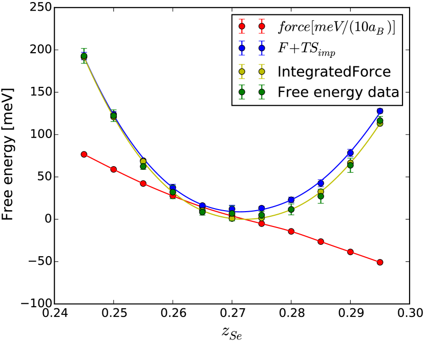
Figure 1: (Color online): Force on Se atom when displaced in $z$-direction, and the corresponding change of the free energy. The free energy is calculated from the functional Eq. 9, and is compared to integrated force. We show both the free energy and $F+TS_{imp}$. The latter is directly computed in our method, while the former requires additional integration over the temperature. The quantum Monte Carlo noise is approximately one order of magnitude smaller when computing energy from the force than computing it directly from the functional.

We tested the method on several transition metal oxides, pnictides and chalchogenides.  In this section, we show result for FeSe, one of the most studied member of iron superconductor family, which has attracted tremendous attention recently. We use the implementation of DFT+EDMFT of Ref. Haule et al., 2010, which is based on Wien2k Blaha et al. (2001). The value of Coulomb $U$ is fixed at $5\,$eV Kutepov et al. (2010), and we use the nominal double-counting Haule (2015).

Bulk FeSe crystalizes in tetragonal P4/nmm structure (No. 129). It is superconducting below 10 K under ambient pressure Hsu et al. (2008), and the superconducting T_c is increases to 37 K under pressure Medvedev et al. (2009); Margadonna et al. (2009). By substitution of Se by small amounts of Te, T_c can also be increased to 15 K Yeh, Kuo-Wei et al. (2008); Sales et al. (2009), and by intercalation with spacer layers, T_c can also be boosted to over 40 K Lu et al. (2014).

First we test the implementation of forces within DFT+EDMFTF by computing force on Se, located at Wickoff position 2c $(1/4,1/4,z_{Se})$ versus the Se height $z_{Se}$. As shown in Fig. 1 the force is almost linear around the equilibrium position, and its integral matches quite well (within the statistical noise) to the free energy of the system. Note that there is always some systematic error due to frozen radial augmentation approximation, i.e., in computing the force we do not differentiate the solutions of the radial Schroedinger equation $u_{l}$. In Fig. 1 we show both the free energy, and the free energy without the impurity entropy. The latter quantity is computed directly from the Green’s function, while the former needs additional integration over temperature Haule and Birol (2015). Notice that the error-bars in computing the force are significantly smaller than the error-bars on the free energy.

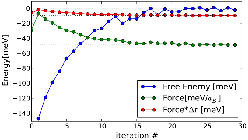
Figure 2: (Color online): The convergence of the free energy $F+TS_{imp}$ and force with the number of DMFT iterations. The last seven steps are converged, but display typical Monte Carlo noise, which is more severe in free energy than in computing force. When the force is multiplied with the displacement from equilibrium $\Delta$r, to recover the units of energy, the noise is more than one order of magnitude smaller than the corresponding noise of the free energy. The data corresponds to $z_{Se}=0.25$. For clarity we subtracted a constant from both the energy and the force.

To make this point more clear, we show in Fig. 2 the free energy and the force from our simulation. We count as a start of the new iteration whenever the DMFT self-energy is updated, but note that we perform approximately 10 charge self-consistent steps for each self-energy update, so that the charge is practically converged at each DMFT iteration. As is clear from Fig. 2, the Monte Carlo noise in computing the free energy, of the order of a few meV, is present even when the free energy is converged, and only better statistics in the QMC solver can reduce this noise. The calculated force, measured in meV per atomic unit, has almost factor of five smaller noise than the free energy. Finally, when we convert the force to units of meV (by multiplying with the distance from the equilibrium) this contribution to free energy has almost no visible noise (approximately two orders of magnitude smaller noise than the free energy itself). Even when we integrate the force, to obtain the free energy, the error remains almost one order of magnitude smaller, compared to the error in direct calculation of the energy. We believe that this is because the $\Phi$-functional is much more challenging to compute precisely within Monte Carlo Haule and Birol (2015), while the derivative of $\Phi$ is the self-energy, which is very precisely sampled by the Monte Carlo method.

Many authors suggested that Se-height plays an important role in determining superconducting T_c in Fe-superconductors Mizuguchi et al. (2010). Theoretical studies of correlations in iron superconductors showed, that the level of correlation strength is strongly coupled to the anion-height Yin et al. (2011), as the higher anion position increases the distance between Fe and the anion, thereby reducing the Fe-anion hybridization. As a consequence, the strength of the local magnetic moment is increased and correlations are increased. This is clear from the substitution of Se by larger Te, which increases the anion heigh, and as a consequence, the correlation strength is increased significantly. Yin et al. (2011). Note that this effect was recently also confirmed experimentally. Ieki et al. (2014)

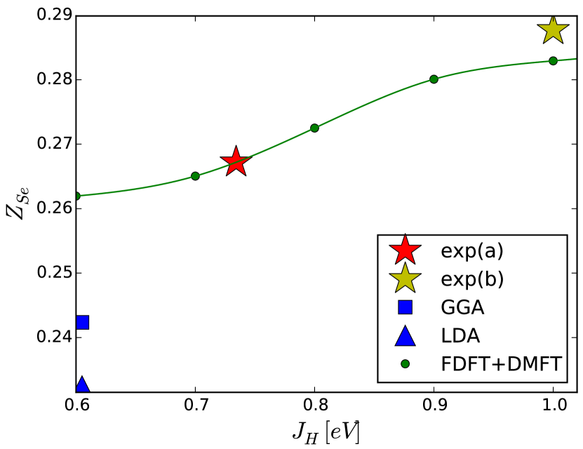
Figure 3: (Color online): The optimized $z$ position of Se atom for different values of Hund’s coupling $J_{H}$. The experimental values exp(a) and exp(b) correspond to X-ray measurements of Ref. McQueen et al., 2009 and Ref. Kumar et al., 2010, respectively.

As discussed above, previous theoretical studies and the experiments suggest that the increased anion height leads to larger fluctuating moment, but in the previous theoretical studies the crystal structures of various Fe superconductors was taken from experiment, and was not theoretically optimized. To estimate the electron-phonon coupling in FeSe within DFT+DMFT, the coupling between the crystal structure and electronic structure was analyzed in Ref. Mandal et al., 2014, using only the total energy of the system, as we did not have implementation of forces, and structural optimization was very time consuming.

To establish that the size of the fluctuating moment and anion height are internally consistently predicted by the theory, one should see that larger fluctuating moment must lead to increased anion heigh, as otherwise cancelation effect would occur and possibly significantly reduce or even reverse the effect, previously predicted by theory Yin et al. (2011).

Here we calculate the optimized Se height as a function of Hund’s rule coupling $J_{H}$, which has a strong effect on strengthening the fluctuating moment. Haule and Kotliar (2009) It is natural to expect that an increased fluctuating moment will reduce tendency to bind, and hence increase anion heigh. It is however interesting to see in Fig. 4 that this effect is strongest at exactly the physically most relevant value of $J_{H}\approx 0.8\,$eV Kutepov et al. (2010). At larger $J_{H}>0.9\,$eV and smaller $J_{H}<0.7\,$eV, the curve tends to saturate. We thus see that FeSe is situated at exactly the critical position, where small change of its correlation strength, or fluctuating moment, changes its properties dramatically. It is tempting to correlate this with experimental findings that pressure and intercalation has a dramatic effect of its T_c.

We notice that both LDA and GGA significantly underestimate the anion-height. We mark two X-ray measurements on powder samples in Fig. 4, which lead to somewhat different value for $z_{Se}$. This discrepancy will likely be resolved by measurements on a single crystal of FeSe. DMFT agrees better with Ref. McQueen et al., 2009, as $J_{H}$ of 0.75 eV is quite close to best estimates of its value in iron superconductors Kutepov et al. (2010). The Se-heigh from Ref. Kumar et al., 2010 is somewhat outside the values suggested by the present theory. We note that Ref. McQueen et al., 2009 considered wider range on angles in the fit, hence it likely lead to more precise value for $Z_{Se}$ than in Ref. Kumar et al., 2010.

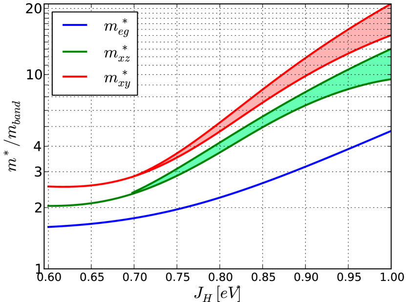
Figure 4: (Color online): Mass enhancement of different orbitals versus Hund’s coupling $J_{H}$, when $z_{Se}$ is optimized theoretically. Note logarithmic scale for mass.

While the change of $z_{Se}$ from 0.265 at $J_{H}=0.7\,$eV to $z_{Se}=0.28$ at $J_{H}=0.9\,$eV might seem small, we show below that it has dramatic consequence for the strength of correlations on Fe atom. Previous studies of the 5-band Hubbard model Haule and Kotliar (2009) have established that for fixed crystal structure, the increase of the Hund’s rule coupling increases effective mass and the correlation strength. But here we show that by considering the feedback effect of the magnetic moment on the crystal structure, this effect appears to be even stronger. In Fig. 4 we show the strengthening of the effective mass, as compared to LDA, for different orbitals versus Hund’s coupling. Note that for larger $J_{H}$, we do not give a single number, but rather a range of values for $m^{*}$. This is because our calculation is performed at fixed temperature $T\approx 50\,$K, at which the metallic state becomes increasingly incoherent with increased $J_{H}$. In such incoherent metal, different extrapolations of the numerical data can lead to different estimates of the mass, hence we mark a range. The size of the spread can also be used as a measure of incoherency, namely, as the orbital is more incoherent, its precision for mass estimation decreases. Experimentally, at $50\,$K the measured band dispersion should be more consistent with the lowest estimation of the mass, while at even lower temperature in the Fermi liquid regime, the mass should increase and should be more consistent with the highest estimates.

Notice that the plot is logarithmic, hence Hund’s coupling increases mass exponentially for all orbitals. Notice also that the mass differentiation is also increased exponentially, for example at $J_{H}=0.9$ the $xy$ orbital has over 50% larger mass than $xz/yz$ orbital, while at $J_{H}=0.7$, the $xy$ orbital is only 20% more massive than $xz/yz$. Hence, Hund’s coupling not just increases correlations, but rather makes differentiation between orbitals larger.

This is one of the central elements of the physics of Hund’s metals Haule and Kotliar (2009); Yin et al. (2012), in which spin-spin Kondo coupling turns ferromagnetic and therefore slows down spin fluctuations, thereby increasing the effective mass of quasiparticles, while the charge fluctuations remain very fast, and hence charge is not blocked, unlike in the Hubbard or t-J model. Due to coupling of the spin and orbital through Kondo physics, the system becomes Fermi liquid at zero temperature. Yin et al. (2012) This physics is thus very different from the Hubbard physics.

Here we used rotationally invariant Slater form of the Coulomb interaction, where Slater integrals are related to $J_{H}$ by $F^{2}=8.6154J_{H}$ and $F^{4}=5.3846J_{H}$. Note that the same value of $J_{H}$, using simpler Kanamori parametrization of the Coulomb repulsion, leads to even larger mass enhancements.

Note also that we do not see spin-frozen ground state, or proximity to a quantum critical points, as found in some model studies Werner et al. (2008), whenever we use rotationally invariant form of the Hund’s coupling. When we use the density-density interaction only, which is not rotationally invariant, we do however find spin-freezing and incoherent metal, in which coherence is not restored with decreasing temperature. The latter seems to be a property of certain forms of Coulomb interactions, which do not explicitly obey rotational invariance, and the reason behind deserves further study.

IV Conclusions and Discussion

In this manuscript we derived forces on atoms within ab-initio approach termed DFT+Embedded DMFT functional. This method combines the DFT with the DMFT such that it embeds the DMFT Feynman diagrams directly in real space to the DFT real space functional. The resulting functional is stationary, as we ensure that the projector $P=\sum_{\alpha\beta}\ket{\phi_{\alpha}}\bra{\phi_{\alpha}}\otimes\ket{\phi_{\beta}}\bra{\phi_{\beta}}$ is independent of the electronic charge density, so that $\delta P/\delta G=0$. This property of the projector ensures that the variation of functional $\delta\Gamma[G]$ vanishes when the usual Dyson Eq. 7 is satisfied. Note that when Wannier functions are used for projector, then $\delta P/\delta G$ does not vanish, and hence the variation of the functional $\Gamma[G]$ does not lead to a usual form of the Dyson equation Eq. 7. More complicated Dyson equation would than need to be used.

The derivative of the stationary functional with respect to atomic displacement was derived analytically, and we showed that the Pulay force contains only simple terms, which appear due to our choice of atom centered basis. We show explicitly that quantities, which are numerically difficult to evaluate, cancel out. In particular, the two particle vertex function, which appears due to variation of the self-energy $\delta\Sigma/\delta G$, cancels out. Moreover, the $\Phi[G]$ functional, which is needed for free energy evaluation, is not needed for computing forces. The resulting forces on atoms can thus be very efficiently computed, and we implemented them in LAPW basis. We showed that even though quantum Monte Carlo leads to considerable noise in evaluating the free energy (noise of the order of a $meV$) the force contains less noise (of the order of $0.2~{}meV/a.u.$), hence this precision of the force allows one to efficiently optimize crystal structures.

We optimized the crystal structure of FeSe for different values of Hund’s coupling, and we showed that stronger fluctuating moment leads to increase of the Se-height. The latter has dramatic impact on the correlations in this system, as the mass increases exponentially with the strength of the Hund’s coupling. At the same time, the orbital differentiation also increases exponentially with $J_{H}$. This is the central property of the Hund’s metals Haule and Kotliar (2009).

The new formula for evaluating forces on all atoms in the unit cell within DFT+DMFT formalism thus has a great potential for both the structural predictions, as well as prediction of phase diagrams of correlated materials at finite temperature, which are known to have very complex phase diagrams.

V Acknowledgement

This work was supported by Simons foundation under project ”Many Electron Problem”, and by NSF-DMR 1405303. This research used resources of the Oak Ridge Leadership Computing Facility at the Oak Ridge National Laboratory, which is supported by the Office of Science of the US Department of Energy under Contract No. DE-AC05-00OR22725. We are grateful to Gabriel Kotliar for numerous fruitful discussions, and for carefully reading the manuscript.

Appendix A Details of the force evaluation in the LAPW basis set

First we set up the notation for the LAPW basis set. The basis functions in the interstitials are

$$\chi_{{\mathbf{k}}+{\mathbf{K}}}({\mathbf{r}})=\frac{1}{\sqrt{V}}e^{i({\mathbf{k}}+{\mathbf{K}}){\mathbf{r}}}$$ (66)

and in the MT-spheres they take the form

$$\chi_{{\mathbf{k}}+{\mathbf{K}}}({\mathbf{r}})=\sum_{lm,\mu}(a_{lm\mu{\mathbf{K}}}u_{l}\left(|{\mathbf{r}}-{\mathbf{r}}_{\mu}|)+b_{lm\mu{\mathbf{K}}}\dot{u}_{l}(|{\mathbf{r}}-{\mathbf{r}}_{\mu}|)\right)Y_{lm}(R_{\mu}({\mathbf{r}}-{\mathbf{r}}_{\mu}))$$ (67)

$$\chi_{\nu}({\mathbf{r}})=\sum_{m^{\prime}\mu^{\prime}}(a^{lo}_{\nu,m^{\prime}\mu^{\prime}}u_{l}(|{\mathbf{r}}-{\mathbf{r}}_{\mu^{\prime}}|)+b^{lo}_{\nu,m^{\prime}\mu^{\prime}}\dot{u}_{l}(|{\mathbf{r}}-{\mathbf{r}}_{\mu^{\prime}}|)+c^{lo}_{\nu,m^{\prime}\mu^{\prime}}u^{LO}_{l}(|{\mathbf{r}}-{\mathbf{r}}_{\mu^{\prime}}|))Y^{*}_{lm^{\prime}}(R_{\mu^{\prime}}{\mathbf{r}})$$ (68)

where Eq. 67 stands for augmented plane wave functions, which are matched with the plane wave Eq. 66 at the MT-sphere boundary, and Eq. 68 are additional local orbitals, which vanish at the MT-boundary and hence do not need augmentation in the interstitials. The index $\nu$ of the local orbitals comprises several indices $\nu=(i_{sort},l,j_{lo},\mu,m)$, where $i_{sort}$ and $\mu$ are the type of atom and the index of atom of a give $i_{sort}$ type, respectively. $j_{lo}$ is the successive index of the local orbital (as several local orbitals per atom are possible), and $l,m$ is the index of the spherical harmonics. Notice that in Eq. 68 we sum over all equivalent atoms $\mu^{\prime}$ in the unit cell, hence a given local orbital has a contribution in each equivalent atom and for each $m$ of a given $l$. The precise form of the coefficients appearing in these two equations is

$$a_{lm\mu{\mathbf{K}}}\equiv\bar{a}^{{\mathbf{k}}+{\mathbf{K}}}_{l}\;\frac{4\pi i^{l}S^{2}}{\sqrt{V}}e^{i({\mathbf{k}}+{\mathbf{K}}){\mathbf{r}}_{\mu}}Y^{*}_{lm}(R_{\mu}({\mathbf{k}}+{\mathbf{K}}))$$

$$b_{lm\mu{\mathbf{K}}}\equiv\bar{b}^{{\mathbf{k}}+{\mathbf{K}}}_{l}\;\frac{4\pi i^{l}S^{2}}{\sqrt{V}}e^{i({\mathbf{k}}+{\mathbf{K}}){\mathbf{r}}_{\mu}}Y^{*}_{lm}(R_{\mu}({\mathbf{k}}+{\mathbf{K}}))$$ (69)

$$a^{lo}_{\nu,m\mu}\equiv a^{lo}_{\nu}\;\frac{4\pi i^{l}S^{2}}{\sqrt{V}}e^{i({\mathbf{k}}+{\mathbf{K}}_{\nu}){\mathbf{r}}_{\mu}}Y^{*}_{lm}(R_{\mu}({\mathbf{k}}+{\mathbf{K}}_{\nu}))$$

$$b^{lo}_{\nu,m\mu}\equiv b^{lo}_{\nu}\;\frac{4\pi i^{l}S^{2}}{\sqrt{V}}e^{i({\mathbf{k}}+{\mathbf{K}}_{\nu}){\mathbf{r}}_{\mu}}Y^{*}_{lm}(R_{\mu}({\mathbf{k}}+{\mathbf{K}}_{\nu}))$$

$$c^{lo}_{\nu,m\mu}\equiv c^{lo}_{\nu}\;\frac{4\pi i^{l}S^{2}}{\sqrt{V}}e^{i({\mathbf{k}}+{\mathbf{K}}_{\nu}){\mathbf{r}}_{\mu}}Y^{*}_{lm}(R_{\mu}({\mathbf{k}}+{\mathbf{K}}_{\nu}))$$ (70)

where $a_{lm}$ and $b_{lm}$ are determined such that the wave function $\chi_{{\mathbf{K}}}$ and its radial derivative are continuous across the MT-boundary, which leads to the following set of equations

$$\bar{a}^{{\mathbf{k}}+{\mathbf{K}}}_{l}=\dot{u}_{l}(S)\frac{dj_{l}(|{\mathbf{k}}+{\mathbf{K}}|S)}{dr}-\frac{d\dot{u}_{l}(S)}{dr}j_{l}(|{\mathbf{k}}+{\mathbf{K}}|S)$$

$$\bar{b}^{{\mathbf{k}}+{\mathbf{K}}}_{l}=\frac{du_{l}(S)}{dr}j_{l}(|{\mathbf{k}}+{\mathbf{K}}|S)-u_{l}(S)\frac{dj_{l}(|{\mathbf{k}}+{\mathbf{K}}|S)}{dr}$$ (71)

while the local orbital coefficients $a^{lo}$, $b^{lo}$, $c^{lo}$ are determined such that the local orbital $u^{loc}(r)=a^{lo}u_{l}(r)+b^{lo}\dot{u}_{l}(r)+c^{lo}u^{LO}(r)$ and its radial derivative vanish at the MT sphere boundary, and the orbital is normalized, i.e., $u^{loc}(S)=0$, $du^{loc}(S)/dr=0$, $\braket{u^{loc}}{u^{loc}}=1$. Notice that the local orbitals coefficients Eq. 70 are given a phase factors $e^{i({\mathbf{k}}+{\mathbf{K}}_{\nu})}$ in the same form as augmented waves have (Eq. 69), although local orbitals are not continued into interstitials. The choice of momentum ${\mathbf{K}}_{\nu}$ is arbitrary here, but it is usually chosen to be a unique reciprocal vector for each local orbital $\nu$.

A.1 The muffin-tin term

The potential in the MT-spheres can be divided into radial symmetric part $V_{sym}$ and the rest $V_{nsym}$. The symmetric part of the Hamiltonian $H^{0}_{sym}=T+V_{sym}$ can be compactly expressed by

$$(A^{\dagger}\braket{\chi}{H^{0}_{sym}}{\chi}A)_{MT_{\mu}}=\sum_{lm}\left(\begin{array}[]{c}\sum_{{\mathbf{K}}^{\prime}}A^{\dagger}_{i{\mathbf{K}}^{\prime}}a^{*}_{lm\mu{\mathbf{K}}^{\prime}}+\sum_{\nu}A^{\dagger}_{i\nu}a^{lo\;*}_{\nu,m\mu}\\ \sum_{{\mathbf{K}}^{\prime}}A^{\dagger}_{i{\mathbf{K}}^{\prime}}b^{*}_{lm\mu{\mathbf{K}}^{\prime}}+\sum_{\nu}A^{\dagger}_{i\nu}b^{lo\;*}_{\nu,m\mu}\\ \sum_{\nu}A^{\dagger}_{i\nu}c^{lo\;*}_{\nu,m\mu}\end{array}\right){\cal H}^{0}\left(\begin{array}[]{c}\sum_{{\mathbf{K}}}a_{lm\mu{\mathbf{K}}}A_{{\mathbf{K}}j}+\sum_{\nu}a^{lo}_{\nu,m\mu}A_{\nu j}\\ \sum_{{\mathbf{K}}}b_{lm\mu{\mathbf{K}}}A_{{\mathbf{K}}j}+\sum_{\nu}b^{lo}_{\nu,m\mu}A_{\nu j}\\ \sum_{\nu}c^{lo}_{\nu,m\mu}A_{\nu j}\end{array}\right)$$ (78)

where ${\cal H}^{0}={\cal H}^{H}+{\cal H}^{S}$ is the sum of the volume and the surface contribution. The volume part comes from the radial integral $\braket{u}{H^{0}_{sym}}{u}$ and is explicitly given by

$${\cal H}^{H}=\left(\begin{array}[]{ccc}E_{l}&\frac{1}{2}&\frac{E_{l}+E^{\prime}_{l}}{2}\braket{u_{l}}{u_{l}^{LO}}\\ \frac{1}{2}&E_{l}\braket{\dot{u}}{\dot{u}}&\frac{E_{l}+E^{\prime}_{l}}{2}\braket{\dot{u}}{u^{LO}}+\frac{1}{2}\braket{u_{l}}{u_{l}^{LO}}\\ \frac{E_{l}+E^{\prime}_{l}}{2}\braket{u_{l}}{u^{LO}_{l}}&\frac{E_{l}+E^{\prime}_{l}}{2}\braket{\dot{u}_{l}}{u^{LO}_{l}}+\frac{1}{2}\braket{u_{l}}{u_{l}^{LO}}&{E^{\prime}}_{l}\braket{u_{l}^{LO}}{u_{l}^{LO}}\end{array}\right)$$ (82)

Here $E_{l}$ is the linearization energy at which the radial Schroedinger equation is solved for $u_{l}(r)$, namely, $H^{0}_{sym}\ket{u_{l}}=E_{l}\ket{u_{l}}$, and $E_{l}^{\prime}$ is the linearization energy of $u_{l}^{LO}$, i.e., $H^{0}_{sym}\ket{u_{l}}=E_{l}^{\prime}\ket{u_{l}^{LO}}$. The energy derivative $\dot{u}_{l}$ is obtained by differentiating the above Schroedinger equation, and takes the form $H^{0}_{sym}\ket{\dot{u}_{l}}=E_{l}\ket{\dot{u}_{l}}+\ket{u_{l}}$

The surface contribution comes from the fact that inside MT-sphere we used kinetic energy operator of the form $-\nabla^{2}$, and in the interstitials we used $\nabla\cdot\nabla$, which requires a surface term, as derived in Eq. 43. Explicit calculation gives

$${\cal H}^{S}=S^{2}\left(\begin{array}[]{ccc}[u_{l}\frac{du_{l}}{dr}]_{r=S}&\frac{1}{2}[u_{l}\frac{d\dot{u}_{l}}{dr}+\dot{u}_{l}\frac{du_{l}}{dr}]_{r=S}&\frac{1}{2}\left[u_{l}\frac{du_{l}^{LO}}{dr}+u^{LO}_{l}\frac{du_{l}}{dr}\right]_{r=S}\\ \frac{1}{2}[u_{l}\frac{d\dot{u}_{l}}{dr}+\dot{u}_{l}\frac{du_{l}}{dr}]_{r=S}&[\dot{u}_{l}\frac{d\dot{u}_{l}}{dr}]_{r=S}&\frac{1}{2}\left[\dot{u}_{l}\frac{du_{l}^{LO}}{dr}+u^{LO}_{l}\frac{d\dot{u}_{l}}{dr}\right]_{r=S}\\ \frac{1}{2}\left[u_{l}\frac{du_{l}^{LO}}{dr}+u^{LO}_{l}\frac{du_{l}}{dr}\right]_{r=S}&\frac{1}{2}\left[\dot{u}_{l}\frac{du_{l}^{LO}}{dr}+u^{LO}_{l}\frac{d\dot{u}_{l}}{dr}\right]_{r=S}&[u^{LO}_{l}\frac{du^{LO}_{l}}{dr}]_{r=S}\end{array}\right)$$ (86)

The overlap term in the MT-sphere is computed by

$$(A^{\dagger}\braket{\chi}{\chi}A)_{MT_{\mu}}=\sum_{lm}\left(\begin{array}[]{c}\sum_{{\mathbf{K}}^{\prime}}A^{\dagger}_{i{\mathbf{K}}^{\prime}}a^{*}_{lm\mu{\mathbf{K}}^{\prime}}+\sum_{\nu}A^{\dagger}_{i\nu}a^{lo\;*}_{\nu,m\mu}\\ \sum_{{\mathbf{K}}^{\prime}}A^{\dagger}_{i{\mathbf{K}}^{\prime}}b^{*}_{lm\mu{\mathbf{K}}^{\prime}}+\sum_{\nu}A^{\dagger}_{i\nu}b^{lo\;*}_{\nu,m\mu}\\ \sum_{\nu}A^{\dagger}_{i\nu}c^{lo\;*}_{\nu,m\mu}\end{array}\right){\cal O}\left(\begin{array}[]{c}\sum_{{\mathbf{K}}}a_{lm\mu{\mathbf{K}}}A_{{\mathbf{K}}j}+\sum_{\nu}a^{lo}_{\nu,m\mu}A_{{\mathbf{K}}_{\nu}j}\\ \sum_{{\mathbf{K}}}b_{lm\mu{\mathbf{K}}}A_{{\mathbf{K}}j}+\sum_{\nu}b^{lo}_{\nu,m\mu}A_{{\mathbf{K}}_{\nu}j}\\ \sum_{{\mathbf{K}}_{\nu}}c^{lo}_{\nu,m\mu}A_{\nu j}\end{array}\right)$$ (93)

where the overlap $\braket{u}{u}$ is given by

$${\cal O}=\left(\begin{array}[]{ccc}1&0&\braket{u_{l}}{u_{l}^{LO}}\\ 0&\braket{\dot{u}}{\dot{u}}&\braket{\dot{u}}{u^{LO}}\\ \braket{u_{l}}{u^{LO}_{l}}&\braket{\dot{u}_{l}}{u^{LO}_{l}}&\braket{u_{l}^{LO}}{u_{l}^{LO}}\end{array}\right)$$ (97)

We next carry out the expensive summation over all basis set functions (${\mathbf{K}}$,$\nu$) to obtain coefficients related to the band index $i$:

$$\left(\begin{array}[]{c}a_{i,lm\mu}\\ b_{i,lm\mu}\\ c_{i,lm\mu}\end{array}\right)\equiv\left(\begin{array}[]{c}\sum_{{\mathbf{K}}}a_{lm\mu{\mathbf{K}}}A_{{\mathbf{K}}j}+\sum_{\nu}a^{lo}_{\nu,m\mu}A_{\nu j}\\ \sum_{{\mathbf{K}}}b_{lm\mu{\mathbf{K}}}A_{{\mathbf{K}}j}+\sum_{\nu}b^{lo}_{\nu,m\mu}A_{\nu j}\\ \sum_{\nu}c^{lo}_{\nu,m\mu}A_{\nu j}\end{array}\right)$$ (104)

and similarly we also compute a vector version of these coefficients

$$\left(\begin{array}[]{c}\vec{\cal A}_{i,lm\mu}\\ \vec{\cal B}_{i,lm\mu}\\ \vec{\cal C}_{i,lm\mu}\end{array}\right)\equiv\left(\begin{array}[]{c}\sum_{{\mathbf{K}}}a_{lm\mu{\mathbf{K}}}{\mathbf{K}}A_{{\mathbf{K}}j}+\sum_{\nu}a^{lo}_{\nu,m\mu}{\mathbf{K}}_{\nu}A_{\nu j}\\ \sum_{{\mathbf{K}}}b_{lm\mu{\mathbf{K}}}{\mathbf{K}}A_{{\mathbf{K}}j}+\sum_{\nu}b^{lo}_{\nu,m\mu}{\mathbf{K}}_{\nu}A_{\nu j}\\ \sum_{\nu}c^{lo}_{\nu,m\mu}{\mathbf{K}}_{\nu}A_{\nu j}\end{array}\right).$$ (111)

Finally, we also compute the matrix elements of the non-spherically symmetric part of the potential

$${\cal V}_{lm,l^{\prime}m^{\prime}}=\int d\Omega Y^{*}_{lm}(\Omega)\left(\begin{array}[]{ccc}\braket{u_{l}}{V_{nsym}}{u_{l^{\prime}}}&\braket{u_{l}}{V_{nsym}}{\dot{u}_{l^{\prime}}}&\braket{u_{l}}{V_{nsym}}{u_{l^{\prime}}^{LO}}\\ \braket{\dot{u}_{l}}{V_{nsym}}{u_{l^{\prime}}}&\braket{\dot{u}_{l}}{V_{nsym}}{\dot{u}_{l^{\prime}}}&\braket{\dot{u}_{l}}{V_{nsym}}{u^{LO}_{l^{\prime}}}\\ \braket{u^{LO}_{l}}{V_{nsym}}{u_{l^{\prime}}}&\braket{u^{LO}_{l}}{V_{nsym}}{\dot{u}_{l^{\prime}}}&\braket{u_{l}^{LO}}{V_{nsym}}{u^{LO}_{l^{\prime}}}\end{array}\right)Y_{l^{\prime}m^{\prime}}(\Omega)$$ (115)

With all these coefficients $a_{i,lm\nu}$ and $\vec{\cal A}_{i,lm\nu}$ in place, we can express the MT-part of the Pulay force (Eq. 61) by

$${\mathbf{F}}^{Puly-MT}_{\mu}=-\sum_{{\mathbf{K}}{\mathbf{K}}^{\prime}i}w_{i}A^{\dagger}_{i{\mathbf{K}}^{\prime}}\,i({\mathbf{K}}-{\mathbf{K}}^{\prime})\braket{\chi_{{\mathbf{K}}^{\prime}}}{H^{0}}{\chi_{\mathbf{K}}}_{MT_{\mu}}A_{{\mathbf{K}}i}+\sum_{{\mathbf{K}}{\mathbf{K}}^{\prime}i}(w\varepsilon)_{i}\overline{A}^{\dagger}_{i{\mathbf{K}}^{\prime}}\,i({\mathbf{K}}-{\mathbf{K}}^{\prime})\braket{\chi_{{\mathbf{K}}^{\prime}}}{\chi_{\mathbf{K}}}_{MT_{\mu}}\overline{A}_{{\mathbf{K}}i}=$$

$$2\sum_{\begin{subarray}{c}ilm\\ l^{\prime}m^{\prime}\end{subarray}}w_{i}\textrm{Im}\left(\left(\begin{array}[]{c}a_{i,lm\mu}^{*}\\ b_{i,lm\mu}^{*}\\ c_{i,lm\mu}^{*}\end{array}\right)({\cal H}^{0}\delta_{ll^{\prime}}\delta_{mm^{\prime}}+{\cal V}_{lml^{\prime}m^{\prime}})\left(\begin{array}[]{c}\vec{\cal A}_{i,l^{\prime}m^{\prime}\mu}\\ \vec{\cal B}_{i,l^{\prime}m^{\prime}\mu}\\ \vec{\cal C}_{i,l^{\prime}m^{\prime}\mu}\end{array}\right)\right)-2\sum_{ilm}(w\varepsilon)_{i}\textrm{Im}\left(\left(\begin{array}[]{c}\overline{a}_{i,lm\mu}^{*}\\ \overline{b}_{i,lm\mu}^{*}\\ \overline{c}_{i,lm\mu}^{*}\end{array}\right){\cal O}\left(\begin{array}[]{c}\vec{\overline{\cal A}}_{i,lm\mu}\\ \vec{\overline{\cal B}}_{i,lm\mu}\\ \vec{\overline{\cal C}}_{i,lm\mu}\end{array}\right)\right)$$ (128)

A.2 The surface term

The surface part of the Pulay force (Eq. 62) is

$${\mathbf{F}}^{Pulay-SF}_{\mu}=\sum_{{\mathbf{K}}{\mathbf{G}}i}\left[w_{i}A^{\dagger}_{i{\mathbf{K}}-{\mathbf{G}}}({\mathbf{K}}-{\mathbf{G}}+{\mathbf{k}})\cdot({\mathbf{K}}+{\mathbf{k}})A_{{\mathbf{K}}i}-(w\varepsilon)_{i}\overline{A}^{\dagger}_{i{\mathbf{K}}-{\mathbf{G}}}\overline{A}_{{\mathbf{K}}i}\right]\oint_{MT_{\mu}}d{\mathbf{S}}\frac{e^{i{\mathbf{G}}{\mathbf{r}}}}{V}$$ (129)

The convolution in basis set vectors ${\mathbf{K}}$ needs quadratic amount of time ($O(N^{2})$). By using the fast Fourier transform (FFT) and turning it into product in real space, it takes only $N\log(N)$ time, hence it is more efficient to use FFT on the following quantities

$$\vec{X}_{i}({\mathbf{r}})=\sum_{\mathbf{K}}A_{{\mathbf{K}},i}({\mathbf{K}}+{\mathbf{k}})e^{i{\mathbf{K}}{\mathbf{r}}}$$ (130)

$$Y_{i}({\mathbf{r}})=\sum_{\mathbf{K}}\overline{A}_{{\mathbf{K}},i}e^{i{\mathbf{K}}{\mathbf{r}}}$$ (131)

The inverse FFT is then used to obtain the surface Pulay force

$${\mathbf{F}}^{Pulay-SF}_{\mu}=\int\frac{d^{3}r}{V}\sum_{i}e^{-i{\mathbf{G}}{\mathbf{r}}}[\vec{X}_{i}^{*}({\mathbf{r}})w_{i}\vec{X}_{i}({\mathbf{r}})-Y_{i}^{*}({\mathbf{r}})(w\varepsilon)_{i}Y_{i}({\mathbf{r}})]S^{2}\int d\Omega\frac{e^{i{\mathbf{G}}{\mathbf{r}}}}{V}\vec{e}_{\mathbf{r}}$$ (132)

where the surface integral over the MT-sphere is given by

$$\int d\Omega e^{i{\mathbf{G}}{\mathbf{r}}}\vec{e}_{\mathbf{r}}={4\pi}\frac{{\mathbf{G}}}{|{\mathbf{G}}|}\;j_{1}(|{\mathbf{G}}|S)ie^{i{\mathbf{G}}{\mathbf{R}}_{\mu}}$$ (133)

A.3 The density gradient term

Finally we give formulas to compute the gradient density term in Eq. 63. The three dimensional integral can be expressed in terms of spheric harmonics components of density $\rho_{lm}$ and Kohn-Sham potential $V_{lm}$ as

$${\mathbf{F}}^{Pulay-\nabla}_{\mu} \equiv \int d^{3}rV_{KS}({\mathbf{r}})\nabla\rho({\mathbf{r}})$$

$$= \sum_{\begin{subarray}{c}lm\\ l^{\prime}m^{\prime}\end{subarray}}\int_{0}^{\infty}drr^{2}V_{l^{\prime}m^{\prime}}(r)\frac{d\rho_{lm}(r)}{dr}\braket{Y_{l^{\prime}m^{\prime}}}{\vec{e}_{r}}{Y_{lm}}$$

$$+ \sum_{\begin{subarray}{c}lm\\ l^{\prime}m^{\prime}\end{subarray}}\int_{0}^{\infty}drr^{2}\frac{V_{l^{\prime}m^{\prime}}(r)\rho_{lm}(r)}{r}\braket{Y_{l^{\prime}m^{\prime}}}{(r\nabla)}{Y_{lm}}$$

The following matrix elements are therefore needed

$$\vec{I}^{(1)}_{l^{\prime}m^{\prime}lm} \equiv \braket{Y_{l^{\prime}m^{\prime}}}{\vec{e}_{r}}{Y_{lm}}$$ (135)

$$\vec{I}^{(2)}_{l^{\prime}m^{\prime}lm} \equiv \braket{Y_{l^{\prime}m^{\prime}}}{(r\nabla)}{Y_{lm}}$$ (136)

and can be computed using Wigner-Eckart theorem and recursion relations for Legendre polynomials. The result is Kohler et al. (1996)

$$\vec{I}^{(n)}_{l^{\prime}m^{\prime}lm}=c_{n,l}\left[-a(l,m)\left(\begin{array}[]{c}1\\ -i\\ 0\end{array}\right)\delta_{m^{\prime}=m+1}+a(l,-m)\left(\begin{array}[]{c}1\\ i\\ 0\end{array}\right)\delta_{m^{\prime}=m-1}+2f(l,m)\left(\begin{array}[]{c}0\\ 0\\ 1\end{array}\right)\delta_{m^{\prime}=m}\right]\delta_{l^{\prime}=l+1}$$ (146)

$$+d_{n,l}\left[a(l^{\prime},-m^{\prime})\left(\begin{array}[]{c}1\\ -i\\ 0\end{array}\right)\delta_{m^{\prime}=m+1}-a(l^{\prime},m^{\prime})\left(\begin{array}[]{c}1\\ i\\ 0\end{array}\right)\delta_{m^{\prime}=m-1}+2f(l^{\prime},m^{\prime})\left(\begin{array}[]{c}0\\ 0\\ 1\end{array}\right)\delta_{m^{\prime}=m}\right]\delta_{l^{\prime}=l-1}$$ (156)

where

$$a(l,m)=\sqrt{\frac{(l+m+1)(l+m+2)}{(2l+1)(2l+3)}}$$ (157)

$$f(l,m)=\sqrt{\frac{(l+m+1)(l-m+1)}{(2l+1)(2l+3)}}$$ (158)

and

$$c_{1,l}=\frac{1}{2} d_{1,l}=\frac{1}{2}$$ (159)

$$c_{2,l}=-\frac{l}{2} d_{2,l}=\frac{l+1}{2}$$ (160)

Here we use spherical harmonics definition as used is classical mechanics. Note that in quantum mechanics literature it is customary to add additional factor $(-1)^{m}$, in which case the x and the y component of $\vec{I}^{(n)}_{l^{\prime}m^{\prime}lm}$ change sign.

References

- Tsuneyuki et al. (1988) S. Tsuneyuki, M. Tsukada, H. Aoki, and Y. Matsui, Phys. Rev. Lett. 61, 869 (1988), URL http://link.aps.org/doi/10.1103/PhysRevLett.61.869.
- Maddox (1988) J. Maddox, Nature 335, 201 (1988), URL http://dx.doi.org/10.1038/335201a0.
- Martoňák et al. (2003) R. Martoňák, A. Laio, and M. Parrinello, Phys. Rev. Lett. 90, 075503 (2003), URL http://link.aps.org/doi/10.1103/PhysRevLett.90.075503.
- Oganov and Glass (2006) A. R. Oganov and C. W. Glass, The Journal of Chemical Physics 124, 244704 (2006), URL http://scitation.aip.org/content/aip/journal/jcp/124/24/10.1063/1.2210932.
- Martonak et al. (2006) R. Martonak, D. Donadio, A. R. Oganov, and M. Parrinello, Nat Mater 5, 623 (2006), URL http://dx.doi.org/10.1038/nmat1696.
- Haule and Kotliar (2009) K. Haule and G. Kotliar, New Journal of Physics 11, 025021 (2009), URL http://stacks.iop.org/1367-2630/11/i=2/a=025021.
- Yin et al. (2011) Z. P. Yin, K. Haule, and G. Kotliar, Nat Mater 10, 932 (2011), URL http://dx.doi.org/10.1038/nmat3120.
- Anisimov et al. (1997) V. I. Anisimov, A. I. Poteryaev, M. A. Korotin, A. O. Anokhin, and G. Kotliar, Journal of Physics: Condensed Matter 9, 7359 (1997), URL http://stacks.iop.org/0953-8984/9/i=35/a=010.
- Lichtenstein and Katsnelson (1998) A. I. Lichtenstein and M. I. Katsnelson, Physical Review B 57, 6884 (1998), URL http://dx.doi.org/10.1103/PhysRevB.57.6884.
- Kotliar et al. (2006) G. Kotliar, S. Y. Savrasov, K. Haule, V. S. Oudovenko, O. Parcollet, and C. A. Marianetti, Rev. Mod. Phys. 78, 865 (2006), URL http://link.aps.org/doi/10.1103/RevModPhys.78.865.
- Haule and Birol (2015) K. Haule and T. Birol, Phys. Rev. Lett. 115, 256402 (2015), URL http://link.aps.org/doi/10.1103/PhysRevLett.115.256402.
- Frenkel (2013) D. Frenkel, The European Physical Journal Plus 128, 10 (2013), URL http://dx.doi.org/10.1140/epjp/i2013-13010-8.
- Baroni et al. (2001) S. Baroni, S. de Gironcoli, A. Dal Corso, and P. Giannozzi, Rev. Mod. Phys. 73, 515 (2001), URL http://link.aps.org/doi/10.1103/RevModPhys.73.515.
- Savrasov and Kotliar (2003) S. Y. Savrasov and G. Kotliar, Phys. Rev. Lett. 90, 056401 (2003), URL http://link.aps.org/doi/10.1103/PhysRevLett.90.056401.
- Leonov et al. (2014) I. Leonov, V. I. Anisimov, and D. Vollhardt, Phys. Rev. Lett. 112, 146401 (2014), URL http://link.aps.org/doi/10.1103/PhysRevLett.112.146401.
- Feynman (1939) R. P. Feynman, Phys. Rev. 56, 340 (1939), URL http://link.aps.org/doi/10.1103/PhysRev.56.340.
- Pulay (1969) P. Pulay, Molecular Physics 17, 197 (1969), eprint http://dx.doi.org/10.1080/00268976900100941, URL http://dx.doi.org/10.1080/00268976900100941.
- Haule (2015) K. Haule, Phys. Rev. Lett. 115, 196403 (2015), URL http://link.aps.org/doi/10.1103/PhysRevLett.115.196403.
- Chitra and Kotliar (2000) R. Chitra and G. Kotliar, Phys. Rev. B 62, 12715 (2000), URL http://link.aps.org/doi/10.1103/PhysRevB.62.12715.
- Abrikosov et al. (1975) A. Abrikosov, L. Gorkov, and I. Dzyaloshinski, Methods of Quantum Field Theory in Statistical Physics, Dover Books on Physics Series (Dover Publications, 1975), ISBN 9780486632285, URL https://books.google.co.in/books?id=E_9NtwNY7UcC.
- Yu et al. (1991) R. Yu, D. Singh, and H. Krakauer, Phys. Rev. B 43, 6411 (1991), URL http://link.aps.org/doi/10.1103/PhysRevB.43.6411.
- Slater (1937) J. C. Slater, Phys. Rev. 51, 846 (1937), URL http://link.aps.org/doi/10.1103/PhysRev.51.846.
- Andersen (1975) O. K. Andersen, Phys. Rev. B 12, 3060 (1975), URL http://link.aps.org/doi/10.1103/PhysRevB.12.3060.
- Kohler et al. (1996) B. Kohler, S. Wilke, M. Scheffler, R. Kouba, and C. Ambrosch-Draxl, Computer Physics Communications 94, 31 (1996), ISSN 0010-4655, URL http://www.sciencedirect.com/science/article/pii/0010465595001395.
- Soler and Williams (1989) J. M. Soler and A. R. Williams, Phys. Rev. B 40, 1560 (1989), URL http://link.aps.org/doi/10.1103/PhysRevB.40.1560.
- Soler and Williams (1993) J. M. Soler and A. R. Williams, Phys. Rev. B 47, 6784 (1993), URL http://link.aps.org/doi/10.1103/PhysRevB.47.6784.
- Tran et al. (2008) F. Tran, J. Kuneš, P. Novák, P. Blaha, L. D. Marks, and K. Schwarz, Computer Physics Communications 179, 784 (2008), ISSN 0010-4655, URL http://www.sciencedirect.com/science/article/pii/S001046550800235X.
- Haule et al. (2010) K. Haule, C.-H. Yee, and K. Kim, Phys. Rev. B 81, 195107 (2010), URL http://link.aps.org/doi/10.1103/PhysRevB.81.195107.
- Blaha et al. (2001) P. Blaha, K. Schwarz, G. K. H. Madsen, D. Kvasnicka, and J. Luitz, WIEN2K, An Augmented Plane Wave + Local Orbitals Program for Calculating Crystal Properties (Karlheinz Schwarz, Techn. Universität Wien, Austria, 2001).
- Kutepov et al. (2010) A. Kutepov, K. Haule, S. Y. Savrasov, and G. Kotliar, Phys. Rev. B 82, 045105 (2010), URL http://link.aps.org/doi/10.1103/PhysRevB.82.045105.
- Hsu et al. (2008) F.-C. Hsu, J.-Y. Luo, K.-W. Yeh, T.-K. Chen, T.-W. Huang, P. M. Wu, Y.-C. Lee, Y.-L. Huang, Y.-Y. Chu, D.-C. Yan, et al., Proceedings of the National Academy of Sciences 105, 14262 (2008), eprint http://www.pnas.org/content/105/38/14262.full.pdf, URL http://www.pnas.org/content/105/38/14262.abstract.
- Medvedev et al. (2009) S. Medvedev, T. M. McQueen, I. A. Troyan, T. Palasyuk, M. I. Eremets, R. J. Cava, S. Naghavi, F. Casper, V. Ksenofontov, G. Wortmann, et al., Nat Mater 8, 630 (2009), URL http://dx.doi.org/10.1038/nmat2491.
- Margadonna et al. (2009) S. Margadonna, Y. Takabayashi, Y. Ohishi, Y. Mizuguchi, Y. Takano, T. Kagayama, T. Nakagawa, M. Takata, and K. Prassides, Phys. Rev. B 80, 064506 (2009), URL http://link.aps.org/doi/10.1103/PhysRevB.80.064506.
- Yeh, Kuo-Wei et al. (2008) Yeh, Kuo-Wei, Huang, Tzu-Wen, Huang, Yi-lin, Chen, Ta-Kun, Hsu, Fong-Chi, Wu, Phillip M., Lee, Yong-Chi, Chu, Yan-Yi, Chen, Chi-Lian, Luo, Jiu-Yong, et al., EPL 84, 37002 (2008), URL http://dx.doi.org/10.1209/0295-5075/84/37002.
- Sales et al. (2009) B. C. Sales, A. S. Sefat, M. A. McGuire, R. Y. Jin, D. Mandrus, and Y. Mozharivskyj, Phys. Rev. B 79, 094521 (2009), URL http://link.aps.org/doi/10.1103/PhysRevB.79.094521.
- Lu et al. (2014) X. F. Lu, N. Z. Wang, G. H. Zhang, X. G. Luo, Z. M. Ma, B. Lei, F. Q. Huang, and X. H. Chen, Phys. Rev. B 89, 020507 (2014), URL http://link.aps.org/doi/10.1103/PhysRevB.89.020507.
- Mizuguchi et al. (2010) Y. Mizuguchi, Y. Hara, K. Deguchi, S. Tsuda, T. Yamaguchi, K. Takeda, H. Kotegawa, H. Tou, and Y. Takano, Superconductor Science and Technology 23, 054013 (2010), URL http://stacks.iop.org/0953-2048/23/i=5/a=054013.
- Ieki et al. (2014) E. Ieki, K. Nakayama, Y. Miyata, T. Sato, H. Miao, N. Xu, X.-P. Wang, P. Zhang, T. Qian, P. Richard, et al., Phys. Rev. B 89, 140506 (2014), URL http://link.aps.org/doi/10.1103/PhysRevB.89.140506.
- McQueen et al. (2009) T. M. McQueen, Q. Huang, V. Ksenofontov, C. Felser, Q. Xu, H. Zandbergen, Y. S. Hor, J. Allred, A. J. Williams, D. Qu, et al., Phys. Rev. B 79, 014522 (2009), URL http://link.aps.org/doi/10.1103/PhysRevB.79.014522.
- Kumar et al. (2010) R. S. Kumar, Y. Zhang, S. Sinogeikin, Y. Xiao, S. Kumar, P. Chow, A. L. Cornelius, and C. Chen, The Journal of Physical Chemistry B 114, 12597 (2010), pMID: 20839813, eprint http://dx.doi.org/10.1021/jp1060446, URL http://dx.doi.org/10.1021/jp1060446.
- Mandal et al. (2014) S. Mandal, R. E. Cohen, and K. Haule, Phys. Rev. B 89, 220502 (2014), URL http://link.aps.org/doi/10.1103/PhysRevB.89.220502.
- Yin et al. (2012) Z. P. Yin, K. Haule, and G. Kotliar, Phys. Rev. B 86, 195141 (2012), URL http://link.aps.org/doi/10.1103/PhysRevB.86.195141.
- Werner et al. (2008) P. Werner, E. Gull, M. Troyer, and A. J. Millis, Phys. Rev. Lett. 101, 166405 (2008), URL http://link.aps.org/doi/10.1103/PhysRevLett.101.166405.