Spanning Trees and Mahler Measure

Abstract

The complexity of a finite connected graph is its number of spanning trees; for a non-connected graph it is the product of complexities of its connected components. If $G$ is an infinite graph with cofinite free $\mathbb{Z}^{d}$-symmetry, then the logarithmic Mahler measure $m({\Delta})$ of its Laplacian polynomial ${\Delta}$ is the exponential growth rate of the complexity of finite quotients of $G$. It is bounded below by $m({\Delta}(\mathbb{G}_{d}))$, where $\mathbb{G}_{d}$ is the grid graph of dimension $d$. The growth rates $m({\Delta}(\mathbb{G}_{d}))$ are asymptotic to $\log 2d$ as $d$ tends to infinity. If $m({\Delta}(G))\neq 0$, then $m({\Delta}(G))\geq\log 2$.

MSC: 05C10, 37B10, 57M25, 82B20

1 Introduction.

Efforts to enumerate spanning trees of finite graphs can be traced back at least as far as 1860, when Carl Wilhelm Borchardt used determinants to prove that $n^{n-2}$ is the number of spanning trees in a complete graph on $n$ vertices. The number of spanning trees of a graph, denoted here by $\tau(G)$, is often called the complexity of $G$.

When the graph $G$ is infinite one can look for a sequence of finite graphs $G_{j},\ j\in{\mathbb{N}}$, that approximate $G$. Denoting by $|V(G_{j})|$ the number of vertices of $G_{j}$, a measure of asymptotic complexity for $G$ is provided by the limit:

$$\limsup_{j\to\infty}\frac{1}{|V(G_{j})|}\log\tau(G_{j}).$$

Computing such limits has been the goal of many papers ([4, 10, 12, 18, 21, 23] are just a few notable examples). Combinatorics combined with analysis are the customary tools. However, the integral formulas found are familiar also to those who work with algebraic dynamical systems [17, 20].

When the graph $G$ admits a cofinite free $\mathbb{Z}^{d}$-symmetry (see definition below), a precise connection with algebraic dynamics was made in [15]. For such graphs a finitely generated “coloring module” over the ring of Laurent polynomials $\mathbb{Z}[x_{1}^{\pm 1},\ldots,x_{d}^{\pm 1}]$ is defined. It is presented by a square matrix with nonzero determinant ${\Delta}(G)$. The polynomial ${\Delta}(G)$ has appeared previously (see [18]). The logarithmic Mahler measure $m({\Delta}(G))$ arises now as the topological entropy of the corresponding $\mathbb{Z}^{d}$-action on the Pontryagin dual of the coloring module. The main significance for us is that $m({\Delta}(G))$ determines the asymptotic complexity of $G$. This characterization was previously shown for connected graphs, first by R. Solomyak [22] in the case where the vertex set is $\mathbb{Z}^{d}$ and then for more general vertex sets by R. Lyons [18].

We present a number of results, many of them new, about asymptotic complexity from the perspective of algebraic dynamics and Mahler measure. Where possible we review the relevant ideas.

Acknowledgements. It is the authors’ pleasure to thank Abhijit Champanerkar, Matilde Lalin and Chris Smythe for helpful comments and suggestions.

2 Spanning trees of finite graphs.

Definition 2.1.

Let $G$ be a finite graph. We denote by $\tau(G)$ the number of spanning trees of $G$. When $G$ is connected, $\tau(G)$ is often called the complexity of $G$. For a finite graph $G$ with connected components $G_{1},\ldots,G_{\mu}$, we define the complexity $T(G)$ to be the product $\tau(G_{1})\cdots\tau(G_{\mu})$.

Upper bounds for $\tau(G)$ are known. For example, there is the following theorem of [10].

Theorem 2.2.

If $G=(V,E)$ is a finite connected graph with vertex and edge sets $V$ and $E$, respectively, then

$$\tau(G)\leq\bigg{(}\frac{2|E|-{\delta}}{|V|-1}\bigg{)}^{|V|-1},$$

where ${\delta}$ is the maximum degree of $G$.

The complexity of a finite graph $G$ can be computed recursively using deletion and contraction of edges. The following is well known. A short proof can be found, for example, on page 282 of [9].

Proposition 2.3.

If $G$ is a finite connected graph and $e$ is a non-loop edge, then

$$\tau(G)=\tau(G\setminus e)+\tau(G\big{/}e).$$

It is obvious that if $G$ is connected but $G\setminus e$ is not, then $\tau(G)=T(G\setminus e)$. It follows that deleting or contracting edges of a graph $G$ cannot increase the complexity $T(G)$. We will make frequent use of this fact here.

Definition 2.4.

the Laplacian matrix $L$ of a finite graph $G$ is the difference $D-A$, where $D$ is the diagonal matrix of degrees of $G$, and $A$ is the adjacency matrix of $G$, with $A_{i,j}$ equal to the number of edges between the $i$th and $j$th vertices of $G$. Loops in $G$ are ignored.

Theorem 2.5.

(Kirchhoff’s Matrix Tree Theorem) If $G$ is a finite graph, then $\tau(G)$ is equal to any cofactor of its Laplacian matrix $L$.

Corollary 2.6.

(see, for example, [9], p. 284) Assume that $G=(V,E)$ is a finite graph with connected components $G_{1},\ldots,G_{\mu}$ and corresponding vertex sets $V_{1},\ldots,V_{\mu}$. Then

$$T(G)=\frac{1}{|V_{1}|\cdots|V_{\mu}|}\prod_{\lambda}\lambda,$$

where the product is taken over the set of nonzero eigenvalues of $L$.

Useful lower bounds for $\tau(G)$ are more rare. We have the following result of Alon.

Theorem 2.7.

[1] If $G=(V,E)$ is a finite connected $\rho$-regular graph, then

$$\tau(G)\geq[\rho(1-\epsilon(\rho))]^{|V|},$$

where $\epsilon(\rho)$ is a nonnegative function with $\epsilon(\rho)\to\infty$ as $\rho\to\infty$.

3 Graphs with free $\mathbb{Z}^{d}$-symmetry and statement of results.

We regard $\mathbb{Z}^{d}$ as the multiplicative abelian group freely generated by $x_{1},\ldots,x_{d}$. We denote the Laurent polynomial ring $\mathbb{Z}[\mathbb{Z}^{d}]=\mathbb{Z}[x_{1}^{\pm 1},\ldots,x_{d}^{\pm 1}]$ by ${\cal R}_{d}$. As an abelian group ${\cal R}_{d}$ is generated freely by monomials $x^{\bf s}=x_{1}^{s_{1}}\ldots x_{d}^{s_{d}}$, where ${\bf s}=(s_{1},\cdots,s_{d})\in\mathbb{Z}^{d}$.

Let $G=(V,E)$ be graph with a cofinite free $\mathbb{Z}^{d}$-symmetry. By this we mean that $G$ has a free $\mathbb{Z}^{d}$-action by automorphisms such that the quotient graph $\overline{G}=(\overline{E},\overline{V})$ is finite. Such a graph is necessarily locally finite. The vertex set $V$ and the edge set $E$ consist of finitely many orbits $v_{1,{\bf s}},\ldots,v_{n,{\bf s}}$ and $e_{1,{\bf s}},\ldots,e_{m,{\bf s}}$, respectively. The $\mathbb{Z}^{d}$-action is determined by

$$x^{{\bf s}^{\prime}}\cdot v_{i,{\bf s}}=v_{i,{\bf s}+{\bf s}^{\prime}},\quad\quad x^{{\bf s}^{\prime}}\cdot e_{j,{\bf s}}=e_{j,{\bf s}+{\bf s}^{\prime}},$$ (3.1)

where $1\leq i\leq n,\ 1\leq j\leq m$ and ${\bf s},{\bf s}^{\prime}\in\mathbb{Z}^{d}$. (When $G$ is embedded in some Euclidean space with $\mathbb{Z}^{d}$ acting by translation, it is usually called a lattice graph. Such graphs arise naturally in physics, and they have been studied extensively.)

It is helpful to think of $G$ as a covering of a graph $\overline{G}$ in the $d$-torus ${\mathbb{T}}^{d}=\mathbb{R}^{d}/\mathbb{Z}^{d}$ (not necessarily embedded), with projection map determined by $v_{i,{\bf s}}\mapsto v_{i}$ and $e_{j,{\bf s}}\mapsto e_{j}$. The cardinality $|\overline{V}|$ is equal to the number $n$ of vertex orbits of $G$, while $|\overline{E}|$ is the number $m$ of edge orbits.

If $\Lambda\subset\mathbb{Z}^{d}$ is a subgroup, then the intermediate covering graph in $\mathbb{R}^{d}/\Lambda$ will be denoted by $G_{\Lambda}$. The subgroups $\Lambda$ that we will consider have index $r<\infty$, and hence $G_{\Lambda}$ will be a finite $r$-sheeted cover of $\overline{G}$ in the $d$-dimensional torus $\mathbb{R}^{d}/\Lambda$.

Given a graph $G$ with cofinite free $\mathbb{Z}^{d}$-symmetry, the Laplacian matrix is defined to be the $(n\times n)$-matrix $L=D-A$, where now $D$ is the diagonal matrix of degrees of $v_{1,{\bf s}},\ldots,v_{n,{\bf s}}$ while $A_{i,j}$ is the sum of monomials $x^{\bf s}$ for each edge in $G$ from $v_{i,\bf{0}}$ to $v_{j,{\bf s}}$. The Laplacian polynomial ${\Delta}$ is the determinant of $L$. It is well defined up to multiplication by units of the ring ${\cal R}_{d}$. Examples can be found in [15].

The following is a consequence of the main theorem of [8]. It is made explicit in Theorem 5.2 of [12].

Proposition 3.1.

[12] Let $G$ a graph with cofinite free $\mathbb{Z}^{d}$-symmetry. Its Laplacian polynomial has the form

$${\Delta}(G)=\sum_{F}\ \prod_{\rm Cycles\ of\ F}(2-w-w^{-1}),$$ (3.2)

where the sum is over all cycle-rooted spanning forests $F$ of $\overline{G}$, and $w,w^{-1}$ are the monodromies of the two orientations of the cycle.

A cycle-rooted spanning forest (CRSF) of $\overline{G}$ is a subgraph of $G$ containing all of $V$ such that each connected component has exactly as many vertices as edges and therefore has a unique cycle. The element $w$ is the monodromy of the cycle, or equivalently, its homology in $H_{1}({\mathbb{T}}^{d};\mathbb{Z})\cong\mathbb{Z}^{d}$. See [12] for details.

A graph with cofinite free $\mathbb{Z}^{d}$-symmetry need not be connected. In fact, it can have countably many connected components. Nevertheless, the number of $\mathbb{Z}^{d}$-orbits of components, henceforth called component orbits, is necessarily finite.

Proposition 3.2.

If $G$ is a graph with cofinite free $\mathbb{Z}^{d}$-symmetry and component orbits $G_{1},\ldots,G_{t}$, then ${\Delta}(G)={\Delta}(G_{1})\cdots{\Delta}(G_{t})$.

Proof.

After suitable relabeling, the Laplacian matrix for $G$ is a block diagonal matrix with diagonal blocks equal to the Laplacian matrices for $G_{1},\ldots,G_{s}$. The result follows immediately. ∎

Proposition 3.3.

Let $G$ a graph with cofinite free $\mathbb{Z}^{d}$-symmetry. Its Laplacian polynomial ${\Delta}$ is identically zero if and only $G$ contains a closed component.

Proof.

If $G$ contains a closed component, then some component orbit $G_{i}$ consists of closed components. We have ${\Delta}(G_{i})=0$ by 3.2, since all cycles of $\overline{G_{i}}$ have monodromy 0. By Proposition 3.2, ${\Delta}$ will be identically zero.

Conversely, assume that no component of $G$ is closed. Each component of $\overline{G}$ must contain a cycle with nontrivial monodromy. We can extend this collection of cycles to a cycle rooted spanning forest $F$ with no additional cycles. The corresponding summand in 3.2 has positive constant coefficient. Since every summand has nonnegative constant coefficient, ${\Delta}$ is not identically zero.

∎

Definition 3.4.

The logarithmic Mahler measure of a nonzero polynomial $f(x_{1},\ldots,x_{d})\in{\cal R}_{d}$ is

$$m(f)=\int_{0}^{1}\ldots\int_{0}^{1}\log|f(e^{2\pi i\theta_{1}},\ldots,e^{2\pi i\theta_{d}})|d\theta_{1}\cdots d\theta_{d}.$$

Remark 3.5.

(1) The integral in Definition 3.4 can be singular, but nevertheless it converges. (See [7] for two different proofs.)

(2) If $u_{1},\ldots,u_{d}$ is another basis for $\mathbb{Z}^{d}$, then ${\Delta}(u_{1},\ldots,u_{d})$ has the same logarithmic Mahler measure as ${\Delta}(x_{1},\ldots,x_{d})$.

(3) If $f,g\in{\cal R}_{d}$, then $m(fg)=m(f)+m(g)$. Moreover, $m(f)=0$ if and only if $f$ is a unit or a unit times a product of 1-variable cyclotomic polynomials, each evaluated at a monomial of ${\cal R}_{d}$ (see [20]). In particular, the Mahler measure of the Laplacian polynomial ${\Delta}$ is well defined.

(4) When $d=1$, Jensen’s formula shows that $m(f)$ can be described another way. If $f(x)=c_{s}x^{s}+\cdots c_{1}x+c_{0}$, $c_{0}c_{s}\neq 0$, then

$$m(f)=\log|c_{s}|+\sum_{i=1}^{s}\log|\lambda_{i}|,$$

where $\lambda_{1},\ldots,\lambda_{s}$ are the roots of $f$.

Theorem 3.6.

(cf. [18]) Let $G=(V,E)$ be graph with cofinite free $\mathbb{Z}^{d}$-symmetry. If ${\Delta}\neq 0$, then

$$\lim_{\langle\Lambda\rangle\to\infty}\frac{1}{|\mathbb{Z}^{d}/\Lambda|}\log T(G_{\Lambda})=m({\Delta}),$$ (3.3)

where $\Lambda$ ranges over all finite-index subgroups of $\mathbb{Z}^{d}$, and $\langle\Lambda\rangle$ denotes the minimum length of a nonzero vector in $\Lambda$.

Remark 3.7.

(1) The condition $\langle\Lambda\rangle\to\infty$ ensures that fundamental region of $\Lambda$ grow in all directions.

(2) In the case that $G$ is connected, each quotient $G_{\Lambda}$ is also connected. In the statement of the theorem, $T(G_{\Lambda})$ is simply $\tau(G_{\Lambda})$. In this case, Theorem 3.6 is proven in [18] for graphs of greater generality.

(3) Theorem 3.6 was established in [15] with the weaker limit superior rather than an ordinary limit. The stronger result will follow from analytical remarks in [7] related to Mahler measure.

We call the limit in Theorem 3.6 the complexity growth rate of $G$, and denote it by $\gamma(G)$. Its relationship to the thermodynamic limit or bulk limit defined for a wide class of lattice graphs is discussed in [15]. We briefly repeat the idea in order to state Corollary 3.9.

Denote by $R=R(\Lambda)$ a fundamental domain of $\Lambda$. Let $G|_{R}=(V_{R},E_{R})$ be the full subgraph of $G$ on vertices $v_{i,{\bf s}},\ {\bf s}\in R$. If $G|_{R}$ is connected for each $R$, then by Theorem 7.10 of [15] the sequences $\{\tau(G_{\Lambda})\}$ and $\{\tau(G|_{R})\}$ have the same exponential growth rates. The bulk limit is then $\gamma(G)/|\overline{V}|$.

When $d\leq 2$ and $G$ is a plane graph, the medial construction associates an alternating link diagram $\ell_{R}$ to $G|_{R}$, for any subgroup $\Lambda\subset\mathbb{Z}^{d}$ and fundamental region region $R$. (This is illustrated in Figure 1. See [11] for details.)

Example 3.8.

The $d$-dimensional grid graph $\mathbb{G}_{d}$ has vertex set $\mathbb{Z}^{d}$ and an edge from $(s_{1},\ldots,s_{d})$ to $(s_{1}^{\prime},\ldots,s_{d}^{\prime})$ if $|s_{i}-s_{i}^{\prime}|=1$ and $s_{j}=s_{j}^{\prime},\ j\neq i$, for every $1\leq i\leq d$. Its Laplacian polynomial is

$${\Delta}(\mathbb{G}_{d})=2d-x_{1}-x_{1}^{-1}-\cdots-x_{d}-x_{d}^{-1}.$$

When $d=2$, it is a plane graph. The medial links $\ell_{R}$ are indicated in Figure 1 for $\Lambda=\langle x_{1}^{2},x_{2}^{2}\rangle$ on left and $\Lambda=\langle x_{1}^{3},x_{2}^{3}\rangle$ on right.

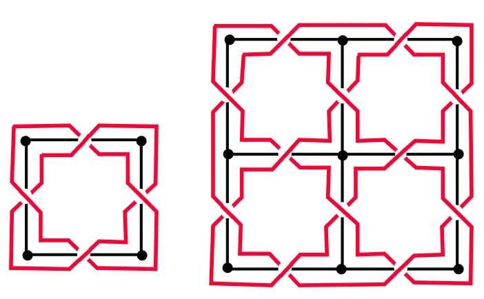
Figure 1: Graphs $(\mathbb{G}_{2})|_{R}$ and associated links, $\Lambda=\langle x_{1}^{2},x_{2}^{2}\rangle$ and $\langle x_{1}^{3},x_{2}^{3}\rangle$

The determinant of a link $\ell$, denoted here by $d(\ell)$, is the absolute value of its 1-variable Alexander polynomial evaluated at $-1$. We recall that a link $\ell$ is separable if some embedded $2$-sphere in ${\mathbb{S}}^{3}\setminus\ell$ bounds a $3$-ball containing a proper sublink of $\ell$. Otherwise $\ell$ is nonseparable. Any link is the union of nonseparable sublinks.

The determinant of a separable link vanishes. We denote by $D(\ell_{R})$ the nonzero product $d(\ell_{1})\cdots d(\ell_{r})$, where $\ell_{1},\ldots,\ell_{r}$ are the nonseparable sublinks that comprise $\ell$.

It follows from the Mayberry-Bott theorem [2] that if $\ell$ is an alternating link that arises by the medial construction from a finite plane graph, then $d(\ell)$ is equal to the number of spanning trees of the graph (see appendix A.4 in[3]). The following corollary is an immediate consequence of Theorem 3.6. It has been proven independently by Champanerkar and Kofman [5].

Corollary 3.9.

Let $G$ be a plane graph with cofinite free $\mathbb{Z}^{d}$-symmetry, $d\leq 2$. Then

$$\lim_{\langle\Lambda\rangle\to\infty}\frac{1}{|\mathbb{Z}^{d}/\Lambda|}\log D(\ell_{R})=m({\Delta}).$$

Remark 3.10.

(1) As in Theorem 3.6, if each $G|_{R}$ is connected, then no link $\ell_{R}$ is separable. In this case, $D(\ell_{R})$ is equal to the ordinary determinant of $\ell_{R}$.

(2) In [6] the authors consider as well as more general sequences of links. When $G=\mathbb{G}_{2}$, their results imply that:

$$\lim_{\langle\Lambda\rangle\to\infty}\frac{2\pi}{c(\ell_{R})}\log d(\ell_{R})=v_{oct},$$

where $c(\ell_{R})$ is the number of crossings of $\ell_{R}$ and $v_{oct}\approx 3.66386$ is the volume of the regular ideal octohedron.

Grid graphs are the simplest connected locally finite graphs admitting free $\mathbb{Z}^{d}$-symmetry, as the following theorem shows.

Theorem 3.11.

If $G$ is a graph with cofinite free $\mathbb{Z}^{d}$-symmetry and finitely many connected components, then $\gamma(G)\geq\gamma(\mathbb{G}_{d})$, and so $m({\Delta}(G))\geq m({\Delta}(\mathbb{G}_{d}))$.

Remark 3.12.

If $G$ has infinitely many connected components, then the conclusion of Theorem 3.11 need not hold. Consider, for example, the graph $\mathbb{G}_{2}$ with every vertical edge deleted. The graph has cofinite free $\mathbb{Z}^{2}$-symmetry. It follows from Lemma 4.2 below that its complexity growth rate is equal to $m({\Delta}(\mathbb{G}_{1}))=0$, which is less than $m({\Delta}(\mathbb{G}_{2}))$.

The following lemma, needed for the proof of Corollary 3.14, is of independent interest.

Lemma 3.13.

The sequence of complexity growth rates $m({\Delta}(\mathbb{G}_{d}))$ is nondecreasing.

Doubling each edge of $\mathbb{G}_{1}$ results in a graph with Laplacian polynomial $2(2-x-x^{-1})$, which has logarithmic Mahler measure $\log 2+m(2-x-x^{-1})=\log 2$. The following corollary states that this is minimum nonzero complexity growth rate.

Corollary 3.14.

(Complexity Growth Rate Gap) Let $G$ be any graph with cofinite free $\mathbb{Z}^{d}$-symmetry and Laplacian polynomial ${\Delta}$. If $m({\Delta})\neq 0$, then

$$m({\Delta})\geq\log 2.$$

Although ${\Delta}(\mathbb{G}_{d})$ is relatively simple, the task of computing its Mahler measure is not. It is well known and not difficult to see that $m({\Delta}(\mathbb{G}_{d}))\leq\log 2d$. We will use Alon’s result (Theorem 2.7) to show that $m(\mathbb{G}_{d})$ approaches $\log 2d$ asymptotically.

Theorem 3.15.

(1) For every $d\geq 1$, $m({\Delta}(\mathbb{G}_{d}))\leq\log 2d$.
(2) $\lim_{d\to\infty}m({\Delta}(\mathbb{G}_{d}))-\log 2d=0.$

Asymptotic results about the Mahler measure of certain families of polynomials have been obtained elsewhere. However, the graph theoretic methods that we employ to prove Theorem 3.11 are different from techniques used previously.

4 Algebraic dynamical systems and proofs.

We review some of the ideas of algebraic dynamical systems found in [17] and [20].

For any finitely generated module $M$ over ${\cal R}_{d}$, we can consider the Pontryagin dual $\widehat{M}={\rm Hom}(M,{\mathbb{T}})$, where ${\mathbb{T}}$ is the additive circle group $\mathbb{R}/\mathbb{Z}$. We regard $M$ as a discrete space. Endowed with the compact-open topology, $\widehat{M}$ is a compact $0$-dimensional space. Moreover, the module actions of $x_{1},\ldots,x_{d}$ determine commuting homeomorphisms $\sigma_{1},\ldots,\sigma_{d}$ of $\widehat{M}$. Explicitly, $(\sigma_{j}\rho)(a)=\rho(x_{j}a)$ for every $a\in M$. Consequently, $\widehat{M}$ has a $\mathbb{Z}^{d}$-action $\sigma:\mathbb{Z}^{d}\to\text{Aut}(\widehat{M})$. We will regard monomials $x^{\bf s}$ as acting on $\widehat{M}$ by $\sigma({\bf s})$ .

The pair $(\widehat{M},\sigma)$ is an algebraic dynamical system. It is well defined up to topological conjugacy; that is, up to a homeomorphism of $\widehat{M}$ respecting the $\mathbb{Z}^{d}$ action. In particular its periodic point structure is well defined.

Topological entropy $h(\sigma)$ is another well-defined quantity associated to $(\widehat{M},\sigma)$. (See [17] or [20] for the definition.) When $M$ can be presented by a square matrix $A$ with entries in ${\cal R}_{d}$, topological entropy can be computed as the logarithmic Mahler measure $m(\det A)$.

For any subgroup $\Lambda$ of $\mathbb{Z}^{d}$, a $\Lambda$-periodic point is an element that is fixed by every $x^{\bf s}\in\Lambda$. The set of all $\Lambda$-periodic points is denoted by ${\rm Per}_{\Lambda}(\sigma)$. It is a finitely generated abelian group isomorphic to ${\rm Hom}(T(M/\Lambda M),{\mathbb{T}})$, the Pontryagin dual of the torsion subgroup of $M/\Lambda M$. The group consists of $|T(M/\Lambda M)|$ tori of dimension equal to the rank of $M/\Lambda M$.

We apply the above ideas to graphs $G$ with cofinite free $\mathbb{Z}^{d}$-symmetry. As in [15], define the coloring module $C$ to be the finitely presented module over the ring ${\cal R}_{d}$ with presentation matrix equal to the $n\times n$ Laplacian matrix $L$ of $G$. The Laplacian polynomial ${\Delta}$ arises as the $0$th elementary divisor of $C$.

Let $\Lambda$ be a finite-index subgroup of $\mathbb{Z}^{d}$, and consider the $r$-sheeted covering graph $G_{\Lambda}$. It has finitely many connected components. We denote by $n_{\Lambda}$ the product of the cardinality of the vertex sets of the components. If $G$ is connected, then $n_{\Lambda}=|\overline{V}||\mathbb{Z}^{d}/\Lambda|$.

As in [20], let

$$\Omega(\Lambda)=\{{\bf c}=(c_{1},\ldots,c_{d})\in\mathbb{C}^{d}\mid{\bf c}^{\bf n}=1\ \forall\ {\bf n}=(n_{1},\ldots,n_{d})\in\Lambda\}.$$

The following combinatorial formula for the complexity $\tau(G_{\Lambda})$ is motivated by [14]. It is similar to the formula on page 621 of [17] and also page 191 of [20]. The proof here is relatively elementary.

Proposition 4.1.

Let $G$ be a graph with cofinite free $\mathbb{Z}^{d}$-symmetry. Let $\Lambda$ be a finite-index subgroup of $\mathbb{Z}^{d}$. If ${\Delta}$ is the Laplacian polynomial of $G$, then

$$T(G_{\Lambda})=\frac{1}{n_{\Lambda}}\prod_{{(c_{1},\ldots,c_{d})\in\Omega(\Lambda)\cap{\mathbb{S}}^{d}}\atop{{\Delta}(c_{1},\ldots,c_{d})\neq 0}}|{\Delta}(c_{1},\ldots,c_{d})|.$$ (4.1)

Proof.

Since $\Lambda$ has finite index in $\mathbb{Z}^{d}$, there exist positive integers $r_{1},\ldots,r_{d}$ such that $\mathbb{Z}^{d}/\Lambda\cong\mathbb{Z}/(r_{1})\oplus\cdots\oplus\mathbb{Z}/(r_{d})$. We can choose a basis $u_{1},\ldots,u_{d}$ for $\mathbb{Z}^{d}$ such that the coset of $u_{i}$ generates $\mathbb{Z}/(r_{i})$ (Theorem VI.4 of [19] can be used). Let ${\Delta}^{\prime}={\Delta}(u_{1},\cdots,u_{d})$. Equation 4.1 becomes:

$$T(G_{\Lambda})=\frac{1}{n_{\Lambda}}\prod_{{(\omega_{1}^{r_{1}},\ldots,\omega_{d}^{r_{d}})=(1,\ldots,1)}\atop{{\Delta}^{\prime}(\omega_{1},\ldots,\omega_{d})\neq 0}}|{\Delta}^{\prime}(\omega_{1},\ldots,\omega_{d})|.$$ (4.2)

Let $P_{r_{i}}$ denote the $r_{i}\times r_{i}$ permutation matrix corresponding to the cycle $(1,2,\ldots,r_{i})$. With respect to the basis $u_{1},\ldots,u_{d}$, the Laplacian matrix $L_{\Lambda}$ for $G_{\Lambda}$ can be obtained from the Laplacian matrix $L$ for $G$ by replacing each variable $u_{i}$ with the $r\times r$ tensor (Kronecker) product $U_{i}=I_{1}\otimes\cdots I_{i-1}\otimes P_{r_{i}}\otimes I_{i+1}\otimes\cdots I_{d}$. Here $I_{1},\cdots,I_{d}$ denote identity matrices of sizes $r_{1}\times r_{1},\ldots,r_{d}\times r_{d}$, respectively. Any scalar $c$ is replaced with $c$ times the $r\times r$ identity matrix. We regard $L_{\Lambda}$ as a block matrix with blocks of size $r\times r$.

By elementary properties of tensor product, the matrices $U_{i}$ commute. Hence the blocks of the characteristic matrix $\lambda I-L_{\Lambda}$ commute. The main result of [13] implies that the determinant of $\lambda I-L_{\Lambda}$ can be computed by treating the blocks as entries in a $d\times d$ matrix, computing the determinant, which is a single $r\times r$ matrix $D$, and finally computing the determinant of $D$.

The matrix $D$ is simply the Laplacian polynomial ${\Delta}^{\prime}(U_{1},\ldots,U_{d})$. The matrices $U_{i}$ can be simultaneously diagonalized. For each $i$, let $v_{i,1},\ldots,v_{i,r_{i}}$ be a basis of eigenvectors for $P_{i}$ with corresponding eigenvalues the $r_{i}$th roots of unity. Then $\{v_{1,j_{1}}\otimes\cdots\otimes v_{d,j_{d}}\mid 0\leq j_{i}<r_{i}\}\subset\mathbb{C}^{d}$ is a basis of eigenvectors for $D$. With respect to such a basis, $D$ is a diagonal matrix with diagonal entries ${\Delta}^{\prime}(\omega_{1},\ldots,\omega_{d})$, where $\omega_{i}$ is any $r_{i}$th root of unity. Using Corollary 2.6 and changing variables back, the proof is complete.

∎

Proof of Theorem 3.6. We must show that

$$\lim_{\langle\Lambda\rangle\to\infty}\frac{1}{|\mathbb{Z}^{d}/\Lambda|}\log T(G_{\Lambda})$$

exists and is equal to $m({\Delta})$ where ${\Delta}$ is the Laplacian polynomial of $G$. Consider the formula (4.1) for $T(G)$ given by Proposition 4.1. We will prove shortly that

$$\lim_{\langle\Lambda\rangle\to\infty}\frac{1}{|\mathbb{Z}^{d}/\Lambda|}\log n_{\Lambda}=0.$$

Assuming this, it suffices to show that

$$\lim_{\langle\Lambda\rangle\to\infty}\frac{1}{|\mathbb{Z}^{d}/\Lambda|}\log\prod|{\Delta}(c_{1},\ldots,c_{d})|=\lim_{\langle\Lambda\rangle\to\infty}\frac{1}{|\mathbb{Z}^{d}/\Lambda|}\sum\log|{\Delta}(c_{1},\ldots,c_{d})|=m({\Delta}).$$ (4.3)

Here the product and sum are over all $d$-tuples $(c_{1},\ldots,c_{d})\in\Omega(\Lambda)\cap{\mathbb{S}}^{d}$ such that ${\Delta}(c_{1},\ldots,c_{d})\neq 0$. By a unimodular change of basis, as in the proof of Proposition 4.1, we see that the second expression in (4.3) is a Riemann sum for $m({\Delta})$. The contribution of vanishingly small members of the partition that contain zeros of ${\Delta}$ can be made arbitrarily small (see pages 58–59 of [7]). Hence the Riemann sums converge to $m({\Delta})$.

It remains to show that $\lim_{\langle\Lambda\rangle\to\infty}\frac{1}{|\mathbb{Z}^{d}/\Lambda|}n_{\Lambda}=0.$ For this it suffices to assume that $G$ is the $\mathbb{Z}^{d}$ orbit of a single, unbounded component. Then $G_{\Lambda}$ is also the orbit of a single component $G_{0}$. It is stabilized by some nonzero element $w\in{\cal R}_{d}$. The cardinality $|V(G_{0})|$ is at least as large as the cardinality of the orbit of the identity in $\mathbb{Z}^{d}/\Lambda$ under translation by $w$. The line through the origin in the direction of $w$ intersects the fundamental region of $\mathbb{Z}^{d}/\Lambda$ in a segment of length at least as $\langle\Lambda\rangle$. Hence the cardinality of the orbit of the origin under $w$ is at least $\langle\Lambda\rangle/|w|$. From this we conclude that

$$|V(G_{0})|\geq\frac{\langle\Lambda\rangle}{|w|}.$$

To complete the argument, let $N=|\overline{V}||\mathbb{Z}^{d}/\Lambda|$ denote the number of vertices in $G_{\Lambda}$. Let $k$ be the number of connected components of $G_{\Lambda}$. Since the components are graph isomorphic (by the induced $\mathbb{Z}^{d}$ action), $n_{\Lambda}$ is equal to $(N/k)^{k}$. Now

$$\lim_{\langle\Lambda\rangle\to\infty}\frac{1}{|\mathbb{Z}^{d}/\Lambda|}\log n_{\Lambda}=\lim_{\langle\Lambda\rangle\to\infty}\frac{1}{|\mathbb{Z}^{d}/\Lambda|}\log\bigg{(}\frac{N}{k}\bigg{)}^{k}.$$

Letting $s=N/k$, the number of vertices in each component, we have

$$\lim_{\langle\Lambda\rangle\to\infty}\frac{1}{|\mathbb{Z}^{d}/\Lambda|}\log(s)^{\frac{N}{s}}=|\overline{V}|\lim_{\langle\Lambda\rangle\to\infty}\frac{\log s}{s}.$$

The last limit is zero since $s$ must grow without bound. ∎

Now suppose $H$ is a subgraph of $G$ consisting of one or more connected components of $G$, such that the orbit of $H$ under $\mathbb{Z}^{d}$ is all of $G$. Let $\Gamma<\mathbb{Z}^{d}$ be the stabilizer of $H$. Then $\Gamma\cong\mathbb{Z}^{d^{\prime}}$ for some $d^{\prime}\leq d$, and its action on $H$ can be regarded as a cofinite free action of $\mathbb{Z}^{d^{\prime}}$. Its complexity growth rate is given by

$${\gamma}(H)=\lim_{{\langle}\Lambda{\rangle}\to\infty}\frac{1}{|\Gamma/\Lambda|}\log T(H_{\Lambda})$$

where $\Lambda$ ranges over finite-index subgroups of $\Gamma$.

Lemma 4.2.

Under the above conditions we have ${\gamma}(G)={\gamma}(H)$.

Proof.

Let $\Lambda$ be any finite-index subgroup of $\mathbb{Z}^{d}$. Then $H$ is invariant under $\Lambda\cap{\Gamma}$. The image of $H$ in the quotient graph $G_{\Lambda}$ is isomorphic to $H_{\Lambda\cap{\Gamma}}$.

Note that the quotient $\overline{H}$ of $H$ by the action of ${\Gamma}$ is isomorphic to $\overline{G}$, since the $\mathbb{Z}^{d}$ orbit of $H$ is all of $G$. Since $G_{\Lambda}$ is a $|\mathbb{Z}^{d}/\Lambda|$-fold cover of $\overline{G}$ and $H_{\Lambda\cap{\Gamma}}$ is a $|{\Gamma}/(\Lambda\cap{\Gamma})|$-fold cover of $\overline{H}$, $G_{\Lambda}$ comprises $k=|\mathbb{Z}^{d}/\Lambda|/|{\Gamma}/(\Lambda\cap{\Gamma})|$ mutually disjoint translates of a graph that is isomorphic to $H_{\Lambda\cap{\Gamma}}$. Hence $T(G_{\Lambda})=T(H_{\Lambda\cap{\Gamma}})^{k}$ and

$$\frac{1}{|\mathbb{Z}^{d}/\Lambda|}\log T(G_{\Lambda})=\frac{1}{|{\Gamma}/(\Lambda\cap{\Gamma})|}\log T(H_{\Lambda\cap{\Gamma}}).$$

Since ${\langle}\Lambda\cap{\Gamma}{\rangle}\to\infty$ as ${\langle}\Lambda{\rangle}\to\infty$, we have ${\gamma}(G)={\gamma}(H)$. ∎

Proof of Theorem 3.11. By Proposition 3.2, we may assume that $G$ is the orbit of a single connected component $H$. Since $G$ has finitely many components, the stabilizer ${\Gamma}$ of $H$ is isomorphic to $\mathbb{Z}^{d}$ and has a cofinite free action on $H$, with ${\gamma}(G)={\gamma}(H)$ by Lemma 4.2. Thus we can assume $G$ is connected.

Consider the case in which $G$ has a single vertex orbit. Then for some $u_{1},\ldots,u_{m}\in\mathbb{Z}^{d}$, the edge set $E$ consists of edges from $v$ to $u_{i}\cdot v$ for each $v\in V$ and $i=1,\ldots,m$. Since $G$ is connected, we can assume after relabeling that $u_{1},\ldots,u_{d}$ generate a finite-index subgroup of $\mathbb{Z}^{d}$. Let $G^{\prime}$ be the be the $\mathbb{Z}^{d}$-invariant subgraph of $G$ with edges from $v$ to $u_{i}\cdot v$ for each $v\in V$ and $i=1,\ldots,d$. Then $G^{\prime}$ is the orbit of a subgraph of $G$ that is isomorphic to $\mathbb{G}_{d}$, and so by Lemma 4.2, ${\gamma}(\mathbb{G}_{d})={\gamma}(G^{\prime})\leq{\gamma}(G)$.

We now consider a connected graph $G$ having vertex families $v_{1,{\bf s}},\ldots,v_{n,{\bf s}}$, where $n>1$. Since $G$ is connected, there exists an edge $e$ joining $v_{1,{\bf 0}}$ to some $v_{2,{\bf s}}$. Contract the edge orbit $\mathbb{Z}^{d}\cdot e$ to obtain a new graph $G^{\prime}$ having cofinite free $\mathbb{Z}^{d}$-symmetry and complexity growth rate no greater than that of $G$. Repeat the procedure with the remaining vertex families so that only $v_{1,{\bf s}}$ remains. The proof in the previous case of a graph with a single vertex orbit now applies. ∎

Proof of Lemma 3.13. Consider the grid graph $\mathbb{G}_{d}$. Deleting all edges in parallel to the $d$th coordinate axis yields a subgraph $G$ consisting of countably many mutually disjoint translates of $\mathbb{G}_{d-1}$. By Lemma 4.2, $m({\Delta}(\mathbb{G}_{d-1}))=m({\Delta}(G))\leq m({\Delta}(\mathbb{G}_{d}))$. ∎

Proof of Corollary 3.14. By Proposition 3.2 and Lemma 4.2, it suffices to consider a connected graph $G$ with cofinite free $\mathbb{Z}^{d}$-symmetry and $m({\Delta}(G))$ nonzero. Note that $m(\mathbb{G}_{1})=0$ while $m(\mathbb{G}_{2})\approx 1.166$ is greater than $\log 2$. By Theorem 3.11 and Lemma 3.13 we can assume that $d=1$.

If $G$ has an orbit of parallel edges, we see easily that ${\gamma}(G)\geq\log 2$. Otherwise, we proceed as in the proof of Theorem 3.11, contracting edge orbits to reduce the number of vertex orbits without increasing the complexity growth rate. If at any step we obtain an orbit of parallel edges, we are done; otherwise we will obtain a graph $G^{\prime}$ with a single vertex orbit and no loops. If $G^{\prime}$ is isomorphic to $\mathbb{G}_{1}$ then $G$ must be a tree; but then $m({\Delta}(G))={\gamma}(G)=0$, contrary to our hypothesis. So $G^{\prime}$ must have at least two edge orbits. Deleting excess edges, we may suppose $G^{\prime}$ has exactly two edge orbits.

The Laplacian polynomial $m({\Delta}(G^{\prime}))$ has the form $4-x^{r}-x^{-r}-x^{s}-x^{-s}$, for some positive integers $r,s$. Reordering the vertex set of $G^{\prime}$, we can assume without loss of generality that $r=1$. The following calculation is based on an idea suggested to us by Matilde Lalin.

$$m({\Delta}(G^{\prime}))=\int_{0}^{1}\log|4-2\cos(2\pi\theta)-2\cos(2\pi s\theta)|\ d\theta$$

$$=\int_{0}^{1}\log|2(1-\cos(2\pi\theta))+2(1-\cos(2\pi s\theta))|\ d\theta$$

$$=\int_{0}^{1}\log\bigg{(}4\sin^{2}(\pi\theta)+4\sin^{2}(\pi s\theta)\bigg{)}\ d\theta.$$

Using the inequality $(u^{2}+v^{2})\geq 2uv$, for any nonnegative $u,v$, we have:

$$m({\Delta}(G^{\prime}))\geq\int_{0}^{1}\log\bigg{(}8|\sin(\pi\theta)|\ |\sin(\pi s\theta)|\bigg{)}\ d\theta$$

$$=\log 8+\int_{0}^{1}\log|\sin(\pi\theta)|\ d\theta+\int_{0}^{1}\log|\sin(\pi s\theta)|\ d\theta$$

$$=\log 8+\int_{0}^{1}\log\sqrt{\frac{1-\cos(2\pi\theta)}{2}}\ d\theta+\int_{0}^{1}\log\sqrt{\frac{1-\cos(2\pi s\theta)}{2}}\ d\theta$$

$$=\log 8+\int_{0}^{1}\frac{1}{2}\log\bigg{(}\frac{2-2\cos(2\pi\theta)}{4}\bigg{)}\ d\theta+\int_{0}^{1}\frac{1}{2}\log\bigg{(}\frac{2-2\cos(2\pi s\theta)}{4}\bigg{)}\ d\theta$$

$$=\log 8+\frac{1}{2}m(2-x-x^{-1})-\frac{1}{2}\log 4+\frac{1}{2}m(2-x^{s}-x^{-s})-\frac{1}{2}\log 4$$

$$=3\log 2+0-\log 2+0-\log 2=\log 2.$$

∎

Proof of Theorem 3.15. (1) The integral representing the logarithmic Mahler measure of ${\Delta}(\mathbb{G}_{d})$ can be written

$$\int_{0}^{1}\cdots\int_{0}^{1}\log\bigg{|}2d-\sum_{i=1}^{d}2\cos(2\pi\theta_{i})\bigg{|}d\theta_{1}\cdots d\theta_{d}$$

$$=\log 2d+\int_{0}^{1}\cdots\int_{0}^{1}\log\bigg{|}1+\sum_{i=1}^{d}\frac{\cos(2\pi\theta_{i})}{d}\bigg{|}d\theta_{1}\cdots d\theta_{d}$$

$$=\log 2d+\int_{0}^{1}\cdots\int_{0}^{1}-\sum_{k=1}^{\infty}\frac{(-1)^{k}}{k}\bigg{(}\frac{\sum_{i=1}^{d}\cos(2\pi\theta_{i})}{d}\bigg{)}^{k}d\theta_{1}\cdots d\theta_{d}.$$

By symmetry, odd powers of $k$ in the summation contribute zero to the integration. Hence

$$m({\Delta}(\mathbb{G}_{d})=\log 2d-\int_{0}^{1}\cdots\int_{0}^{1}\sum_{k=1}^{\infty}\frac{1}{2k}\bigg{(}\frac{\sum_{i=1}^{d}\cos(2\pi\theta_{i})}{d}\bigg{)}^{2k}d\theta_{1}\cdots d\theta_{d}\leq\log 2d.$$

(2) Let $\Lambda$ be a finite-index subgroup of $\mathbb{Z}^{d}$. Consider the quotient graph $(\mathbb{G}_{d})_{\Lambda}$. The cardinality of its vertex set is $|\mathbb{Z}^{d}/\Lambda|$. The main result of [1], cited above as Theorem 2.7, implies that

$$\tau((\mathbb{G}_{d})_{\Lambda})=\bigg{(}(2d)(1-\mu(d))\bigg{)}^{|\mathbb{Z}^{d}/\Lambda|},$$

where $\mu$ is a nonnegative function such that $\lim_{d\to\infty}\mu(d)=0$. Hence

$$\lim_{d\to\infty}\bigg{(}\frac{1}{|\mathbb{Z}^{d}/\Lambda|}\log\tau((\mathbb{G}_{d})_{\Lambda}-\log 2d\bigg{)}=\lim_{d\to\infty}\log(1-\mu(d))=0.$$

Theorem 3.6 completes the proof. ∎

Remark 4.3.

One can evaluate $m({\Delta}(\mathbb{G}_{d}))$ numerically and obtain an infinite series representing $m({\Delta}(\mathbb{G}_{d}))-\log 2d$. However, showing rigorously that the sum of the series approaches zero as $d$ goes to infinity appears to be difficult. (See [21], p. 16 for a heuristic argument.)

Department of Mathematics and Statistics,
University of South Alabama
Mobile, AL 36688 USA
Email:
silver@southalabama.edu
swilliam@southalabama.edu

References

- [1] N. Alon, The number of spanning trees in regular graphs, in: Random Structures and Algorithms, Vol. 1, No. 2 (1990), 175–181.
- [2] A. Bott and J.P. Mayberry, Matrices and trees, in Economic Activity Analysis (O. Morgenstern, ed.), 391–400, Wiley, New York, 1954.
- [3] G. Burde, H. Zieschang, Knots, Walter de Gruyter and Co., Berlin, 1985.
- [4] R. Burton and R. Pemantle, Local characteristics, entropy and limit theorems for spanning trees and domino tilings via transfer-impedances, Ann. Prob. 21 (1993), 1329–1371.
- [5] A. Champanerkar I. Kofman, The determinant density and biperiodic alternating links, in preparation.
- [6] A. Champanerkar, I. Kofman and J.S. Purcell, Geometrically and diagrammatically maximal knots, preprint, 2015 arXiv:1411.7915v3
- [7] G. Everest and T. Ward, Heights of Polynomials and Entropy in Algebraic Dynamics, Springer-Verlag, London 1999.
- [8] R. Forman, Determinants of Laplacians on graphs, Topology, 32 (1993), 35–46. 109–113.
- [9] C. Godsil, G. Royle, Algebraic Graph Theory, Springer Verlag, 2001.
- [10] G.R. Grimmett, An upper bound for the number of spanning trees of a graph, Discrete Math. 16 (1976), 323–324.
- [11] L.H. Kauffman, Knots and Physics, Third Edition, World Scientific, Singapore, 2001.
- [12] R. Kenyon, The Laplacian on planar graphs and graphs on surfaces, in Current Developments in Mathematics (2011), 1 – 68.
- [13] I. Kovacs, D.S. Silver and S.G. Williams, Determinants of commuting-block matrices, American Mathematical Monthly 106 (1999), 950–952.
- [14] G. Kreweras, Complexité et circuits Eulériens dans les sommes tensorielles de graphes, J. Comb. Theory, Series B 24 (1978), 202–212.
- [15] K.R. Lamey, D.S. Silver and S.G. Williams, Vertex-colored graphs, bicycle spaces and Mahler measure, preprint (2014), arXiv:1408.6570
- [16] D.A. Lind, Dynamical properties of quasihyperbolic toral automorphisms, Ergod. Th. and Dynam. Sys. 2 (1982), 49–68.
- [17] D.A. Lind, K. Schmidt and T. Ward, Mahler measure and entropy for commuting automorphisms of compact groups, Inventiones Math. 101 (1990), 593–629.
- [18] R. Lyons, Asymptotic enumeration of spanning trees, Probability and Computing 14 (2005), 491–522.
- [19] J. Rotman, An Introduction to the Theory of Groups, 4th edition, Springer-Verlag, Berlin, 1995.
- [20] K. Schmidt, Dynamical Systems of Algebraic Origin, Birkhäuser, Basel, 1995.
- [21] R. Shrock and F.Y. Wu, Spanning trees on graphs and lattices in dimensions, J. Phys. A: Math. Gen. 33 (2000), 3881–3902.
- [22] R. Solomyak, On coincidence of entropies for two classes of dynamical systems, Ergod. Th. & Dynam. Sys. 18 (1998), 731–738.
- [23] F.Y. Wu, Number of spanning trees on a lattice. J. Phys. A, 10(6) L113, 1977.