Comments on “On Clock Synchronization Algorithms for Wireless Sensor Networks Under Unknown Delay”

Abstract

The generalization of the maximum-likelihood-like estimator for clock skew by Leng and Wu in the above paper is erroneous because the correlation of the noise components in the model is not taken into account in the derivation of the maximum likelihood estimator, its performance bound, and the optimal selection of the gap between two subtracting time stamps. This comment investigates the issue of noise correlation in the model and provides the range of the gap for which the maximum likelihood estimator and its performance bound are valid and corrects the optimal selection of the gap based on the provided range.

 

As one of the three clock-synchronization algorithms studied for wireless sensor networks (WSNs) under unknown delay [1], Leng and Wu proposed the generalization of the maximum-likelihood-like estimator (MLLE) proposed by Noh et al. [2]. To overcome the drawback of the MLLE that it can utilize only the time stamps in the first and the last of $N$ message exchanges, they extend the gap $\alpha$ between two subtracting time stamps from $N{-}1$ to a range of $\left[1,\ldots,N{-}1\right]$ so that the generalized MLLE can take into more time stamps in estimating clock skew.

Specifically, the time stamps in two-way message exchanges are modeled as [1, Eqs. (1) and (2)]

$$T_{2,i} =\beta_{1}T_{1,i}+\beta_{0}+\beta_{1}\left(d+X_{i}\right)$$ (1)

$$T_{3,i} =\beta_{1}T_{4,i}+\beta_{0}-\beta_{1}\left(d+Y_{i}\right)$$ (2)

where $\beta_{0}$ and $\beta_{1}$ denote the clock offset and clock skew of the child node $S$ with respect to the parent node $P$, respectively; $d$ represents the fixed portion of one-way propagation delay, while $X_{i}$ and $Y_{i}$ are its variable portions (see Fig. 1 of [1]). Based on (1) and (2), they construct new sequences $D_{r,j}{\triangleq}T_{r,\alpha+j}{-}T_{r,j}$ ($j{=}1,\ldots,N{-}\alpha$ and $r{=}1,2,3,4$) and model them as follows [1, Eqs. (10) and (11)]:

$$D_{2,j} =\beta_{1}D_{1,j}+\beta_{1}\left(X_{\alpha+j}-X_{j}\right)$$ (3)

$$D_{3,j} =\beta_{1}D_{4,j}-\beta_{1}\left(Y_{\alpha+j}-Y_{j}\right)$$ (4)

for $j{=}1,\ldots,N{-}\alpha$. Noting that $\left(X_{\alpha+j}{-}X_{j}\right){\sim}\mathcal{N}(0,2\sigma^{2})$ and $\left(Y_{\alpha+j}{-}Y_{j}\right){\sim}\mathcal{N}(0,2\sigma^{2})$ because $X_{j}$ and $Y_{j}$ are i.i.d. zero-mean Gaussian random variables with variance $\sigma^{2}$, they obtain the maximum-likelihood estimator (MLE) for $\beta_{1}$ given by [1, Eq. (13)]

$$\hat{\beta}_{1}=\dfrac{1}{\hat{\theta}_{1}}=\dfrac{\sum_{j=1}^{N-\alpha}\left(D_{2,j}^{2}+D_{3,j}^{2}\right)}{\sum_{j=1}^{N-\alpha}\left(D_{1,j}D_{2,j}+D_{4,j}D_{3,j}\right)}.$$ (5)

The major problem in the derivation of the MLE for $\beta_{1}$ given in (5) is that, even though $X_{j}$ and $Y_{j}$ are i.i.d. Gaussian random variables, the noise components $\left(X_{\alpha+j}{-}X_{j}\right)$ and $\left(Y_{\alpha+j}{-}Y_{j}\right)$ are not in general: For $m,n{\in}\left\{1,\ldots,N-\alpha\right\}$ and $m{\neq}n$,

$$\operatorname{E}\left[\left(X_{\alpha+m}-X_{m}\right)\left(X_{\alpha+n}-X_{n}\right)\right]$$

$$=-\operatorname{E}\left[X_{\alpha+m}X_{n}\right]-\operatorname{E}\left[X_{m}X_{\alpha+n}\right]$$

$$=\begin{cases}-\sigma^{2},&\mbox{if }\alpha=\left|m-n\right|\\ 0,&\mbox{otherwise}\end{cases},$$ (6)

and the same goes for $\left(Y_{\alpha+j}{-}Y_{j}\right)$. Note that, if the noise components are independent one another as claimed in [1], the expectation in ( ‣ Comments on “On Clock Synchronization Algorithms for Wireless Sensor Networks Under Unknown Delay”) must be zero.

The consequence of ( ‣ Comments on “On Clock Synchronization Algorithms for Wireless Sensor Networks Under Unknown Delay”) is that $\alpha$ should be greater than $\frac{N-1}{2}$, i.e.,

$$\alpha\in\left\{\left\lfloor\frac{N}{2}\right\rfloor,\ldots,N-1\right\}$$ (7)

in order to maintain the validity of the derivation of the MLE for $\beta_{1}$ [1, Eq. (13)] and its performance bound [1, Eq. (29)]: If $\alpha{\leq}\frac{N-1}{2}$, there exists at least one pair of $m$ and $n$ satisfying $\alpha=\left|m-n\right|$ so that the noise components are no longer independent one another. For example, let $n$ be 1. Then $m{=}\alpha{+}1$ satisfies the said condition. Because $\alpha{\leq}\frac{N-1}{2}$ and

$$m=\alpha+1\leq\dfrac{N-1}{2}+1=\dfrac{N+1}{2}=N-\dfrac{N-1}{2}\leq N-\alpha,$$

$m$ belongs to $\left\{1,\ldots,N-\alpha\right\}$.

Fig. 1 clearly shows the effect of the noise correlation on the mean square error (MSE) of estimation of clock skew and the relationship between $\alpha$ and $N$ when SNR=30 dB and $H{=}G{=}10$. In the figure, GE1 denotes the simulation results of the generalized MLLE for time stamps and resulting sequences generated according to the original models of (1) through (4); GE2, on the other hand, denotes the results for the time sequences in (3) and (4) with the noise components $\left(X_{\alpha+j}-X_{j}\right)$ and $\left(Y_{\alpha+j}-Y_{j}\right)$ replaced by two newly-generated i.i.d. zero-mean Gaussian random variables with variance $2\sigma^{2}$.

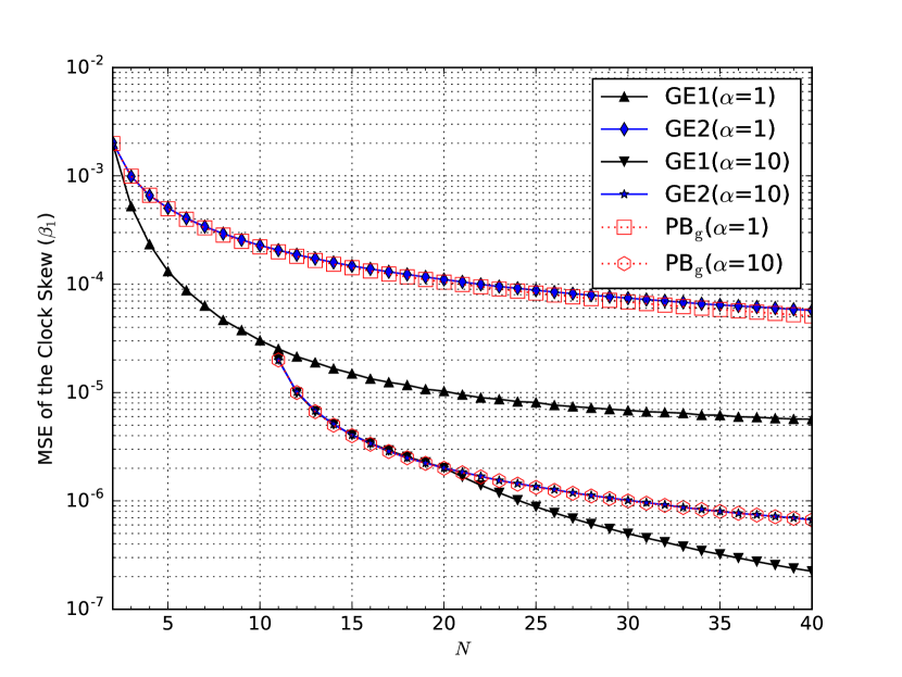
Figure 1: Effect of noise correlation on the MSE of estimated clock skew.

If $\alpha$ is greater than $\frac{N-1}{2}$, we can see that the results of GE1 closely match with the performance bounds (i.e., PB_g) because there is no issue of noise correlation; for example, when $\alpha$ is 10, the results of GE1 match with the performance bounds for $N$ up to 20. Compared to the results for GE1, the results for GE2 of a fictitious model show that they can attain the performance bounds irrespective of the value of $\alpha$ because there is no issue of noise correlation at all. It is interesting, though, that the results of GE1 for $\alpha\leq\frac{N-1}{2}$ show even better performance than the performance bounds.

With the valid range of $\alpha$ given by (7), the selection of the optimal $\alpha$ given in Eqs. (32) and (33) of [1] should be modified accordingly. Because $\Phi(\alpha_{r})$ in Eq. (32) of [1] is concave downward for the whole range of real-valued $\alpha_{r}{\in}\left[\left\lfloor\frac{N}{2}\right\rfloor,N{-}1\right]$, $\alpha^{*}_{r}$ in Eq. (33) of [1] is now simplified as follows:

$$\alpha^{*}_{r}=\dfrac{1}{3}N+\sqrt{\dfrac{1}{9}N^{2}-\dfrac{2\beta_{1}^{2}\sigma^{2}}{\beta_{1}^{2}H^{2}+G^{2}}}$$ (8)

References

- [1] M. Leng and Y.-C. Wu, “On clock synchronization algorithms for wireless sensor networks under unknown delay,” IEEE Trans. Veh. Technol., vol. 59, no. 1, pp. 182–190, Jan. 2010.
- [2] K.-L. Noh, Q. M. Chaudhari, E. Serpedin, and B. W. Suter, “Novel clock phase offset and skew estimation using two-way timing message exchanges for wireless sensor networks,” IEEE Trans. Commun., vol. 55, no. 4, pp. 766–777, Apr. 2007.