Wigner crystal phases in bilayer graphene

Abstract

It is generally believed that a Wigner Crystal in single layer graphene can not form because the magnitudes of the Coulomb interaction and the kinetic energy scale similarly with decreasing electron density. However, this scaling argument does not hold for the low energy states in bilayer graphene. We consider the formation of a Wigner Crystal in weakly doped bilayer graphene with an energy gap opened by a perpendicular electric field. We argue that in this system the formation of the Wigner Crystal is not only possible, but different phases of the crystal with very peculiar properties may exist here depending on the system parameters.

1. Introduction. – The observation of a Wigner crystal Wigner34 ; Bonsall79 ; Tanatar89 ; Drumond09 , a solidified phase of a conducting electron Fermi liquid, is a challenging task even in conventional metals Helium79 ; EAndrey88 ; Yoon99 . Finding, whether this elusive electron solid may exist in novel materials, like graphene, constitutes an additional challenge. Simple scaling analysis shows that Wigner crystallization in single layer graphene is unlikely Balatsky06 . Much richer is the issue of crystallization in bilayer graphene. If the gap in the bilayer electron spectrum is not opened, screening of the Coulomb interaction Hwang08 prevents the formation of the crystal, as we discuss below endnote . However, and this is the main result of this paper, if the gap is opened due to an interlayer voltage, the crystallization is not only possible, but depending on the density of electrons in the conduction band there should exist two very distinct phases of the crystal.

Interaction induced phases of undoped bilayer graphene have been addressed by numerous publications Nilsson06 ; Min08 ; McDonald10 ; Vafek10 ; NandkishorePRL10 ; NandkishorePRB10 ; Lemonik10 ; Throckmorton12 ; Throckmorton14 . The considered effects include the spontaneous ferromagnetic and/or pseudospin polarization Nilsson06 ; Min08 or the spontaneous gap opening in the electron’s spectrum NandkishorePRL10 ; NandkishorePRB10 , but not the spontaneous translation symmetry breaking. The spatial in-plane charge inhomogeneity is hard to expect in undoped bilayer graphene. In this paper we consider the breaking of translation symmetry in the form of an electron crystal in the case of a weakly doped conduction band in gapped bilayer graphene. A gate tunable doping level is obtained routinely in both single- and bilayer graphene Novosel05 ; Zhang05 .

Generally, Wigner crystallization takes place when the lowering of electrons’ repulsion energy in the crystal phase wins over the rise of the kinetic energy caused by the restricted motion on the lattice Wigner34 . Both the kinetic energy and the screened interaction behave highly nontrivially in bilayer graphene with the interlayer voltage induced gap. After the gap is opened, graphene becomes an insulator and electrons’ repulsion at very large distances becomes the usual Coulomb-law. However, at least one of the Wigner crystal phases, which we consider, exists for the inter-electron distances where the electrons’ interaction is well approximated by a logarithmic repulsion, reminiscent of the vortex interaction in type II superconductors Abrikosov57 ; SBook .

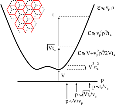
Figure 1: Schematic drawing of the different regimes for the kinetic energy dispersion $\varepsilon(p)$ in bilayer graphene with a gap opened by an interlayer voltage $V$ and with interlayer hopping energy $t_{\perp}$. Momentum is calculated from either $K$ or $K^{\prime}$ point. The inset shows the bilayer graphene lattice with Bernal AB-stacking.

Deep in the stable crystal phase, which is the only regime accessible analytically, the dominant repulsion of electrons favors the triangular lattice Bonsall79 with only small fluctuations around it. The kinetic energy, which has a unique form for electrons in bilayer graphene, is responsible in this regime for quantum fluctuations and small distortions of the classical lattice. These fluctuations may or may not respect the symmetries of the original triangular lattice. For example, the lattice symmetry is preserved at the quantum level in a Wigner crystal with quadratic dispersion ($\varepsilon\sim p^{2}/2m$) but is broken in 2-dimensional semiconductors with strong spin-orbit interaction Berg12 ; Silvestrov14 . As we will show, both of these possibilities are realized in gapped bilayer graphene at different electron densities.

Applying an interlayer voltage, besides opening the gap, leads to a peculiar single-electron dispersion with several regions of different scaling behavior as a function of momentum (see Fig. 1). Consequently, the two phases of the crystal, which we predict in this work, are distinguished by different kinetic energy dispersions at different electron densities. While the doping level in the conduction band is lowered, the dilute electron gas crystalizes into what we call an intermediate density crystal phase with a quartic electron dispersion, $\varepsilon(p)\propto p^{4}$. This anharmonic kinetic energy makes it difficult to describe the quantum fluctuations of the crystal. We use the self-consistent mean-field approximation to calculate the effective phonon modes in this case, which may be reasonable even in the absence of a small parameter. The quantum corrections in the case of $\varepsilon(p)\propto p^{4}$ obviously preserve the symmetries of the triangular crystal lattice.

When reducing the density of electrons further their energies get close to the bottom of the sombrero-like spectrum characteristic of graphene with an interlayer voltage McCann06 . This dispersion relation is reminiscent of the one for electrons with Rashba spin-orbit interaction Rashba60 . The Wigner crystallization in a two-dimensional electron gas with strong spin-orbit interaction was investigated in Refs. Berg12 ; Silvestrov14 . The predictions of Ref. Silvestrov14 , where the long-range interaction between electrons was assumed, may be applied to bilayer graphene almost without modifications. The main effect for the fluctuations in this low-density regime for bilayer graphene is an asymmetric (cigar-shape) density profile in real as well as momentum space which breaks the symmetries of the original triangular lattice. The fact that the two low energy phases of the electron crystal which we find have different symmetries rules out the possibility of a smooth crossover between them (see also Fig. (2)).

Taking into account properly the screening of electron-electron interaction is crucial for the correct description of Wigner crystallization in bilayer graphene. We describe below different screening regimes for the case of a parametrically small gap in bilayer graphene and give more details on the screening in the Appendix.

2. Bilayer graphene.– The Bloch Hamiltonian for the Bernal stacked bilayer graphene in the vicinity of the $K$ point is given by the matrix McCann06 (we neglect the hopping elements leading to the small trigonal warping terms)

$${\cal H}_{\mathbf{p}}=\left(\begin{array}[]{cc}-V\ \ \ \ \ \ v_{F}{\tilde{p}}\ \ \ \ 0\ \ \ \ \ 0\\ v_{F}{\tilde{p}}^{*}\ \ -V\ \ \ \ t_{\perp}\ \ \ \ \ 0\\ \ \ \ \ 0\ \ \ \ \ \ \ \ t_{\perp}\ \ \ \ \ V\ \ \ \ v_{F}{\tilde{p}}\\ \ \ 0\ \ \ \ \ \ \ \ 0\ \ \ \ v_{F}{\tilde{p}}^{*}\ \ \ V\end{array}\right)\ .$$ (5)

Here $\mathbf{p}$ is the momentum calculated from the $K$ point and ${\tilde{p}}=p_{x}+ip_{y}$. The hopping matrix element between two vertically aligned carbon atoms $t_{\perp}\approx 0.39\,{\rm eV}$ is small compared to the interlayer matrix element $t\approx 2.8\,{\rm eV}$, the latter entering Eq. (5) through the Fermi velocity $\hbar v_{F}=3dt/2$ with $d\approx 1.42$Å being the distance between two nearest in-plane carbon atoms. The layer potential $\pm V$ is regulated by the external gates. Each single electron state is doubly degenerate due to spin and electrons with momenta close to the $K^{\prime}$ point are described by the Hamiltonian ${\cal H}^{*}_{-\mathbf{p}}$.

Diagonalization of ${\cal H}_{\mathbf{p}}$ gives the particle-hole symmetric spectrum

$$\varepsilon^{2}=V^{2}+v_{F}^{2}p^{2}+\frac{t_{\perp}^{2}}{2}\pm\sqrt{v_{F}^{2}p^{2}(4V^{2}+t_{\perp}^{2})+\frac{t_{\perp}^{4}}{4}}.$$ (6)

For an interlayer voltage small compared to the interlayer hopping matrix element $V/t_{\perp}\ll 1$, the two crystal phases exist at parametrically different electron densities. The ratio $V/t_{\perp}$, which is a small parameter in our estimates, may be tuned experimentally. Assuming $V\ll t_{\perp}\ll t$, we find several distinct regimes of the spectrum Eq. (6),

$${\rm I.} \ \ \varepsilon\approx v_{F}p\ \ \ {\rm for}\ \ \ v_{F}p\gg t_{\perp}\ ,$$ (7)

$${\rm II.} \ \ \varepsilon\approx{v_{F}^{2}p^{2}}/{t_{\perp}}\ \ \ {\rm for}\ \ \ \sqrt{Vt_{\perp}}\ll v_{F}p\ll t_{\perp}\ ,$$

$${\rm III.} \ \ \varepsilon\approx V+\frac{v_{F}^{4}p^{4}}{2Vt_{\perp}^{2}}\ \ \ {\rm for}\ \ \ V\ll v_{F}p\ll\sqrt{Vt_{\perp}}\ ,$$

$${\rm IV.} \ \ \varepsilon\approx V-2V\frac{v_{F}^{2}p^{2}}{t_{\perp}^{2}}+\frac{v_{F}^{4}p^{4}}{2Vt_{\perp}^{2}}\ \ \ {\rm for}\ \ \ v_{F}p\sim V\ .$$

We show here only the low energy positive branch of solutions Eq. (6). Replacing the momentum by the inverse typical distance between electrons, $p\sim\sqrt{n}$, one finds the electron density $n$ assigned to each energy regime I-IV.

As we discuss below, Wigner crystallization is possible only in the lowest energy/density regimes III and IV of Eq. (7).

3. Screening of the Coulomb interaction.– The different energy dispersion regimes in Eq. (7) lead to a different ability of bilayer graphene to screen the coulombic electron-electron interaction at different length scales. We give a detailed description of the screening in the Appendix, and present here only the results.

First, at the highest energies or electron densities, the two graphene sheets are approximately decoupled, leading to a single-layer-like Coulomb interaction KotovRMP12 ,

$$U(r)={e^{2}}/{\epsilon\,r},$$ (8)

where the polarization of both the substrate and the graphene flake contribute similarly to the dielectric constant $\epsilon\sim 1$ (see Appendix).

The long-range Coulomb interaction in undoped intrinsic bilayer graphene is fully screened in the second regime II of Eq. (7) with quadratic dispersion and negligible gap, $\varepsilon\propto p^{2}$. The random-phase-approximation calculation of Ref. Hwang08 here gives

$$U(r\gg 1/q_{\rm TF})\sim{e^{2}}/{(q_{\rm TF}r)^{2}r}\ ,$$ (9)

where the Thomas-Fermy screening wave-vector $q_{\rm TF}\sim t_{\perp}/\hbar v_{\rm F}$ (see Appendix for details). Note that in two dimensions screening of the charge is not exponential but a power law, leading to a $\sim 1/r^{3}$ interaction, as it is in Eq. (9).

At distances $r>\hbar v_{\rm F}/\sqrt{Vt_{\perp}}=2dt/3\sqrt{Vt_{\perp}}$ (regime III) bilayer graphene behaves like a two-dimensional insulator due to the gap in the spectrum, with a large and momentum dependent dielectric constant, leading to (see Appendix)

$$U(r\gg\hbar v_{\rm F}/\sqrt{Vt_{\perp}})=(3V/4)\ln(\hbar v_{F}/Vr)\ .$$ (10)

Using this potential is enough for a quantitative description of the Wigner crystallization and of the properties of the crystal in the region III of Eq. (7). It is also sufficient for the qualitative description of the transition between the two crystal phases at $r\sim\hbar v_{F}/V$. Only at much larger inter-electron distances (deep inside the regime IV) the effect of the graphene polarization become negligible and the interaction takes the form

$$U(r\gg\hbar v_{\rm F}/V)={e^{2}}/{\epsilon_{0}r}\ ,$$ (11)

with $\epsilon_{0}$ being the substrate dielectric constant (see Appendix).

Understanding the screening behavior Eqs. (8-11) of the electron-electron interaction is crucial for understanding the possibility of Wigner crystallization in bilayer graphene. For two-dimensional electron gases formed in usual semiconductor heterostructures, the interaction between electrons is of the Coulomb form, $U(r)\sim 1/r$, and the kinetic energy is quadratic in momentum, $\varepsilon\sim p^{2}\sim\hbar^{2}/\Delta r^{2}$. Here $\Delta r$ is the electrons’ quantum mechanical position uncertainty, which at the melting transition is of the same order as the typical distance between electrons. With lowering the electron density the kinetic energy decays faster than the typical electron interaction thus making the crystalline phase energetically favorable Wigner34 ; Bonsall79 ; Tanatar89 ; Drumond09 . On the contrary, in the single layer graphene the electron energy $\varepsilon=v_{\rm F}p\sim\hbar v_{\rm F}/\Delta r$ scales at low electron densities similarly as the Coulomb interaction energy, making the Wigner crystallization unlikely Balatsky06 .

In ungapped bilayer graphene the electron dispersion relation, Eq. (7) II, becomes quadratic in momentum like for usual semiconductors. However, the Wigner crystal can not exist here because of the strong screening from the filled valence band leading to a $U(r)\sim 1/r^{3}$ interaction, Eq. (9). The authors of Ref. Balatsky2010 have considered the possibility of a CDW (charge-density wave) instability in doped ungapped bilayer graphene. However, the screening of long-range interaction (see Eq. (9) and Ref. Hwang08 ) was not taken into account in Ref. Balatsky2010 and therefore their results are not applicable to the low density electron phase.

Only in gapped bilayer graphene, where the kinetic energy is sufficiently suppressed, Eq. (7) III and IV, and the interaction is strong enough, Eqs. (10,11), crystallization of a dilute electron gas becomes possible.

4. Existence of the Wigner crystal in gapped bilayer.– The electron crystal in bilayer graphene at the densities where crystallization is possible is thus described by a Hamiltonian

$${\cal H}=\sum_{i}{\cal{H}}_{0}(p_{i})+\sum_{i<j}U(|\mathbf{R}_{ij}+\mathbf{r}_{ij}|)\ ,$$ (12)

where the single-electron Hamiltonian is determined by its eigenvalues ${\cal H}_{0}(p)$, (cf. Eq. (7)) and the potential $U(r)$ (Eqs. (8 - 11)) in the region of our interest is best approximated by the logarithmic formula Eq. (10). In the crystal phase the electrons’ displacements $\mathbf{r}_{i}$ from their equilibrium positions $\mathbf{R}_{i}$ should be small compared to the lattice constant, which we denote by $a$. Also $\mathbf{R}_{ij}=\mathbf{R}_{i}-\mathbf{R}_{j}$ and $\mathbf{r}_{ij}=\mathbf{r}_{i}-\mathbf{r}_{j}$.

Consider first the higher density Wigner crystal phase with single electron energies of the form Eq. (7) III. For small displacements around the equilibrium electron positions, Hamiltonian Eq. (12) now takes the form

$${\cal H}_{\rm III}=\lambda\sum_{j}\mathbf{p}_{j}^{4}+\sum_{i<j,\alpha,\beta}r_{ij}^{\alpha}r_{ij}^{\beta}u^{\alpha\beta}_{ij}\ ,$$ (13)

where $\lambda=v_{F}^{4}/(2Vt_{\perp}^{2})$, $r_{ij}^{\alpha}$ is the $\alpha$-component of vector $\mathbf{r}_{ij}$ and components of the tensor $u^{\alpha\beta}_{ij}\sim V/R_{ij}^{2}$ are found via the small displacement expansion of the potential Eq. (10). Electrons fluctuate around their equilibrium positions with some typical amplitude $\Delta r$. To ensure the crystal stability, two obvious conditions should be met. First, the amplitude of quantum fluctuations should be small compared to the lattice spacing, $\Delta r\ll a$. Second, the crystallization reduces the interaction energy, but raises the fluctuation energy of confined electrons. The crystal phase is stable if this decrease of interaction energy exceeds the gain in the fluctuation one.

The two terms in Eq. (13) give comparable contributions to the ground state quantum fluctuation energy. This allows us to find the typical displacement $\Delta r^{2}$ from

$$\lambda{\hbar^{4}}/{\Delta r^{4}}\sim({V}/{a^{2}})\Delta r^{2}\ .$$ (14)

Requiring the smallness of either the amplitude of fluctuations or the fluctuation energy now gives

$$a\gg{dt}/\sqrt{Vt_{\perp}}\ .$$ (15)

This determines an upper bound for the electron density, $n\sim 1/a^{2}$, in a stable crystal. Electrons in the regime III Eq. (7) resemble Abrikosov vortices in type II superconductors Abrikosov57 , which repel each other logarithmically and are known to crystallize into the triangular lattice SBook .

For $V\ll t_{\perp}$ electron gas crystallization Eq. (15) takes place at higher electron’s densities than needed for the Fermi liquid symmetry-breaking transition suggested in Refs. BergPRB15 ; MacdonaldPRB14 .

With further increasing the distance between electrons one needs to take into account the (negative)quadratic term in the energy dispersion Eq. (7) IV, which happens at $\Delta r\sim d\,t/V$. Since at the transition between two crystal phases both terms $\sim p^{2}$ and $\sim p^{4}$ are of the same order of magnitude, we still can use here Eq. (14) to find the relation between $\Delta r$ and $a$. Thus we find at the transition

$$a\sim dt\,t_{\perp}/V^{2}\ .$$ (16)

This corresponds to a $t_{\perp}^{3}/V^{3}\gg 1$ times lower density, as needed for the liquid-to-crystal transition Eq. (15). We will return to the discussion of the Wigner crystal phase for the case of a Mexican-hat electron spectrum later.

Finding the accurate positions of the phase transitions characterized by the electron densities described by Eqs. (15) and (16) may be done only numerically. However, our estimates are enough to prove the existence of such liquid-to-crystal (15) and crystal-to-crystal (16) phase transitions in bilayer graphene for a sufficiently weak interlayer voltage, $V\ll t_{\perp}$.

5. Mean field approach to quantum fluctuations.– The displacement Hamiltonian Eq. (13) with the $\lambda p^{4}$ single particle energy, does not support even small amplitude harmonic vibrations, which would lead to the phonon modes. One way to treat this Hamiltonian approximately is to perform the mean field decomposition

$$\lambda\sum_{j}\mathbf{p}_{i}^{4}\rightarrow\lambda\sum_{j}(2\mathbf{p}_{i}^{2}\langle\mathbf{p}^{2}\rangle+4p_{i}^{\alpha}p_{i}^{\beta}\langle p^{\alpha}p^{\beta}\rangle)\ ,$$ (17)

where the onsite expectation values $\langle\mathbf{p}^{2}\rangle$ and $\langle p^{\alpha}p^{\beta}\rangle$ should be found selfconsistently.

Using Eq. (17) makes the displacement Hamiltonian Eq. (13) exactly solvable. The true $\lambda p^{4}$ kinetic energy may then be taken into account perturbatively. The advantage of choosing Eq. (17) as a zeroth order approximation is that it leads to the perturbation theory expansion with vanishing first order diagrams in the phonon interaction. However, the resulting series, although starting from the second order, has no obvious small parameter.

Due to the triangular symmetry of the crystal we have $\langle p^{\alpha}p^{\beta}\rangle=\delta_{\alpha\beta}\langle\mathbf{p}^{2}\rangle/2$. Thus using Eq. (17) together with Hamiltonian Eq. (13) is equivalent to introducing a usual quadratic dispersion with the effective mass

$${1}/{(2m_{\rm eff})}=4\lambda\langle\mathbf{p}^{2}\rangle\ .$$ (18)

In order to find the average value $\langle\mathbf{p}^{2}\rangle$, we may use the virial theorem, which states that the energy of a system of harmonic oscillators ($\hbar\omega_{k}/2$ per mode) is split equally between the kinetic and potential energy terms, $\frac{1}{2m_{\rm eff}}{\langle\mathbf{p}^{2}\rangle}=\frac{\hbar}{4}\sum_{\mathbf{k}}\frac{\omega_{k}}{N}$. The phonon frequency $\omega_{k}$ with wave vector $\mathbf{k}$ depends itself on $m_{\rm eff}$. The mass independent combination is $m_{\rm eff}\omega_{k}^{2}\sim V/a^{2}$. Therefore it is convenient to rewrite Eq. (18) as

$$\frac{1}{m_{\rm eff}^{3/2}}=4\lambda\hbar\sqrt{m_{\rm eff}}\sum_{\mathbf{k}}\frac{\omega_{k}}{N}=\alpha\frac{\lambda\hbar V}{a^{2}}\ .$$ (19)

The coefficient $\alpha\sim 1$ here may be found numerically.

Approximations Eqs. (17)-(19) should give a reasonably good description of the typical displacement eigenmodes of the Hamiltonian Eq. (13). However, it is unclear, how the strong interaction between phonons would modify for example the spectrum of low energy excitations.

6. Mexican-hat potential.– Existing previous investigations have been concentrated on the Wigner crystallization starting from the Fermi liquid phase Wigner34 ; Bonsall79 ; Tanatar89 ; Drumond09 . Interestingly, in bilayer graphene in addition to the liquid-to-crystal transition we predict a second low density transition between two solidified phases, indicating the lattice reconstruction caused by the Mexican-hat shaped kinetic energy Eq. (7) IV.

Freezing of the Fermi liquid may be seen in transport experiments Yoon99 . To detect the second transition one may search for the change of the symmetry of the lattice (seen e.g. in the photon reflection). However, probably the easiest way, for which graphene is almost ideally designed (see e.g. the experiments EisensteinPRB2010 ; YoungPRB2012 ), will be to measure the singularity in the doping dependance of the differential capacitance at the transition. Doping of (exfoliated) graphene is achieved by applying a voltage between the conducting substrate and the graphene flake separated by an insulating layer. At a given electron density the value of the voltage depends on the interaction energy per electron in the Wigner crystal. Consequently, the differential capacitance carries the information about the phase of the Wigner crystal and about the transition between phases.

As we mentioned already, the properties of the lowest density Wigner crystal phase in bilayer graphene are similar to that of the Wigner crystal in a two-dimensional electron gas with strong Rashba spin-orbit interaction, investigated recently by one of the authors Silvestrov14 . The electron density (coordinate and momentum representation) found in Ref. Silvestrov14 is shown in Fig. 2. Electrons’ crystallization into the intermediate density phase (dispersion $\varepsilon\propto p^{4}$) of the Wigner crystal breaks the continuous symmetry of the Fermi liquid to the discrete symmetry ($D6$) of the triangular lattice. We expect quantum fluctuations in this phase to preserve the lattice discrete symmetries. On the contrary, the triangular lattice symmetry is broken by the fluctuations in the lowest density phase, where one has to take into account the multiple minima of the Mexican-hat shaped energy dispersion. These different symmetries of the lattice at different densities prove the existence of the quantum phase transition.

The regime Eq. (7) IV exhibits a degenerate minimum at the ring of momenta $|\mathbf{p}|=\sqrt{2}V/v_{F}$. Since the uncertainty principle couples coordinates and momenta, broken spatial rotational symmetry in the crystalline phase makes different directions in the momentum space also inequivalent. Each crystal electron now picks up its own position (different for different electrons) at the ring of minima. For any choice of the set of minima, vibrations normal to the ring $|\mathbf{p}|=\sqrt{2}V/v_{F}$ give parametrically the largest contribution to the fluctuation energy. Minimization of the zero point energy due to these fluctuations for the ensemble of individual electron positions on the ring results in the crystal shown in Fig. 2 Silvestrov14 . The low energy excitation modes of the Wigner crystal with a Mexican hat shaped kinetic energy, associated e.g. with the vibrations along the ring of minima, $|\mathbf{p}|=\sqrt{2}V/v_{F}$, or with the valley and spin flips, can not lead to a substantial change of the electron density distribution.

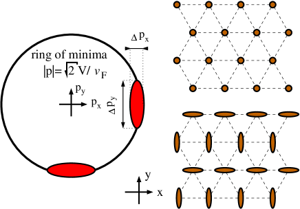
Figure 2: Visualization of the electronic density in a Wigner crystal with Mexican-hat shaped kinetic energy dispersion in the momentum(left) and coordinate(bottom-right) representation according to Ref. Silvestrov14 . Top-right - the Wigner crystal at the intermediate electron density, where fluctuations preserve the triangular lattice symmetries.

7. Conclusions.– Our main result in this paper is the prediction of the existence of Wigner crystalline phases in lightly doped bilayer graphene subject to an interlayer voltage. This is in contrast to single-layer graphene and bilayer graphene without a gap, where scaling arguments (together with screening properties for bilayer graphene) prove the absence of the crystallization Balatsky06 .

Moreover, we predict the existence of two distinct crystal phases at different electron densities, having different symmetries and are separated by a quantum phase transition. We suggest differential capacitance measurements for the experimental verification of the transition.

Further investigations of Wigner crystals with non-quadratic kinetic energy may be done numerically via the Quantum Monte Carlo method. At least for the case of the quartic energy dispersion, $\varepsilon\propto p^{4}$, this may be not more difficult than the standard calculation Tanatar89 ; Drumond09 .

The two phases of the Wigner crystal predicted in this paper exist if the voltage between the graphene layers is small compared to the interlayer coupling, $V\ll t_{\perp}$. Assuming $V=t_{\perp}/10$ we estimate from Eqs. (15, 16) the liquid-to-solid ($ls$) and the solid-to-solid ($ss$) transitions to appear at $a_{ls}\approx 23\,d$ and $a_{ss}\approx 720\,d$, or at the electron densities $n_{ls}\approx 1.1\cdot 10^{13}{\rm cm}^{-2}$ and $n_{ss}\approx 1.1\cdot 10^{10}{\rm cm}^{-2}$. We must mention however, that in the usual electron gas with parabolic dispersion consideration similar to ours overestimates the transition density by a large pure numerical factor Tanatar89 ; Drumond09 .

Concerning other effects potentially affecting the crystallization: Disorder may be ignored, since electron’s mean free path in bilayer graphene may be as large as micrometers Schoeneberger2015 . Temperature, to play a role, should be comparable to (e.g. kinetic) electron’s energy. For the low density solid-to-solid transition this gives $T\sim V^{3}/t_{\perp}^{2}\approx 5{\rm K}$ (for $V=t_{\perp}/10$). As usual EAndrey88 , a quantizing magnetic field will simplify the observation of a (Skyrme-)Wigner WignerMagnetic ; SkyrmeMagnetic crystal in bilayer graphene. However, the magnetic field will also destroy the low density crystal phase from Fig. 2.

I Appendix: Screening in gapped bilayer graphene

Here, we consider the static screening of the Coulomb interaction between electrons in intrinsic(undoped) bilayer graphene with an interlayer voltage. A detailed discussion of the interaction effects in graphene may be found e.g. in the review KotovRMP12 . However we are not aware of any publication emphasizing the absence of interaction corrections in the dielectric constant of gapped bilayer graphene and especially the existence of the intermediate regime for the interaction Eq. (37) for $V\ll t_{\perp}$.

The standard approach to screening of the electrostatic potential is by introducing the momentum dependent dielectric constant $\epsilon(q)$ via

$$U(q)=\frac{2\pi e^{2}}{\epsilon_{0}q}\ \rightarrow\ \frac{2\pi e^{2}}{\epsilon(q)q}\ .$$ (20)

Here, the bare dielectric constant $\epsilon_{0}$ for the case of exfoliated graphene on silicon-oxide is $\epsilon_{0}=(\epsilon_{{\rm SiO_{2}}}+1)/2$ SilvestrovPRB08 and $\epsilon_{SiO_{2}}\approx 4.2$. In suspended graphene obviously $\epsilon_{0}=1$. The dielectric function is usually calculated in the random phase approximation (RPA), yielding

$$\epsilon(q)=\epsilon_{0}[1-U(q)\Pi(q)]\ ,$$ (21)

where the polarization function $\Pi(q)$ is found in a single bubble approximation.

In order to have a finite dielectric constant at low momenta the polarization function should vanish at small $q$ as $\Pi(q\rightarrow 0)\sim q$. This indeed happens in a single layer graphene, where the static dielectric constant in the RPA approximation takes the form

$$U_{\rm RPA}=\frac{1}{\epsilon_{\rm RPA}}\frac{e^{2}}{r}\ ,\ \epsilon_{\rm RPA}=\frac{\epsilon_{{\rm SiO_{2}}}+1}{2}+\frac{\pi}{2}\frac{e^{2}}{\hbar v_{F}}\ .$$ (22)

For the case of bilayer graphene in the regime I of Eq. (7) of the main text one should simply double the interaction ($\sim e^{2}$) term in $\epsilon_{\rm RPA}$ (22) and use this formula for $r<\hbar\,v_{F}/t_{\perp}$.

The result Eq. (22) is already surprising. Graphene is only a two-dimensional sheet of atoms. How can it show the same effect on screening of a long-range interaction potential as a three-dimensional bulk of ${\rm SiO_{2}}$? This may happen only because graphene has no bandgap and consequently a much higher polarizability.

The situation is even more interesting in bilayer graphene. In the ungapped case the spectrum of the bilayer consists of two parabolic bands touching each other at the $K$ ($K^{\prime}$) point. This means that the density of states around the Fermi energy in intrinsic bilayer graphene is constant

$$\left.\frac{dn}{d\varepsilon}\right|_{\varepsilon\approx 0}=const\neq 0\ ,$$ (23)

similar to that in a usual two-dimensional metal. This results in an even larger polarizability than for single layer graphene, sufficient to develop a full screening of the electric charge, as was shown in the one-loop calculation in Ref. Hwang08 . In this case the polarization operator $\Pi(q)$ turns out to be a constant independent of $q$ and the interaction potential in the momentum representation Eq. (20) takes the form

$$U(q)=\frac{2\pi e^{2}}{\epsilon_{0}q}\rightarrow\frac{2\pi e^{2}}{\epsilon_{0}(q+q_{\rm TF})}\ ,$$ (24)

where the Thomas-Fermi screening wave vector is Hwang08

$$q_{\rm TF}=\frac{2t_{\perp}e^{2}}{\epsilon_{0}\hbar^{2}v_{F}^{2}}\ln 4\ .$$ (25)

The charge of the electron in Eq. (24) is fully compensated by the cloud of charges induced in graphene at a distance $\sim 1/q_{\rm TF}$. Since this is a two-dimensional charge cloud, the potential is not fully screened, but rather decays (in plane) as a power law $U(r\gg 1/q_{\rm TF})\sim 1/r^{3}$.

In bilayer graphene with an interlayer voltage $V$, described by the Hamiltonian Eq. (5), the result Eq. (24) is valid as long as one may neglect the gap $\sim V$ in the electron’s spectrum, i.e. at $q\gg\sqrt{Vt_{\perp}}/\hbar v_{F}$. For smaller momenta (larger distances between electrons) one should consider the graphene sheet as a narrow-gap two-dimensional insulator. The polarization function $\Pi(q)$ here decreases with decreasing $q$ as $\Pi(q)\sim q^{2}$ (see the calculation below). Eventually at very small $q$ the polarization function contribution to the dielectric constant becomes negligible, i.e. $\epsilon(q)=\epsilon_{0}$ in Eq. (20). This means that at largest distances the screening of the electron’s interaction is fully determined by the bulk three-dimensional dielectric below and above the graphene flake, $U(r\rightarrow\infty)=e^{2}/\epsilon_{0}r$. The transition from the fully screened, $U\sim 1/r^{3}$, to the unscreened Coulomb interaction does not happen instantaneously, but rather proceeds continuously in the parametrically wide region of inter-electron distances, $\hbar v_{F}/\sqrt{t_{\perp}V}\ll r\ll\hbar v_{F}/V$. Below we describe the behavior of the screened potential $U(r)$ at these intermediate distances.

To describe quantitatively the evolution of the electron’s interaction from the fully screened to the unscreened regime, we consider the calculation of the polarization function $\Pi(q)$. First we notice that the Thomas-Fermi screening Eq. (25) and transition between quadratic (II) and linear (I) spectrum regimes in Eq. (7) of the main text take place at the same momentum $\sim q_{\rm TF}$, since in graphene $e^{2}/(\hbar v_{F})\sim 1$. This means that we may use a simplified two-band Hamiltonian for a reliable description of the polarization, instead of the full four-band Hamiltonian Eq. (5), cf. Hwang08 ,

$${\cal H}_{eff}=\left(\begin{array}[]{cc}\ \ \ \ \ \ -V\ \ \ \ \ -{\tilde{p}}^{2}v_{F}^{2}/t_{\perp}\\ -{\tilde{p}}^{*2}v_{F}^{2}/t_{\perp}\ \ \ \ V\end{array}\right)\ ,$$ (28)

where ${\tilde{p}}=p_{x}+ip_{y}$. The two eigenvalues of the two-band Hamiltonian are

$$\varepsilon_{p\pm}=\pm\varepsilon_{p}\ ,\ \varepsilon_{p}=\sqrt{V^{2}+p^{4}v_{F}^{4}/t_{\perp}^{2}}\ ,$$ (29)

which reproduce correctly the spectrum of the four-band Hamiltonian Eq. (5) in the regimes II and III of Eq. (7). The lowest energy Mexican-hat spectrum, Eq. (7) regime IV, may be found only from the four-band model. However, as we will see, the two-band approximation Eq. (28) leads to the correct form of the polarization function $\Pi(q)$ even for the momentum transfer $q$ corresponding to the lowest energy regime IV in Eq. (7). The two positive- and negative-energy eigenfunctions of ${\cal H}_{eff}$ in Eq. (28) are

$$\psi_{+}=\frac{1}{\sqrt{{p}^{4}v_{F}^{4}/t_{\perp}^{2}+(V+\varepsilon_{p})^{2}}}\left(\begin{array}[]{cc}{\tilde{p}}^{2}v_{F}^{2}/t_{\perp}\\ -(V+\varepsilon_{p})\end{array}\right)\ ,$$ (30)

and

$$\psi_{-}=\frac{1}{\sqrt{{p}^{4}v_{F}^{4}/t_{\perp}^{2}+(V+\varepsilon_{p})^{2}}}\left(\begin{array}[]{cc}V+\varepsilon_{p}\\ {\tilde{p}}^{*2}v_{F}^{2}/t_{\perp}\end{array}\right)\ .$$ (31)

The zero temperature polarization function in the single bubble approximation may now be written as

$$\Pi(q)=-g\int\frac{d^{2}p}{(2\pi\hbar)^{2}}\left[\frac{|\psi_{+}^{\dagger}\psi_{-}^{\prime}|^{2}}{\varepsilon_{\mathbf{p}+}-\varepsilon_{\mathbf{p}^{\prime}-}}+\frac{|\psi_{+}^{\dagger}\psi_{-}^{\prime}|^{2}}{\varepsilon_{\mathbf{p}^{\prime}+}-\varepsilon_{\mathbf{p}-}}\right]\ .$$ (32)

Here $\hbar\mathbf{q}=\mathbf{p}-\mathbf{p}^{\prime}$, $\psi^{\prime}=\psi(p^{\prime})$ and the degeneracy factor $g=4$ accounts for two valleys and two spin orientations. For the gapless case, $V=0$, formulas for $\psi_{+}$ and $\psi_{-}$ are greatly simplified and Eq. (32) coincides with Eq. (4) of Ref. Hwang08 .

Moreover, in the case of vanishing $V$ the overlap of two eigenvectors depends only on the ratio $p/q$ and the angle between two momenta, $|\psi^{\dagger}_{+}\psi^{\prime}_{-}|^{2}=1-(\mathbf{p}\mathbf{p}^{\prime})^{2}/p^{2}p^{\prime 2}$, while the energy in this case is simply quadratic in momentum $\varepsilon_{\mathbf{p}\pm}\propto\pm p^{2}$. As a result the polarization function Eq. (32) in the limit $V=0$ turns out to be a constant independent of the momentum transfer $q$ Hwang08

$$\Pi(q)\approx\Pi_{V=0}=-\frac{\ln 4}{\pi}\frac{t_{\perp}}{\hbar^{2}v_{F}^{2}}\ ,$$ (33)

leading to the Thomas-Fermi screening Eqs. (24, 25).

The situation is different in the case of a finite interlayer voltage, $V\neq 0$, and a very small momentum transfer, $q\ll\sqrt{t_{\perp}V}/\hbar v_{F}$. The integral over momentum in this limit comes from the region $p\sim\sqrt{t_{\perp}V}/v_{F}$. This means that typically $p\gg q$ and the overlap of two different eigenfunctions of almost the same Hamiltonians, ${\cal H}_{eff}(p)$ and ${\cal H}_{eff}(p^{\prime})$ in Eq. (28), vanishes as $|\psi^{\dagger}_{+}\psi^{\prime}_{-}|^{2}\propto q^{2}$. This leads to the quadratic in small momentum transfer $q$ behavior of the polarization function (see Eqs. (38, 39) for the explicit calculation)

$$\Pi(q)=\frac{-2}{3\pi}\frac{q^{2}}{V}\ .$$ (34)

According to Eqs. (20, 21) this results in the absence of electron’s interaction contribution to the dielectric constant in gapped bilayer graphene at very large distances.

The fact that at low momentum transfer the $\sim q^{2}$ behavior of the polarization function Eq. (34) is due to the small overlap of the spinors $\psi^{\dagger}_{+}\psi_{-}^{\prime}\sim q$, while the nontrivial integration goes over the large-momentum region, $p\sim\sqrt{t_{\perp}V}/v_{F}$, suggests that this result may be valid also for very small values of $q$, where at $q\sim V/v_{F}$ the dispersion $\varepsilon(q)$ is described properly by the full four-band Hamiltonian Eq. (5). Indeed, in order to calculate the polarization function directly from the four-band Hamiltonian one would need to add in Eq. (32) a summation over the double set of $+$ and $-$ states, $\psi_{i\pm}$, and to modify the dispersion $\varepsilon(p)$ in Eq. (29) accordingly. However, also in this case, the product of two eigenvectors vanishes at small momentum transfer, $|\psi^{\dagger}_{i+}\psi_{j-}^{\prime}|\sim q$, leading to the $\sim q^{2}$ smallness of $\Pi(q)$. As a fact, the contribution to the remaining integral from the new terms added into Eq. (32) will be suppressed due to the larger denominators ($\sim t_{\perp}$ instead of $\sim V$). The modification of the term in $\Pi(q)$ describing the transitions between the two lower energy bands of the four-band model will also lead to corrections of the small relative order $\sim V/t_{\perp}$.

The result Eq. (34) reveals a nontrivial distribution of charges induced in bilayer graphene with an interlayer voltage. First, as we saw in Eqs. (24, 25), for the case of a very small gap $V$ the negative charge of an electron is compensated by the positive charge cloud at distances $\sim 1/q_{\rm TF}$. However, as we see in Eq. (34), the screening of the original electron charge starts to disappear at distances $\sim\hbar v_{F}/\sqrt{t_{\perp}V}$. This implies the existence of a second very large negative charge cloud restoring the original electron’s charge.

The low-momentum-transfer formula Eq. (34) is valid for $q\ll\sqrt{t_{\perp}V}/\hbar v_{F}$, when the polarization operator is small compared to the gapless case, $\Pi(q)\ll\Pi_{V=0}$. Interestingly, however, this does not imply that this ”small” polarization operator is not sufficient to modify strongly the electrons’ interaction. Indeed, combining Eqs. (20, 21, 34) we write

$$U(q)=\frac{2\pi e^{2}}{\epsilon_{0}q+q^{2}/q_{0}}\ ,$$ (35)

where $q_{0}=3V/(4e^{2})\sim V/(\hbar v_{F})$. This formula is still valid for $q\gg q_{0}$, where the second, interaction induced term in the denominator dominates.

The coordinate representation of the interaction Eq. (35) is found via the standard Fourier transformation. The essential part of the calculation of $U(r)$ reduces then to find the integral GradshteynRyzhik

$$\int_{0}^{\infty}\frac{J_{0}(k)dk}{x}=\frac{\pi}{2}[H_{0}(x)-N_{0}(x)]\ ,$$ (36)

where $x=\epsilon_{0}q_{0}r$ and $J_{0},N_{0},H_{0}$ are the Bessel, Neumann and Struve functions, resp. For $\hbar v_{F}/\sqrt{t_{\perp}V}\ll r\ll\hbar v_{F}/V$ this gives

$$U(r)\approx\frac{3V}{4}\ln\left(\frac{\hbar v_{F}}{rV}\right)\ .$$ (37)

At larger distances, the potential Eq. (37) crosses over into the usual Coulomb potential $U(r)=e^{2}/\epsilon_{0}r$, while at shorter distances it transforms into $U(r)\approx e^{2}/\epsilon_{0}r(q_{\rm TF}r)^{2}$, which is the screened interaction in bilayer graphene without a gap Hwang08 .

II Derivation of Eq. (34)

A straightforward calculation of the overlap of the two spinors in Eqs. (30, 31) to leading order in small $q$ gives

$$|\psi_{+}^{\dagger}\psi_{-}^{\prime}|^{2}=\frac{4}{[p^{4}+(V+\varepsilon)^{2}]^{2}}$$ (38)

$$\times\left[p^{2}q^{2}(V+\varepsilon)^{2}-2\frac{(\mathbf{p}\mathbf{q})^{2}p^{4}(V+\varepsilon)}{\varepsilon}+\frac{(\mathbf{p}\mathbf{q})^{2}p^{8}}{\varepsilon^{2}}\right].$$

Here, for a moment, we set $\hbar=t_{\perp}=v_{F}=1$. Substitution of this into Eq. (32) followed by the angle integration and changing variables from $p$ to $x=p^{4}v_{F}^{4}/(t_{\perp}^{2}V^{2})$ leads to

$$\Pi(q)=\frac{-g}{2\pi}\frac{q^{2}}{V}\int_{0}^{\infty}\frac{e^{2}(1+e)^{2}-xe(1+e)+x^{2}/2}{e^{3}[(1+e)^{2}+x]^{2}}dx\ ,$$ (39)

where $e=\sqrt{1+x}$. Changing the integration variable from $dx$ to $de$ we now find

$$\Pi(q)=\frac{-g}{6\pi}\frac{q^{2}}{V}\ .$$ (40)