Type II supernovae progenitor and ejecta properties from the total emitted light,
Abstract
It was recently shown that the bolometric light curves of type II supernovae (SNe) allow an accurate and robust measurement of the product of the radiation energy in the ejecta, , and the time since the explosion, , at early phases () of the homologous expansion. This observable, denoted here is constant during that time and depends only on the progenitor structure and explosion energy. We use a 1D hydrodynamic code to find of simulated explosions of 145 red supergiant progenitors obtained using the stellar evolution code MESA, and relate this observable to the properties of the progenitor and the explosion energy. We show that probes only the properties of the envelope (velocity, mass and initial structure), similarly to other observables that rely on the photospheric phase emission. Nevertheless, for explosions where the envelope dominates the ejected mass, , is directly related to the explosion energy and ejected mass through the relation , where is the progenitor radius, to an accuracy better than . We also provide relations between and the envelope properties that are accurate (to within 20%) for all the progenitors in our sample, including those that lost most of their envelope. We show that when the envelope velocity can be reasonably measured by line shifts in observed spectra, the envelope is directly constrained from the bolometric light curve (independent of ). We use that to compare observations of 11 SNe with measured and envelope velocity to our sample of numerical progenitors. This comparison suggests that many SNe progenitors have radii that are . In the framework of our simulations this indicates, most likely, a rather high value of the mixing length parameter.
Subject headings:
Type II supernovae1. Introduction
The most common type of supernovae (SNe) are type II supernovae (supernovae with spectra showing significant amounts of hydrogen) and yet it is still unclear how these explosions work. While several lines of evidence indicate that the explosion is associated with the latest stages of stellar evolution of some massive stars and the collapse of their cores, the process in which the envelope is energetically ejected is poorly understood.
Recent extensive surveys and followup efforts are leading to the accumulation of large samples of well observed type II SNe. Given the diversity in the observed properties (e.g. peak luminosity), statistical inferences are likely to play an important role in improving our understanding of these events. Most observations of SNe in general, and type II in particular, consist of spectra and light curves of visible light acquired throughout weeks and months following the explosion. In order to connect the observed emission to the physical characteristics of the explosion and the progenitor star, studies usually either employ detailed radiation transfer calculations or use simplistic analytic models. While the former are more trustworthy, they are difficult to apply to the growing large samples of observed SNe, especially given the uncertainty in the late phase structure of the massive stars which are likely the progenitors. The application of simplistic analytic models is useful but may lead to crude errors in estimates of the interesting properties such as explosion energy, mass and radius of the progenitor.
Recently, we showed (Nakar et al., 2015; Katz et al., 2013) that the bolometric light curve can be used to extract information on the explosion which circumvents the difficulty of radiation transfer by direct use of energy conservation. For that we defined a time-weighted integrated luminosity (with the 56Ni contribution subtracted) which is directly observable. We denoted it and in Nakar et al. (2015) measured it for a sample of 13 SNe. is set by the energetics of the explosion and the structure of the progenitor and it provides a direct relation between observations and explosion models which is simple, analytic and precise at the same time.
The purpose of this paper is to use hydrodynamic simulations to study the relation between this measurable quantity and useful parameters of the progenitor and explosion. To do that we calculate ET for a large set of 145 red supergiant models that are obtained by the stellar evolution code MESA (Paxton et al., 2011, 2013, 2015) by varying progenitor parameters on the main sequence (initial mass, metallicity and rotation) and an evolution parameter (mixing length parameter).
The paper is organized as follows. In section §2 we briefly repeat the arguments of Nakar et al. (2015) and Katz et al. (2013), and explain how the total radiation energy can be measured and how exactly it is connected to the hydrodynamic properties of the explosion. In section §3 we describe the set of numerical progenitors we use and present the relations we find between and fundamental properties of the progenitor and explosion energy. In section §4 we use observations of SNe with measured ET and envelope velocity to constrain the envelope mass and radius, and SNe with measured ET, envelope velocity and pre-explosion radius to constrain the explosion energy.
2. is measurable, independent of radiation transfer, and scales as
We first briefly repeat the arguments of Nakar et al. (2015) and Katz et al. (2013). During the time span of about 1 to 10 days after the explosion, the expansion is homologous and the radiation is almost entirely trapped within the ejecta. In addition, the contribution of energy from the decay of 56Ni is negligible. The total energy in radiation , originating from the explosion shock wave, decreases with time adiabatically due to the work it does on the expanding ejecta. To a very good approximation it decreases in this phase as where is the time since explosion and thus we define
| (1) |
which is constant with time. Since there is negligible diffusion during this time, the quantity is completely set by the hydrodynamic properties of the explosion and is independent of the opacity of the ejecta. At later times diffusion becomes important and the trapped internal energy leaks out of the ejecta gradually to generate the observed luminosity. Thus, as shown by Nakar et al. (2015), by integrating over the observed bolometric luminosity (multiplied by to compensate for adiabatic losses), and removing the contribution from 56Ni, one can directly extract from observations.
To show that formally we start from the equation that describes the radiation energy which is trapped in the ejecta during the homologous phase:
| (2) |
Here, is the energy injection rate from 56Ni decay and is the bolometric luminosity. The term is the total rate of adiabatic loss. After rearranging the equation, multiplying both sides by and integrating over in some interval we obtain
| (3) |
By choosing to be in the range , we can replace in equation 3 by . By choosing that is large enough (typically d) so the diffusion time is shorter than the expansion time and the remaining radiation in the ejecta is negligible, we can neglect the term . Finally, since the (time weighted) integrated luminosity at early times is negligible, we can extend the integration from without affecting the result. We therefore find
| (4) |
The second term on the RHS of equation 4 can be calculated using
| (5) |
where d and is the 56Ni mass ejected in the explosion. can be accurately inferred from the amplitude of the bolometric luminosity at late times where to a very good approximation
| (6) |
(at later times -ray escape may become significant). The value of can thus be directly extracted from observations of type II SNe using equations 4 - 6, as long as the bolometric luminosity is measured up to the 56Ni tail phase (where ).
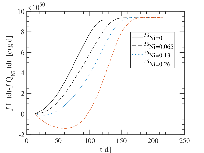
We note that is also equal to the (time weighted) integrated ’cooling envelope luminosity’ defined as the luminosity that would have been generated if there was no 56Ni present in the ejecta
| (7) |
Equation 7 is useful for studying the different approximations in radiation transfer simulations were the 56Ni can be artificially extracted. This is demonstrated in figure 1 using the results of radiation transfer simulations reported in (Kasen & Woosley, 2009).
We next derive the scaling we expect for with the progenitor radius, , ejecta mass, , and total explosion energy, . In this paper we ignore the inner collapsing parts of the progenitor and the initial thermal and gravitational energy which is negligible when considering the material at large radii (). The explosion is thus described as a shock wave traversing a cold standing star and a following expansion. While the shock is within the star, there is negligible diffusion and the thermal energy is dominated by radiation. Thus, for a set of progenitors with the same density profile111Two progenitors, denoted as ’1’ and ’2’, have the same density profile if , where is density, is the progenitor mass and , by the time the shock ends traversing the star and breaks out the radiation energy contained in the ejecta is and the expansion time over which significant adiabatic losses take place is . Thus for progenitors with similar profiles scales as
| (8) |
where
| (9) |
is the (mass weighted) RMS velocity of the ejecta ( is the velocity of the mass element ). However, since stars with different initial conditions (e.g., ZAMS mass, metallicity, rotation, binarity, etc.) have different density profiles before they explode, the coefficient in equation 8 for each progenitor structure is expected to be different. Below we calculate for a large set of progenitors and find the typical value of the coefficient and how it varies between different progenitors. We also study which of the progenitor and explosion properties can be constrained best by measuring .
3. Numerical study of the scaling of with progenitor parameters
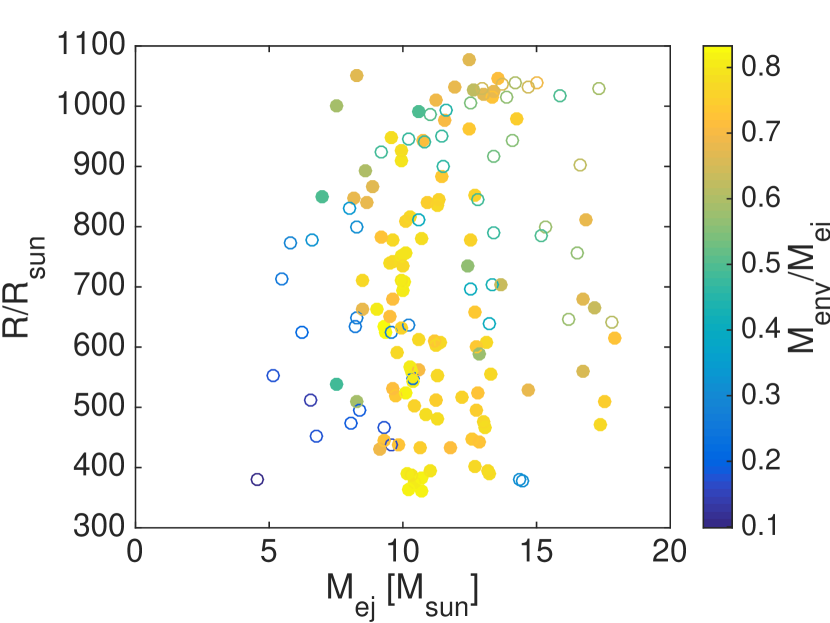
We have used the open source stellar evolution code MESA (Paxton et al., 2011, 2013, 2015) to calculate a large set of progenitors. Only single star evolution is considered (no binarity) and three initial conditions are varied - initial (ZAMS) mass (12-50 ), metallicity () and initial rotation (0-0.8 of breakup rotation rate). We have also varied one poorly constrained evolution parameter - the mixing length parameter (1.5-5). Altogether we calculate the stellar structure at the time of core collapse for 219 stars. Out of these 145 retain a hydrogen envelope at the time of explosion and are therefore considered here as plausible progenitors of type II SNe. Figure 2 depicts some of the main properties of these 145 progenitors. The evolution parameters, together with the main properties at explosion are given in table 2. More details on the set of progenitors we use here are given in Shussman et al. (2016)
In order to calculate for all the progenitors that retain hydrogen envelope, we excise the Si core from each progenitor (considered to be the explosion remnant), and explode it using a a simple 1D hydro-radiation code (see Shussman et al. 2016 for more details on the code). The explosion is induced by instantaneously releasing the explosion energy at the center of the ejecta. We then calculate , by extracting the asymptotic value of at late times ( d) using hydrodynamics alone, without allowing for radiation to diffuse. We have verified that the results remain unchanged when radiation transfer is included, in which case is calculated using equation 7. As explained above (equation 8) for a given progenitor we expect . We find that this is indeed the case in our simulations (to within 1%). Thus, as the dependence of on is known, we focus here on its dependence on the progenitor properties.
We first measure the coefficient of the scaling given in equation 8, in our progenitor sample. As can be seen in figure 3 for progenitors that retain most of their envelope, , the relation
| (10) |
is accurate to within about 30%. Such progenitors include almost all the models with initial mass that have a massive envelope (). Pre-explosion images of progenitors and light curve modeling of type II-P SNe (e.g., Smartt, 2015, and references therein) suggest that at least progenitors of this SN type fall into this category. Therefore equation 10 can be applied within fair accuracy to regular type II-P SNe.

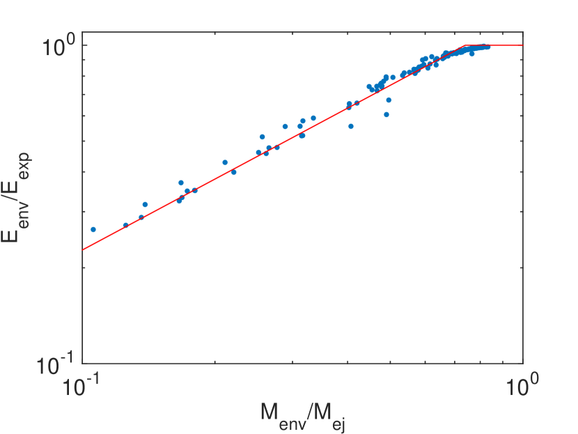
Figure 3 also shows that although equation 10 is rather accurate for progenitors with it becomes less accurate as the envelope mass fraction drops, becoming inaccurate by more than an order of magnitude for . To understand why low values of affect the scaling of equation 10 we recall that is proportional to the radiation energy at the beginning of the homologous phase and not directly to the total explosion energy. In progenitors with low most of the explosion energy is deposited in the core, but all the radiation energy deposited in the core is lost via adiabatic expansion well before the homologous phase. Only radiation energy deposited in the envelope remains by the beginning of the homologous phase. The total energy deposited in the envelope is roughly proportional to , as can be seen in figure 4. Thus, a low value of implies that a smaller fraction of the explosion energy contributes to .
In fact, the emission during the photospheric phase, after removing 56Ni contribution, is completely dominated by the radiation energy deposited in the envelope during the SN explosion (hence the term ‘cooling envelope emission’). Thus, , is actually a direct probe of the envelope properties and is not directly sensitive to properties of the core such as its mass or velocity. The same is true for any other probe that depends mostly on the cooling envelope emission (such as the photospheric velocity during the plateau, the plateau luminosity and duration, etc.). Therefore it is most useful to define scaling of that depends only on envelope properties:
| (11) |
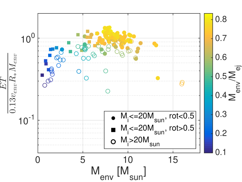
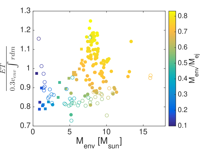
Here, is the energy carried by the envelope to infinity and is the envelope (mass weighted) RMS velocity. Figure 5 shows that indeed provides better estimates for global envelope properties than to those of the entire ejecta. Equation 11 provides a moderate improvement to progenitors that retain most of their envelope (), where it is accurate to within about 20% (the normalization of equation 11 was chosen to better match such progenitors). More importantly, equation 11 is applicable also to progenitors that lost most of their envelope, where it is accurate to within a factor of about 3.
So far we have ignored the density structure of the envelope, which of course also affects the value of . When crossing a mass element, the shock deposits half of its energy as kinetic and half as internal (i.e., radiation). The expansion (and adiabatic cooling) of the element begins right after the shock crossing. Thus, the fraction of the deposited energy that remains once the homologous phase starts depends on the initial radius of each mass element and not directly on . In both equations 10 and 11, is used as the envelope radius. However, explosions of two progenitors with similar , , and different density profiles will result in different values of . Specifically, will be lower in the progenitor that is more concentrated (i.e., most of its envelope mass is at a smaller radius). To account for that, one can attribute the initial radius to each mass element by replacing with the integral . Note that the value of this integral is insensitive to whether it is taken over the envelope mass alone or over the entire ejecta since it is completely dominated by mass elements at large radii. Using this integral we find
| (12) |
where
| (13) |
is the mass weighted average radius of the envelope. Equation 12 is accurate to within about 20% to all the progenitors in our sample, as can be seen in Figure 6. Note that while hardly changes if the integral is performed over the entire progenitor including the core, does change due to the different mass in the denominator of equation 13.
4. supernovae with spectral measurement of the photospheric velocity
In many SNe spectral measurements provide information about the ejecta velocity. In particular for type II SNe, lines of Fe II and Sc II are considered to be good indicators of the photospheric velocity. In these SNe the photosphere crosses the H envelope from the outside in during the photospheric phase, providing a ‘scan’ of the envelope velocity range. The propagation of the photosphere at early time, before recombination becomes significant, depends only on the density and velocity profile of the ejecta and is relatively simple to model. Recombination becomes significant typically around day 20, when the photosphere has crossed only a very small fraction of the envelope (; see Shussman et al. 2016). The time at which the photosphere ends crossing the envelope is marked in type II SNe by a sharp drop in the luminosity and is observed typically around day 100. Thus, the photospheric velocity as measured around day 50, typically denoted , provides a reasonable estimate of . Moreover, since the photospheric velocity evolves roughly as (Nugent et al., 2006; Faran et al., 2014) it varies between day 20 and 100 by a factor of , implying that estimates to an accuracy of 50% at worst, and most likely much better.
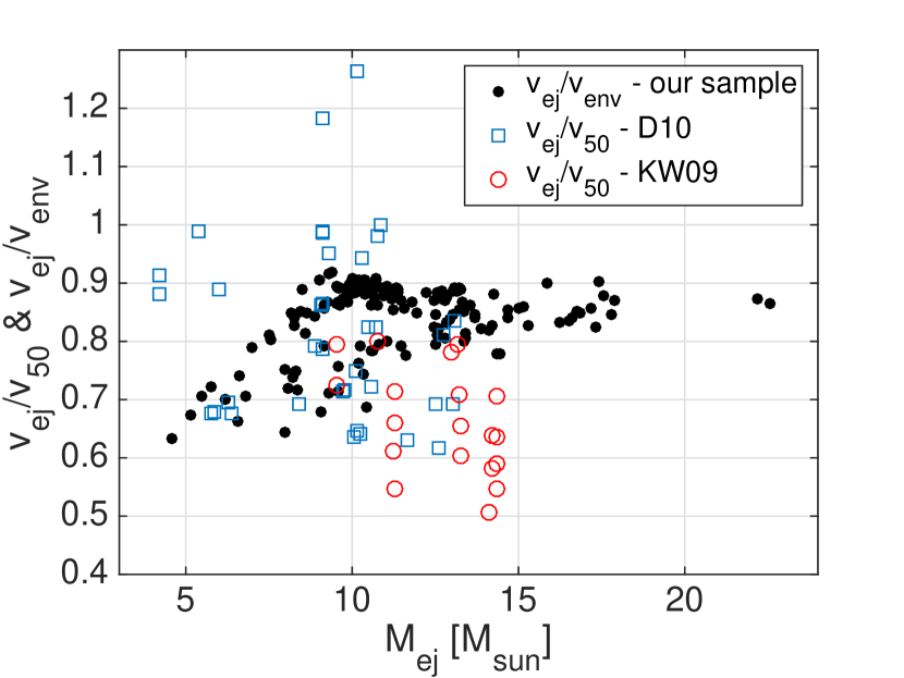
The quality of as an estimator of can also be estimated from numerical modeling of type II SN light curves. For that we use the results of Dessart et al. (2010) (table 2 therein) and Kasen & Woosley (2009) (table 2 therein). Both studies present a set of hydrodynamic numerical SNe simulations that include detailed radiative transfer to explore properties of various observables including . Unfortunately, these publications do not include the values of , but they do provide the values of . Figure 7 depicts in Dessart et al. (2010) and Kasen & Woosley (2009), showing that they find in general . It also shows the values of in our progenitor sample showing . Thus, the reasonable assumption that in our sample are similar to those of Dessart et al. (2010) and Kasen & Woosley (2009), implies that is a good estimator of and that at least in these simulations it is accurate to within about 25%.
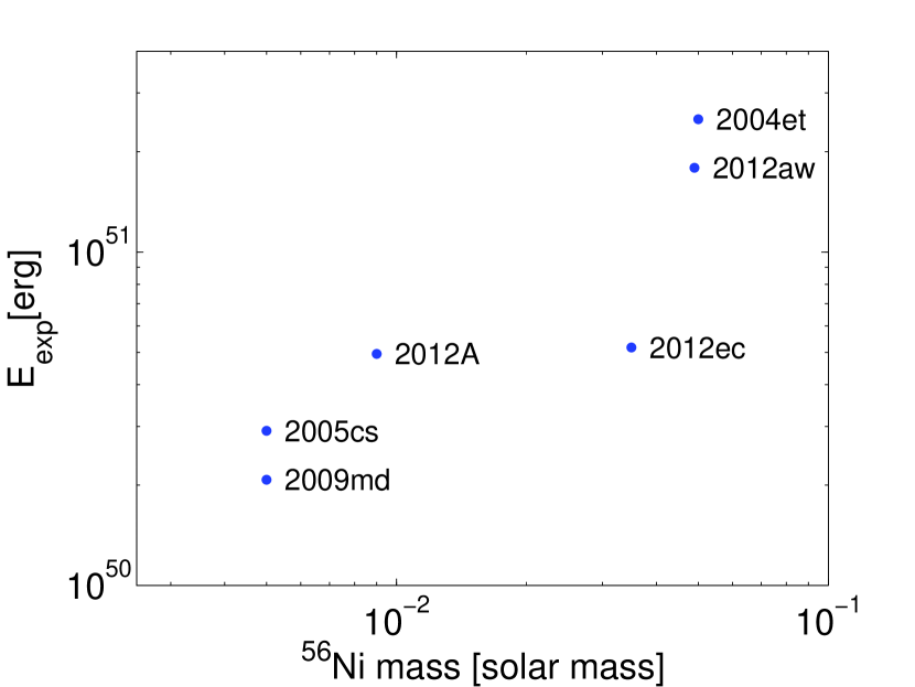
Therefore, in SNe where both and are measured we can estimate two interesting quantities based on equations 10 - 12. The first is which is an estimator of (or more accurately of ). This can be used, for example, to estimate the explosion energy in cases where there are pre-explosion images of the progenitor, which constrain . We have done that for six SNe for which , and are all measured independently (see table 1). Given that in all six the progenitor seems like normal red supergiants with initial masses (Smartt, 2015), equation 10 can probably be used to estimate within fair accuracy (within a factor of 2 given the large uncertainty in ). In figure 8 we depict , as estimated based on equation 10 for these six SNe, as a function of the 56Ni mass in the explosion. Even with that small number of SNe it is clear that varies by at least an order of magnitude between various SNe, and that SNe with erg are common (these SNe are also fainter and thus harder to detect, so their fraction of the total SNe volumetric rate is probably higher than their representation in the observed sample). In addition, a strong, roughly linear, correlation exists between and the 56Ni mass (Kushnir, 2015). This correlation is most likely the main source of the well known correlation between the plateau luminosity, and the 56Ni mass (Hamuy, 2003).
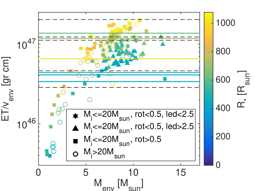
The second interesting quantity is which is an estimator of . The main advantage of is that it is a property of the progenitor, namely it depends only on the progenitor structure, with no dependence on the explosion energy. Thus, we can compare the observed values of to the values of in our sample of numerical progenitors. This comparison is shown in figure 9, which depicts the observed values of the 11 SNe listed in table 1 as horizontal lines, solid for SNe with pre-explosion progenitor images and dashed for SNe without. It also shows all the values for our numerical progenitors, which are divided to four groups, each marked differently, according to the initial conditions. It can be seen that numerical progenitors that lost most of their envelope () have that is lower than the observed ones. Almost all other numerical progenitors have within the observed range, but many are in the high end of that range ( gr cm) and few are in the low end ( gr cm). This is significant since half of the observed SNe in the sample have low values of and these are also the fainter ones, implying that they are most likely more abundant than their relative fraction in the sample.
A lower value of implies a lower value of . In our numerical sample there are two groups for which is relatively small. One is the group of stars with small , which had lost a significant fraction of their envelope, either via fast rotation ( of breakout velocity at birth) or due to a high initial mass (). However, this group does not seem to be the main origin of the observed low SNe. The reason for that is that high initial mass progenitors are not common (in all the cases where a progenitor was observed directly its mass was ; Smartt 2015). Rotation, on the other hand, seems to need a fine tuning in order to lose just the correct amount of envelope mass (most of the fast rotating models lost too much of their mass while others did not lose enough). The second group of low progenitors are stars with smaller () due to a larger value of the mixing length parameter ( or ). Given the uncertainty in the value of this coefficient we consider this option as the more likely explanation for the large number of low SNe. This option is also supported by the measured radii of progenitors observed in pre-explosion images, where the three SNe with in our sample with pre-explosion images have . The result that many SNe progenitors have radii that are is also supported by other, independent lines of evidence (Dessart et al., 2013; Davies et al., 2013; Gall et al., 2015; González-Gaitán et al., 2015)
| SN | Ref. | ||||
|---|---|---|---|---|---|
| [] | [km/s] | [] | [] | ||
| 1999em | 4 | 3280 | 14 | 1 | |
| 1999gi | 4.1 | 3700 | 16 | 1,2 | |
| 2004et | 5.5 | 4020 | 23 | 635 | 3 |
| 2005cs | 0.86 | 1980 | 1.9 | 420 | 4 |
| 2007od | 6.4 | 3130 | 32 | 5 | |
| 2009N | 1.2 | 2580 | 4.6 | 6 | |
| 2009ib | 0.88 | 3090 | 5.2 | 7 | |
| 2009md | 0.68 | 2000 | 2.4 | 471 | 8 |
| 2012A | 1.2 | 2840 | 6.1 | 516 | 9 |
| 2012aw | 4.6 | 3890 | 16 | 713 | 10 |
| 2012ec | 2.2 | 3370 | 10 | 1031 | 11 |
5. Conclusions
We have used a large set of 145 numerical stars, calculated to the point of core collapse using the stellar evolution code MESA, in order to study the relation between the observable and SN progenitors. can be measured for any SN with observed bolometric light curve. It is a time weighted integral of the cooling envelope emission, with radioactive contribution removed, and it measures the amount of radiation energy that is deposited in the envelope at the beginning of the homologous phase. As such it constrains directly the structure of the progenitor and the explosion energy, without any dependence on radiation transfer physics or on the contribution of radioactive decay to the observed light.
We have found that although depends on the exact structure of the progenitor, it is an accurate probe of for progenitors that retain most of the hydrogen envelope (equation 10). Specifically in our progenitor sample it is accurate to within for progenitors with . However, it is not an accurate probe of and for progenitors that lost most of their envelope, since is sensitive only to the fraction of the total energy that is deposited in the envelope, and this fraction is highly dependent on . We note that any observable which depends on the photospheric phase of type II SNe (e.g., plateau luminosity and duration), is sensitive mostly to envelope properties and is therefore, similarly to , only an approximate probe of the entire ejecta properties.
We have then explored how accurately can be related to envelope properties and found that it is a good probe of (equation 11). In our progenitor sample it is accurate to within for progenitors with and up to a factor of three for progenitors that lost most of their envelope. The dependence on the envelope mass arises from the fact that progenitors that lost different fractions of their envelope mass have different density structures. We therefore consider a third combination of properties which takes the envelope structure into account, , where is the mass weighted average radius of the envelope. In our sample measures to within accuracy for all progenitors, regardless of their envelope mass.
When the bolometric light curve is accompanied by spectral measurements of line velocities then both and can be estimated (as we have showed, provides a good estimate for ). This is very useful. First, the product is a probe of . We have used that in stars where was measured from pre-explosion images to estimate in a robust way which is insensitive to detailed and uncertain light curve modeling. Second, the ratio depends on the progenitor structure only, and is independent of the explosion energy. We have compared this quantity as measured in 11 SNe to that of our sample of numerical progenitors. This comparison suggests that SNe progenitors often have a radius , which is smaller than the typical RSG radius obtained by stellar evolution models. This result supports previous studies that got to the same conclusion based on completely different arguments (Dessart et al., 2010; Davies et al., 2013; González-Gaitán et al., 2015; Gall et al., 2015). Our simulations suggest that the small radii hint to relatively large values (3-5) of the mixing length parameter, as models with these values produce SNe with that is more similar to the observations.
| Initial parameters and properties of the numerical progenitors 11 | 0.02 | 2 | 0.4 | 10.07 | 9.72 | 7.19 | 518 | 225 | 0.97 | 2.34 |
| 12 | 0.0002 | 1.5 | 0 | 12.94 | 11.39 | 8.82 | 608 | 280 | 0.98 | 3.76 |
| 12 | 0.0002 | 1.5 | 0.2 | 12.89 | 11.27 | 8.72 | 603 | 271 | 0.98 | 3.56 |
| 12 | 0.0002 | 2 | 0 | 12.93 | 11.31 | 8.80 | 553 | 237 | 0.98 | 3.19 |
| 12 | 0.0002 | 2 | 0.2 | 12.88 | 11.28 | 8.68 | 552 | 230 | 0.98 | 2.99 |
| 12 | 0.0002 | 2 | 0.4 | 12.89 | 11.19 | 8.25 | 609 | 262 | 0.97 | 3.16 |
| 12 | 0.0002 | 3 | 0 | 12.94 | 11.31 | 8.85 | 480 | 193 | 0.98 | 2.63 |
| 12 | 0.0002 | 3 | 0.2 | 12.93 | 11.25 | 8.54 | 512 | 205 | 0.97 | 2.63 |
| 12 | 0.0002 | 3 | 0.4 | 12.89 | 11.25 | 8.46 | 511 | 200 | 0.97 | 2.51 |
| 12 | 0.002 | 1.5 | 0 | 11.59 | 10.02 | 7.70 | 736 | 353 | 0.98 | 4.43 |
| 12 | 0.002 | 1.5 | 0.2 | 10.49 | 8.86 | 5.94 | 867 | 438 | 0.95 | 4.09 |
| 12 | 0.002 | 1.5 | 0.4 | 10.80 | 9.17 | 6.60 | 783 | 379 | 0.97 | 4.10 |
| 12 | 0.002 | 2 | 0 | 12.23 | 10.59 | 8.20 | 614 | 270 | 0.98 | 3.51 |
| 12 | 0.002 | 2 | 0.2 | 11.60 | 9.94 | 7.49 | 633 | 279 | 0.97 | 3.35 |
| 12 | 0.002 | 2 | 0.4 | 11.32 | 9.64 | 6.86 | 681 | 298 | 0.96 | 3.16 |
| 12 | 0.002 | 3 | 0 | 12.48 | 10.85 | 8.47 | 489 | 198 | 0.98 | 2.63 |
| 12 | 0.002 | 3 | 0.2 | 11.98 | 10.41 | 7.85 | 502 | 201 | 0.97 | 2.48 |
| 12 | 0.002 | 3 | 0.4 | 11.25 | 9.60 | 6.89 | 532 | 210 | 0.96 | 2.29 |
| 12 | 0.002 | 5 | 0 | 12.66 | 11.02 | 8.72 | 396 | 153 | 0.99 | 2.12 |
| 12 | 0.002 | 5 | 0.2 | 11.48 | 9.86 | 7.12 | 438 | 161 | 0.96 | 1.82 |
| 12 | 0.002 | 5 | 0.4 | 12.23 | 10.65 | 7.90 | 432 | 161 | 0.97 | 1.96 |
| 12 | 0.02 | 1.5 | 0 | 11.51 | 9.97 | 7.93 | 910 | 454 | 0.98 | 6.22 |
| 12 | 0.02 | 1.5 | 0.2 | 11.36 | 9.93 | 7.74 | 926 | 466 | 0.98 | 6.13 |
| 12 | 0.02 | 1.5 | 0.4 | 11.16 | 9.59 | 7.45 | 948 | 481 | 0.98 | 6.20 |
| 12 | 0.02 | 1.5 | 0.6 | 9.93 | 8.26 | 5.52 | 1052 | 563 | 0.95 | 5.27 |
| 12 | 0.02 | 2 | 0 | 11.70 | 10.07 | 8.08 | 709 | 319 | 0.98 | 4.30 |
| 12 | 0.02 | 2 | 0.2 | 11.49 | 9.92 | 7.84 | 752 | 337 | 0.98 | 4.47 |
| 12 | 0.02 | 2 | 0.4 | 11.23 | 9.65 | 7.48 | 778 | 350 | 0.98 | 4.38 |
| 12 | 0.02 | 2 | 0.6 | 10.29 | 8.65 | 5.84 | 841 | 387 | 0.94 | 3.66 |
| 12 | 0.02 | 2 | 0.8 | 7.41 | 5.49 | 1.41 | 714 | 278 | 0.52 | 0.80 |
| 12 | 0.02 | 3 | 0 | 11.92 | 10.34 | 8.36 | 559 | 229 | 0.99 | 3.22 |
| 12 | 0.02 | 3 | 0.2 | 11.86 | 10.27 | 8.23 | 568 | 232 | 0.99 | 3.19 |
| 12 | 0.02 | 3 | 0.4 | 11.41 | 9.81 | 7.60 | 592 | 238 | 0.98 | 3.00 |
| 12 | 0.02 | 3 | 0.6 | 11.19 | 9.53 | 6.78 | 650 | 253 | 0.95 | 2.74 |
| 12 | 0.02 | 3 | 0.8 | 7.16 | 5.17 | 0.87 | 553 | 160 | 0.37 | 0.30 |
| 12 | 0.02 | 5 | 0 | 12.27 | 10.70 | 8.70 | 383 | 149 | 0.99 | 2.16 |
| 12 | 0.02 | 5 | 0.2 | 11.87 | 10.31 | 8.19 | 388 | 148 | 0.99 | 2.07 |
| 12 | 0.02 | 5 | 0.4 | 11.78 | 10.16 | 8.11 | 390 | 149 | 0.99 | 2.08 |
| 12 | 0.02 | 5 | 0.6 | 11.00 | 9.27 | 6.66 | 445 | 159 | 0.96 | 1.75 |
| 12 | 0.02 | 5 | 0.8 | 10.08 | 8.27 | 4.87 | 510 | 166 | 0.86 | 1.35 |
| 13 | 0.02 | 2 | 0 | 11.71 | 10.00 | 8.11 | 708 | 318 | 0.98 | 4.37 |
| 13 | 0.02 | 2 | 0.2 | 11.56 | 9.95 | 7.91 | 711 | 318 | 0.98 | 4.17 |
| 13 | 0.02 | 2 | 0.4 | 11.26 | 9.53 | 7.48 | 739 | 333 | 0.98 | 4.13 |
| 13 | 0.02 | 2 | 0.6 | 10.01 | 8.18 | 5.50 | 847 | 389 | 0.93 | 3.56 |
| 14 | 0.02 | 2 | 0 | 12.34 | 10.68 | 8.33 | 780 | 354 | 0.98 | 4.55 |
| 14 | 0.02 | 2 | 0.2 | 12.04 | 10.28 | 7.89 | 817 | 375 | 0.97 | 4.66 |
| 14 | 0.02 | 2 | 0.6 | 8.94 | 6.98 | 3.41 | 851 | 380 | 0.79 | 2.21 |
| 15 | 2e-05 | 1.5 | 0 | 14.98 | 13.27 | 10.29 | 555 | 247 | 0.98 | 3.44 |
| 15 | 2e-05 | 1.5 | 0.4 | 14.76 | 12.74 | 9.40 | 601 | 250 | 0.96 | 3.03 |
| 15 | 2e-05 | 3 | 0 | 14.97 | 13.07 | 10.18 | 465 | 182 | 0.98 | 2.51 |
| 15 | 2e-05 | 3 | 0.4 | 14.91 | 12.77 | 9.59 | 496 | 188 | 0.97 | 2.41 |
| 15 | 2e-05 | 5 | 0 | 14.98 | 13.22 | 10.30 | 390 | 146 | 0.98 | 2.05 |
| 15 | 2e-05 | 5 | 0.4 | 14.90 | 12.85 | 9.35 | 442 | 152 | 0.95 | 1.84 |
| 15 | 0.0002 | 1.5 | 0 | 14.95 | 13.10 | 10.13 | 608 | 277 | 0.98 | 3.82 |
| 15 | 0.0002 | 1.5 | 0.4 | 14.77 | 12.70 | 9.40 | 658 | 295 | 0.97 | 3.65 |
| 15 | 0.0002 | 3 | 0 | 14.92 | 13.02 | 10.02 | 476 | 188 | 0.98 | 2.55 |
| 15 | 0.0002 | 3 | 0.4 | 14.83 | 12.79 | 9.29 | 524 | 201 | 0.96 | 2.46 |
| 15 | 0.0002 | 5 | 0 | 14.93 | 13.16 | 10.14 | 394 | 149 | 0.98 | 2.06 |
| 15 | 0.0002 | 5 | 0.4 | 14.79 | 12.60 | 9.27 | 448 | 161 | 0.96 | 1.97 |
| 15 | 0.002 | 1.5 | 0 | 14.27 | 12.53 | 9.56 | 778 | 376 | 0.98 | 5.02 |
| 15 | 0.002 | 1.5 | 0.4 | 10.37 | 8.62 | 5.18 | 894 | 466 | 0.91 | 3.69 |
| 15 | 0.002 | 3 | 0 | 14.10 | 12.21 | 9.28 | 518 | 207 | 0.97 | 2.68 |
| 15 | 0.002 | 3 | 0.4 | 12.62 | 10.58 | 7.41 | 562 | 219 | 0.94 | 2.33 |
| 15 | 0.002 | 5 | 0 | 14.44 | 12.68 | 9.69 | 401 | 152 | 0.98 | 2.03 |
| 15 | 0.002 | 5 | 0.4 | 13.63 | 11.79 | 8.45 | 432 | 158 | 0.95 | 1.84 |
| 15 | 0.02 | 2 | 0 | 13.05 | 11.27 | 8.68 | 835 | 382 | 0.97 | 4.91 |
| 15 | 0.02 | 2 | 0.2 | 12.66 | 10.94 | 8.17 | 841 | 383 | 0.97 | 4.57 |
| 15 | 0.02 | 2 | 0.4 | 13.15 | 11.37 | 8.60 | 845 | 385 | 0.97 | 4.77 |
| 15 | 0.02 | 2 | 0.6 | 7.84 | 5.77 | 1.67 | 773 | 314 | 0.56 | 1.00 |
| 16 | 0.02 | 2 | 0 | 14.47 | 12.68 | 9.67 | 851 | 385 | 0.97 | 5.05 |
| 16 | 0.02 | 2 | 0.2 | 13.25 | 11.47 | 8.38 | 883 | 404 | 0.96 | 4.70 |
| 16 | 0.02 | 2 | 0.4 | 12.71 | 10.78 | 7.66 | 943 | 440 | 0.96 | 4.69 |
| 16 | 0.02 | 2 | 0.6 | 8.62 | 6.62 | 2.10 | 777 | 313 | 0.58 | 1.19 |
| 17 | 0.02 | 2 | 0 | 14.25 | 12.47 | 9.10 | 963 | 451 | 0.96 | 5.43 |
| 17 | 0.02 | 2 | 0.2 | 13.44 | 11.59 | 8.07 | 977 | 456 | 0.95 | 4.87 |
| 17 | 0.02 | 2 | 0.4 | 13.19 | 11.25 | 7.73 | 1009 | 480 | 0.94 | 4.96 |
| 17 | 0.02 | 2 | 0.6 | 8.50 | 6.20 | 1.31 | 625 | 208 | 0.43 | 0.53 |
| 18 | 0.02 | 2 | 0 | 16.25 | 14.23 | 10.67 | 978 | 451 | 0.97 | 5.98 |
| 18 | 0.02 | 2 | 0.2 | 15.22 | 13.32 | 9.61 | 1015 | 478 | 0.96 | 5.78 |
| 18 | 0.02 | 2 | 0.4 | 13.89 | 11.93 | 8.06 | 1031 | 489 | 0.94 | 5.06 |
| 18 | 0.02 | 2 | 0.6 | 8.58 | 6.57 | 0.91 | 512 | 131 | 0.32 | 0.24 |
| 19 | 0.02 | 2 | 0 | 15.46 | 13.53 | 9.58 | 1046 | 491 | 0.95 | 5.78 |
| 19 | 0.02 | 2 | 0.2 | 14.47 | 12.50 | 8.34 | 1077 | 509 | 0.93 | 5.23 |
| 19 | 0.02 | 2 | 0.6 | 9.42 | 6.78 | 1.17 | 452 | 90 | 0.35 | 0.22 |
| 20 | 2e-05 | 3 | 0.4 | 17.88 | 17.17 | 10.91 | 666 | 187 | 0.87 | 2.08 |
| 20 | 0.0002 | 1.5 | 0 | 19.94 | 17.41 | 13.33 | 471 | 58 | 0.94 | 0.98 |
| 20 | 0.0002 | 1.5 | 0.4 | 19.48 | 16.86 | 11.38 | 812 | 349 | 0.94 | 4.18 |
| 20 | 0.0002 | 3 | 0 | 19.91 | 17.90 | 12.93 | 616 | 238 | 0.96 | 3.35 |
| 20 | 0.0002 | 3 | 0.4 | 19.45 | 16.76 | 11.12 | 680 | 245 | 0.92 | 2.92 |
| 20 | 0.0002 | 5 | 0 | 19.92 | 17.57 | 13.11 | 511 | 185 | 0.97 | 2.71 |
| 20 | 0.0002 | 5 | 0.4 | 19.38 | 16.76 | 11.02 | 561 | 184 | 0.91 | 2.19 |
| 20 | 0.002 | 1.5 | 0 | 14.69 | 12.62 | 7.83 | 1027 | 522 | 0.92 | 4.74 |
| 20 | 0.002 | 1.5 | 0.4 | 12.73 | 10.59 | 5.18 | 991 | 472 | 0.80 | 3.05 |
| 20 | 0.002 | 3 | 0 | 15.70 | 13.67 | 8.65 | 703 | 271 | 0.90 | 2.76 |
| 20 | 0.002 | 3 | 0.4 | 14.72 | 12.44 | 7.04 | 735 | 271 | 0.83 | 2.36 |
| 20 | 0.002 | 5 | 0 | 16.70 | 14.69 | 9.94 | 529 | 186 | 0.92 | 2.20 |
| 20 | 0.02 | 2 | 0 | 15.41 | 13.38 | 9.11 | 1025 | 472 | 0.94 | 5.18 |
| 20 | 0.02 | 2 | 0.2 | 15.00 | 13.02 | 8.63 | 1019 | 469 | 0.93 | 4.91 |
| 20 | 0.02 | 2 | 0.4 | 10.10 | 8.00 | 2.68 | 830 | 325 | 0.59 | 1.39 |
| 21 | 0.02 | 2 | 0 | 15.74 | 13.70 | 9.04 | 1037 | 465 | 0.92 | 4.90 |
| 21 | 0.02 | 2 | 0.2 | 14.98 | 12.95 | 8.26 | 1030 | 461 | 0.91 | 4.63 |
| 21 | 0.02 | 2 | 0.4 | 11.47 | 9.18 | 4.43 | 925 | 389 | 0.77 | 2.44 |
| 22 | 0.02 | 2 | 0 | 17.37 | 15.01 | 10.36 | 1039 | 456 | 0.94 | 5.33 |
| 22 | 0.02 | 2 | 0.2 | 10.56 | 8.29 | 2.59 | 799 | 283 | 0.56 | 1.17 |
| 22 | 0.02 | 2 | 0.4 | 12.31 | 10.23 | 4.88 | 945 | 392 | 0.76 | 2.55 |
| 22 | 0.02 | 2 | 0.6 | 10.73 | 8.07 | 1.45 | 473 | 92 | 0.35 | 0.25 |
| 23 | 0.02 | 2 | 0 | 16.80 | 14.70 | 9.40 | 1032 | 442 | 0.90 | 4.65 |
| 23 | 0.02 | 2 | 0.2 | 13.09 | 11.04 | 5.60 | 986 | 417 | 0.79 | 3.01 |
| 23 | 0.02 | 2 | 0.4 | 12.94 | 10.80 | 5.13 | 942 | 380 | 0.75 | 2.54 |
| 23 | 0.02 | 2 | 0.6 | 10.49 | 7.96 | 0.79 | 153 | 15 | 0.24 | 0.03 |
| 24 | 0.02 | 2 | 0 | 16.32 | 14.22 | 8.47 | 1040 | 440 | 0.87 | 4.26 |
| 24 | 0.02 | 2 | 0.2 | 14.63 | 12.55 | 6.75 | 1005 | 418 | 0.82 | 3.42 |
| 24 | 0.02 | 2 | 0.4 | 10.67 | 8.24 | 2.07 | 634 | 187 | 0.46 | 0.65 |
| 25 | 2e-05 | 1.5 | 0 | 24.97 | 22.17 | 16.01 | 154 | 20 | 0.95 | 0.31 |
| 25 | 2e-05 | 1.5 | 0.4 | 19.00 | 15.87 | 7.78 | 1018 | 86 | 0.61 | 0.91 |
| 25 | 0.0002 | 3 | 0.4 | 18.33 | 15.18 | 7.53 | 784 | 160 | 0.67 | 1.28 |
| 25 | 0.0002 | 5 | 0 | 24.90 | 22.58 | 15.95 | 149 | 19 | 0.94 | 0.29 |
| 25 | 0.0002 | 5 | 0.4 | 16.20 | 13.22 | 5.38 | 639 | 94 | 0.56 | 0.65 |
| 25 | 0.002 | 1.5 | 0 | 14.30 | 11.63 | 5.21 | 994 | 436 | 0.74 | 2.61 |
| 25 | 0.002 | 1.5 | 0.4 | 20.00 | 17.31 | 10.06 | 1030 | 409 | 0.85 | 3.77 |
| 25 | 0.002 | 3 | 0 | 17.94 | 15.31 | 8.78 | 799 | 292 | 0.84 | 2.71 |
| 25 | 0.002 | 3 | 0.4 | 19.40 | 16.51 | 9.39 | 756 | 240 | 0.82 | 2.33 |
| 25 | 0.002 | 5 | 0 | 18.44 | 16.22 | 9.29 | 646 | 208 | 0.83 | 2.09 |
| 25 | 0.002 | 5 | 0.4 | 20.54 | 17.79 | 10.83 | 640 | 183 | 0.85 | 2.01 |
| 25 | 0.02 | 2 | 0 | 16.08 | 13.89 | 7.86 | 1016 | 416 | 0.84 | 3.76 |
| 25 | 0.02 | 2 | 0.2 | 13.62 | 11.46 | 5.34 | 950 | 378 | 0.74 | 2.59 |
| 25 | 0.02 | 2 | 0.4 | 11.03 | 8.27 | 2.19 | 649 | 194 | 0.48 | 0.71 |
| 25 | 0.02 | 2 | 0.6 | 11.60 | 9.05 | 1.14 | 260 | 34 | 0.27 | 0.08 |
| 26 | 0.02 | 2 | 0 | 16.45 | 14.10 | 7.79 | 943 | 360 | 0.82 | 3.14 |
| 26 | 0.02 | 2 | 0.2 | 13.88 | 11.49 | 5.22 | 900 | 338 | 0.72 | 2.29 |
| 26 | 0.02 | 2 | 0.4 | 11.10 | 8.38 | 1.51 | 495 | 103 | 0.35 | 0.28 |
| 27 | 0.02 | 2 | 0 | 16.22 | 13.38 | 7.14 | 917 | 337 | 0.80 | 2.71 |
| 27 | 0.02 | 2 | 0.2 | 13.37 | 10.61 | 4.28 | 811 | 278 | 0.66 | 1.59 |
| 27 | 0.02 | 2 | 0.4 | 12.36 | 9.59 | 2.51 | 625 | 169 | 0.46 | 0.65 |
| 28 | 0.02 | 2 | 0 | 15.66 | 12.81 | 6.12 | 844 | 288 | 0.74 | 2.07 |
| 28 | 0.02 | 2 | 0.2 | 19.53 | 16.63 | 10.24 | 902 | 325 | 0.87 | 3.44 |
| 28 | 0.02 | 2 | 0.4 | 11.86 | 9.30 | 1.57 | 467 | 87 | 0.33 | 0.24 |
| 29 | 0.02 | 2 | 0 | 16.21 | 13.40 | 6.25 | 790 | 254 | 0.72 | 1.85 |
| 29 | 0.02 | 2 | 0.2 | 12.94 | 10.22 | 2.83 | 638 | 173 | 0.48 | 0.72 |
| 29 | 0.02 | 2 | 0.4 | 12.94 | 10.36 | 2.29 | 548 | 124 | 0.40 | 0.44 |
| 30 | 0.02 | 2 | 0 | 16.05 | 13.37 | 5.62 | 703 | 205 | 0.66 | 1.39 |
| 30 | 0.02 | 2 | 0.2 | 15.34 | 12.52 | 5.04 | 697 | 203 | 0.64 | 1.28 |
| 30 | 0.02 | 2 | 0.4 | 12.94 | 10.45 | 1.42 | 275 | 38 | 0.29 | 0.10 |
| 35 | 0.02 | 2 | 0 | 17.11 | 14.47 | 4.55 | 377 | 72 | 0.52 | 0.41 |
| 35 | 0.02 | 2 | 0.2 | 17.10 | 14.37 | 4.55 | 380 | 73 | 0.52 | 0.42 |
References
- Barbarino et al. (2015) Barbarino, C., Dall’Ora, M., Botticella, M. T., et al. 2015, MNRAS, 448, 2312
- Bersten & Hamuy (2009) Bersten, M. C., & Hamuy, M. 2009, ApJ, 701, 200
- Dall’Ora et al. (2014) Dall’Ora, M., Botticella, M. T., Pumo, M. L., et al. 2014, ApJ, 787, 139
- Davies et al. (2013) Davies, B., Kudritzki, R.-P., Plez, B., et al. 2013, ApJ, 767, 3
- Dessart et al. (2013) Dessart, L., Hillier, D. J., Waldman, R., & Livne, E. 2013, MNRAS, 433, 1745
- Dessart et al. (2010) Dessart, L., Livne, E., & Waldman, R. 2010, MNRAS, 408, 827
- Faran et al. (2014) Faran, T., Poznanski, D., Filippenko, A. V., et al. 2014, MNRAS, 442, 844
- Fraser et al. (2011) Fraser, M., Ergon, M., Eldridge, J. J., et al. 2011, MNRAS, 417, 1417
- Gall et al. (2015) Gall, E. E. E., Polshaw, J., Kotak, R., et al. 2015, A&A, 582, A3
- Glebbeek et al. (2009) Glebbeek, E., Gaburov, E., de Mink, S. E., Pols, O. R., & Portegies Zwart, S. F. 2009, A&A, 497, 255
- González-Gaitán et al. (2015) González-Gaitán, S., Tominaga, N., Molina, J., et al. 2015, MNRAS, 451, 2212
- Hamuy (2003) Hamuy, M. 2003, ApJ, 582, 905
- Inserra et al. (2011) Inserra, C., Turatto, M., Pastorello, A., et al. 2011, MNRAS, 417, 261
- Kasen & Woosley (2009) Kasen, D., & Woosley, S. E. 2009, ApJ, 703, 2205
- Katz et al. (2013) Katz, B., Kushnir, D., & Dong, S. 2013, ArXiv e-prints, arXiv:1301.6766
- Kushnir (2015) Kushnir, D. 2015, ArXiv e-prints, arXiv:1506.02655
- Leonard et al. (2002) Leonard, D. C., Filippenko, A. V., Li, W., et al. 2002, AJ, 124, 2490
- Maguire et al. (2010) Maguire, K., Di Carlo, E., Smartt, S. J., et al. 2010, MNRAS, 404, 981
- Nakar et al. (2015) Nakar, E., Poznanski, D., & Katz, B. 2015, ArXiv e-prints, arXiv:1506.07185
- Nieuwenhuijzen & de Jager (1990) Nieuwenhuijzen, H., & de Jager, C. 1990, A&A, 231, 134
- Nugent et al. (2006) Nugent, P., Sullivan, M., Ellis, R., et al. 2006, ApJ, 645, 841
- Nugis & Lamers (2000) Nugis, T., & Lamers, H. J. G. L. M. 2000, A&A, 360, 227
- Pastorello et al. (2009) Pastorello, A., Valenti, S., Zampieri, L., et al. 2009, MNRAS, 394, 2266
- Paxton et al. (2011) Paxton, B., Bildsten, L., Dotter, A., et al. 2011, ApJS, 192, 3
- Paxton et al. (2013) Paxton, B., Cantiello, M., Arras, P., et al. 2013, ApJS, 208, 4
- Paxton et al. (2015) Paxton, B., Marchant, P., Schwab, J., et al. 2015, ApJS, 220, 15
- Shussman et al. (2016) Shussman, T., Waldman, R., & Nakar, E. 2016, in preperation
- Smartt (2015) Smartt, S. J. 2015, PASA, 32, e016
- Takáts et al. (2014) Takáts, K., Pumo, M. L., Elias-Rosa, N., et al. 2014, MNRAS, 438, 368
- Takáts et al. (2015) Takáts, K., Pignata, G., Pumo, M. L., et al. 2015, MNRAS, 450, 3137
- Tomasella et al. (2013) Tomasella, L., Cappellaro, E., Fraser, M., et al. 2013, MNRAS, 434, 1636
- Vink et al. (2001) Vink, J. S., de Koter, A., & Lamers, H. J. G. L. M. 2001, A&A, 369, 574