Testing Quasar Unification: Radiative Transfer in Clumpy Winds
Abstract
Various unification schemes interpret the complex phenomenology of quasars and luminous active galactic nuclei (AGN) in terms of a simple picture involving a central black hole, an accretion disc and an associated outflow. Here, we continue our tests of this paradigm by comparing quasar spectra to synthetic spectra of biconical disc wind models, produced with our state-of-the-art Monte Carlo radiative transfer code. Previously, we have shown that we could produce synthetic spectra resembling those of observed broad absorption line (BAL) quasars, but only if the X-ray luminosity was limited to 1043 erg s-1. Here, we introduce a simple treatment of clumping, and find that a filling factor of moderates the ionization state sufficiently for BAL features to form in the rest-frame UV at more realistic X-ray luminosities. Our fiducial model shows good agreement with AGN X-ray properties and the wind produces strong line emission in, e.g., Ly and C iv Å at low inclinations. At high inclinations, the spectra possess prominent LoBAL features. Despite these successes, we cannot reproduce all emission lines seen in quasar spectra with the correct equivalent-width ratios, and we find an angular dependence of emission-line equivalent width despite the similarities in the observed emission line properties of BAL and non-BAL quasars. Overall, our work suggests that biconical winds can reproduce much of the qualitative behaviour expected from a unified model, but we cannot yet provide quantitative matches with quasar properties at all viewing angles. Whether disc winds can successfully unify quasars is therefore still an open question.
keywords:
galaxies: active – accretion, accretion discs – (galaxies:) quasars: emission lines – (galaxies:) quasars: absorption lines – methods: numerical – radiative transfer.1 Introduction
The spectra of quasars and luminous active galactic nuclei (AGN) typically exhibit a series of strong emission lines with an underlying blue continuum - the so-called ‘big blue bump’ (BBB). The BBB is often attributed to emission from a geometrically thin, optically thick accretion disc surrounding the central black hole (BH), similar to that described by Shakura & Sunyaev (1973). In addition to the inflowing accreting material, outflows are ubiquitous in AGN and quasars (Kellermann et al. 1989; Ganguly & Brotherton 2008). These outflows can take the form of highly collimated radio jets (e.g. Hazard et al. 1963; Potash & Wardle 1980; Perley et al. 1984; Marscher 2006), or mass-loaded ‘winds’ emanating from the accretion disc (Weymann et al. 1991; Turner & Miller 2009). Outflows in AGN offer a potential feedback mechanism through which the central source can affect its environment (King 2003, 2005; Fabian 2012) – feedback that is required in models of galaxy evolution (Springel et al. 2005) and may explain the ‘’ relation (Silk & Rees 1998; Häring & Rix 2004).
Perhaps the clearest evidence of outflows in AGN is the blueshifted () broad absorption lines (BALs) in the ultraviolet seen in approximately of quasars (Weymann et al. 1991; Knigge et al. 2008; Allen et al. 2011). The simplest explanation for the incidence of BAL quasars (BALQSOs) is in terms of an accretion disc wind. According to this paradigm, a biconical wind rises from the accretion disc and the BALQSO fraction is associated with the covering factor of the outflow. Polarisation studies suggest that the wind is roughly equatorial (Goodrich & Miller 1995; Cohen et al. 1995), although there is also evidence for polar BAL outflows in radio-loud (RL) sources (Zhou et al. 2006; Ghosh & Punsly 2007).
Due to their ubiquitous nature, disc winds offer a natural way to unify much of the diverse phenemonology of luminous AGN and quasars (e.g. Murray et al. 1995; Elvis 2000). Depending on viewing angle, an observer may see a BALQSO or normal ‘Type 1’ quasar. Within this geometric unification framework, the broad-line region (BLR) can correspond either to the dense wind base or clumps embedded in the outflow. A biconical wind model can also readily explain the various sub-classifications of BALQSOs: HiBALQSOs, which only exhibit high ionization line absorption; LoBALQSOs, which also show absorption in lower ionization state species such as Mg ii and Al iii; and FeLoBALQSOs, which show further absorption in Fe ii and iii. In unified geometric models, this is generally attributed to ionization stratification of the outflow (e.g. Elvis 2000).
Despite the importance of disc winds in shaping quasar and AGN spectra, much of the underlying outflow physics remains uncertain. Several driving mechanisms have been proposed, including thermal pressure (Weymann et al. 1982; Begelman et al. 1991), magnetocentrifugal forces (Blandford & Payne 1982; Pelletier & Pudritz 1992) and radiation pressure on spectral lines (‘line-driving’; Lucy & Solomon 1970; Shlosman et al. 1985; Murray et al. 1995). Of these, line-driving is possibly the most attractive, as strong absorption lines are already seen in BALQSOs and the X-ray spectra of AGN (Reeves et al. 2003; Pounds & Reeves 2009; Tombesi et al. 2010). The efficiency of line-driving is crucially dependent on the ionization state of the outflow, and in AGN, unlike O stars, the presence of strong X-ray emission can overionize the wind, causing it to ‘fail’. Murray et al. (1995) proposed a potential solution: a region of ‘hitchhiking gas’ that could shield the wind from the central X-ray source. An additional or alternative solution is that the wind is clumped (e.g. Junkkarinen et al. 1983; Weymann et al. 1985; Hamann et al. 2013) possibly on multiple scale lengths. Local density enhancements could lower the ionization parameter of the plasma without requiring excessively large total column densities and mass-loss rates.
Evidence for dense substructures in AGN winds is widespread. BALQSOs show complex absorption line profiles (Ganguly et al. 2006; Simon & Hamann 2010) and exhibit variability in these profile shapes (Capellupo et al. 2011, 2012, 2014). AGN generally show variability in X-ray absorption components (e.g. Risaliti et al. 2002) and many models for the BLR consist of clumps embedded in an outflow (Krolik et al. 1981; Emmering et al. 1992; de Kool & Begelman 1995; Cassidy & Raine 1996). Krolik et al. (1981) showed that BLR clouds would be short-lived, suggesting that a confining mechanism is required, such as magnetic confinement (e.g. de Kool & Begelman 1995). Alternatively, the ‘line deshadowing instability’ (LDI) inherent in line-driven winds (Lucy & Solomon 1970; MacGregor et al. 1979; Carlberg 1980; Owocki & Rybicki 1984) may be responsible for smaller-scale clumping, as is observed in O-star winds (Fullerton 2011, and references therein). Indeed, simple models of clumping have successfully explained the electron scattering wings of emission lines formed in these line-driven flows (Hillier 1991). Complex substructures are also produced in simulations of line-driven outflows in AGN, although on very different scales to LDIs (Proga et al. 2000; Proga & Kallman 2004; Proga & Kurosawa 2010; Proga et al. 2014). In summary, clumpy winds offer an observationally motivated and theoretically predicted way to lower the ionization state of a plasma, possibly in tandem with a shielding scenario. However, it is equally important to note that there is no consensus view of the size or location of the clumps in the outflow.
We have been engaged in a project to determine whether it is possible to simulate the properties of the spectra of AGN, including BALQSOs, using simple kinematic prescriptions for biconical disc winds. To address this question, we use a Monte Carlo radiative transfer (MCRT) code that calculates the ionization structure of the wind and simulates the spectra from such a system (Sim et al. 2008, 2010; Higginbottom et al. 2013, 2014, hereafter H13 and H14). The results have been encouraging in the sense that in H13, we showed we could produce simulated spectra that resembled that of BALQSOs, as long as the luminosity of the X-ray source was relatively low, of order and the mass loss rate was relatively high, of order the mass accretion rate. However, at higher X-ray luminosities, the wind was so ionized that UV absorption lines were not produced. In addition, and in part due to limitations in our radiative transfer code, the model failed to produce spectra with strong emission lines at any inclination angle.
Here we attempt to address both of these issues, by introducing clumping into our model and a more complete treatment of H and He into our radiative transfer calculations. The remainder of this paper is organized as follows: In section 2, we describe some of the important photoionization and MCRT aspects of the code. We then outline the model in section 3, including a description of our clumping implementation and success criteria. Section 4 contains the results from a clumped model, with comparisons to observational data, as well as some discussion. Finally, we summarise our findings in section 5.
2 Ionization and Radiative Transfer
For this study, we use the MCRT code Python111Named c. 1995, predating the inexorable rise of a certain progamming language. we have developed to carry out our radiative transfer and photoionization simulations in non-local-thermodynamic-equilibrium (non-LTE). The code can be used to model a variety of disc-wind systems; applications have included accreting white dwarfs (Long & Knigge 2002, hereafter LK02; Noebauer et al. 2010; Matthews et al. 2015, hereafter M15), young-stellar objects (Sim et al. 2005) and quasars/AGN (H13, H14).
The code operates as follows: This outflow is discretized into cells in a 2.5D cylindrical geometry with azimuthal symmetry. From some initial conditions in each cell (typically K in AGN, with dilute LTE abundances), the code first calculates the ionization structure of the wind in a series of iterations. Each iteration in an “ionization cycle” consists of generating photons, actually photon packets, from an accretion disc and central object, and calculating how these photon bundles scatter through the wind (eventually escaping the outflow or hitting the disk). The ionization and temperature structure is updated based on the properties of the radiation field in each cell, and the process is repeated. The radiative transfer and thermal balance is carried out according to the principle of radiative equilibrium, which assumes both statistical equilibrium and that radiative heating balances radiative cooling. Once the ionization structure has converged, it is held fixed, and synthetic spectra are generated at specific inclination angles in a series of ”spectral cycles”. LK02 provide a more detailed description of the original code; various improvements have been made since then and are described by Sim et al. (2005), H13 and M15. We focus here on the specific changes made for this study intended to improve the ionization calculation of H and He and to allow for clumping in the wind.
2.1 Line transfer
Our approach to line transfer is based upon the macro-atom implementation developed by Lucy (2002, 2003), in which the energy flows through the system are described in terms of indivisible energy quanta of radiant or kinetic energy (‘packets’ and ‘packets’ respectively; see also section 3.1), which are reprocessed by ‘macro-atoms’ with associated transition probabilities. We use the Sobolev approximation (e.g. Sobolev 1957, 1960; Rybicki & Hummer 1978) to compute the location and optical depth of line interactions. In our case, for reasons of computational efficiency, we adopt the hybrid macro-atom scheme described by M15. In this scheme, the energy packets interact with either two-level ‘simple-atoms’ or full macro-atoms. This allows one to treat non-LTE line transfer in radiative equilibrium without approximation for elements that are identified as full macro-atoms, while maintaining the fast ‘two-level’ treatment of resonance lines when elements are identified as simple atoms (see M15). In this study, only H and He are treated as macro-atoms, because the process is computationally intensive, and we expect recombination to be particularly important in determining their level populations and resultant line emission. We are also especially interested in the contribution to AGN spectra of Lyman . H13 treated all atoms in a two-level approximation.
2.2 Ionization and Excitation Treatment
Macro-atoms have their ion and level populations derived from MC rate estimators as described by Lucy (2002,2003). Previously (LK02, H13, M15), we used a modified Saha approach to calculate the ionization fractions of simple-atoms. As part of this effort, we have now improved PYTHON to explicitly solve the rate equations between ions in non-LTE. This dispenses with a number of small assumptions made in the modified Saha approach, is more numerically stable, and prepares for a more accurate treatment of other physical processes in future.
In order to calculate the photoionization rate, we model the SED in a grid cell using the technique described by H13. In this scheme, the mean intensity, , in a series of bands is modeled as either a power law or exponential in frequency , with the fit parameters deduced from band-limited radiation field estimators. This allows the calculation of a photoionization rate estimator. Ion abundances are then calculated by solving the rate equations between ions. We include collisional ionization and photoionization balanced with radiative, dielectronic and collisional (three-body) recombination. As in M15, we use a dilute Boltzmann approximation to calculate the populations of levels for simple-atoms. This dilute approximation is not required for macro-atom levels.
2.3 Physical Processes
We include free-free, bound-free and bound-bound heating and cooling processes in the model. For radiative transfer purposes we treat electron scattering in the Thomson limit, but take full account of Compton heating and cooling when calculating the thermal balance of the plasma (see H13). Adiabatic cooling in a cell is calculated using the estimator
| (1) |
where is the cell volume, is the electron temperature, is the electron density, is the number density of ion and is the divergence of the velocity field at the centre of the cell. The sum is over all ions included in the simulation. For consistency, -packets then have a destruction probability of
| (2) |
where is the sum over all cooling rates in the cell.
2.4 Atomic Data
We use the same atomic data described by LK02 as updated by H13 and M15. As in M15, macro-atom level information is from Topbase (Cunto et al. 1993). Photoionization cross-sections are from Topbase (Cunto et al. 1993) and Verner et al. (1996). Dielectronic and Radiative recombination rate coefficients for simple-atoms are taken from the Chianti database version 7.0 (Dere et al. 1997; Landi et al. 2012). We use ground state recombination rates from Badnell (2006) where available, and otherwise default to calculating recombination rates from the Milne relation. Free-free Gaunt factors are from Sutherland (1998).
3 A Clumpy Biconical Disk Wind Model for Quasars
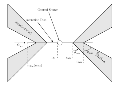
Our kinematic prescription for a biconical disc wind model follows Shlosman & Vitello (1993), and is described further by LK02, H13 and M15. The purpose of this purely kinematic wind model is to provide a simple tool for exploring different outflow geometries. A schematic is shown in Fig. 1, with key aspects marked. The general biconical geometry is similar to that invoked by Murray et al. (1995) and Elvis (2000) to explain the phenomenonology of quasars and BALQSOs. However, we do not include the initial vertical component present in the Elvis (2000) model, which was invoked as a qualitative explanation for narrow absorption lines.
3.1 Photon Sources
We include two sources of r-packets in our model: An accretion disc and a central X-ray source. The accretion disc is assumed to be geometrically thin, but optically thick. Accordingly, we treat the disc as an ensemble of blackbodies with a Shakura & Sunyaev (1973) effective temperature profile. The emergent SED is then determined by the specified accretion rate () and central BH mass (). All photon sources in our model are opaque, meaning that r-packets that strike them are destroyed. The inner radius of the disc extends to the innermost stable circular orbit (ISCO) of the BH. We assume a Schwarzchild BH with an ISCO at , where is the gravitational radius. For a BH, this is equal to or .
The X-ray source is treated as an isotropic sphere at the ISCO, which emits -packets according to a power law in flux with index , of the form
| (3) |
The normalisation, of this power law is such that it produces the specified 2-10 keV luminosity, . Photons, or -packets, produced by the accretion disc and central X-ray source are reprocessed by the wind. This reprocessing is dealt with by enforcing strict radiative equilibrium (modulo adiabatic cooling; see section 2.3) via an indivisible energy packet constraint (see Lucy 2002, M15).
3.2 Kinematics and Geometry
In the SV93 model, a biconical disc wind rises from the accretion disc between launch radii and . The opening angles of the wind are set to and . The poloidal velocity along each individual streamline at a poloidal distance is then given by (e.g. Rybicki & Hummer 1978)
| (4) |
where is the velocity at the base of the streamline, is an exponent governing how quickly the wind accelerations and is the ‘acceleration length’, defined as the distance at which the outflow reaches half of its terminal velocity, . The terminal velocity is set to a fixed multiple of the escape velocity, , at the base of the streamline (radius ). The rotational velocity, , is initially Keplerian (), and the wind conserves specific angular momentum, such that
| (5) |
The velocity law is crucial in determining the output spectra, as it affects not only the projected velocities along the line of sight, but also the density and ionization state of the outflow. A wind that accelerates more slowly will have a denser wind base with correspondingly different ionization and emission characteristics.
3.3 A Simple Approximation for Clumping
In our previous modelling efforts, we assumed a smooth outflow, in which the density at a given point was determined only by the kinematic parameters and mass loss rate. However, as already discussed, AGN winds exhibit significant substructure – the outflow is expected to be clumpy, rather than smooth, and probably on a variety of scales. A clumpy outflow offers a possible solution to the so-called ‘over-ionization problem’ in quasar and AGN outflows (e.g. Junkkarinen et al. 1983; Weymann et al. 1985; Hamann et al. 2013). This is the main motivation for incorporating clumping into our model.
Deciding on how to implement clumping into our existing wind models was not straightforward. First, and most importantly, the physical scale lengths and density contrasts in AGN outflows are not well-constrained from observations or theory. As a result, while one could envision in principle, clouds with a variety of sizes and density contrasts varying perhaps as function of radius, there would have been very little guidance on how to set nominal values of the various parameters of such a model. Second, there are significant computational difficulties associated with adequately resolving and realistically modelling a series of small scale, high density regions with a MCRT – or for that matter, a hydrodynamical – code. Given the lack of knowledge about the actual type of clumping, we have adopted a simple approximation used successfully in stellar wind modelling, known as microclumping (e.g. Hamann & Koesterke 1998; Hillier & Miller 1999; Hamann et al. 2008).
The underlying assumption of microclumping is that clump sizes are much smaller than the typical photon mean free path, and thus the clumps are both geometrically and optically thin. This approach allows one to treat clumps only in terms of their volume filling factor, , instead of having to specify separately their size and density distributions. In our model, is independent of position (see section 4.4). The inter-clump medium is modeled as a vacuum, although the outflow is still non-porous and axisymmetric. This approach therefore assumes that the inter-clump medium is unimportant in determing the output spectrum, which we expect to be true only when density constrasts are large and the inter-clump medium is both very ionized and of low emissivity and opacity. The density of the clumps is multiplied by the “density enhancement” . Opacities, , and emissivities, , can then be expressed as
| (6) |
Here the subscript denotes that the quantity is calculated using the enhanced density in the clump. The resultant effect is that, for fixed temperature, processes that are linear in density, such as electron scattering, are unchanged, as and will cancel out. However, any quantity that scales with the square of density, such as collisional excitation or recombination, will increase by a factor of . In our models, the temperature is not fixed, and is instead set by balancing heating and cooling in a given cell. In the presence of an X-ray source, this thermal balance is generally dominated by bound-free heating and line cooling. The main effect of including clumping in our modelling is that it moderates the ionization state due to the increased density. This allows an increase in the ionizing luminosity, amplifying the amount of bound-free heating and also increasing the competing line cooling term (thermal line emission).
The shortest length scale in a Sobolev MCRT treatment such as ours is normally the Sobolev length, given by
| (7) |
This is typically cm near the disc plane, increasing outwards. We use the mean density to calculate the Sobolev optical depth, which assumes that is greater than the typical clump size. Thus for the microclumping assumption to be formally correct, clumps should be no larger than cm. This size scale is not unreasonable for quasar outflows, as de Kool & Begelman (1995) suggest that BAL flows may have low filling factors with clump sizes of cm.
Our clumping treatment is necessarily simple; it does not adequately represent the complex substructures and stratifications in ionization state we expect in AGN outflows. Nevertheless, this parameterization allows simple estimates of the effect clumping has on the ionization state and emergent line emission.
3.4 The Simulation Grid
Using this prescription, we conducted a limited parameter search over a 5-dimensional parameter space involving the variables , , , and . The grid points are shown in Table 1. The aim here was to first fix and to their H13 values, and increase to erg s-1 (a more realistic value for a quasar of and an Eddington fraction of ; see section 4.3).
We then evaluated these models based on how closely their synthetic spectra reproduced the following properties of quasars and BALQSOs:
-
•
UV absorption lines with at of viewing angles (e.g. Knigge et al. 2010);
-
•
Line emission emerging at low inclinations, with Å in C iv Å (e.g. Shen et al. 2011);
-
•
H recombination lines with Å in Ly (e.g. Shen et al. 2011);
-
•
Mg ii and Al iii (LoBAL) absorption features with at a subset of BAL viewing angles;
-
•
Verisimilitude with quasar composite spectra.
Here is the ‘Balnicity Index’ (Weymann et al. 1991), given by
| (8) |
The constant everywhere, unless the normalized flux has satisfied continuously for at least km s−1, whereby is set to .
In the next section, we present one of the most promising models, which we refer to as the fiducial model, and discuss the various successes and failures with respect to the above criteria. This allows us to gain insight into fundamental geometrical and physical constraints and assess the potential for unification. We then discuss the sensitivity to key parameters in section 4.5. The full grid, including output synthetic spectra and plots can be found at jhmatthews.github.io/quasar-wind-grid/.
| Parameter | Grid Point Values | |||
|---|---|---|---|---|
| cm | cm | |||
4 Results and Discussion From A Fiducial Model
Here we describe the results from a fiducial model, and discuss these results in the context of the criteria presented in section 3.4. The parameters of this model are shown in Table 2. Parameters differing from the benchmark model of H13 are highlighted with an asterisk. In this section, we examine the physical conditions of the flow, and present the synthetic spectra, before comparing the X-ray properties of this particular model to samples of quasars and luminous AGN.
| Fiducial Model Parameters | Value |
|---|---|
| ∗ | |
| cm∗ | |
4.1 Physical Conditions and Ionization State
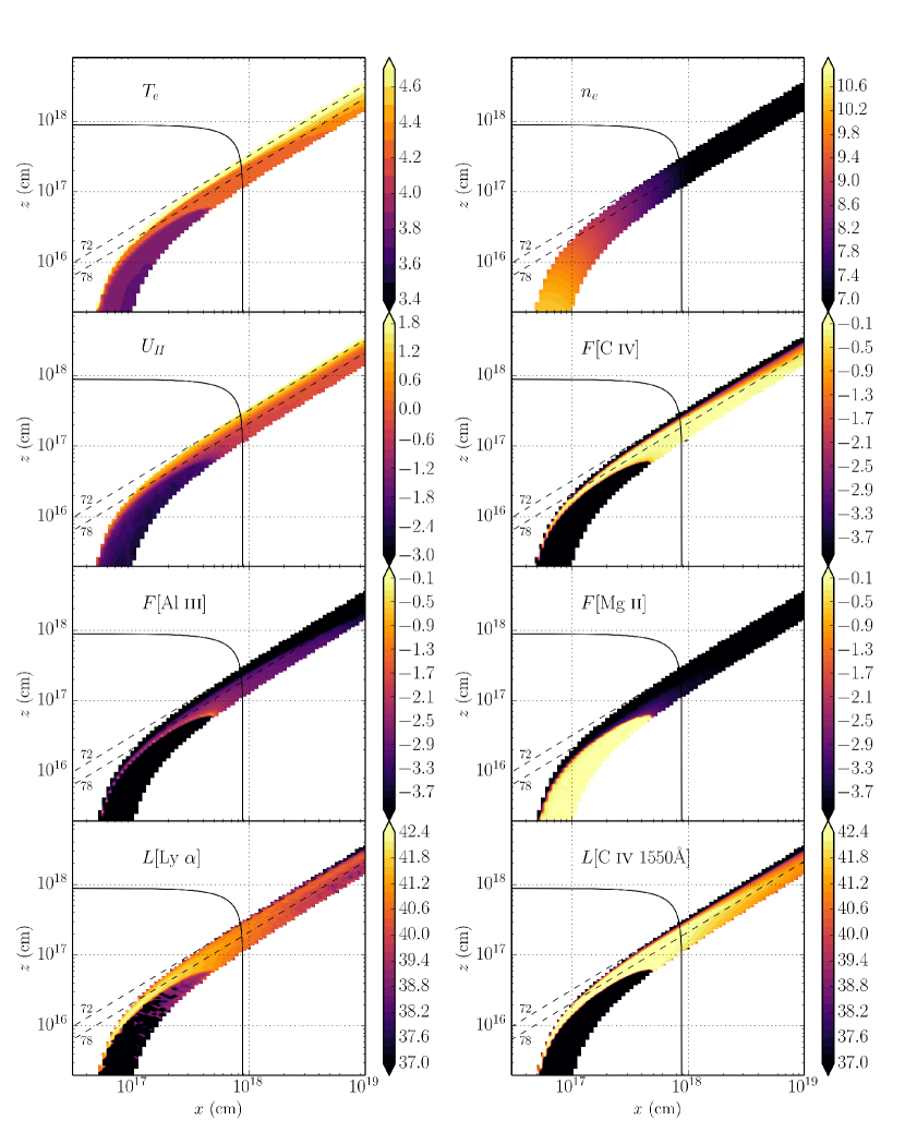
Fig. 2 shows the physical properties of the wind. The wind rises slowly from the disc at first, with densities within clumps of close to the disc plane, where is the local number density of H. The flow then accelerates over a scale length of up to a terminal velocity equal to the escape velocity at the streamline base (). This gradual acceleration results in a wind that exhibits a stratified ionization structure, with low ionization material in the base of the wind giving way to highly ionized plasma further out. This is illustrated in Fig. 2 by the panels showing the ion fraction of some important ions. With a clumped wind, we are able to produce the range of ionization states observed in quasars and BALQSOs, while adopting a realistic keV X-ray luminosity of . Without clumping, this wind would be over-ionized to the extent that opacities in e.g., C iv would be entirely negligible (see H13).
One common way to quantify the ionization state of a plasma is through the ionization parameter, , given by
| (9) |
where denotes photon frequency. Shown in Fig. 2, the ionization parameter is a useful measure of the global ionization state, as it represents the ratio of the number density of H ionizing photons to the local H density. It is, however, a poor representation of the ionization state of species such as C iv as it encodes no information about the shape of the SED. In our case, the X-ray photons are dominant in the photoionization of the UV resonance line ions. This explains why a factor of 100 increase in X-ray luminosity requires a clumping factor of 0.01, even though the value of decreases by only a factor of compared to H13.
The total line luminosity also increases dramatically compared to the unclumped model described by H13. This is because the denser outflow can absorb the increased X-ray luminosity without becoming over-ionized, leading to a hot plasma which produces strong collisionally excited line emission. This line emission typically emerges on the edge of the wind nearest the central source. The location of the line emitting regions is dependent on the ionization state, as well as the incident X-rays. The radii of these emitting regions is important, and can be compared to observations. The line luminosities, , shown in the figure correspond to the luminosity in of photons escaping the Sobolev region for each line. As shown in Fig. 2, the C iv Å line in the fiducial model is typically formed between (). This is in rough agreement with the reverberation mapping results of Kaspi (2000) for the quasar S5 0836+71, and also compares favourably with microlensing measurements of the size of the C iv Å emission line region in the BALQSO H1413+117 (O’Dowd et al. 2015).
4.2 Synthetic Spectra: Comparison to Observations
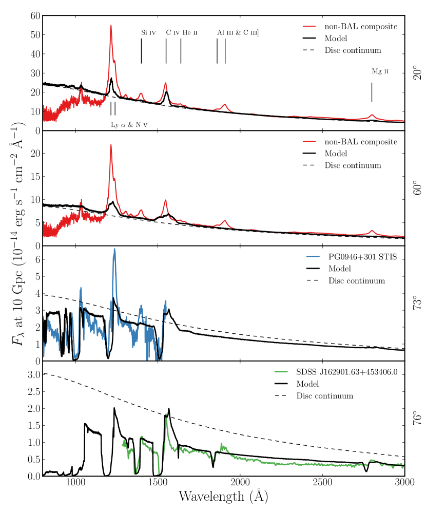
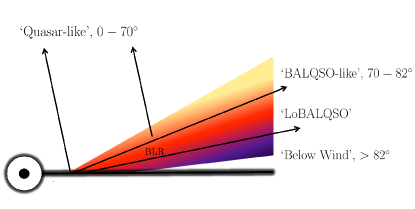
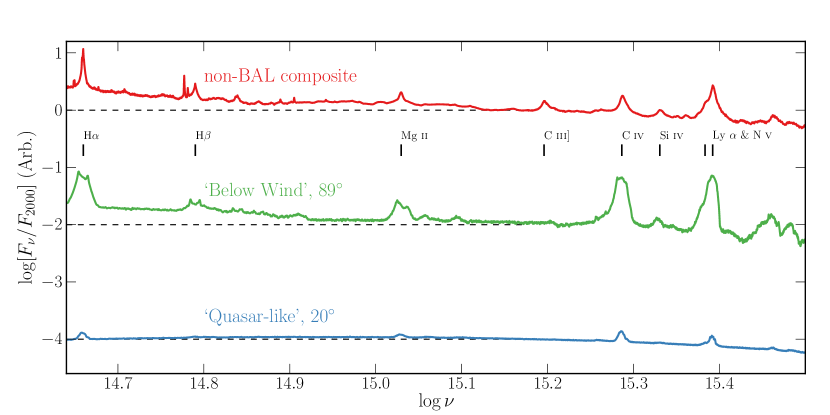
Fig. 3 shows the synthetic spectrum in the UV from the fiducial model. To assess the ability of the synthetic spectra to match real quasar spectra, we also show Sloan Digital Sky Survey (SDSS) quasar composites from Reichard et al. (2003), normalised to the flux at 2000Å for low inclinations. Unfortunately, the wide variety of line profile shapes and internal trough structure in BALQSOs tends to ‘wash out’ BAL troughs in composite spectra to the extent that BALQSO composites do not resemble typical BALQSOs. Because of this, we instead compare to a Hubble Space Telescope STIS spectrum of the high BALnicity BALQSO PG0946+301 (Arav et al. 2000), and an SDSS spectrum of the LoBAL quasar SDSS J162901.63+453406.0, for the angles of and , respectively. We show a cartoon illustrating how geometric effects determine the output spectra in Fig. 4.
4.2.1 Broad absorption lines (‘BALQSO-like’ angles)
The UV spectrum is characterised by strong BAL profiles at high inclinations (). This highlights the first success of our model: clumping allows the correct ionization state to be maintained in the presence of strong X-rays, resulting in large resonance line opacities. At the highest inclinations, the cooler, low ionization material at the base of the wind starts to intersect the line of sight. This produces multiple absorption lines in species such as Mg ii, Al iii and Fe ii. The potential links to LoBALQSOs and FeLoBALQSOs are discussed in section 2.4.
The high ionization BAL profiles are often saturated, and the location in velocity space of the strongest absorption in the profile varies with inclination. At the lowest inclination BAL sight lines, the strongest absorption occurs at the red edge, whereas at higher inclinations (and for the strongest BALs) the trough has a sharp edge at the terminal velocity. This offers one potential explanation for the wide range of BALQSO absorption line shapes (see e.g. Trump et al. 2006; Knigge et al 2008, Filiz Ak et al. 2014).
The absorption profiles seen in BALQSOs are often non-black, but saturated, with flat bases to the absorption troughs (Arav et al. 1999a, b). This is usually explained either as partial covering of the continuum source or by scattered contributions to the BAL troughs, necessarily from an opacity source not co-spatial with the BAL forming region. The scattered light explanation is supported by spectropolarimetry results (Lamy & Hutsemékers 2000). Our spectra do not show non-black, saturated profiles. We find black, saturated troughs at angles , and the BALs are non-saturated at lower inclinations. The reasons for this are inherent in the construction of our model. First, the microclumping assumption does not allow for porosity in the wind, meaning that it does not naturally produce a partial covering absorber. To allow this, an alternative approach such as macroclumping would be required (e.g. Hamann et al. 2008; Šurlan et al. 2012). Second, our wind does not have a significant scattering contribution along sightlines which do not pass through the BAL region, meaning that any scattered component to the BAL troughs is absorbed by line opacity. This suggests that either the scattering cross-section of the wind must be increased (with higher mass loss rates or covering factors), or that an additional source of electron opacity is required, potentially in a polar direction above the disc. We note the scattering contribution from plasma in polar regions is significant in some ‘outflow-from-inflow’ simulations (Kurosawa & Proga 2009; Sim et al. 2012).
4.2.2 Broad emission lines (‘quasar-like’ angles)
| Property | Synthetic, | Observed (S11) |
|---|---|---|
| [C iv] | ||
| [Mg ii] | ||
Unlike H13, we now find significant collisionally excited line emission emerges at low inclinations in the synthetic spectra, particular in the C iv and N v lines. We also find a strong Ly line and weak He ii Å line as a result of our improved treatment of recombination using macro-atoms. In the context of unification, this is a promising result, and shows that a biconical wind can produce significant emission at ‘quasar-like’ angles. To demonstrate this further, we show line luminosities and monochromatic continuum luminosities from the synthetic spectra in Table 3. These are compared to mean values from a subsample of the SDSS DR7 quasar catalog (Shen et al. 2011) with BH mass and Eddington fraction estimates similar to the fiducial model values (see caption). The spectra do not contain the strong C iii] 1909Å line seen in the quasar composite spectra, but this is due to a limitation of our current treatment of C; semi-forbidden (intercombination) lines are not included in our modelling.
In Fig. 5, we show an spectrum with broader waveband coverage that includes the optical, showing that our synthetic spectra also exhibit H and H emission. In this panel, we include a low inclination and also a very high inclination spectrum, which looks underneath the wind cone. This model shows strong line emission with very similar widths and line ratios to the quasar composites, and the Balmer lines are double peaked, due to velocity projection effects. Such double-peaked lines are seen in so-called ‘disc emitter’ systems (e.g. Eracleous & Halpern 1994) but not the majority of AGN. The line equivalent widths (EWs) increase at high inclination due to a weakened continuum from wind attenuation, disc foreshortening and limb darkening. This effect also leads to a redder continuum slope, as seen in quasars, which is due to Balmer continuum and Balmer and Fe ii line emission.
The viewing angle cannot represent a typical quasar within a unified model, as extreme inclinations should be extremely underrepresented in quasar samples. This is in part due to the compton-thick absorber or ‘torus’ expected at high inclinations (e.g. Antonucci & Miller 1985; Martínez-Sansigre et al. 2007). However, this spectrum does show that a wind model can naturally reproduce quasar emission lines if the emissivity of the wind is increased with respect to the disc continuum. In addition, it neatly demonstrates how a stratified outflow can naturally reproduce the range of ionization states seen in quasars.
Despite a number of successes, there are a some properties of the synthetic spectra that are at odds with the observations. First, the ratios of the EW of the Ly and Mg ii Å lines to the EW of C iv Å are much lower than in the composite spectra. Similar problems have also been seen in simpler photoionization models for the BLR (Netzer 1990). It may be that a larger region of very dense (cm-3) material is needed, which could correspond to a disc atmosphere or ‘transition region’ (see e.g. Murray et al. 1995; Knigge et al. 1997). While modest changes to geometry may permit this, the initial grid search did not find a parameter space in which the Ly or Mg ii EWs were significantly higher (see section 4.5). Second, we find that EWs increase with inclination (see Fig. 3 and Fig. 5; also Fig. 7), to the extent that, even though significantly denser models can match the line EWs fairly well at low inclinations, they will then possess overly strong red wings to the BAL P-Cygni profiles at high inclinations. The fact that the EW increase in our model are directly related to limb-darkening and foreshortening of the continuum. This appears to contradict observations, which show remarkably uniform emission line properties in quasars and BALQSOs (Weymann et al. 1991; DiPompeo et al. 2012). The angular distribution of the disc continuum and line emission is clearly crucially important in determining the emergent broad line EWs, as suggested by, e.g., the analysis of Risaliti et al. (2011). We shall explore this question further in a future study.
4.3 X-ray Properties
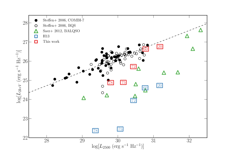
The main motivation for adding clumping to the model was to avoid over-ionization of the wind in the presence of strong X-rays. Having verified that strong BALs appear in the synthetic spectra, it is also important to assess whether the X-ray properties of this fiducial model agree well with quasar and BALQSO samples for the relevant inclinations.
Fig. 6 shows the emergent monochromatic luminosity () at 2 keV and plotted against at Å for a number of different viewing angles in our model. The monochromatic luminosities are calculated from the synthetic spectra and thus include the effects of wind reprocessing and attenuation. In addition to model outputs, we also show the BALQSO sample of Saez et al. (2012) and luminous AGN and quasar samples from Steffen et al. (2006). The best fit relation from Steffen et al. (2006) is also shown. For low inclination, ‘quasar-like’ viewing angles, we now find excellent agreement with AGN samples. The slight gradient from to in our models is caused by a combination of disc foreshortening and limb-darkening (resulting in a lower for higher inclinations), and the fact that the disk is opaque, and thus the X-ray source subtends a smaller solid angle at high inclinations (resulting in a lower for higher inclinations).
The high inclination, ‘BALQSO-like’ viewing angles show moderate agreement with the data, and are X-ray weak due to bound-free absorption and electron scattering in the wind. Typically, BALQSOs show strong X-ray absorption with columns of (Green & Mathur 1996; Mathur et al. 2000; Green et al. 2001; Grupe et al. 2003). This is often cited as evidence that the BAL outflow is shielded from the X-ray source, especially as sources with strong X-ray absorption tend to exhibit deep BAL troughs and high outflow velocities (Brandt et al. 2000; Laor & Brandt 2002; Gallagher et al. 2006). Our results imply that the clumpy BAL outflow itself can be responsible for the strong X-ray absorption, and supports Hamann et al.’s (2013) suggestion that geometric effects explain the weaker X-ray absorption in mini-BALs compared to BALQSOs.
4.4 LoBALs and Ionization Stratification
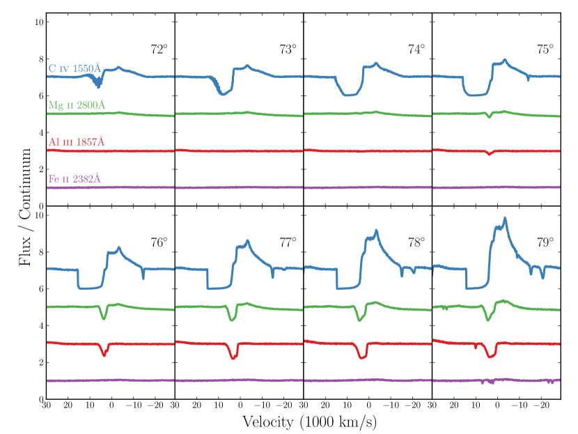
At high inclinations, the synthetic spectra exhibit blue-shifted BALs in Al iii and Mg ii– the absorption lines seen in LoBALQSOs, and we even see absorption in Fe ii at the highest inclinations. Line profiles in velocity space for C iv, Al iii and Mg ii, are shown in Fig. 7 for a range of BALQSO viewing angles. We find that ionization stratification of the wind causes lower ionization material to have a smaller covering factor, as demonstrated by figures 2 and 7. This confirms the behaviour expected from a unification model such as Elvis (2000). LoBALs are only present at viewing angles close to edge-on (), as predicted by polarisation results (Brotherton et al. 1997). As observed in a BALQSO sample by Filiz Ak et al. (2014), we find that BAL troughs are wider and deeper when low ionization absorption features are present, and high ionization lines have higher blue-edge velocities than the low ionization species.
There is also a correlation between the strength of LoBAL features and the amount of continuum attenuation at that sightline, particularly blueward of the Lyman edge as the low ionization base intersects the line-of-sight. A model such as this therefore predicts that LoBALQSOs and FeLoBALQSOs have stronger Lyman edge absorption and are more Compton-thick than HiBALQSOs and Type 1 quasars. An edge-on scenario also offers a potential explanation for the rarity of LoBAL and FeLoBAL quasars, due to a foreshortened and attenuated continuum, although BAL fraction inferences are fraught with complex selection effects (Goodrich 1997; Krolik & Voit 1998).
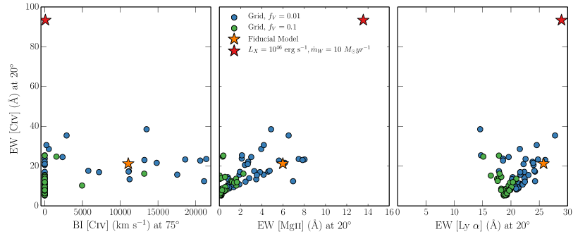
4.5 Parameter Sensitivity
Having selected an individual fiducial model from the simulation grid, it is important to briefly explore how specialised this model is, and how small parameter changes can affect the synthetic spectra. Fig. 8 shows the EW for C iv Å and Mg ii Å at a low inclination, and for C iv Å at a high inclination for the simulation grid. We find that almost all the models with are over-ionized, and fail to produce strong C iv BALs or emission lines. However, the models with generally produce C iv BALs and emission lines. The fiducial model is representative of this family of models and the spectra are generally similar, although it is clear from the figure that we have selected a model near the upper end of the EW distributions.
We find that it is difficult to significantly increase line emission while keeping the luminosity and mass loss rate of the system fixed. We show an additional point on figure 7 corresponding to a model with an order of magnitude higher X-ray luminosity and double the mass loss rate. As expected, this results in far higher line EWs, but fails to produce BALs because the collisionally excited emission swamps the BAL profile. In addition, this model would lie well above the expected relation in figure 5. Such a high X-ray luminosity could therefore not be the cause of the strong line emission seen in all Type 1 quasars.
The parameter search presented here is by no means exhaustive, and we may be limited by the specific parameterisation of the outflow kinematics we have used. Nevertheless, we suggest that the angular distribution of both the line and continuum emission is perhaps the crucial aspect to understand. With this in mind, obtaining reliable orientation indicators appears to be a crucial observational task if we are to further our understanding of BAL outflows and their connection, or lack thereof, to the broad line region.
5 Summary And Conclusions
We have carried out MCRT simulations using a simple prescription for a biconical disc wind, with the aim of expanding on the work of H13. To do this, we introduced two main improvements: First, we included a simple treatment of clumping, and second, we improved the modelling of recombination lines by treating H and He as ‘macro-atoms’. Having selected a fiducial model from an initial simulation grid, we assessed the viability of such a model for geometric unification of quasars, and found the following main points:
-
1.
Clumping the wind with a volume filling factor of moderates the ionization state sufficiently to allow for the formation of strong UV BALs while agreeing well with the X-ray properties of luminous AGN and quasars.
-
2.
A clumpy outflow model naturally reproduces the range of ionization states expected in quasars, due to its stratified density and temperature structure. LoBAL line profiles are seen at a subset of viewing angles, and Fe ii absorption is seen at particularly high inclinations.
-
3.
The synthetic spectra show a Ly line and weak He ii Å line as a result of our improved treatment of recombination using macro-atoms. We also see Balmer emission lines and a Balmer recombination continuum in the optical spectrum, but this is only really significant at high inclination where the continuum is suppressed.
-
4.
The higher X-ray luminosity causes a significant increase in the strength of the collisionally excited emission lines produced by the model. However, the equivalent-width ratios of the emission lines do not match observations, suggesting that a greater volume of dense ( cm-3) material may be required.
-
5.
The line EWs in the synthetic spectra increase with inclination. BAL and non-BAL quasar composites have comparable EWs, so our model fails to reproduce this behaviour. If the BLR emits fairly isotropically then for a foreshortened, limb-darkened accretion disc it is not possible to achieve line ratios at low inclinations that are comparable to those at high inclinations. We suggest that understanding the angular distribution of line and continuum emission is a crucial question for theoretical models.
Our work confirms a number of expected outcomes from a geometric unification model, and suggests that a simple biconical geometry such as this can come close to explaining much of the phenomenology of quasars. However, our conclusions pose some challenges to a picture in which BALQSOs are explained by an equatorial wind rising from a classical thin disc, and suggest the angular distribution of emission is important to understand if this geometry is to be refuted or confirmed. We suggest that obtaining reliable observational orientation indicators and exploring a wider parameter space of outflow geometries in simulations are obvious avenues for future work.
Acknowledgements
The work of JHM, SWM, NSH and CK is supported by the Science and Technology Facilities Council (STFC), via two studentships and a consolidated grant, respectively. CK also acknowledges a Leverhulme fellowship. We would like to thank the anonymous referee for a helpful and constructive report. We would like to thank Omer Blaes, Ivan Hubeny and Shane Davis for their assistance with Agnspec. We are grateful to Mike Brotherton, Mike DiPompeo, Sebastien Hoenig and Frederic Marin for helpful correspondence regarding polarisation measurements and orientation indicators. We would also like to thank Daniel Proga, Daniel Capellupo, Sam Connolly and Dirk Grupe for useful discussions. Simulations were conducted using Python version 80, and made use of the IRIDIS High Performance Computing Facility at the University of Southampton. Figures were produced using the matplotlib plotting library (Hunter 2007). This work made use of the Sloan Digital Sky Survey. Funding for the Sloan Digital Sky Survey has been provided by the Alfred P. Sloan Foundation, the U.S. Department of Energy Office of Science, and the Participating Institutions.
References
- Allen et al. (2011) Allen J. T., Hewett P. C., Maddox N., Richards G. T., Belokurov V., 2011, MNRAS 410, 860
- Antonucci & Miller (1985) Antonucci R. R. J., Miller J. S., 1985, ApJ 297, 621
- Arav et al. (1999a) Arav N., Becker R. H., Laurent-Muehleisen S. A., Gregg M. D., White R. L., Brotherton M. S., de Kool M., 1999a, ApJ 524, 566
- Arav et al. (1999b) Arav N., Korista K. T., de Kool M., Junkkarinen V. T., Begelman M. C., 1999b, ApJ 516, 27
- Badnell (2006) Badnell N. R., 2006, ApJs 167, 334
- Begelman et al. (1991) Begelman M., de Kool M., Sikora M., 1991, ApJ 382, 416
- Blandford & Payne (1982) Blandford R. D., Payne D. G., 1982, MNRAS 199, 883
- Brandt et al. (2000) Brandt W. N., Laor A., Wills B. J., 2000, ApJ 528, 637
- Brotherton et al. (1997) Brotherton M. S., Tran H. D., van Breugel W., Dey A., Antonucci R., 1997, ApJ Letters 487, L113
- Capellupo et al. (2014) Capellupo D. M., Hamann F., Barlow T. A., 2014, MNRAS 444, 1893
- Capellupo et al. (2011) Capellupo D. M., Hamann F., Shields J. C., Rodríguez Hidalgo P., Barlow T. A., 2011, MNRAS 413, 908
- Capellupo et al. (2012) Capellupo D. M., Hamann F., Shields J. C., Rodríguez Hidalgo P., Barlow T. A., 2012, MNRAS 422, 3249
- Carlberg (1980) Carlberg R. G., 1980, ApJ 241, 1131
- Cassidy & Raine (1996) Cassidy I., Raine D. J., 1996, A&A 310, 49
- Cohen et al. (1995) Cohen M. H., Ogle P. M., Tran H. D., Vermeulen R. C., Miller J. S., Goodrich R. W., Martel A. R., 1995, ApJ Letters 448, L77
- Cunto et al. (1993) Cunto W., Mendoza C., Ochsenbein F., Zeippen C. J., 1993, A&A 275, L5
- de Kool & Begelman (1995) de Kool M., Begelman M. C., 1995, ApJ 455, 448
- Dere et al. (1997) Dere K. P., Landi E., Mason H. E., Monsignori Fossi B. C., Young P. R., 1997, A&As 125, 149
- DiPompeo et al. (2012) DiPompeo M. A., Brotherton M. S., Cales S. L., Runnoe J. C., 2012, MNRAS 427, 1135
- Elvis (2000) Elvis M., 2000, ApJ 545, 63
- Emmering et al. (1992) Emmering R. T., Blandford R. D., Shlosman I., 1992, ApJ 385, 460
- Eracleous & Halpern (1994) Eracleous M., Halpern J. P., 1994, ApJs 90, 1
- Fabian (2012) Fabian A. C., 2012, ARAA 50, 455
- Filiz Ak et al. (2014) Filiz Ak N., Brandt W. N., Hall P. B., Schneider D. P., Trump J. R., Anderson S. F., Hamann F., Myers A. D., Pâris I., Petitjean P., Ross N. P., Shen Y., York D., 2014, ApJ 791, 88
- Fullerton (2011) Fullerton A. W., 2011, in C. Neiner, G. Wade, G. Meynet, G. Peters (eds.), IAU Symposium, Vol. 272, p. 136
- Gallagher et al. (2006) Gallagher S. C., Brandt W. N., Chartas G., Priddey R., Garmire G. P., Sambruna R. M., 2006, ApJ 644, 709
- Ganguly & Brotherton (2008) Ganguly R., Brotherton M. S., 2008, ApJ 672, 102
- Ganguly et al. (2006) Ganguly R., Sembach K. R., Tripp T. M., Savage B. D., Wakker B. P., 2006, ApJ 645, 868
- Ghosh & Punsly (2007) Ghosh K. K., Punsly B., 2007, ApJ Letters 661, L139
- Goodrich (1997) Goodrich R. W., 1997, ApJ 474, 606
- Goodrich & Miller (1995) Goodrich R. W., Miller J. S., 1995, ApJ Letters 448, L73
- Green et al. (2001) Green P. J., Aldcroft T. L., Mathur S., Wilkes B. J., Elvis M., 2001, ApJ 558, 109
- Green & Mathur (1996) Green P. J., Mathur S., 1996, ApJ 462, 637
- Grupe et al. (2003) Grupe D., Mathur S., Elvis M., 2003, AJ 126, 1159
- Hamann et al. (2013) Hamann F., Chartas G., McGraw S., Rodriguez Hidalgo P., Shields J., Capellupo D., Charlton J., Eracleous M., 2013, MNRAS 435, 133
- Hamann & Koesterke (1998) Hamann W.-R., Koesterke L., 1998, A&A 335, 1003
- Hamann et al. (2008) Hamann W.-R., Oskinova L. M., Feldmeier A., 2008, in W.-R. Hamann, A. Feldmeier, L. M. Oskinova (eds.), Clumping in Hot-Star Winds, 75
- Häring & Rix (2004) Häring N., Rix H.-W., 2004, ApJ Letters 604, L89
- Hazard et al. (1963) Hazard C., Mackey M. B., Shimmins A. J., 1963, Nature 197, 1037
- Higginbottom et al. (2013) Higginbottom N., Knigge C., Long K. S., Sim S. A., Matthews J. H., 2013, MNRAS 436, 1390
- Higginbottom et al. (2014) Higginbottom N., Proga D., Knigge C., Long K. S., Matthews J. H., Sim S. A., 2014, ApJ 789, 19
- Hillier (1991) Hillier D. J., 1991, A&A 247, 455
- Hillier & Miller (1999) Hillier D. J., Miller D. L., 1999, ApJ 519, 354
- Hunter (2007) Hunter J. D., 2007, Computing In Science & Engineering 9(3), 90
- Junkkarinen et al. (1983) Junkkarinen V. T., Burbidge E. M., Smith H. E., 1983, ApJ 265, 51
- Kellermann et al. (1989) Kellermann K. I., Sramek R., Schmidt M., Shaffer D. B., Green R., 1989, AJ 98, 1195
- King (2003) King A., 2003, ApJ Letters 596, L27
- King (2005) King A., 2005, ApJ Letters 635, L121
- Knigge et al. (1998) Knigge C., Long K. S., Wade R. A., Baptista R., Horne K., Hubeny I., Rutten R. G. M., 1998, ApJ 499, 414
- Knigge et al. (2008) Knigge C., Scaringi S., Goad M. R., Cottis C. E., 2008, MNRAS 386, 1426
- Krolik et al. (1981) Krolik J. H., McKee C. F., Tarter C. B., 1981, ApJ 249, 422
- Krolik & Voit (1998) Krolik J. H., Voit G. M., 1998, ApJ Letters 497, L5
- Kurosawa & Proga (2009) Kurosawa R., Proga D., 2009, ApJ 693, 1929
- Lamy & Hutsemékers (2000) Lamy H., Hutsemékers D., 2000, A&A 356, L9
- Landi et al. (2012) Landi E., Del Zanna G., Young P. R., Dere K. P., Mason H. E., 2012, ApJ 744, 99
- Laor & Brandt (2002) Laor A., Brandt W. N., 2002, ApJ 569, 641
- Long & Knigge (2002) Long K. S., Knigge C., 2002, ApJ 579, 725
- Lucy (2002) Lucy L. B., 2002, A&A 384, 725
- Lucy (2003) Lucy L. B., 2003, A&A 403, 261
- Lucy & Solomon (1970) Lucy L. B., Solomon P. M., 1970, ApJ 159, 879
- MacGregor et al. (1979) MacGregor K. B., Hartmann L., Raymond J. C., 1979, ApJ 231, 514
- Marscher (2006) Marscher A. P., 2006, in P. A. Hughes, J. N. Bregman (eds.), Relativistic Jets: The Common Physics of AGN, Microquasars, and Gamma-Ray Bursts, Vol. 856 of American Institute of Physics Conference Series, p. 1
- Martínez-Sansigre et al. (2007) Martínez-Sansigre A., Rawlings S., Bonfield D. G., Mateos S., Simpson C., Watson M., Almaini O., Foucaud S., Sekiguchi K., Ueda Y., 2007, MNRAS 379, L6
- Mathur et al. (2000) Mathur S., Green P. J., Arav N., Brotherton M., Crenshaw M., deKool M., Elvis M., Goodrich R. W., Hamann F., Hines D. C., Kashyap V., Korista K., Peterson B. M., Shields J. C., Shlosman I., van Breugel W., Voit M., 2000, ApJ Letters 533, L79
- Matthews et al. (2015) Matthews J. H., Knigge C., Long K. S., Sim S. A., Higginbottom N., 2015, MNRAS 450, 3331
- Murray et al. (1995) Murray N., Chiang J., Grossman S. A., Voit G. M., 1995, ApJ 451, 498
- Netzer (1990) Netzer H., 1990, in R. D. Blandford, H. Netzer, L. Woltjer, T. J.-L. Courvoisier, M. Mayor (eds.), Active Galactic Nuclei, p. 57
- Noebauer et al. (2010) Noebauer U. M., Long K. S., Sim S. A., Knigge C., 2010, ApJ 719, 1932
- O’Dowd et al. (2015) O’Dowd M. J., Bate N. F., Webster R. L., Labrie K., Rogers J., 2015, ArXiv e-prints
- Owocki & Rybicki (1984) Owocki S. P., Rybicki G. B., 1984, ApJ 284, 337
- Pelletier & Pudritz (1992) Pelletier G., Pudritz R. E., 1992, ApJ 394, 117
- Perley et al. (1984) Perley R. A., Dreher J. W., Cowan J. J., 1984, ApJ Letters 285, L35
- Potash & Wardle (1980) Potash R. I., Wardle J. F. C., 1980, ApJ 239, 42
- Pounds & Reeves (2009) Pounds K. A., Reeves J. N., 2009, MNRAS 397, 249
- Proga et al. (2014) Proga D., Jiang Y.-F., Davis S. W., Stone J. M., Smith D., 2014, ApJ 780, 51
- Proga & Kallman (2004) Proga D., Kallman T. R., 2004, ApJ 616, 688
- Proga & Kurosawa (2010) Proga D., Kurosawa R., 2010, in L. Maraschi, G. Ghisellini, R. Della Ceca, F. Tavecchio (eds.), Accretion and Ejection in AGN: a Global View, Vol. 427 of Astronomical Society of the Pacific Conference Series, 41
- Proga et al. (2000) Proga D., Stone J. M., Kallman T. R., 2000, ApJ 543, 686
- Reeves et al. (2003) Reeves J. N., O’Brien P. T., Ward M. J., 2003, ApJ Letters 593, L65
- Reichard et al. (2003) Reichard T. A., Richards G. T., Hall P. B., Schneider D. P., Vanden Berk D. E., Fan X., York D. G., Knapp G. R., Brinkmann J., 2003, AJ 126, 2594
- Risaliti et al. (2002) Risaliti G., Elvis M., Nicastro F., 2002, ApJ 571, 234
- Risaliti et al. (2011) Risaliti G., Salvati M., Marconi A., 2011, MNRAS 411, 2223
- Rybicki & Hummer (1978) Rybicki G. B., Hummer D. G., 1978, ApJ 219, 654
- Shakura & Sunyaev (1973) Shakura N. I., Sunyaev R. A., 1973, A&A 24, 337
- Shen et al. (2011) Shen Y., Richards G. T., Strauss M. A., Hall P. B., Schneider D. P., Snedden S., Bizyaev D., Brewington H., Malanushenko V., Malanushenko E., Oravetz D., Pan K., Simmons A., 2011, ApJs 194, 45
- Shlosman & Vitello (1993) Shlosman I., Vitello P., 1993, ApJ 409, 372
- Shlosman et al. (1985) Shlosman I., Vitello P. A., Shaviv G., 1985, ApJ 294, 96
- Silk & Rees (1998) Silk J., Rees M. J., 1998, A&A 331, L1
- Sim et al. (2005) Sim S. A., Drew J. E., Long K. S., 2005, MNRAS 363, 615
- Sim et al. (2008) Sim S. A., Long K. S., Miller L., Turner T. J., 2008, MNRAS 388, 611
- Sim et al. (2010) Sim S. A., Miller L., Long K. S., Turner T. J., Reeves J. N., 2010, MNRAS 404, 1369
- Sim et al. (2012) Sim S. A., Proga D., Kurosawa R., Long K. S., Miller L., Turner T. J., 2012, MNRAS 426, 2859
- Simon & Hamann (2010) Simon L. E., Hamann F., 2010, MNRAS 409, 269
- Sobolev (1957) Sobolev V. V., 1957, SvA 1, 678
- Sobolev (1960) Sobolev V. V., 1960, Moving envelopes of stars
- Springel et al. (2005) Springel V., Di Matteo T., Hernquist L., 2005, ApJ Letters 620, L79
- Sutherland (1998) Sutherland R. S., 1998, MNRAS 300, 321
- Tombesi et al. (2010) Tombesi F., Cappi M., Reeves J. N., Palumbo G. G. C., Yaqoob T., Braito V., Dadina M., 2010, A&A 521, A57
- Turner & Miller (2009) Turner T. J., Miller L., 2009, AAPR 17, 47
- Šurlan et al. (2012) Šurlan B., Hamann W.-R., Kubát J., Oskinova L. M., Feldmeier A., 2012, A&A 541, A37
- Verner et al. (1996) Verner D. A., Ferland G. J., Korista K. T., Yakovlev D. G., 1996, ApJ 465, 487
- Weymann et al. (1991) Weymann R. J., Morris S. L., Foltz C. B., Hewett P. C., 1991, ApJ 373, 23
- Weymann et al. (1982) Weymann R. J., Scott J. S., Schiano A. V. R., Christiansen W. A., 1982, ApJ 262, 497
- Weymann et al. (1985) Weymann R. J., Turnshek D. A., Christiansen W. A., 1985, in J. S. Miller (ed.), Astrophysics of Active Galaxies and Quasi-Stellar Objects, p. 333
- Zhou et al. (2006) Zhou H., Wang T., Wang H., Wang J., Yuan W., Lu Y., 2006, ApJ 639, 716