Laboratori Nazionali di Frascati, INFN, Frascati, Italy 33institutetext: CEA, Centre de Saclay, IRFU/Service de Physique Nucléaire, F-91191 Gif-sur-Yvette, France
GPD phenomenology and DVCS fitting
Abstract
We review the phenomenological framework for accessing Generalized Parton Distributions (GPDs) using measurements of Deeply Virtual Compton Scattering (DVCS) from a proton target. We describe various GPD models and fitting procedures, emphasizing specific challenges posed both by the internal structure and properties of the GPD functions and by their relation to observables. Bearing in mind forthcoming data of unprecedented accuracy, we give a set of recommendations to better define the pathway for a precise extraction of GPDs from experiment.
1 Introduction
1.1 The physics case
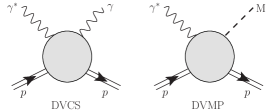
Generalized Parton Distributions (GPDs) were introduced in 1994 Mueller:1998fv and rediscovered independently in 1997 Radyushkin:1996nd ; Ji:1996nm . This branch of QCD studies grew rapidly because of their unique properties. GPDs are related to other nonperturbative objects that were studied independently beforehand: Parton Distribution Functions (PDFs) and Form Factors (FFs). In the infinite-momentum frame, PDFs describe the longitudinal momentum distributions of partons inside a hadron, and FFs are the Fourier transform of the hadron charge distribution in the transverse plane. GPDs naturally encompass PDFs and FFs in the case of all hadrons, and they also extend the notion of a Distribution Amplitude (DA) in the pion case. This generality is remarkably complemented by one outstanding feature: GPDs are directly related to the matrix element of the QCD energy-momentum tensor sandwiched between hadron states. This is both welcome and surprising because the energy-momentum tensor in canonically probed through gravity. GPDs bring the considered energy-moment̄um matrix element within experimental grasp through electromagnetic scattering. It was indeed realized early on that, owing to the factorization property of QCD, exclusive electroproduction of a real photon or a meson off a nucleon target at high momentum transfer is theoretically the cleanest way to access GPDs. The processes of Deeply Virtual Compton Scattering (DVCS), and Deeply Virtual Meson Production (DVMP) are shown in fig. 1. The access to GPDs through DVCS and DVMP is indirect because DVCS does not depend directly on GPDs, but on Compton Form Factors (CFFs), i.e. integrals of GPDs weighted by a specific kernel that is integrated order by order in perturbation theory.
Nevertheless, pioneering studies Airapetian:2001yk ; Adloff:2001cn ; Stepanyan:2001sm demonstrated the feasibility of DVCS measurements. They were followed by numerous dedicated experiments Chekanov:2003ya ; Aktas:2005ty ; Chen:2006na ; Airapetian:2006zr ; MunozCamacho:2006hx ; Mazouz:2007aa ; Aaron:2007ab ; Girod:2007aa ; Airapetian:2008aa ; Chekanov:2008vy ; Gavalian:2008aa ; Aaron:2009ac ; Airapetian:2009aa ; Airapetian:2010aa ; Airapetian:2010ab ; Airapetian:2011uq ; Airapetian:2012mq ; Pisano:2015iqa ; Jo:2015ema ; Defurne:2015kxq during a period of intense theoretical activity which put DVCS under solid control. In particular let us mention the full description of DVCS up to twist-3 Belitsky:2001ns ; Belitsky:2008bz ; Belitsky:2010jw ; Belitsky:2012ch , including the discussion of QED gauge invariance Anikin:2000em ; Radyushkin:2000ap ; Kivel:2000fg ; Belitsky:2000vx and target mass and finite momentum transfer corrections Braun:2012bg ; Braun:2012hq , the computation of higher orders in the perturbative expansion in the strong running coupling Ji:1997nk ; Belitsky:1997rh ; Mankiewicz:1997bk ; Ji:1998xh ; Belitsky:1999sg ; Freund:2001hm ; Freund:2001rk ; Freund:2001hd ; Pire:2011st ; Moutarde:2013qs , and the soft-collinear resummation of DVCS Altinoluk:2012fb ; Altinoluk:2012nt . Two closely related processes, Timelike Compton Scattering (TCS) Berger:2001xd ; Boer:2015hma and Double Deeply Virtual Compton Scattering (DDVCS) Guidal:2002kt ; Belitsky:2002tf ; Belitsky:2003fj have also been discussed, and receive now considerable attention from the experimental community.
Fits to DVCS data have been successfully performed since 2008 Kumericki:2007sa ; Guidal:2008ie ; Kumericki:2009uq ; Moutarde:2009fg ; Guidal:2009aa ; Guidal:2010ig ; Guidal:2010de ; Goldstein:2010gu ; Kumericki:2011zc ; Kumericki:2011rz ; GonzalezHernandez:2012jv ; Kumericki:2013br ; Boer:2014kya , providing first quantitative experimental information on CFFs. Although these fits do not give a final word on the GPD studies, they nevertheless show that the field is in a good shape from both theoretical and experimental perspectives. The new era about to start will yield data of unprecedented accuracy and with a wide kinematic coverage. The valence region is being explored again in Jefferson Lab (JLab) with the beginning of the experiments at 12 . The COMPASS Collaboration at CERN will soon start DVCS data-taking. GPDs and their golden channel DVCS, are at the heart of the physics case of a planned future Electron-Ion Collider (EIC).
The continuous progress in the field of GPDs has been documented in several review articles Ji:1998pc ; Goeke:2001tz ; Diehl:2003ny ; Belitsky:2005qn ; Boffi:2007yc ; Guidal:2013rya ; Muller:2014sha . The present text aims at preparing the ground for fits of forthcoming experimental data. How can GPD fitters work best with high-precision data? The community of PDF fitters is older and larger than its GPD analogue, and it has achieved an impressive level of accuracy and sophistication. GPD phenomenology is much harder, owing to the fact, in particular, that GPDs depend on more variables and are subject to many constraints. Considering PDF fits as an inspiring guideline, it is nevertheless possible to see which steps should be made to achieve a similar level of rigour over a shorter period of time.
Our review consists of three parts. In the remainder of sec. 1 we list the various constraints on GPDs, e.g., coming from discrete symmetries or Lorentz invariance. We also review several representations that fulfil such constraints, and present selection of GPD models within each framework. The intricacy of GPD modelling is one of the distinctive features of the field. In sec. 2, we present both the theoretical and experimental state of the art of DVCS, including various fitting strategies and lessons obtained from fits. In the last part, sec. 3, we give an outlook on future directions in the field of GPD fitting, and we suggest a few avenues towards improving present fitting procedures. In particular, we stress the need for establishing code benchmarking criteria for the various parametrizations. These would include introducing a set of uniform conventions for observable definitions, notations and data descriptions, and a thorough analysis of both the experimental and theoretical uncertainties.
Finally, this review is mostly dedicated to discussing GPDs and their extraction from DVCS on a nucleon target. For other related processes, we refer the reader to the reviews in ref. Favart:2015epja (DVMP), ref. Dupre:2015epja (nuclear DVCS), and to ref. Amrath:2008vx (DVCS from a pion).
1.2 Notations
For any four-vector we define the light cone coordinates by:
| (1) |
denotes the scalar product of two four-vectors and . Indices between parentheses will mean symmetrization (and average) over indices, e.g. .
We will consider hadron matrix elements of the form for different operators sandwiched between incoming (1) and outgoing (2) states. The total momentum and momentum transfer are:
| (2) | |||||
| (3) |
In terms of Mandelstam variables: .
We will denote by the GPD variable known as skewness, see eq. (11) below, and keep the symbol for the kinematic variable approximately equal to , where is the usual Bjorken scaling variable. M will stand for the proton mass, and for the particle fractional electric charge in units of the positron charge . Furthermore, is the Heaviside step function, a Dirac matrix, , and is the metric tensor. More specifically, (resp. ) will denote the photon virtuality in the DVCS channel (resp. TCS channel).
We will follow the convention of Diehl Diehl:2003ny to define GPDs in impact parameter space. The transverse plane Fourier transform of a function thus writes
| (4) |
with
| (5) |
and
| (6) |
being the maximal for given .
To simplify equations, we often drop the explicit dependence on unused variables when no confusion is possible. We will simply mention LO, NLO, …for ”Leading Order”, ”Next-to-Leading Order”, …when referring to perturbative expansions in the strong running coupling constant.
1.3 GPD definition and properties
1.3.1 Definition
GPDs are defined in the unpolarized (vector) sector as
| (7) |
| (8) |
and in the polarized (axial-vector) sector as
| (9) |
| (10) |
where the skewness reads
| (11) |
and where we suppressed polarization dependence and Wilson lines in the bilocal operators (which serve to restore gauge invariance).
Both and can be decomposed as
| (12) | ||||
| (13) |
where the Dirac spinor bilinears are
| (14) | ||||||
| (15) |
and the spinors are normalized so that . The GPDs above are defined following Refs. Diehl:2003ny ; Belitsky:2005qn . See table 1 with equivalent symbols.
Four additional GPDs can be defined at twist two in the helicity flip (tensor) sector,
| (16) |
where . Notice that the operator defining these GPDs is chiral-odd, i.e., it flips quark chirality, as opposed to the chiral-even operators in eqs. (7-10). The chiral-odd quark GPDs cannot be measured directly in DVCS. They are accessible through exclusive pseudoscalar meson production Ahmad:2008hp ; Goloskokov:2009ia ; Goloskokov:2011rd . Analogously in the gluon sector
| (17) |
where and the symbol indicates symmetrization and trace subtraction of uncontracted indices.
For a complete classification of GPDs and of their parton correlation function substructure up to twist four see refs. Meissner:2008ay ; Meissner:2009ww ; Lorce:2013pza .
| this work | ref. Belitsky:2005qn | ref. Diehl:2003ny |
1.3.2 Forward limit
In the forward kinematic limit, , some GPDs reduce to standard PDFs,
| (18) | ||||
| (19) | ||||
| (20) | ||||
| (21) | ||||
| (22) |
1.3.3 Discrete symmetries
Time reversal and hermiticity imply that GPDs are real and that
| (23) |
for all . From now on, and unless explicitly specified, we will assume .
The fact that the gluon is its own antiparticle implies that
| (24) | ||||
| (25) |
For quarks it is useful to consider the combinations,
| (26) | ||||
| (27) |
with similar relations involving and . in forward limit reduces to so is called singlet (although it has to be summed over flavors to really become singlet), and is called non-singlet or valence combination.
If one considers -parity exchanged in the -channel corresponding to each GPD, then , and both gluon GPDs are -even, while and are -odd. In DVCS there is no change of going from initial to final state, so only -even GPDs contribute.
1.3.4 Sum rules
Sum rules are quite important in the GPD phenomenology. The integrals of GPDs over are related to the quark contributions and to the elastic form factors and in the Pauli-Dirac representation,
| (28) | ||||
| (29) |
with similar relations relating and to the axial and pseudoscalar form factors and . Sum rules can be seen as a particular case of the polynomiality property discussed in sec. 1.3.5, and the connection of GPDs to both PDFs and FFs provides a particularly interesting physical interpretation.
Ji’s sum rule Ji:1996ek is another landmark GPD property. The Belinfante energy-momentum tensor Belinfante:1939em ; Rosenfeld:1940em between nucleon states can be parametrized as,
| (30) |
where , and are called gravitational form factors, defined for both the quark and gluon sectors. The derivation of Ji’s sum rule starts from the decomposition of the nucleon spin into its quark and gluon contributions
| (31) |
with both terms related to the energy-momentum tensor
| (32) |
One can then connect the gravitational form factors with the coefficients of the correlation function defined using eqs.(7,12,15)
| (33) |
(an analogous decomposition can be made in the gluon sector). The second Mellin moments of the GPDs and from this definition are,
| (34) | |||||
| (35) |
so that
| (36) |
A closer look reveals that the contribution related to is already known from PDFs. In other words
| (37) |
The first term on the RHS is the quark total momentum which can be obtained from standard measurements of PDFs in Deeply Inelastic Scattering (DIS). The second term is the new component in the sum rule: since the quark spin contribution is already known, the second term relates to both the quark orbital motion and to the nucleon’s magnetic properties. Measuring the GPD became one of the main motivations of the experimental GPD program, including the physics case for an EIC Kumericki:2011zc ; Accardi:2012qut ; Aschenauer:2013hhw .
More recent developments have been addressing the question of a gauge invariant decomposition of total angular momentum into its spin and orbital components,
| (38) |
A decomposition of the quark angular momentum in Ji’s sum rule, namely,
| (39) |
can be performed, where the LHS is described by the GPDs and , eq. (36), while on the RHS, is described by a specific twist-three GPD Penttinen:2000dg ; Kiptily:2002nx ; Hatta:2012cs ; Courtoy:2013oaa , and is the total quark helicity. An analogous decomposition in the gluon sector is not possible in this case. We refer to the recent reviews Leader:2013jra ; Liu:2015xha for further details on these developments.
Finally, the angular momentum sum rule was extended to a spin-1 system, e.g. the deuteron in ref. Taneja:2011sy . The sum rule reads
| (40) |
where is one of the five deuteron GPDs in the vector sector Berger:2001zb . It is interesting to notice that, analogously to the nucleon case, the angular momentum is determined by the same GPD, whose first Mellin moment is the magnetic form factor of the spin-1 system.
1.3.5 Polynomiality
Related to sum-rules is the important polynomiality property of GPDs. Namely, using identities
| (41) |
| (42) |
and the behavior of GPDs under discrete symmetries (see sec. 1.3.3), one can show that moments of quark GPDs are even polynomials in with leading powers given in table 2 and that moments of gluon GPDs are polynomials in with leading powers given in table 3.
| GPD | even | odd |
|---|---|---|
| , | ||
| , |
| GPD | even | odd |
|---|---|---|
| , | 0 | |
| 0 | ||
| , | 0 |
Zeros in table 3 are due to the (anti)symmetry of gluon GPDs, see eqs. (24) and (25). Note that the zeroth () moment of quark GPD leads to -independence explicated by the sum rules (28) and (29). Also note that the first moment of combination is also -independent, as explicated in Ji’s sum rule (36).
1.3.6 Positivity
Positivity bounds emerge from the definition of the norm on a Hilbert space, and thus are fundamental properties of GPDs. For the sake of simplicity, we will discuss the case of spinless hadrons. In essence, positivity bounds are inequalities between GPDs and the corresponding PDFs at well-defined kinematic configurations Pire:1998nw ; Radyushkin:1998es ; Pobylitsa:2002iu , e.g.
| (43) |
where the naming convention of and
| (44) | |||||
| (45) |
will become evident in sec. 1.4.1. This is a strong model-independent constraint. Consider for example a pion PDF computed in the Bethe-Salpeter approach with a proper implementation of the symmetry typical of two-body problems Chang:2014lva . From perturbative QCD, we know that the PDF vanishes like when is close to 1. From the exchange symmetry , we observe that the PDF should vanish at the same pace when is close to 0. In particular, we conclude from eq. (43) that a GPD computed consistently in that framework should vanish on the crossover line . This is completely consistent with the result of ref. Ji:2006cr where all possible states were consistently introduced to obtain a pion GPD model with a nonzero value on the crossover line.
The derivation of an inequality such as eq. (43) proceeds from the Cauchy-Schwarz inequality. The matrix element defining a GPD can be identified as an inner product of two different states. Its absolute value is smaller than the product of the norms of these two states, and each of these two terms is recognized as the matrix element defining a PDF. This is basically the underlying reasoning of refs. Pobylitsa:2001nt ; Pobylitsa:2002gw and refs. therein. From this derivation, the positivity bounds are restricted to the DGLAP regions .
This argument can however be made more general: as a guideline, we may remember the proof of Cauchy-Schwarz inequality. Consider a real inner product , two vectors , in a real Hilbert space, and a real . From the positivity of for all , we derive . The positivity of the norm of the Hilbert space of quark-hadron states is at the heart of the argument. In ref. Pobylitsa:2002iu Pobylitsa derived inequalities from the positivity of the norm of arbitrary superpositions of states , where the sum runs over various hadron states of momentum and spin , with the (good component of the) quark field taken at point and weighted by arbitrary functions . This procedure yields infinitely many inequalities, all translating in various forms the positive definiteness of the norm. From the model-building point of view, this fact makes positivity bounds an even more severe constraint. All of these inequalities admit the following generic form in the impact parameter representation Pobylitsa:2002iu
| (46) |
for arbitrary function , and where represents the matrix element defining GPDs in impact parameter space. At last, representing explicitly a GPD as an inner product Pobylitsa:2002vi
| (47) |
where the sum can range over a discrete or continuous collection of functions, guarantees the fulfillment of eq. (46) (after the change of variables which maps such that to in .
For completeness, we mention that the stability of positivity bounds under LO evolution is established in ref. Pobylitsa:2002iu . The sign of the norm of (unphysical) quark-hadron states is questioned in ref. Pobylitsa:2002ru where an alternative proof of the positivity bounds is given.
1.4 GPD parametrizations
In the years following the introduction of GPDs and the definition of their fundamental physical properties, several frameworks have been defined that provide parametric forms to be used for their extraction from experimental data. This theoretical progress has been proceeding simultaneously to the development of various experimental programs to measure GPDs (see sec. 2.5). In what follows we give a list of the frameworks or representations that have been used for data interpretation, followed by a description of specific models within each framework.
1.4.1 Overlap
This representation bears its name from the description of a GPD as an overlap of light front wave functions. This representation was derived by Diehl et al. Diehl:2001xx . Here again we will only discuss the quark sector, the gluon sector following mutatis mutandis. We will mostly use the notations of ref. Diehl:2001xx , but will restrict ourselves to spinless hadrons for brevity.
A Fock state made of partons is generically denoted where encode the information about the partons: their type, their helicity and their color. A hadron state with momentum is made of an arbitrary number of partons, weighted by corresponding light front wave functions
| (48) |
where the symbols and are compact notations for
| (49) | |||||
| (50) |
The light front wave function normalization is derived from the hadron state covariant normalization, i.e. including contributions from all parton states
| (51) |
The next step consists in expanding the good component of the quark field in terms of operators creating Fock states with given plus and transverse momenta, helicity and color. The active parton is emitted from the hadron, and later absorbed by it, while the other partons are spectators. The wave functions depend on momentum components relative to the considered hadron momentum. This kinematic matching is made in frames where the incoming or outgoing hadron have zero transverse momentum, hence the terminology ”in” and ”out” for kinematic variables relevant to the DGLAP region
| (52) | |||||
| (53) |
The ”out” variables are simply obtained by changing to and to .
In this region the overlap representation of the GPD writes
| (54) |
The overlap representation has a similar structure in the other DGLAP region . Considering eq. (47), this is enough to ensure that every model built from the overlap representation will fulfil positivity bounds. Furthermore, the overlap representation can even be used as a first principle statement to establish a general form for the positivity bounds, e.g. as in ref. Diehl:2003ny .
However, the result in the ERBL region involves the overlap of wave functions with and constituents. The polynomiality property relates in this case wave functions with different partonic contents. This poses a constraint on the building of GPD models from the overlap representation. Recent progress in this direction will be discussed in sec. 1.4.3.
1.4.2 Covariant Scattering Matrix Approach
The backdrop for this approach is a gauge invariant extension at leading twist of the covariant parton model ref. Landshoff:1970ff ; Brodsky:1973hm . The structure functions/PDFs for DIS processes as well as the CFFs/GPDs in DVCS result directly from the analytic behavior of the quark/gluon-proton scattering amplitude. The parton-proton amplitude defined in this framework is a holomorphic function of the parton’s four-momentum component, .
An important aspect of the covariant scattering matrix approach is in its covariant regularization which can be carried out in different ways depending on the specific model. An even more interesting feature is that it provides a natural framework where Regge behavior of the structure functions can be naturally connected to their Bjorken scaling property Brodsky:1973hm . The models we consider here correspond to the lowest order in perturbation theory. At this order the scattering amplitude includes two vertices with a proton, a parton undergoing the hard scattering, and a spectator system. The latter corresponds to a scalar or an axial vector spectator/recoiling system, namely a diquark for the valence quark distribution, or a tetraquark or higher diquark excited states for the sea quarks. It is instead an octet three quarks system, for the gluon distribution.
The propagator structure of the covariant amplitude is given by,
| (55) | |||||
where are the Mandelstam invariants, and are the initial and final quark four-momentum squared, is quark mass, is the spectator system four-momentum squared, is its mass, and is a vertex function. As we will see in the model section can be taken as a pointlike coupling, in which case a regularization à la Pauli Villars applies, or as falling of with , thus providing a covariant ultraviolet cutoff.
The analytic behavior of is such that the spectator is placed on-shell while the struck parton is off-shell in the DGLAP region ( and ). Vice versa in the ERBL region it is the struck parton to be placed on-shell.
Taking into account the spin structure of the particles involved results in a more complicated structure in the numerator of eq. (55), without, however, changing its analytic behavior. In this case, the quark/gluon-proton scattering amplitude depends directly on the initial (final) parton helicity, and the initial (final) proton helicity, , namely,
The condition of polynomiality in this approach is satisfied automatically, due to the covariance of the amplitude. In practical models which rely on approximations, this property has to nevertheless be tested.
The advantage of the covariant scattering matrix approach is in that it allows one to describe Regge behavior of the GPDs at low . This is accomplished by allowing for a spectral distribution for the spectator mass characterized by a peak at low mass values GeV, and a behavior , at GeV (where is the Regge intercept parameter). As we show in sec. 1.5.3, the dependence can also be described in this scenario.
1.4.3 Double Distributions
Double Distributions (DDs) were introduced first by Müller et al. under the name spectral functions Mueller:1998fv and later rediscovered by Radyushkin Radyushkin:1998es ; Radyushkin:1998bz . They offer the attractive feature of naturally solving the polynomiality constraint exposed in sec. 1.3.5. We will explain below why it is so by considering the quark sector, but the extension to the gluon sector is straightforward.
The quark DDs and of a spinless hadron are defined by the following matrix element Polyakov:1999gs :
| (56) |
They are related to the GPD through:
| (57) |
The physical domain of GPDs (with ) restricts the support of the DDs to the rhombus . As emphasized by Teryaev Teryaev:2001qm and Tiburzi Tiburzi:2004qr , there are infinitely many parameterizations for DDs yielding the same GPDs. Consider for example an arbitrary function vanishing111We refer to ref. Tiburzi:2004qr for a detailed discussion of boundary conditions on . on the boundary of the rhombus . The transformation:
| (58) | |||||
| (59) |
leaves the GPD in eq. (57) unchanged. In particular, there is one particular transformation Belitsky:2000vk allowing the description of the two DDs and in terms of one single function :
| (60) | |||||
| (61) |
This choice is referred to as One-Component Double Distribution (1CDD) in ref. Belitsky:2005qn and was recently used for model building and theoretical considerations Radyushkin:2011dh ; Radyushkin:2012gba ; Radyushkin:2013hca ; Radyushkin:2013bba ; Mezrag:2013mya . The relation (57) between the GPD and the 1CDD now is:
| (62) |
Introducing the variables and such that and , we obtain the canonical form of the Radon transform:
| (63) |
The inversion of this integral transform has been first discussed by Teryaev Teryaev:2001qm and requires the prior knowledge of the GPD both inside and outside the physical region . It can be shown helgason:1999radonbook that any smooth function satisfying a polynomiality condition is the Radon transform of another smooth function. In that sense DDs should not only be seen as a way to model GPDs consistently with respect to polynomiality. On the contrary, polynomiality exactly means that a GPD is the Radon transform of a DD: DDs naturally solve the polynomiality condition, and this statement is model-independent.
On the contrary, the positivity constraint on GPDs is not manifest in the DD representation. Pobylitsa investigated the possibility to fulfil both positivity and polynomiality Pobylitsa:2002ru ; Pobylitsa:2002vw . In particular, Pobylitsa’s solution in ref. Pobylitsa:2002ru relies on a modified DD representation in the Polyakov-Weiss gauge, i.e. the specific choice of DDs and for which , where is a function supported in called -term. The relation eq. (62) between and the DDs is changed to:
| (64) |
A relation between the DDs and in eq. (64) on the one hand, and the DDs and in eqs. (60-61) on the other hand, has been given (up to some assumptions on the behavior of the 1CDD at the boundary of the rhombus) in ref. Muller:2014sha . To the best of our knowledge, this particular representation has never been used as a starting point for model-building.
An alternative line of research has been pursued in refs. Hwang:2007tb ; Muller:2014tqa . Its aim is the identification of DDs from the description of a GPD as an overlap of light cone wave function. If this program is successful, both polynomiality and positivity constraints are a priori satisfied. In between a DD model has been constructed. This promising program allows so far the construction of GPDs and DDs starting from a model-dependent form of the light cone wave function, where the DD can be read off by inspection. However this form is too restrictive yet to be used with e.g. the mathematically consistent 2-body light cone wave functions encountered in Bethe-Salpeter modeling, which may possess the exchange symmetry (for example in the case of a pion light cone wave function). This should nevertheless not undermine the merit of the approach, which opens a new path to flexible GPD modeling satisfying polynomiality and positivity.
1.4.4 Conformal moments
Another representation of GPDs is in terms of conformal moments, which are defined by convolution of momentum-fraction GPDs with Gegenbauer polynomials
| (65) | ||||
| (66) | ||||
| (67) |
for integer , and where the normalization coefficients are given in terms of Euler gamma functions:
| (68) |
and have been introduced in eqs. (7-8), and their relation to the usual and GPDs is in eq. (12). Here
| (69) | ||||
| (70) |
and the normalization coefficients above are chosen so that for odd the forward limit is
| (71) | ||||
| (72) |
where on the RHS, there are usual Mellin moments of PDFs, and . Since for integer the conformal moments above are just linear combinations of Mellin moments, they are polynomials in , where the order of the polynomial can be read of from tables (2-3). Conformal moments are equal to matrix elements of local conformal operators
| (73) | ||||
| (74) |
where and . In particular,
| (75) |
In terms of conformal moments, momentum-fraction GPDs are given by formal series expansion, e.g. for quark GPDs
| (76) |
where are Gegenbauer polynomials with absorbed Gegenbauer weight function and normalization constant
| (77) |
Series eq. (76) is formally divergent, so one needs to specify the prescription for resumming it, where also the full GPD support region should be restored (if the series in eq. (76) were converging, the resulting GPD would have support in .). Various resummation prescriptions are put forth in refs. Belitsky:1997pc ; Shuvaev:1999fm ; Noritzsch:2000pr ; Mueller:2005ed .
Although conformal symmetry is broken in QCD at loop level, some residual effects of this symmetry make conformal moment representation of GPDs convenient for phenomenology. Foremost, at LO there is no renormalization mixing of conformal moments of different conformal spin so their evolution is given by diagonal operator. (Mixing between gluon and singlet quark GPDs is of course still present.) At NLO, operators from eqs. (73-74) start to mix, which leads to non-diagonal evolution of conformal GPD moments. Still, even this can be countered by special choice of renormalization scheme (called conformal scheme, Mueller:1993hg ; Melic:2002ij ) so that non-diagonal evolution can be pushed to NNLO level. This non-mixing has been utilized to write efficient computer code for GPD evolution Kumericki:2007sa . Also, conformal moments, being given by matrix elements of local operators eqs. (73-74), are computable on the lattice.
Working within conformal moment representation one can perform separation of variables using SO(3) partial wave expansion in the -channel Polyakov:1998ze ; Polyakov:2002wz , where the center-of-mass scattering angle corresponds at leading order to the inverse GPD skewness variable
| (78) |
This expansion can then be implemented working with so-called quintessence functions whose Mellin moments give conformal GPD moments, leading to “dual” GPD representation Polyakov:2002wz . Another implementation uses Mellin-Barnes integral resummation of series eq. (76) Mueller:2005ed ,
| (79) |
leading to Mellin-Barnes SO(3) partial wave GPD representation. Prescriptions on how to analytically extend from eq. (77) to complex can be found in Mueller:2005ed . The mathematical connection between these two GPD representations and their relation to the double distribution representation described in sec. 1.4.3 has been recently elucidated in ref. Muller:2014wxa .
1.5 A selection of models
Here we briefly describe some contemporary models which are specific versions of the frameworks discussed in Section 1.4. In the present context, an ideal theory to experiment comparison favors building relatively simple models that allow one to numerically estimate both the GPD behavior in the various kinematic variables, and the size of the observables for different processes in various kinematic regimes. Our review is therefore not aimed at representing a comprehensive list of the many GPD models that have been worked out by various groups. We have selected models according to the following criteria:
-
1.
they satisfy the physical constraints listed in the previous sections, either entirely, or within well defined approximations;
-
2.
they can provide useful guidance for disentangling physical situations where the theory might show interesting aspects (see, for instance, the discussion of dispersion relations in section 2.4);
-
3.
they feature various tunable parameters that make them apt for a direct phenomenological application through data comparison.
1.5.1 Double Distribution models
From 1999 on, GPD models have been built on the basis of the Radyushkin Double Distribution Ansatz (RDDA) Musatov:1999xp . DDs in the Polyakov-Weiss gauge, mentioned in sec. 1.4.3, have been used continuously, apart from some recent attempts Radyushkin:2011dh ; Radyushkin:2012gba ; Radyushkin:2013hca ; Radyushkin:2013bba ; Mezrag:2013mya ; Szczepaniak:2007af . The general idea is exposed below with the example of the GPD in the quark sector
| (80) |
The RDDA relates the DD to the -dependent PDF through:
| (81) |
where profile functions reads
| (82) |
and is normalized like
| (83) |
In practice, the -dependent PDF is modeled either with a Regge-type behavior , or a factorized (uncorrelated) form . In the former case, is chosen to approximately describe the quark contribution to the hadron form factor , while this ingredient is directly incorporated in the latter case. This is the basis of the popular Goloskokov Kroll (GK) Goloskokov:2009ia ; Goloskokov:2005sd ; Goloskokov:2007nt and Vanderhaeghen Guichon Guidal (VGG) Goeke:2001tz ; Vanderhaeghen:1998uc ; Vanderhaeghen:1999xj ; Guidal:2004nd models, which are described in great details in ref. Guidal:2013rya .
We will illustrate the explicit building of a RDDA model with the example of the GPD in the quark sector in the GK and in the VGG model. It will demonstrate that the RDDA is an efficient way to generate realistic222We mean realistic in the phenomenological sense, i.e. the model predictions have the correct order of magnitude, and can be used (at least) as a reliable first estimate. However, from sec. 1.4.3, it is clear that such a model generally cannot be expected to fulfill all theoretical constraints. GPD models ”on the fly”, implementing at least the properties of polynomiality (sec. 1.3.5), discrete symmetries (sec. 1.3.3), and forward limit (sec. 1.3.2).
In the GK model, the exponent of the profile function (82) is taken as 1 for valence quarks and 2 for sea quarks. This exponent is set to 1 in the VGG model. However this difference is not expected to be quantitatively important, as we can infer e.g. from the evaluations of ref. Mezrag:2013mya . The -dependence is expressed (at ) as
| (84) |
The VGG -dependence of is different because there is an -dependent term in the exponential which allows the recovering of the large- behavior of the form factor
| (85) |
Data sensitive mostly to the GPD are available over a large range. Therefore its dependence on the factorization scale cannot be neglected, and is tentatively accounted for through the -dependence of the PDF used in the RDDA approach eq. (81).
Note that positivity bounds are checked a posteriori but cannot be guaranteed a priori.
The -term is not fixed by QCD first principles. It is tied to the question of the fixed pole contribution which has been discussed recently in great details in ref. Muller:2014wxa ; Muller:2015vha . A flavor-singlet -term can be defined by considering all active quark flavors
| (86) |
projected on the basis of Gegenbauer polynomials :
| (87) |
The Chiral Quark Soliton Model (QSM) yields estimates (see ref. Goeke:2001tz and references therein) of the first three non-vanishing terms of this expansion at a very low scale and zero momentum transfer
| (88) | |||||
| (89) | |||||
| (90) |
However note that, at the low scale , Schweitzer et al. Schweitzer:2002nm report a value while Wakamatsu predicts for the QSM and for the MIT Bag model Wakamatsu:2007uc . The -term is set to 0 in the GK model
There were only few attempts to model DDs not following the RDDA, which somehow gave the feeling that DD modeling was reducible to RDDA modeling. On the contrary, few studies Tiburzi:2002tq ; Tiburzi:2002kr ; Dorokhov:2011ew ; Mezrag:2014tva ; Mezrag:2014jka directly computed DDs to implement polynomiality by construction. Since they were restricted to pion DDs and GPDs, they were not constrained by DVCS data. Generally, such studies proceed by evaluating triangle diagrams yielding matrix elements of quark twist-2 operators. It has been shown in ref. Mezrag:2014jka that such a procedure implements the soft pion theorem (identifying the GPD at and with the pion DA) as soon as the pion-quark-antiquark vertices obey Bethe-Salpeter equations with a proper implementation of chiral symmetry. It is one of the few examples where GPDs computed from triangle diagrams fulfill a priori the soft pion theorem.
1.5.2 Models in conformal moments space
Several GPD models constructed in conformal moments space have been used for studying GPD properties, properties of QCD perturbation expansion of GPD evolution operators and Compton form factors, and for global fitting. As described in sec. 1.4.4, they are based on Mellin-Barnes integral GPD representation Mueller:2005ed expanded in -channel SO(3) partial waves Kumericki:2007sa :
| (91) |
where summation is over -channel angular momentum , and are crossed version of appropriate Wigner rotation matrices normalized as . For example, for the -channel helicity conserved “electric” GPD moment combination , we have
| (92) |
The leading partial wave amplitude is the Mellin moment of the zero-skewness GPD so in the forward limit it is equal to the Mellin moment of the corresponding PDF
| (93) |
If we take a standard simple ansatz for PDFs
| (94) |
where the Euler beta function is factored out so that parameter corresponds to average longitudinal momentum fraction for given flavor of quarks or gluons, satisfying the sum rule ( is singlet flavor combination, cf. eq. (72))
| (95) |
then the Mellin moment eq. (93) is
| (96) |
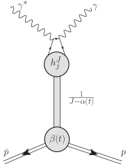
Concerning the dependence on , the partial wave amplitudes are modelled by relying on a Regge-inspired picture of -channel exchanges of mesonic states of total angular momentum which are
-
•
coupled with strength parameter to quark-antiquark state (formed at short distance by colliding photons),
-
•
propagating as appropriate Reggeon
(97) with trajectory
(98) -
•
and which is coupled to nucleon–anti-nucleon pair with strength described by a -pole impact form factor
(99) parameterized by cut-off mass (not to be confused with proton mass), giving the total Ansatz
(100)
This is illustrated on fig. 2. Using again the simple PDF ansatz of eqs. (94-96), and restoring full Regge trajectory as in eq. (98), one gets for the leading partial wave amplitude
| (101) |
In some studies, the residual dependence on has been described by an exponential ansatz , often used in Regge phenomenology, instead by a multipole impact form factor eq. (99). Such an exponential ansatz brings no advantage in fits to present data and is more difficult to advocate from field-theoretic perspective, so a multipole ansatz is favored. Note that the cut-off mass parameter could also in principle depend on angular momentum, , but the additional parametrization describing this also brings no advantage in fits so this is presently usually ignored.
Modelling of all GPDs relevant for present phenomenology within the framework of full Mellin-Barnes SO(3) partial wave decomposition has not yet been undertaken. Models presently on the market truncate the SO(3) series eq. (91) to one or few leading terms, i.e. terms with highest , corresponding to smallest powers of . Furthermore, these models were originally devised for description of small- collider DVCS data so further expansion around was made to obtain simplified model of form Kumericki:2007sa ; Kumericki:2009uq
| (102) |
where and dependence of subleading partial waves is for simplicity taken to be equal to that of leading one, i.e., given by eq. (101). Strength of subleading partial waves are free parameters of the model. They essentially control the skewness property of the GPD, i.e. the ratio of the GPD on the so-called crossover line and GPD at . Since the normalization parameter and the Regge intercept are fixed by DIS data, the -dependence of , and thus that of the GPD, is controlled by and the cut-off mass . In the singlet sector, relevant for small- region, the values are fixed. Such values are favored by fits, but fits are not very sensitive to them, so leaving them as free parameters proved inefficient. Cut-off masses are in present fits strongly correlated with values of multipole power in eq. (99), so it makes sense to also fix values for . Counting rules would give and , but to facilitate direct comparison of the cut-off mass with the characteristic proton size coming from the dipole parametrization of Sachs form factors, one can take . Fits are also not sensitive to the gluon cut-off mass , which can be fixed at , value suggested by the analysis of production collider data Aktas:2005xu . This leaves the final set of free model parameters:
| (103) |
for models of sea quark and gluon GPDs with three partial waves, (sometimes called nnl-PW) used in newest published fits Kumericki:2013br . In ref. Kumericki:2009uq two partial waves (nl-PW) are used. The third partial wave does not bring much more flexibility to fits but the resulting gluon GPDs turn out to be more realistic considering their partonic interpretation (fits without third wave tend to have negative gluon GPD at low ). The inclusion of second partial wave is, however, essential. Namely, the skewness ratio of the minimal, leading partial wave model (l-PW) is fixed at a too large a value to describe simultaneously DIS and DVCS data. The described models (with two or more partial waves) can successfully reproduce all available low- DVCS data, see sec. 2.7.1. They are also used as a sea parton component of hybrid models Kumericki:2009uq , where the valence component is described by the simpler modelling of just the GPD on the crossover line , and using dispersion relation technique, see sec. 2.4, to recover the remaining needed part. As described in sec. 2.7.1, such hybrid models are able to describe essentially all presently available DVCS data.
1.5.3 Spectator models
GPD spectator models are specific applications of the covariant scattering matrix approach (sec. 1.4.2) stemming from a more phenomenological view of the problem, or from a bottom-up perspective.
In these models the parton-proton amplitude is described by a holomorphic function which exhibits four poles in the complex plane. GPDs in the DGLAP region, , are determined by the -channel simple pole from the spectator propagator; conversely, in the ERBL region, , they are obtained setting either quark on-shell, i.e. from the two poles in the proton-quark vertex functions.
In ref. Brodsky:2008qu a model for the GPD was given for a scalar diquark spectator, where the vertex functions reproduce the perturbative asymptotic behavior of the Dirac form factor, . This model is by construction “hard”, and it does not reproduce the electromagnetic form factor behavior at small momentum transfer. However, a set of parameters is provided which give the correct normalization, , while providing functional forms for the GPD behavior at different values of .
A more general version of the perturbative diquark model was given in refs. Goldstein:2010gu ; GonzalezHernandez:2012jv ; Ahmad:2006gn ; Ahmad:2007vw ; Goldstein:2013gra which includes a Regge-inspired spectral analysis for the parton-proton scattering amplitude. This resulted in a parametric form for the DGLAP region based on a “Regge improved” diquark model, or “reggeized diquark model”, that also provides a framework for reproducing the low behavior of the proton form factors. The ERBL region is treated in this model so that the properties of crossing symmetry, continuity at the crossover points with the DGLAP region () and approximate polynomiality are satisfied. Regge behavior is obtained by letting the spectator system’s invariant mass, , vary according to a spectral distribution, at variance with most models where the recoiling system’s mass is kept fixed. The variable mass spectator systems exhibit different structure as one goes from low to high mass values: at low mass values one has a simple scalar or axial vector spectator, whereas at large mass values one has more complex correlations. The occurrence of the latter, also known as reggeization ref. GonzalezHernandez:2012jv , is regulated by a spectral distribution, which upon insertion in the correlation function yields for small the desired behavior. The resulting parametrization was summarized in the following expression for the quark sector,
| (104) |
where , ; the functions , and , are the quark-diquark and Regge contributions, respectively. They depend on mass parameters for: the struck quark, , the (diquark) spectator, , the diquark form factor cut-off parameter, . The Regge trajectory parameters are: (intercept), (slope), and (x-dependent modulation).
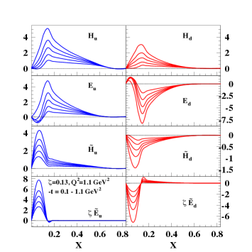
The parametrization can be extended to the valence quark, sea quark, and gluon contributions. For valence quarks the spectator is given by scalar and axial-vector diquarks, which, through the symmetry, allow one to perform a flavor analysis by distinguishing between isoscalar () and isovector () spectators. For scattering from sea quarks, the spectator is a tetra-quark state, namely a state with . For gluons it is a three quark system in a color octet state. The possibility of distinguishing among different flavors in this model reflects the underlying color symmetry which can be seen as an indirect manifestation of chiral symmetry breaking.
The set of chiral even GPDs, from the model is shown in fig. 3. The quark-diquark components are given by,
| (106) | |||||
| (108) | |||||
where , , and , the incoming and outgoing quark virtualities, depend on , , and ; , the normalization constant, is in 4. Although the parametrization is written for the “asymmetric” choice of kinematics with the initial proton momentum along the -axis, this can easily be connected to the “symmetric” choice, adopted in our review, where the average of the initial and final proton momenta are along ref. Diehl:2003ny . The Regge term is given by
| (109) |
where
| (110) |
A quantitative fit using experimental information from DIS, the nucleon electroweak form factors, and a selection of available DVCS data from Jefferson Lab Girod:2007aa was developed using the valence component of the parametrization in ref. Goldstein:2010gu : the model is consistent with theoretical constraints imposed numerically, and the experimental data are let to guide the shape of the parametrization as closely as possible.
2 Theoretical and experimental status
2.1 Theory of DVCS
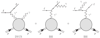
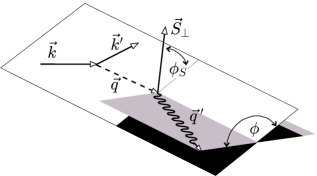
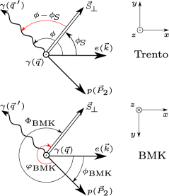
Measurements of DVCS are mostly realized via the process of leptoproduction of a real photon, where also an interference with the Bethe-Heitler radiation occurs, as displayed in fig. 4. The general cross-section is differential in , the negative squared momentum of virtual photon , the squared momentum transfer , and two azimuthal angles measured relatively to the lepton scattering plane: the angle to the photon-target scattering plane and the angle to the transversal component of the target polarization vector, as displayed on fig. 5. The cross section is given by
| (111) |
where is the electromagnetic fine structure constant, , is the mass of the target, and is coherent superposition of DVCS and Bethe-Heitler amplitudes
| (112) |
The DVCS amplitude can be decomposed either in helicity amplitudes or, equivalently, in complex valued Compton Form Factors (CFFs) which are to be measured in experiments. The latter are usually denoted as
Owing to the validity of QCD factorization theorems Collins:1998be the CFFs can be written at leading order in perturbative QCD, as the following convolution (),
| (113) | |||||
| (114) | |||||
where the choice of symbols is motivated by their relation to GPDs. As a consequence of helicity conservation at the photon vertex, the transversity GPDs appear only at NLO in DVCS. They can be measured, however, in processes that directly allow for helicity flip, for instance in and production Ahmad:2008hp . In particular, electroproduction constitutes the main background process for DVCS. In the experimentally accessible range of , power corrections can be relatively large; for these the formalism is extended to include a set of higher twist GPDs and CFFs denoted . The transversity gluon GPDs also appear at this order Belitsky:2001ns . It should be noted that the literature does not provide a uniform naming scheme for the twist three GPDs: three different notations appear in refs. Belitsky:2001ns ; Meissner:2009ww ; Kiptily:2002nx , respectively. A conversion table among schemes for the vector sector was given in ref. Courtoy:2013oaa . Finally, a recent analysis of twist four corrections including kinematic power corrections and in terms of double distributions and Mellin-Barnes integrals has been recently made available in ref. Braun:2014sta .
The nonperturbative part of the Bethe-Heitler amplitude is, on the other hand, given in terms of the (in the relevant kinematical region) well-known elastic form factors and . This then, through the interference term , gives an experimental access to both the real and imaginary parts of the CFFs.
The various CFFs/GPDs can be disentangled by measuring several independent observables in exclusive lepton–proton scattering experiments where both the lepton beam and the target can be polarized. The general framework is given in terms of helicity amplitudes for the process, as described e.g. in ref. Diehl:2005pc . These in turn factor into a hard scattering amplitude for the process, , , which depends on the initial and final photon and quark helicities, and a quark-proton helicity amplitude , which contains the GPDs. In DVCS, in particular, only the chiral even GPDs can be tested.
The helicity structure of the GPDs is described systematically in ref. Diehl:2003ny . At twist two the relevant amplitudes are,
| (115) | |||||
| (116) | |||||
| (117) | |||||
| (118) |
The remaining helicity configurations are obtained by parity relations: . The phase factor contains the angle between the lepton and hadron planes (see fig. 5). Using products of the helicity amplitudes to form the various contributions to the cross sections in eq. (112), one obtains an expression that depends on various modulations of the type , and . The final expressions provided in ref. Belitsky:2001ns read,
| (119) |
| (120) |
| (121) |
where is the lepton energy loss in the target frame, in eq. (120) is the lepton beam charge in units of positron charge, and originate from the lepton propagators in Bethe-Heitler amplitude (see ref. Belitsky:2001ns for expressions). The CFFs enter quadratically the harmonic coefficients and of , and linearly those of , while they don’t enter the (often dominant) Bethe-Heitler squared part. Detailed expressions for the coefficients and are given in refs. Belitsky:2001ns ; Belitsky:2008bz ; Belitsky:2010jw ; Belitsky:2012ch , labeled BMK. Note that the cross section in eq. (111) undergoes a similar decomposition into its BH, DVCS and interference terms whether the target is unpolarized, longitudinally polarized, or transversely polarized, the coefficients and being given by different expressions with sensitivities to different GPDs in each case.
One should keep in mind that BMK use a different coordinate system, which is related to the “Trento” coordinate system of fig. 5 by
| (122) | ||||
| (123) |
see fig. 6.
One of the biggest challenges in DVCS analyses is a precise determination of the dependence of the various asymmetries and/or cross section terms from which to extract the CFFs. As we explain in the following sections, these are particularly hard to disentangle in asymmetry measurements, since they contain “competing” -dependent terms both in the numerator and denominator of their expressions. Among the harmonic coefficients in eqs. (120-121) the ones which are expected to be dominant because they contain leading twist GPDs are
Each coefficient has a different form depending on the target polarization and is dominated, in turn, by a specific GPD. The coefficient is particularly interesting, even if non leading, because it has been singled out as a direct probe of the twist-three GPD which measures orbital angular momentum Courtoy:2013oaa . Finally, for BH, are dominant, the rest of the coefficients being suppressed by kinematics.
2.2 DVCS observables
To access particular CFFs via leptoproduction measurements, one uses some kind of harmonic analysis and various choices of beam and target polarizations and charges, if available.
Using the notations of ref. Kroll:2012sm , the cross section for the leptoproduction of a real photon by a lepton (with charge in units of the positron charge, and helicity ) off an unpolarized target can be written as
| (124) |
where only the -dependence of the observables is explicit. In facilities where longitudinally polarized, positively and negatively charged beams are available, the asymmetries , and can be isolated. This is the case for a large part of HERMES data, see sec. 2.5. It is quite conventional to use the first subscript to refer to the beam and second to the target polarization ( for unpolarized, for longitudinal, etc.). For example, the beam charge asymmetry is singled out from the combination
| (125) |
Analogous combinations yield the two beam spin asymmetries and :
| (126) | |||||
| (127) |
If an experiment has access to only one value of , such as in Jefferson Lab, the asymmetries defined in eq. (124) cannot be isolated. One can only measure the beam spin asymmetry , which depends on the combined charge-spin cross section as
| (128) |
In this equation we use the usual notation of labelling the combined charge-spin cross section with the sign of the beam charge and an arrow () for the helicity plus (minus). can be written as a function of the asymmetries defined in eq. (124)
| (129) |
The target longitudinal spin asymmetry reads
| (130) |
where the double arrows () indicates the target polarization state parallel (anti-parallel) to the beam momentum. The double longitudinal target spin asymmetry is defined similarly
| (131) |
The HERMES collaboration also had access to a transversely polarized target with both electrons and positrons. They therefore were able to measure two types of observables
| (132) |
| (133) |
where dependence on is suppressed on RHS.
For experiments which cannot deliver cross-sections, but asymmetries, one can often use the dominance of the Bethe-Heitler term in the denominator to still obtain more or less direct linear dependence on CFFs. For example, the first sine harmonic of the beam spin asymmetry, as measured e.g. in Jefferson Lab, is defined as
| (134) |
This harmonic is then approximately proportional to linear combination of CFFs:
| (135) |
and will be dominated by . Similarly, beam charge asymmetry gives access to etc.
If one measures cross-sections, one can also perform normal Fourier analysis, or it may be favorable to work with specially weighted Fourier integral measure Belitsky:2001ns
| (136) |
thus cancelling strongly oscillating factors in Bethe-Heitler and interference terms, eqs. (119-120). Series of such weighted harmonic terms, e.g.
| (137) |
converges then faster with increasing than normal Fourier series.
2.3 Evaluation of Compton Form Factors
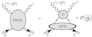
For the twist-two related first four CFFs () we have a factorization theorem Collins:1998be , see fig. 7, expressing them to leading order in as convolution of the perturbatively calculable hard-scattering coefficient and the non-perturbative GPD function, e.g., for flavor singlet () contribution,
| (138) |
where is the factorization scale, usually set equal to photon virtuality , and to the LO scaling variable is
| (139) |
Here we organize the singlet quark and gluon GPDs in a column vector
| (140) |
and the hard scattering coefficient functions in a row vector,
| (141) |
whose QCD perturbation series starts as
| (142) |
Note that the crossed-diagram contribution to eq. (142) is absorbed into the symmetrized quark singlet distribution
| (143) |
where the upper sign in the bracket is valid for , while lower is for . Formulas for the non-singlet sector are analogous, and the total CFF is
| (144) |
with charge factors and determined using the decomposition of sum over active light quark flavors
| (145) |
so that in LO the familiar “handbag” approximation formulas eqs. (113-114) are recovered.
If one is working in the conformal moment GPD representation, see sec. 1.4.4, factorization formula for CFFs (138) can be transformed in the space of conformal moments using transforms (66–67) for GPDs and transforms
| (146) |
for coefficient functions. Then eq. (138) is transformed into a divergent infinite sum
| (147) |
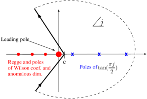
We can resum it using the Mellin-Barnes integration along the complex- plane contour shown on fig. 8 and (with the help of dispersion relations connecting real and imaginary part of CFF) we get
| (148) |
In the conformal moments approach, evolution of GPDs from some fixed input scale to the scale of interest is given by
| (149) |
where evolution operator mixes gluon and singlet quark components but is diagonal () at LO, and in the special scheme also at NLO. Explicit form of this operator (including diagonal NNLO part) for non-singlet and singlet case can be found in refs. Mueller:2005nz ; Kumericki:2006xx ; Kumericki:2007sa .
2.4 Dispersion relation technique
Using analytic properties of the DVCS amplitude via dispersion relations provides a convenient modelling tool Frankfurt:1997ha ; Teryaev:2005uj ; Kumericki:2007sa ; Anikin:2007yh ; Diehl:2007jb ; Polyakov:2007rv . Note that since GPDs are real functions, the handbag formula eq. (113) leads to a simple LO relation between the GPD calculated at the cross-over line and the imaginary part of the CFF, e.g., for ,
| (150) |
On the other hand, the dispersion relation connects this to ,
| (151) |
and at the most one subtraction constant
| (152) |
Instead of one can model the simpler functions and , in a LO and leading-twist approximation, ignoring the effects of GPD evolution, which are all acceptable approximations when trying to describe presently available data in fixed-target kinematics (for a critique of the use of dispersion relations beyond LO, see Goldstein:2009ks .) The dispersion relation technique has been utilized in Kumericki:2009uq for modelling the valence part of GPDs in hybrid models, see sec. 2.7.1.
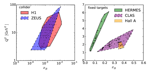
2.5 Existing experimental data
We will not go into a detailed review of DVCS experiments, but will just display a simple overview of available data on proton targets in the form of tables 4 and 5. The current kinematic coverage is summarized in fig. 9.
| Collab. | Year | Ref. | Observables | Kinematics | No. of points | ||||
|---|---|---|---|---|---|---|---|---|---|
| [2] | [] | [2] | total | indep. | |||||
| H1 | 2001 | Adloff:2001cn | , , , | 2–20 | 30–120 | 1 | 4+4 4+4 | 4 | |
| ZEUS | 2003 | Chekanov:2003ya | , , | 5–100 | 40–140 | 10+13 12 | 13 | ||
| H1 | 2005 | Aktas:2005ty | , , | 2–80 | 30–140 | 1 | 9+14 12 | 9 | |
| H1 | 2007 | Aaron:2007ab | , , | 6.5–80 | 30–140 | 1 | 4+5 15 48 | 15 24 | |
| ZEUS | 2008 | Chekanov:2008vy | , , | 1.5–100 | 40–170 | 0.08–0.53 | 6+6 8 4 | 8 | |
| H1 | 2009 | Aaron:2009ac | , , , | 6.5–80 | 30–140 | 1 | 4+5 15 24+6 | 15 6 | |
| Collab. | Year | Ref. | Observables | Kinematics | No. of points | ||||
|---|---|---|---|---|---|---|---|---|---|
| [2] | [2] | total | indep. | ||||||
| HERMES | 2001 | Airapetian:2001yk | 0.11 | 2.6 | 0.27 | 1 | 1 | ||
| CLAS | 2001 | Stepanyan:2001sm | 0.19 | 1.25 | 0.19 | 1 | 1 | ||
| CLAS | 2006 | Chen:2006na | 0.2–0.4 | 1.82 | 0.15–0.44 | 6 | 3 | ||
| HERMES | 2006 | Airapetian:2006zr | 0.08–0.12 | 2.0–3.7 | 0.03–0.42 | 4 | 4 | ||
| Hall A | 2006 | MunozCamacho:2006hx | , | 0.36 | 1.5–2.3 | 0.17–0.33 | 424+1224 | 424+1224 | |
| CLAS | 2007 | Girod:2007aa | 0.11–0.58 | 1.0–4.8 | 0.09–1.8 | 6212 | 6212 | ||
| HERMES | 2008 | Airapetian:2008aa | , , , | 0.03–0.35 | 1–10 | 0.7 | 12+12+12 12+12 12 | 4+4+4 4+4 4 | |
| CLAS | 2008 | Gavalian:2008aa | 0.12–0.48 | 1.0–2.8 | 0.1–0.8 | 66 | 33 | ||
| HERMES | 2009 | Airapetian:2009aa | , , | 0.05–0.24 | 1.2–5.75 | 0.7 | 18+18+18 18+18+18+18 | 6+6+6 6+6+6+6 | |
| HERMES | 2010 | Airapetian:2010ab | , | 0.03–0.35 | 1–10 | 0.7 |
12+12+12
12+12+12 |
4+4+4
4+4+4 |
|
| HERMES | 2011 | Airapetian:2011uq | , , , | 0.03–0.35 | 1–10 | 0.7 |
12+12+12
12+12 12+12 12 |
4+4+4
4+4 4+4 4 |
|
| HERMES | 2012 | Airapetian:2012mq | , , | 0.03–0.35 | 1–10 | 0.7 |
18+18+18
18+18+18+18 |
6+6+6
6+6+6+6 |
|
| CLAS | 2015 | Pisano:2015iqa | , , | 0.17–0.47 | 1.3–3.5 | 0.1–1.4 | 166+166+166 | 166+166+166 | |
| CLAS | 2015 | Jo:2015ema | , | 0.1–0.58 | 1–4.6 | 0.09–0.52 | 2640+2640 | 2640+2640 | |
| Hall A | 2015 | Defurne:2015kxq | , | 0.33–0.40 | 1.5–2.6 | 0.17–0.37 | 480+600 | 240+360 | |
2.6 Fitting methods
In a perfect world, one would like to be in possession of several well-motivated GPD models, depending on a small number of parameters which have one-to-one correspondence to physical properties of the nucleon, and one would perform a simple global fit of this model(s) to all available data, with global minimum of (or related goodness-of-fit estimator) revealing the GPD-encoded nucleon structure. Having several models relying on qualitatively different dynamical descriptions allows one to make robust — or discriminating — predictions for future experiments, and to evaluate accurately the needed beam time. It also permits stringent tests of fitting techniques through fits to pseudo-data, generated by one model, and analysed with another one.
A similar approach, or global fitting, has been working out fine for PDFs, where results of several groups, using different methods on different data sets are generally in good agreement, or they can be compared to one another including their uncertainties. These results are extremely useful for the whole high-energy physics community. So naturally, one hopes that the extraction of GPDs could follow in these footsteps. True, there are more GPD functions to be determined then there are PDFs, but there are also more observables to be measured, even considering only DVCS, thanks to the final state exclusivity (neglecting, for the sake of argument, intrinsic difficulties of exclusive measurements compared to inclusive ones). This has been beautifully illustrated by HERMES measurements of the almost complete set of DVCS observables. Next, going from measurements to GPDs involves some sort of deconvolution of factorization formula eq. (138), which is widely considered a major obstacle in determination of GPDs. But one should keep in mind that PDFs are also convoluted almost exactly the same way!
A more serious hurdle is dealing with the dimensionality of the domain space of the unknown functions: three dimensions for GPD in comparison to just one for PDF , if we consider the dependence on the factorization scale, , to be known (therefore not listed among the arguments of the functions in this context). This situation is well known in the field of data analysis as the curse of dimensionality333“It is easy to find a coin lost on a 100 meter line, but difficult to find it on a football field.” Here we could say that we deal with a haystack, 100 m per side.. As the dimensionality of the domain space increases, any amount of available data becomes exponentially sparse. So it is overly optimistic to expect any time soon in GPD physics a situation like the present one with unpolarized PDFs. We have an excellent knowledge of these functions in a wide range of their and domains, from fits to experimental data carried out in the course of several decades, using a variety of functional forms and approaches including the neural networks, which have been accurately benchmarked so as to be readily comparable to one another. Note in this context that all known constraints on the GPDs, listed in sec. 1.3, result in the reduction of flexibility in choosing a GPD functional form, or a reduction in volume of domain space, without providing any help with the problem of dimensionality. However, this situation will significantly improve in the near future, with the release of GPD-related data of unprecedented accuracy, in particular from Jefferson Lab. Even if not matching the accuracy and sophistication of PDF fits, highly precise data will bring the GPD field closer to the current mapping of PDFs. A careful look at the present situation, and a series of recommendations, will hopefully help bridging this gap faster.
Even more than in the case of PDFs, the success of any attempt of global GPD fitting depends on the choice of the fitting function, or GPD model. This also means that the choice of the model introduces a significant bias, which is difficult to estimate quantitatively, and care has to be exercised when stating uncertainties of fitting results. Taking the model parameter errors determined by observing the variation of with their change, results in an error band that only renders a partial representation of the uncertainty from the comparison of experiment with any particular fitting procedure, but it does not account for the entirety of the theoretical uncertainty, or what we could dub as theory “systematics”.
As will be reviewed in sec. 2.7, global fits existing in the present literature are reasonably successful and it looks like there are no major problems with the described theoretical framework. Still, many challenges lie ahead that will be important as forthcoming high-precision data from Jefferson Lab upgraded at 12 , COMPASS II, and, further down the road, from an EIC, become available. These include requiring that the various models and fits describe simultaneously both the unpolarized and polarized target data, as well as meson production data with terms beyond leading twist. A subsequent step will also include a more detailed analysis of the dependence of the data on , which will include going beyond LO of the QCD perturbation series. Data from the deuteron and other nuclear targets will also be available for global fits, and will allow for a precise flavor separation of the various GPDs. Because of this, other fitting approaches have also been tested, such as various versions of the so-called local fits, and fits using neural networks.
Local fits utilize the fact that several observables can be measured at a single kinematical point. Then one can search for values (as opposed to shapes) of CFF functions that can describe the data at this point or in its close vicinity. In that respect, local fits correspond to CFF sampling. Such a procedure can in principle be free of the serious model biases of global fits, since so far it relies essentially on a leading-twist handbag formalism. As exemplified with eq. (135), there are well-established relations between the CFFs and the DVCS observables. These relations depend only on kinematical factors, or on the now well-known (or well enough for our purpose) nucleon form factors. At a given () experimental point, these factors can be determined and the procedure thus consists, for each such experimental point, in fitting simultaneously the various observables available for this particular kinematics, taking the real and imaginary parts of CFFs as free parameters. In principle real and imaginary parts are related by dispersion relation such as eq. (151). However, the lack of data, and the smallness of the physical region which gives access only to a sub-interval of the integration domain, has been preventing so far the implementation of dispersion relations in local fits.
As already stressed, the main advantage of the local fits is that they are almost model-independent (in the limit that the leading-twist assumption is correct), as the CFFs can vary freely. The main shortcoming is that CFFs are fitted, and not GPDs themselves. At LO, the imaginary part of a CFF is equal to singlet and non-singlet GPD combinations (27) evaluated at , but beyond LO this simple interpretation is lost. Therefore, in order to access GPDs, carrying out an additional model-dependent deconvolution (similar to a global fit) seems unavoidable. Nevertheless, in the light of the complicated interplay of many observables and many GPDs that can be difficult to disentangle in the global fitting procedure, local fits can provide quite direct information about nonperturbative structure functions in a given kinematical– region, and can serve as a good consistency check of the whole framework. They can also be considered as a first (although not mandatory) step towards GPDs.
Another approach to the extraction of GPDs from data is to harness some of the fast increasing number of machine learning techniques, for example Artificial Neural Networks (ANN). The latter are designed to recognize structure in a given data set and to quantify the statistical properties of this structure. They have already been successfully applied to the task of fitting hadronic structure functions to the data, for standard PDFs Forte:2002fg ; Ball:2008by , or electromagnetic form factors Graczyk:2014coa . It is a mathematical theorem that neural networks are able to approximate any smooth function cybenko89 , so they can be used as a GPD model without danger of introducing bias from the model parameters. Fitting neural networks to replicas of experimental data gives a convenient method of propagating (correlated and uncorrelated) experimental uncertainties into GPDs. Combined with the aforementioned lack of modelling bias, this suggests that neural networks are a promising method for obtaining GPDs with a realistic, or faithful uncertainty estimate which certainly deserves further studies.
ANN-based approaches have not yet been applied specifically to quantitative fits of GPDs, but only of CFFs (see the preliminary study in ref. Kumericki:2011rz ). Many open questions remain at present, for instance how to implement some of the GPD properties from sec. 1.3 in this framework, or how to handle the problem of the large dimensionality of the space of unknown functions.
An intermediate and more affordable goal would be that, in a spirit similar to the local fits, an ANN-based approach could render a parametrization of the CFFs. ANN used for this intermediate step of the analysis would provide useful information in the form of a representation of experimental data which is closer to the sought-after GPDs than the actual observables. This information could then be used in searches for flexible-enough GPD models to be used in traditional fitting procedures.
It is also important to notice that different forms of ANN-based algorithms are possible, and that subclasses of specific algorithms could work more appropriately for the complex multi-variable problem of GPD fitting. For instance, an alternative to the standard ANN approaches was developed in refs. Honkanen:2008mb ; Askanazi:2014gxa for PDF fits using Self-Organizing Maps (SOM). A most important aspect of self-organizing algorithms is in their ability to project high dimensional input data onto lower dimensional representations while preserving the topological features present in the training data. This aspect makes the SOM algorithms particularly appealing for an application to future GPD fitting.
2.7 Fits to the data
The different types of fits described above have been applied to a variety of data sets, following different procedures. Only a few groups have attempted to extract information using directly DVCS data. In the global fit sector we list KM Kumericki:2007sa ; Kumericki:2009uq ; Kumericki:2013br , GK Goloskokov:2007nt (where fit was to DVMP data, but provides reasonable description of DVCS as well), and GGL Goldstein:2010gu . Local fits were performed in refs. Guidal:2008ie ; Moutarde:2009fg ; Guidal:2009aa ; Guidal:2010ig ; Guidal:2010de ; Kumericki:2013br ; Boer:2014kya . Finally a first application of an ANN based fit to GPDs was given in ref. Kumericki:2011rz . As we discuss later on, the fitting procedures that were used so far are candidates for future more extensive data analyses, once subjected to an appropriate benchmarking. In what follows we describe in more detail the various efforts to analyse data both globally and locally.
2.7.1 Global fits
Global fits restricted to low- collider data
First fits using Mellin-Barnes SO(3) partial wave expansion model described in sec. 1.5.2 were performed in Kumericki:2007sa , where only the leading partial wave of eq. (102) was used (so GPD doesn’t depend on ). For such rigid model the quark GPD skewness ratio
| (153) |
(where denominator is calculated using the corresponding PDF, see eq. (18)) is fixed at its conformal (“Shuvaev”Shuvaev:1999ce ) value
| (154) |
which is too large to correctly describe DVCS data at LO, where these data point to . (By the way, it turns out that at NLO the conformal value (154) of skewness ratio is more realistic.)
Adding second partial wave, with negative values of skewness parameters and , enabled successful simultaneous description of HERA collider DIS and DVCS data, at LO, NLO ( and scheme) and NNLO ( scheme) Kumericki:2009uq . These fits to 85 DIS and 101 DVCS data points (where not all were statistically independent) consistently had . Choice to directly fit also to DIS measurements and not to use some standard published PDFs was motivated by wish to work within a consistent framework for description of both processes, including relatively simple prescription for treatment of heavy flavors (i.e., ignoring them), where fixed number of light quarks was used.
Let us also mention that the first attempt of a global fit that besides DVCS includes also exclusive electroproduction of and mesons is described in ref. Lautenschlager:2013uya . This complements the fits carried out through a decade, based on several variants of the hand-bag model by GK Goloskokov:2007nt for the description of deeply virtual meson production.
Global fits restricted to fixed target data
Jefferson Lab 6 fixed target experiments have afforded us several high precision data sets in a kinematic region characterized by larger values and in the multi- range, where valence quark distributions are expected to dominate (see fig. 9). Even so, DVCS data alone are not sufficient to reliably extract GPDs from data, and complementary information from both exclusive measurements (nucleon form factors) and DIS (PDFs) needs to be utilized. How to practically use this information is open to question and several groups have proposed different approaches. We refer in particular to GK which use the hand-bag model within the double distribution ansatz Goloskokov:2007nt , Diehl and Kroll who performed a quantitative zero-skewness GPD extraction based entirely on form factors data and PDFs from DIS Diehl:2013xca , and GGL who introduced a recursive fit based on the reggeized diquark model to organize information from the inherently different types of data sets Goldstein:2010gu . We give a more detailed description of the latter since it provides a flexible approach with tunable parameters affording a quantitative phenomenological extraction of GPDs from data including the evaluation of the theoretical uncertainty. The initial evaluations in ref. Goldstein:2010gu are usable templates for future fits including a more extended set of data. Results from this parametrization are summarized in table 6. The recursive procedure works as follows: in a first phase one fits the forward limit of the GPDs and , given by PDFs from unpolarized and polarized DIS scattering, using only valence distribution functions. In this step the mass parameters , , , the Regge parameter, , as well as the normalization factors for and , eqs. (LABEL:GPDH,1.5.3), are determined. In ref. Goldstein:2010gu it was chosen not to quote an error on these parameters because parametrizations of the valence components of PDFs, not the actual data, were used in the fit. The parameters, , , are subsequently obtained, as well the normalizations for , and by fitting the proton and neutron electromagnetic form factors, and the axial and pseudoscalar form factors, respectively (eqs. (28,29)). A very large number of data sets on the nucleon form factors is available. The sets that were used are listed in refs. Goldstein:2010gu ; GonzalezHernandez:2012jv ; Ahmad:2006gn ; Ahmad:2007vw . Finally, the dependence on the skewness variable, , is determined by fitting the parameters that determine the shape of the ERBL () region with the set of data on .
| u quark | ||||
|---|---|---|---|---|
| PDFs Fit | ||||
| (GeV) | 0.420 | 0.420 | 2.624 | 2.624 |
| (GeV) | 0.604 | 0.604 | 0.474 | 0.474 |
| (GeV) | 1.018 | 1.018 | 0.971 | 0.971 |
| 0.210 | 0.210 | 0.219 | 0.219 | |
| Nucleon Form Factors Fit, 177 points Ahmad:2006gn | ||||
| 2.448 0.0885 | 2.811 0.765 | 1.543 0.296 | 5.130 0.101 | |
| 0.620 0.0725 | 0.863 0.482 | 0.346 0.248 | 3.507 0.054 | |
| 2.043 | 1.803 | 0.0504 | 1.074 | |
| /d.o.f. | 0.773 | 0.664 | 0.116 | 1.98 |
| d quark | ||||
| PDFs Fit | ||||
| (GeV) | 0.275 | 0.275 | 2.603 | 2.603 |
| (GeV) | 0.913 | 0.913 | 0.704 | 0.704 |
| (GeV) | 0.860 | 0.860 | 0.878 | 0.878 |
| 0.0317 | 0.0317 | 0.0348 | 0.0348 | |
| Nucleon Form Factors Fit, 177 points Ahmad:2006gn | ||||
| 2.209 0.156 | 1.362 0.585 | 1.298 0.245 | 3.385 0.145 | |
| 0.658 0.257 | 1.115 1.150 | 0.974 0.358 | 2.326 0.137 | |
| 1.570 | -2.800 | -0.0262 | -0.966 | |
| /d.o.f | 0.822 | 0.688 | 0.110 | 1.00 |
Global world data fits
To fit all available DVCS data (coming from both collider and fixed-target experiments) in refs. Kumericki:2009uq ; Kumericki:2013br hybrid modelling approach was used, where the sea parton part is modelled by Mellin-Barnes SO(3) partial wave expansion conformal space models described in sec. 1.5.2 (including LO QCD evolution), while the valence part is modelled using the dispersion relation technique described in sec. 2.4 (where PQCD evolution is ignored). In particular, the valence part of and GPDs is modelled at the cross-over line using a diquark-inspired model
| (155) |
(and similarly for ) where normalization of the corresponding PDF (, ) is factored out so that the free parameter corresponds to the skewness ratio eq. (153). Free parameters and control large- and residual dependence, respectively. For , the Regge trajectory is used,
| (156) |
This GPD gives the imaginary part of the CFF (see eq. (150)), and the dispersion relation (151) gives the corresponding real part, apart from the subtraction constant which is separately modelled like
| (157) |
giving two additional free parameters, and . In refs. Kumericki:2009uq ; Kumericki:2013br GPD is modelled solely in terms of this subtraction constant, i.e., , while contribution of GPD is described using pion-pole-inspired effective ansatz
| (158) | ||||
| (159) |
where , while and are free parameters.
In total, the hybrid models used in global fits have 11-18 free parameters. Table 7 gives an overview of various instances of the published fits with their characteristics and a list of the measured observables that were used. Fits are multi-step, as denoted by braces and parentheses in the table. Thus, for example, for the model KM09a first a three-parameter (, , ) fit to 85 DIS data points is performed, fixing the leading SO(3) partial wave at in (96). Second, the three-parameter (, , ) fit to 45+56=101 and collider measurements is done fixing the shape of sea-quark and gluon GPDs. Finally, a five-parameter (, , , , ) fit to 36 fixed-target beam spin and charge asymmetries fixes the valence part of the model. Preliminary fit to DIS (and for KM09a and KM09b also second preliminary fit to collider DVCS data) is always with or better, and only the of the final fit is displayed in the table.
As can be seen from table 7, most of the KM global fits have used only data coming from measurements on unpolarized target, which was what the just described hybrid model was designed for. The principal difference between various instances of KM09 and KM10 models is in their treatment of cross-section measurements by Hall A collaboration MunozCamacho:2006hx . Models KM09a and KM10a don’t use this data at all, whereas KM09b and KM10b use the ratio of and weighted cosine harmonics, see eq. (137). Model KM10 and newest published KMM12 model directly use all available non-zero harmonics of Hall A data from ref. MunozCamacho:2006hx , and KMM12 experimentally adds also polarized target data. KM10a,b models are an update of KM09a,b models, where for KM09x sea-quark and gluon GPD components were pre-fitted to the collider subset of data, while for KM10x and KMM12 true simultaneous global DVCS fit was performed.
Special treatment of Hall A data was necessary because of its extreme precision, posing quite a challenge for models, especially with the size and strong -dependence of the unpolarized cross-section. To come to terms with that, KM10 model has extremely large contribution which is considered an effective parametrization of some large contribution to DVCS amplitude. Such a large leads to a conflict with measurements on longitudinally polarized target, so KMM12 model, which included also data, had to have some other way to deal with the Hall A data. It was accomplished by simultaneous increase of both and pion-pole contributions.
In the meantime, Hall A collaboration updated their measurements of electroproduction cross-section in ref. Defurne:2015kxq . Change with respect to 2006 data MunozCamacho:2006hx is significant and it looks like this updated data will be easier to describe with existing models. Indeed, the recent model KM15 from ref. Kumericki:2015lhb , obtained by adding also the 2015 data coming from Hall A Defurne:2015kxq and CLAS Pisano:2015iqa ; Jo:2015ema collaborations to the fit, releases some tensions present in older fits.
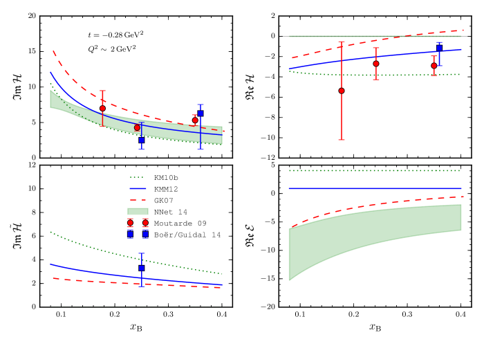
2.7.2 Local fits
In the following we describe the efforts Guidal:2008ie ; Moutarde:2009fg ; Guidal:2009aa ; Guidal:2010ig ; Guidal:2010de ; Moutarde:2009fg ; Kumericki:2013br ; Boer:2014kya towards CFF fitting with different approaches that can all be seen as variations around the local fit strategy.
Least squares minimization
This method was pioneered in 2008 Guidal:2008ie . In refs. Guidal:2008ie ; Guidal:2009aa ; Guidal:2010ig ; Guidal:2010de , only seven parameters were considered: , , , , , and , and was fixed to 0. This assumption has been recently removed Boer:2014kya . Real and imaginary parts of CFFs were free to vary within a 7- or 8-dimensional hypervolume, bounded by rather conservative limits: 5 times the predictions of the VGG model.
Local fits of CFFs are usually underconstrained problems. For example, let us consider the harmonic structure of the beam-spin asymmetry following ref. Belitsky:2001ns . Its exact structure may be different in the more refined formalisms of refs. Belitsky:2008bz ; Belitsky:2010jw ; Belitsky:2012ch but that does not qualitatively change the argument. At leading twist, this asymmetry writes:
| (160) |
Thus the information about the eight real quantities , , , , , , and is contained in just four coefficients , , and , where some of them are kinematically suppressed. What is observed here in the case of the beam-spin asymmetry is general, and similar conclusions would be drawn for other observables. It is easy to obtain a good fit of experimental data, but many combinations of the real and imaginary parts of CFFs can provide an equally good fit. Generically no information can reliably be extracted on any CFF unless several different observables measured at the same kinematic configurations are studied simultaneously. Indeed, it was observed in ref. Guidal:2008ie that fitting both unpolarized and beam-polarized Hall A cross sections resulted in a convergence of the fits for and only, while the other variables , , , , and are left undetermined. The fitting procedure also produces asymmetric error bars, which are evaluated by solving the equation . These error bars actually reflect not only the statistical accuracy of the data (which are precise at the few percent level) but the influence of the subdominant fit parameters, left undetermined by the fit by lack of convergence. The error bars are thus a mixture of statistical and systematic uncertainties, related to the systematic uncertainties of the experimental data, but also to the systematic errors brought by the fitting procedure in itself. However this approach may be considered as a conservative estimation of uncertainties and as one with minimal theory bias.
This fitting procedure has been successfully applied to Jefferson Lab and HERMES data, and some physical conclusions can be drawn:
-
•
At fixed , increases as decreases (i.e. going from Jefferson Lab to HERMES kinematics). It is actually possible to extract at the quasi-common value of from the Jefferson Lab Hall A, CLAS and HERMES data (with an interpolation between data points in some cases). We see in fig. 10 the -dependence of .
-
•
The slope of seems to increase with decreasing. The -slope of the GPD is related to the transverse spatial densities of quarks in the nucleon. This evolution with suggests that low- quarks (sea quarks) extend to the periphery of the nucleon while the high- quarks (valence quarks) tend to remain in the center of the nucleon. As discussed in ref. Guidal:2013rya , this remark can be pushed further to produce some tentative transverse plane images of the nucleon structure. While an encouraging step with respect to what could be achieved with future data, the propagation of systematic uncertainties deserve a more detailed treatment.
-
•
is in general smaller than , see again fig. 10, as expected for a polarized quantity compared to an unpolarized one. Its -dependence is also rather flat, suggesting that the axial charge has a narrower distribution in the nucleon than the electromagnetic charge.
Mapping and linearization
In ref. Kumericki:2013br , a complementary method has been described. It consists in deriving a set of relations associating DVCS observables to CFFs. This step is called mapping. Under some reasonable approximations (leading-twist and LO description of DVCS, neglect of some terms in analytical expressions, …), these relations can be made linear. Then, if a quasi-complete set of DVCS observables can be measured at a given (, , ) point, one can build a system of eight linear equations with eight unknowns, i.e. the real and imaginary parts of the CFF , , and . This system is then solved with standard matrix inversion and covariance error propagation techniques.
This approach has been applied to the HERMES data, which have the unique feature of having measured all beam-target single- and double-spin DVCS observables. However the absence of cross section measurement at HERMES implies that these observables are actually asymmetries, and that the mapping is not linear without further assumptions on the Bethe-Heitler and DVCS amplitudes.
This mapping technique gives results that are in striking agreement with the least-square minimization technique discussed above.
Fitting with only
One limitation of the two methods above is that every kinematic point is considered individually and fitted independently of all others. In particular, nothing prevents the occurrence of oscillations when studying other data points, i.e. when going from a local fit to a global sampling of the CFF functions.
One attempt to enforce the smoothness of the CFFs, while introducing very little, controllable model dependence, was made in ref. Moutarde:2009fg . This study used the CLAS beam spin asymmetries, the Jefferson Lab Hall A unpolarized and beam-polarized cross sections, and assumed the dominance of the GPD . Smoothness is enforced by imposing a generic functional form on the GPD . In ref. Moutarde:2009fg , the singlet combination is described in the dual model framework (see e.g. ref. Polyakov:2008aa and refs therein). The -dependence of the coefficients of the partial wave expansion is parameterized as:
| (161) |
with .
The fits to the Hall A and CLAS data were performed using both local and global procedures. The results for both kinds of fits are almost always compatible, which is a good consistency check. As expected, the results of the global fits are in general smoother, due to the implementation of the functional form for . In contrast, this fitting strategy requires a large number of free parameters, which makes the fits rapidly unstable, and presumably forbids its extension to the treatment of the GPDs , , and . This program has not been explored further due to this limitation.
2.7.3 Neural network fits
The first study of neural network approach to GPD fitting in ref. Kumericki:2011rz with limited set of HERMES beam spin and charge asymmetry DVCS data Airapetian:2009aa , is encouraging. For these two observables it is expected that GPD constitutes the most important contribution, so in that study, CFFs and were parametrized by neural networks as two independent functions of kinematical variables and . Simplifications of parametrizing CFFs instead of GPDs and ignoring the evolution, led to the good convergence of neural network back-propagation learning algorithm. Obtained CFF functions are in good agreement with those extracted by traditional least-squares model fits in ref. Kumericki:2009uq . More recently, preliminary results are obtained Kumericki:2015tqa , with more neural-network represented CFFs fitted to global set of fixed-target data and displayed on fig. 10.
3 Proposals for future directions
3.1 Treatment of uncertainties
With precision cross-section data coming from Hall A collaboration, we already caught a glimpse of what future experiments could offer. We look forward to many precise measurements at range of kinematical points and researchers wishing to extract GPD-related information from this data should better be prepared. GPD models presently on the market will most likely not be flexible enough for the task. Model building in the double-distribution representation could step up from the Radyushkin’s DD ansatz, while conformal-space models could be improved by completing the program of consistent SO(3) partial wave expansion using proper Wigner functions and going away from small- approximation. Pursuing models in different representations is essential because it gives us at least some idea of systematic bias introduced by the choice of the model. Some quantitative understanding of this bias would be very welcome before any error bands on plots of GPDs could be interpreted as total uncertainty of given GPD, and not only as propagated experimental uncertainty. For this, neural networks can prove helpful.
Coming to the subject of experimental uncertainties, one should be aware that features of GPD phenomenology bring along some specifics not present in PDF fitting. For example, theory of leptoproduction shows that Fourier harmonics of asymmetries or cross sections are useful intermediary objects and fitting to those is better than fitting directly to observables depending on azimuthal angle . Let us elaborate this important point some more. Mathematically speaking, of course, Fourier harmonics contain in principle the same information as -space functions. Still, present state of the field is such that higher harmonics are neither used in models, nor are they visible in the data. This will stay true for the foreseeable future. In combination with the fact that most observables are dominated by just the first cosine or sine harmonics, this means that all models are trivially agreeing with the data concerning frequency and phase of the -oscillations, which leads to incorrect assessment of compatibility of various models with the data. Essentially, only the amplitude of oscillations is relevant for GPD extraction. On large arrays of vertically squeezed plots with -abscissae it is easy for models to look fine. More importantly, in fitting procedures, models can “build-up” good value of by good description of “trivial” points, like for example zeros of beam spin asymmetry for , , and . Additionally, in global fits, there would be a mismatch of statistical weight of measurements available only as harmonics (like those from HERMES) if they are combined with much larger number of measurements of -dependent quantities, see last columns of table 5. So, even if we disregard the fact that harmonics have more direct connection with GPDs, they are preferred purely from the point of statistical model appraisal.
Consequently, harmonics should not be treated as a less important by-product of the measurements of -dependent observables, but additional attention should be paid to things such as, e.g., estimates of systematic error of harmonics. Namely, given the -dependent data, Fourier transform itself can always be performed afterwards, when needed, even by theorists. This even has the advantage that the choice where to truncate the Fourier series can be postponed and one can work with various scenarios. Statistical uncertainties pose also no problem and can be propagated from -space to harmonics using some standard procedure.
However, systematic error is different. To propagate it correctly to Fourier harmonics it is first necessary to know if the uncertainty for different values of azimuthal angle is correlated or not. Uncorrelated systematic uncertainties are for fitting purposes usually added in quadrature to the statistical ones, before Fourier transform is performed. Correlated systematic uncertainties, on the other hand, should in principle be added to systematic ones after the Fourier transform. In many analyses such correlated uncertainties are lumped under the name “normalization uncertainty” and are stated simply as global percentage of measured values. However, it is important to take into consideration possible variation of this uncertainty with . Namely, although the true normalization uncertainty (e.g., due to the luminosity uncertainty) will simply proportionally influence all harmonics, behavior of -dependent correlated systematics can be more complicated. For example, one percent () systematic error of 2015 Hall A measurements stemming from the parametrization choice is dominantly modulated (see fig. 20 in Defurne:2015kxq ). If we approximate it by pure modulation, then, due to this uncertainty, total cross section, decomposed into dominant harmonics, , will variate like
| (162) |
This results in relative variations of leading cross section harmonics like
| (163) | ||||
| (164) |
Since , (for Hall A their ratio is about 2), this means that such modulated uncertainty will average itself out of the constant harmonic while uncertainty of the first harmonic will get enhanced (from one to about two percent in the discussed case of Hall A).
This becomes even more important when one works with weighted harmonics, eqs. (136-137), because faster convergence of the series means that the enhancement ratio becomes significantly larger. Note that this first harmonic of cross section measured by Hall A collaboration is one of the observables most difficult to describe in fits, so all this may be relevant even today, when statistical errors dominate experiments. With increased amount and precision of data awaiting in the future, increased attention to treatment of systematic error is called for.
3.2 Dissemination of experimental and theory results
As can be seen from tables 4 and 5, experimental efforts of last fifteen years yielded thousands of measurements of DVCS and DVCS-related leptoproduction cross sections and asymmetries. Performing any kind of global analysis on this data implies some sort of organization and standardization. Thinking about the amount of data expected from future measurements, time seems ripe for deliberations about the format this data should take in order to facilitate easy communication between researchers themselves, as well as between researchers and their computers.
Obviously, this short review cannot assume the authority of a community agreement, but as a first step towards such standardization we give in the appendix A description and an example of such a file format that has proven to be useful to some of us over past years. It is presently used for database of experimental measurements, but it could be used in the same form also for easy dissemination of model predictions.
Whether it is possible also in this area to completely follow the lead of PDF fitting groups and have standardized formats for numerical grids giving complete description of GPDs in the relevant kinematic region, like Les Houches PDF accord Buckley:2014ana , is an open question. Larger dimensionality of GPD support space in comparison to PDFs (, , , and sometimes versus , and sometimes ) brings along some problems. To get required precision, grids have to be dense, and can become forbiddingly large, so maybe analytic description of models with only parameters in numerical form may prove to be the best way to go.
In further contrast to situation with DIS and PDFs, formulas connecting GPDs with observables are quite complex and there are several sets of them available in the literature, using different approximations. When combined with models of GPDs in different representations and evolution code in different schemes, the whole framework becomes quite elaborate. A flexible computing platform for GPD phenomenology has recently been described in ref. Berthou:2015oaw . It is not easy for a researcher to numerically reproduce the results of others, which is a necessary prerequisite for a healthy phenomenology To help with this, establishment of a benchmark toy-GPD models with published numerical characteristics all the way to observables for a several benchmark kinematic situations would be a great tool to have. Here again Les Houches PDF accord Buckley:2014ana can serve as a role model.
4 Conclusions
Motivated by firm foundations in the theory of QCD and the lure of possible access to 3D proton structure and resolution of proton spin puzzle, phenomenology of GPDs developed over last two decades into a mature field. Many experiments were performed, resulting in decent amount of DVCS data, and many attempts were made to describe this data using different GPD models, with varying success, as reviewed here. Admittedly, knowledge of GPDs that would enable confident application of proton spin sum rule or give us reliable 3D parton probability density , is not exactly around the corner. Still, clear progress is visible, and we expect that the next generation of experiments will bring along data that will seriously constrain models and lead to GPD shapes with reliability that we have learned to expect from the PDF fitting. For this to happen, more progress in theory and model building is needed, to bridge over the kinematical regions not directly accessible in DVCS (or other GPD-related) experiments, and to give reliable assessment of uncertainties entailed in model-dependent GPD extractions. Less model-dependent approaches, such as local fits and neural network parametrizations, can also be pursued, to give us Compton form factors as intermediate step towards GPD extraction. To mature further, field would certainly benefit from some amount of standardization in data dissemination and from some benchmark toy-model cases to facilitate comparison of results coming from different phenomenological approaches. We hope the improved set of tools will be in place before new generation of experimental data starts flowing in.
Acknowledgements.
Acknowledgements. The authors thank Harut Avakian, Aurore Courtoy, Maxime Defurne, Nicole D’Hose, Michel Garçon, Francois Xavier Girod, Gary Goldstein, Osvaldo Gonzalez Hernandez, Michel Guidal, Peter Kroll, Fabienne Kunne, Cédric Mezrag, Dieter Müller, Franck Sabatié, Silvia Pisano and Jakub Wagner for numerous useful discussions. This work was partly supported by the Department of Energy Grant DE-FG02-01ER41200, DE-AC05-06OR23177, by the Croatian Science Foundation under the project no. 8799, by the QuantiXLie Center of Excellence, and by the Commissariat à l’Energie Atomique et aux Energies Alternatives, the ANR-12-MONU-0008-01 ”PARTONS”.Appendix A Data file format
Here we describe and give an example of a specific data file format, originally developed for fits in ref. Kumericki:2009uq , which can be used to consistently represent all present and future numerical data relevant for GPD phenomenology, including experimental measurements, theory predictions and model GPD or CFF values.
One of the principal features of this format is that it is both human- and computer-readable which is of great practical convenience. Syntactic rules are simple:
-
1.
Empty lines and lines starting with hash sign (#) are ignored by computer parsers and can be used for comments meant for human readers.
-
2.
First part of the file is preamble, consisting of lines with structure
key = value
where key should be regular computer variable identifier, i.e., should consist only of letters and numbers and should not start with number. (Special signs should be avoided to make file easy to parse by different programming languages and computing environments.)
-
3.
second and final part of the file is a grid of numbers.
Semantic rules are:
-
1.
There is world-unique ID number of the file, given by key id, and contact data of person who created the file, given by key editor. If there are further edits by other people keys such as editor2 are used.
-
2.
Other information describing origin of the data can be given using keys such as collaboration, year, reference, etc. These keys can be used for automatic plots generation.
-
3.
Coordinate frame used is given by key frame, equal to either Trento or BMK.
-
4.
Scattering process is described using keys in1particle, in2particle, …out1particle, …, set equal to usual symbols for HEP particle names.
-
5.
Kinematical and polarization properties of a particle in1 are then given using keywords in1energy,
in1polarizationvector (L for longitudinal, T for transversal, U or unspecified for unpolarized) etc. -
6.
Key in1polarization describes the amount of polarization and is set to 1 if polarization is or if measurements are already renormalized to take into account smaller polarization (which they mostly are).
-
7.
Sign of in1polarization describes how the asymmetries are formed, by giving polarization of the first term in the asymmetry numerator (and similarly for in1charge).
-
8.
For convenience, type of the process is summarized by keys process (equal to ep2epgamma for leptoproduction of photon, gammastarp2gammap for DVCS,
gammastarp2rho0p for DVP, etc.) and exptype (equal to fixed target or collider). -
9.
Finally, columns of numbers grid are described using keys such as x1name giving the column variable and x1value = columnK, where K is the corresponding grid column number counting from 1. Here x1, x2 …are used for kinematics (“x-axes”, such as , , , ), while y1 is for the measured observable.
-
10.
Units should be specified by keys such as in1unit, and in particular for angles it should be stated whether their unit is deg or rad.
-
11.
Uncertainties are given by keys such as y1error etc., as displayed in example below.
-
12.
For Fourier harmonics, special column names are used: FTn for harmonic of azimuthal angle between lepton and reaction plane and varFTn for harmonic of azimuthal angle of target polarization vector. Then in the grid, positive numbers denote , , harmonics, while negative numbers denote , harmonics.
-
13.
If some kinematical value is common to the whole data set then instead of x1value = columnK we can specify, e.g., x1value = 0.36.
-
14.
It is important that names for observables be standardized. We use names formed as given in examples in table 8.
| X | AC | |||
| XLU | AUL | |||
| Xw | ALL | |||
| ALU | AUTI | |||
| ALUI | AUTDVCS | |||
| ALUDVCS | ALTI |
As an example, we now give example of data file corresponding to the HERMES collaboration measurement of several Fourier harmonics of Airapetian:2008aa , where numbers grid is abridged to save space.
## BEGIN file AUTI-HERMES-08.dat
id = 66
editor = John Doe (john@lab.org)

### Experiment

collaboration = HERMES
process = ep2epgamma
exptype = fixed target
year = 2008
reference = arXiv:0802.2499
texkey = Airapetian:2008aa
reference2 = Table 1b

### Scattering Process

frame = Trento

in1particle = e+
in1energy = 27.6
in1energyunit = GeV

in2particle = p
in2polarizationvector = T
in2polarization = +1

out1particle = e+
out2particle = p
out3particle = gamma


### Observable

# A^{sin,cos(varphi)}_{UT,I}
y1name = AUTI
y1unit = 1
y1value = column6
y1errorstatistic = column7
y1errorsystematic = column8

# y1errorsystematicplus = column8
# y1errorsystematicminus = column9

### x-axes

x1name = tm
x1unit = GeV^2
x1value = column1

x2name = xB
x2unit = 1
x2value = column2

x3name = Q2
x3unit = GeV^2
x3value = column3

x4name = varFTn
x4unit = 1
x4value = column4

x5name = FTn
x5unit = 1
x5value = column5

### Data

#-t   x_B  Q2 varFTn FTn  A    stat.  syst.
############################################

#  A_{UT,I}^{sin(phi-phi_S)}

0.03  0.08  1.9  -1  0  -0.030  0.031  0.008
0.10  0.10  2.5  -1  0   0.022  0.044  0.021
0.20  0.11  2.9  -1  0   0.133  0.050  0.025
0.42  0.12  3.5  -1  0   0.085  0.082  0.028

0.10  0.05  1.5  -1  0   0.083  0.051  0.021
0.10  0.08  2.2  -1  0   0.037  0.048  0.021

    [...]

#  A_{UT,I}^{sin(phi-phi_S) cos(phi)}

0.03  0.08  1.9  -1  1  -0.152  0.068  0.026
0.10  0.10  2.5  -1  1  -0.073  0.068  0.008
0.20  0.11  2.9  -1  1  -0.244  0.078  0.028

    [...]

#  A_{UT,I}^{cos(phi-phi_S) sin(phi)}

0.03  0.08  1.9   1 -1  -0.100  0.069  0.044
0.10  0.10  2.5   1 -1   0.054  0.076  0.030

    [...]

## END file AUTI-HERMES-08.dat
References
- (1) D. Müller, D. Robaschik, B. Geyer, F. M. Dittes, and J. Hořejší, Fortschr. Phys. 42, 101 (1994), hep-ph/9812448.
- (2) A. V. Radyushkin, Phys. Lett. B380, 417 (1996), hep-ph/9604317.
- (3) X.-D. Ji, Phys. Rev. D55, 7114 (1997), hep-ph/9609381.
- (4) A. Airapetian et al. [HERMES Collaboration], Phys. Rev. Lett. 87, 182001 (2001) [hep-ex/0106068].
- (5) C. Adloff et al. [H1 Collaboration], Phys. Lett. B 517, 47 (2001) [hep-ex/0107005].
- (6) S. Stepanyan et al. [CLAS Collaboration], Phys. Rev. Lett. 87, 182002 (2001) [hep-ex/0107043].
- (7) S. Chekanov et al. [ZEUS Collaboration], Phys. Lett. B B573, 46 (2003) [hep-ex/0305028].
- (8) A. Aktas et al. [H1 Collaboration], Eur. Phys. J. C 44, 1 (2005) [hep-ex/0505061].
- (9) S. Chen et al. [CLAS Collaboration], Phys. Rev. Lett. 97, 072002 (2006) [hep-ex/0605012].
- (10) A. Airapetian et al. [HERMES Collaboration], Phys. Rev. D 75, 011103 (2007) [hep-ex/0605108].
- (11) C. M. Camacho et al. [Jefferson Lab Hall A and Hall A DVCS Collaborations], Phys. Rev. Lett. 97, 262002 (2006) [nucl-ex/0607029].
- (12) M. Mazouz et al. [Jefferson Lab Hall A Collaboration], Phys. Rev. Lett. 99, 242501 (2007) [arXiv:0709.0450 [nucl-ex]].
- (13) F. D. Aaron et al. [H1 Collaboration], Phys. Lett. B 659, 796 (2008) [arXiv:0709.4114 [hep-ex]].
- (14) F. X. Girod et al. [CLAS Collaboration], Phys. Rev. Lett. 100, 162002 (2008) [arXiv:0711.4805 [hep-ex]].
- (15) A. Airapetian et al. [HERMES Collaboration], JHEP 0806, 066 (2008) [arXiv:0802.2499 [hep-ex]].
- (16) S. Chekanov et al. [ZEUS Collaboration], JHEP 0905, 108 (2009) [arXiv:0812.2517 [hep-ex]].
- (17) G. Gavalian et al. [CLAS Collaboration], Phys. Rev. C 80, 035206 (2009) [arXiv:0812.2950 [hep-ex]].
- (18) F. D. Aaron et al. [H1 Collaboration], Phys. Lett. B 681, 391 (2009) [arXiv:0907.5289 [hep-ex]].
- (19) A. Airapetian et al. [HERMES Collaboration], JHEP 0911, 083 (2009) [arXiv:0909.3587 [hep-ex]].
- (20) A. Airapetian et al. [HERMES Collaboration], Nucl. Phys. B 842, 265 (2011) [arXiv:1008.3996 [hep-ex]].
- (21) A. Airapetian et al. [HERMES Collaboration], JHEP 1006, 019 (2010) [arXiv:1004.0177 [hep-ex]].
- (22) A. Airapetian et al. [HERMES Collaboration], Phys. Lett. B 704, 15 (2011) [arXiv:1106.2990 [hep-ex]].
- (23) A. Airapetian et al. [HERMES Collaboration], JHEP 1207, 032 (2012) [arXiv:1203.6287 [hep-ex]].
- (24) S. Pisano et al. [CLAS Collaboration], Phys. Rev. D 91, no. 5, 052014 (2015) [arXiv:1501.07052 [hep-ex]].
- (25) H. S. Jo et al. [CLAS Collaboration], arXiv:1504.02009 [hep-ex].
- (26) M. Defurne et al. [Hall A Collaboration], arXiv:1504.05453 [nucl-ex].
- (27) A. V. Belitsky, D. Mueller and A. Kirchner, Nucl. Phys. B 629, 323 (2002) [hep-ph/0112108].
- (28) A. V. Belitsky and D. Mueller, Phys. Rev. D 79, 014017 (2009) [arXiv:0809.2890 [hep-ph]].
- (29) A. V. Belitsky and D. Mueller, Phys. Rev. D 82, 074010 (2010) [arXiv:1005.5209 [hep-ph]].
- (30) A. V. Belitsky, D. Müller and Y. Ji, Nucl. Phys. B 878, 214 (2014) [arXiv:1212.6674 [hep-ph]].
- (31) I. V. Anikin, B. Pire and O. V. Teryaev, Phys. Rev. D 62, 071501 (2000) [hep-ph/0003203].
- (32) A. V. Radyushkin and C. Weiss, Phys. Rev. D 63, 114012 (2001) [hep-ph/0010296].
- (33) N. Kivel, M. V. Polyakov and M. Vanderhaeghen, Phys. Rev. D 63, 114014 (2001) [hep-ph/0012136].
- (34) A. V. Belitsky and D. Mueller, Nucl. Phys. B 589, 611 (2000) [hep-ph/0007031].
- (35) V. M. Braun, A. N. Manashov and B. Pirnay, Phys. Rev. D 86, 014003 (2012) [arXiv:1205.3332 [hep-ph]].
- (36) V. M. Braun, A. N. Manashov and B. Pirnay, Phys. Rev. Lett. 109, 242001 (2012) [arXiv:1209.2559 [hep-ph]].
- (37) X. D. Ji and J. Osborne, Phys. Rev. D 57, 1337 (1998) [hep-ph/9707254].
- (38) A. V. Belitsky and D. Mueller, Phys. Lett. B 417, 129 (1998) [hep-ph/9709379].
- (39) L. Mankiewicz, G. Piller, E. Stein, M. Vanttinen and T. Weigl, Phys. Lett. B 425, 186 (1998) [hep-ph/9712251].
- (40) X. D. Ji and J. Osborne, Phys. Rev. D 58, 094018 (1998) [hep-ph/9801260].
- (41) A. V. Belitsky, D. Mueller, L. Niedermeier and A. Schafer, Phys. Lett. B 474, 163 (2000) [hep-ph/9908337].
- (42) A. Freund and M. F. McDermott, Phys. Rev. D 65, 091901 (2002) [hep-ph/0106124].
- (43) A. Freund and M. F. McDermott, Phys. Rev. D 65, 074008 (2002) [hep-ph/0106319].
- (44) A. Freund and M. McDermott, Eur. Phys. J. C 23, 651 (2002) [hep-ph/0111472].
- (45) B. Pire, L. Szymanowski and J. Wagner, Phys. Rev. D 83, 034009 (2011) [arXiv:1101.0555 [hep-ph]].
- (46) H. Moutarde, B. Pire, F. Sabatie, L. Szymanowski and J. Wagner, Phys. Rev. D 87, no. 5, 054029 (2013) [arXiv:1301.3819 [hep-ph]].
- (47) T. Altinoluk, B. Pire, L. Szymanowski and S. Wallon, arXiv:1206.3115 [hep-ph].
- (48) T. Altinoluk, B. Pire, L. Szymanowski and S. Wallon, JHEP 1210, 049 (2012) [arXiv:1207.4609 [hep-ph]].
- (49) E. R. Berger, M. Diehl and B. Pire, Eur. Phys. J. C 23, 675 (2002) [hep-ph/0110062].
- (50) M. Boër, M. Guidal and M. Vanderhaeghen, arXiv:1501.00270 [hep-ph].
- (51) M. Guidal and M. Vanderhaeghen, Phys. Rev. Lett. 90, 012001 (2003) [hep-ph/0208275].
- (52) A. V. Belitsky and D. Mueller, Phys. Rev. Lett. 90, 022001 (2003) [hep-ph/0210313].
- (53) A. V. Belitsky and D. Mueller, Phys. Rev. D 68, 116005 (2003) [hep-ph/0307369].
- (54) K. Kumericki, D. Mueller and K. Passek-Kumericki, Nucl. Phys. B 794, 244 (2008) [hep-ph/0703179].
- (55) M. Guidal, Eur. Phys. J. A 37, 319 (2008) [Eur. Phys. J. A 40, 119 (2009)] [arXiv:0807.2355 [hep-ph]].
- (56) K. Kumericki and D. Mueller, Nucl. Phys. B 841, 1 (2010) [arXiv:0904.0458 [hep-ph]].
- (57) H. Moutarde, Phys. Rev. D 79, 094021 (2009) [arXiv:0904.1648 [hep-ph]].
- (58) M. Guidal and H. Moutarde, Eur. Phys. J. A 42, 71 (2009) [arXiv:0905.1220 [hep-ph]].
- (59) M. Guidal, Phys. Lett. B 689, 156 (2010) [arXiv:1003.0307 [hep-ph]].
- (60) M. Guidal, Phys. Lett. B 693, 17 (2010) [arXiv:1005.4922 [hep-ph]].
- (61) G. R. Goldstein, J. O. Hernandez and S. Liuti, Phys. Rev. D 84, 034007 (2011) [arXiv:1012.3776 [hep-ph]].
- (62) K. Kumericki, T. Lautenschlager, D. Mueller, K. Passek-Kumericki, A. Schaefer and M. Meskauskas, arXiv:1105.0899 [hep-ph].
- (63) K. Kumericki, D. Mueller and A. Schafer, JHEP 1107, 073 (2011) [arXiv:1106.2808 [hep-ph]].
- (64) J. O. Gonzalez-Hernandez, S. Liuti, G. R. Goldstein and K. Kathuria, Phys. Rev. C 88, no. 6, 065206 (2013) [arXiv:1206.1876 [hep-ph]].
- (65) K. Kumerički, D. Müller and M. Murray, Phys. Part. Nucl. 45, no. 4, 723 (2014) [arXiv:1301.1230 [hep-ph]].
- (66) M. Boër and M. Guidal, J. Phys. G 42, no. 3, 034023 (2015) [arXiv:1412.4651 [hep-ph]].
- (67) X. D. Ji, J. Phys. G 24, 1181 (1998) [hep-ph/9807358].
- (68) K. Goeke, M. V. Polyakov and M. Vanderhaeghen, Prog. Part. Nucl. Phys. 47, 401 (2001) [hep-ph/0106012].
- (69) M. Diehl, Phys. Rept. 388, 41 (2003) [hep-ph/0307382].
- (70) A. V. Belitsky and A. V. Radyushkin, Phys. Rept. 418, 1 (2005) [hep-ph/0504030].
- (71) S. Boffi and B. Pasquini, Riv. Nuovo Cim. 30, 387 (2007) [arXiv:0711.2625 [hep-ph]].
- (72) M. Guidal, H. Moutarde and M. Vanderhaeghen, Rept. Prog. Phys. 76, 066202 (2013) [arXiv:1303.6600 [hep-ph]].
- (73) D. Müller, Few Body Syst. 55, 317 (2014).
- (74) L. Favart, M. Guidal, T. Horn and P. Kroll, to appear in Eur. Phys. J. A topical review, 2015.
- (75) R. Dupré and S. Scopetta, to appear in Eur. Phys. J. A topical review, 2015.
- (76) D. Amrath, M. Diehl and J. P. Lansberg, Eur. Phys. J. C 58, 179 (2008) [arXiv:0807.4474 [hep-ph]].
- (77) S. Ahmad, G. R. Goldstein and S. Liuti, Phys. Rev. D 79 (2009) 054014 [arXiv:0805.3568 [hep-ph]].
- (78) S. V. Goloskokov and P. Kroll, Eur. Phys. J. C 65, 137 (2010) [arXiv:0906.0460 [hep-ph]].
- (79) S. V. Goloskokov and P. Kroll, Eur. Phys. J. A 47, 112 (2011) [arXiv:1106.4897 [hep-ph]].
- (80) S. Meissner, A. Metz, M. Schlegel and K. Goeke, JHEP 0808 (2008) 038 [arXiv:0805.3165 [hep-ph]].
- (81) S. Meissner, A. Metz and M. Schlegel, JHEP 0908 (2009) 056 [arXiv:0906.5323 [hep-ph]].
- (82) C. Lorcé and B. Pasquini, JHEP 1309, 138 (2013) [arXiv:1307.4497 [hep-ph]].
- (83) X. D. Ji, Phys. Rev. Lett. 78, 610 (1997) [hep-ph/9603249].
- (84) F.J. Belinfante, Physica 6, 887 (1939).
- (85) L. Rosenfeld, Mém. Acad. Roy. Belg. 18, 6 (1940).
- (86) E. C. Aschenauer, S. Fazio, K. Kumericki and D. Mueller, JHEP 1309, 093 (2013) [arXiv:1304.0077 [hep-ph]].
- (87) A. Accardi et al., Electron Ion Collider: The Next QCD Frontier - Understanding the glue that binds us all, arXiv:1212.1701 [nucl-ex].
- (88) M. Penttinen, M. V. Polyakov, A. G. Shuvaev and M. Strikman, Phys. Lett. B 491, 96 (2000) [hep-ph/0006321].
- (89) D. V. Kiptily and M. V. Polyakov, Eur. Phys. J. C 37, 105 (2004) [hep-ph/0212372].
- (90) Y. Hatta and S. Yoshida, JHEP 1210, 080 (2012) [arXiv:1207.5332 [hep-ph]].
- (91) A. Courtoy, G. R. Goldstein, J. O. G. Hernandez, S. Liuti and A. Rajan, Phys. Lett. B 731, 141 (2014) [arXiv:1310.5157 [hep-ph]].
- (92) E. Leader and C. Lorcé, Phys. Rept. 541, 163 (2014) [arXiv:1309.4235 [hep-ph]].
- (93) K. F. Liu and C. Lorce, arXiv:1508.00911 [hep-ph].
- (94) S. K. Taneja, K. Kathuria, S. Liuti and G. R. Goldstein, Phys. Rev. D 86, 036008 (2012) [arXiv:1101.0581 [hep-ph]].
- (95) E. R. Berger, F. Cano, M. Diehl and B. Pire, Phys. Rev. Lett. 87, 142302 (2001) [hep-ph/0106192].
- (96) B. Pire, J. Soffer and O. Teryaev, Eur. Phys. J. C 8, 103 (1999) [hep-ph/9804284].
- (97) A. V. Radyushkin, Phys. Rev. D 59, 014030 (1999) [hep-ph/9805342].
- (98) P. V. Pobylitsa, Phys. Rev. D 66, 094002 (2002) [hep-ph/0204337].
- (99) L. Chang, C. Mezrag, H. Moutarde, C.D. Roberts, J. Rodríguez-Quintero, and P.C. Tandy, Phys. Lett. B737, 23 (2014) [arXiv: 1406.5450 [nucl-th]].
- (100) C.R. Ji, Y. Mishchenko and A. Radyushkin, ???? [arXiv:hep-ph/0603198].
- (101) P. V. Pobylitsa, Phys. Rev. D 65, 077504 (2002) [hep-ph/0112322].
- (102) P. V. Pobylitsa, Phys. Rev. D 65, 114015 (2002) [hep-ph/0201030].
- (103) P. V. Pobylitsa, Phys. Rev. D 67, 034009 (2003) [hep-ph/0210150].
- (104) P. V. Pobylitsa, Phys. Rev. D 70, 034004 (2004) [hep-ph/0211160].
- (105) M. Diehl, Th. Feldmann, R. Jakob and P. Kroll, Nucl. Phys. B596, 33 (2001) [hep-ph/0009255]. Erratum-ibid. B605, 647 (2001).
- (106) S. J. Brodsky, F. E. Close and J. F. Gunion, Phys. Rev. D 8, 3678 (1973).
- (107) P. V. Landshoff, J. C. Polkinghorne and R. D. Short, Nucl. Phys. B 28, 225 (1971).
- (108) A. V. Radyushkin, Phys. Lett. B 449, 81 (1999) [hep-ph/9810466].
- (109) M. V. Polyakov and C. Weiss, Phys. Rev. D 60, 114017 (1999) [hep-ph/9902451].
- (110) O. V. Teryaev, Phys. Lett. B 510, 125 (2001) [hep-ph/0102303].
- (111) B. C. Tiburzi, Phys. Rev. D 70, 057504 (2004) [hep-ph/0405211].
- (112) A. V. Belitsky, D. Mueller, A. Kirchner and A. Schafer, Phys. Rev. D 64, 116002 (2001) [hep-ph/0011314].
- (113) A. V. Radyushkin, Phys. Rev. D 83 (2011) 076006 [arXiv:1101.2165 [hep-ph]].
- (114) A. V. Radyushkin, Int. J. Mod. Phys. Conf. Ser. 20, 251 (2012).
- (115) A. V. Radyushkin, Phys. Rev. D 87, no. 9, 096017 (2013) [arXiv:1304.2682 [hep-ph]].
- (116) A. V. Radyushkin, Phys. Rev. D 88, no. 5, 056010 (2013) [arXiv:1307.6781 [hep-ph]].
- (117) C. Mezrag, H. Moutarde and F. Sabatié, Phys. Rev. D 88, no. 1, 014001 (2013) [arXiv:1304.7645 [hep-ph]].
- (118) S. Helgason, “The Radon transform,” Progress in mathematics, Birkhäuser, Boston, 1999.
- (119) P. V. Pobylitsa, Phys. Rev. D 67, 094012 (2003) [hep-ph/0210238].
- (120) D. S. Hwang and D. Mueller, Phys. Lett. B 660, 350 (2008) [arXiv:0710.1567 [hep-ph]].
- (121) D. Müller and D. S. Hwang, arXiv:1407.1655 [hep-ph].
- (122) A. V. Belitsky, B. Geyer, D. Mueller and A. Schafer, Phys. Lett. B 421, 312 (1998) [hep-ph/9710427].
- (123) A. Shuvaev, Phys. Rev. D 60, 116005 (1999) [hep-ph/9902318].
- (124) J. D. Noritzsch, Phys. Rev. D 62, 054015 (2000) [hep-ph/0004012].
- (125) D. Mueller and A. Schafer, Nucl. Phys. B 739, 1 (2006) [hep-ph/0509204].
- (126) D. Mueller, Phys. Rev. D 49, 2525 (1994).
- (127) B. Melic, D. Mueller and K. Passek-Kumericki, Phys. Rev. D 68, 014013 (2003) [hep-ph/0212346].
- (128) M. V. Polyakov, Nucl. Phys. B 555, 231 (1999) [hep-ph/9809483].
- (129) M. V. Polyakov and A. G. Shuvaev, hep-ph/0207153.
- (130) D. Müller, M. V. Polyakov and K. M. Semenov-Tian-Shansky, JHEP 1503, 052 (2015) [arXiv:1412.4165 [hep-ph]].
- (131) I. V. Musatov and A. V. Radyushkin, Phys. Rev. D 61, 074027 (2000) [hep-ph/9905376].
- (132) A. P. Szczepaniak, J. T. Londergan and F. J. Llanes-Estrada, Acta Phys. Polon. B 40 (2009) 2193 [arXiv:0707.1239 [hep-ph]].
- (133) S. V. Goloskokov and P. Kroll, Eur. Phys. J. C 42, 281 (2005) [hep-ph/0501242].
- (134) S. V. Goloskokov and P. Kroll, Eur. Phys. J. C 53, 367 (2008) [arXiv:0708.3569 [hep-ph]].
- (135) M. Vanderhaeghen, P. A. M. Guichon and M. Guidal, Phys. Rev. Lett. 80, 5064 (1998).
- (136) M. Vanderhaeghen, P. A. M. Guichon and M. Guidal, Phys. Rev. D 60, 094017 (1999) [hep-ph/9905372].
- (137) M. Guidal, M. V. Polyakov, A. V. Radyushkin and M. Vanderhaeghen, Phys. Rev. D 72, 054013 (2005) [hep-ph/0410251].
- (138) D. Müller and K. M. Semenov-Tian-Shansky, arXiv:1507.02164 [hep-ph].
- (139) P. Schweitzer, S. Boffi and M. Radici, Phys. Rev. D 66 (2002) 114004 [hep-ph/0207230].
- (140) M. Wakamatsu, Phys. Lett. B 648 (2007) 181 [hep-ph/0701057].
- (141) D. Mueller, Phys. Lett. B 634, 227 (2006) [hep-ph/0510109].
- (142) J. C. Collins and A. Freund, Phys. Rev. D 59, 074009 (1999) [hep-ph/9801262].
- (143) V. M. Braun, A. N. Manashov, D. Müller and B. M. Pirnay, Phys. Rev. D 89, no. 7, 074022 (2014) [arXiv:1401.7621 [hep-ph]].
- (144) T. Lautenschlager, D. Muller and A. Schaefer, arXiv:1312.5493 [hep-ph].
- (145) B. C. Tiburzi and G. A. Miller, Phys. Rev. D 67, 113004 (2003) [hep-ph/0212238].
- (146) B. C. Tiburzi and G. A. Miller, Phys. Rev. D 67, 013010 (2003) [hep-ph/0209178].
- (147) A. E. Dorokhov, W. Broniowski and E. Ruiz Arriola, Phys. Rev. D 84, 074015 (2011) [arXiv:1107.5631 [hep-ph]].
- (148) C. Mezrag, H. Moutarde, J. Rodríguez-Quintero and F. Sabatié, arXiv:1406.7425 [hep-ph].
- (149) C. Mezrag, L. Chang, H. Moutarde, C. D. Roberts, J. Rodríguez-Quintero, F. Sabatié and S. M. Schmidt, Phys. Lett. B 741, 190 (2014) [arXiv:1411.6634 [nucl-th]].
- (150) A. Aktas et al. [H1 Collaboration], Eur. Phys. J. C 46, 585 (2006) [hep-ex/0510016].
- (151) S. J. Brodsky, F. J. Llanes-Estrada and A. P. Szczepaniak, Phys. Rev. D 79, 033012 (2009)
- (152) S. Ahmad, H. Honkanen, S. Liuti and S. K. Taneja, Phys. Rev. D 75, 094003 (2007)
- (153) S. Ahmad, H. Honkanen, S. Liuti and S. K. Taneja, Eur. Phys. J. C 63, 407 (2009)
- (154) G. R. Goldstein, J. O. G. Hernandez and S. Liuti, Phys. Rev. D 91, no. 11, 114013 (2015)
- (155) A. Bacchetta, U. D’Alesio, M. Diehl and C. A. Miller, Phys. Rev. D 70, 117504 (2004) [hep-ph/0410050].
- (156) M. Diehl and S. Sapeta, Eur. Phys. J. C 41, 515 (2005) [hep-ph/0503023].
- (157) P. Kroll, H. Moutarde and F. Sabatié, Eur. Phys. J. C 73 (2013) 2278 [arXiv:1210.6975 [hep-ph]].
- (158) K. Kumericki, D. Mueller, K. Passek-Kumericki and A. Schafer, Phys. Lett. B 648, 186 (2007) [hep-ph/0605237].
- (159) A. G. Shuvaev, K. J. Golec-Biernat, A. D. Martin and M. G. Ryskin, Phys. Rev. D 60, 014015 (1999) [hep-ph/9902410].
- (160) L. Frankfurt, A. Freund, V. Guzey and M. Strikman, Phys. Lett. B 418, 345 (1998) [Phys. Lett. B 429, 414 (1998)] [hep-ph/9703449].
- (161) O. V. Teryaev, hep-ph/0510031.
- (162) I. V. Anikin and O. V. Teryaev, Phys. Rev. D 76, 056007 (2007) [arXiv:0704.2185 [hep-ph]].
- (163) M. Diehl and D. Y. Ivanov, Eur. Phys. J. C 52, 919 (2007) [arXiv:0707.0351 [hep-ph]].
- (164) M. V. Polyakov, Phys. Lett. B 659, 542 (2008) [arXiv:0707.2509 [hep-ph]].
- (165) G. R. Goldstein and S. Liuti, Phys. Rev. D 80, 071501 (2009) [arXiv:0905.4753 [hep-ph]].
- (166) S. Forte, L. Garrido, J. I. Latorre and A. Piccione, JHEP 0205, 062 (2002) [hep-ph/0204232].
- (167) R. D. Ball et al. [NNPDF Collaboration], Nucl. Phys. B 809, 1 (2009) [Nucl. Phys. B 816, 293 (2009)] [arXiv:0808.1231 [hep-ph]].
- (168) K. M. Graczyk and C. Juszczak, J. Phys. G 42, no. 3, 034019 (2015) [arXiv:1409.5244 [hep-ph]].
- (169) G. Cybenko, Mathematics of control, signals and systems 2, 303 (1989).
- (170) H. Honkanen, S. Liuti, J. Carnahan, Y. Loitiere and P. R. Reynolds, Phys. Rev. D 79, 034022 (2009)
- (171) E. M. Askanazi, K. A. Holcomb and S. Liuti, J. Phys. G 42, no. 3, 034030 (2015)
- (172) M. Diehl and P. Kroll, Eur. Phys. J. C 73, no. 4, 2397 (2013)
- (173) S. Aid et al. [H1 Collaboration], Nucl. Phys. B 470, 3 (1996) [hep-ex/9603004].
- (174) F. Ellinghaus, arXiv:0710.5768 [hep-ex].
- (175) G. D. Cates, C. W. de Jager, S. Riordan and B. Wojtsekhowski, Phys. Rev. Lett. 106, 252003 (2011)
- (176) M. V. Polyakov and K. M. Semenov-Tian-Shansky, Eur. Phys. J. A 40, 181 (2009) [arXiv:0811.2901 [hep-ph]].
- (177) A. Buckley, J. Ferrando, S. Lloyd, K. Nordström, B. Page, M. Rüfenacht, M. Schönherr and G. Watt, Eur. Phys. J. C 75, no. 3, 132 (2015) [arXiv:1412.7420 [hep-ph]].
- (178) K. Kumerički and D. Mueller, Int. J. Mod. Phys. Conf. Ser. 37, 1560042 (2015).
- (179) B. Berthou et al., arXiv:1512.06174 [hep-ph].
- (180) K. Kumerički and D. Müller, arXiv:1512.09014 [hep-ph].