Non-equilibrium simulations of thermally induced electric fields in water.

Abstract

Using non-equilibrium molecular dynamics simulations, it has been recently demonstrated that water molecules align in response to an imposed temperature gradient, resulting in an effective electric field. Here, we investigate how thermally induced fields depend on the underlying treatment of long-ranged interactions. For the short-ranged Wolf method and Ewald summation, we find the peak strength of the field to range between $2\times 10^{7}$ and $5\times 10^{7}~{}\text{V/m}$ for a temperature gradient of $5.2~{}\text{K/\AA}$. Our value for the Wolf method is therefore an order of magnitude lower than the literature value [J. Chem. Phys. 139, 014504 (2013) and 143, 036101 (2015)]. We show that this discrepancy can be traced back to the use of an incorrect kernel in the calculation of the electrostatic field. More seriously, we find that the Wolf method fails to predict correct molecular orientations, resulting in dipole densities with opposite sign to those computed using Ewald summation. By considering two different multipole expansions, we show that, for inhomogeneous polarisations, the quadrupole contribution can be significant and even outweigh the dipole contribution to the field. Finally, we propose a more accurate way of calculating the electrostatic potential and the field. In particular, we show that averaging the microscopic field analytically to obtain the macroscopic Maxwell field reduces the error bars by up to an order of magnitude. As a consequence, the simulation times required to reach a given statistical accuracy decrease by up to two orders of magnitude.

I Introduction

A wide range of phenomena in physics, biology, chemistry and materials science are caused by strong spatial variations in thermodynamic quantities, such as pressure or temperature, on a microscopic scale. Some of these effects are related to temperature gradients which may, for instance, be induced by ultrasonic insonation Doktycz and Suslick (1990) or heated nanoparticles Govorov and Richardson (2007). The Peltier effect as well as the Soret effect both fall in this category Bresme et al. (2008). Another effect, which has received considerable attention recently, is the thermo-polarisation effect Bresme et al. (2008); Muscatello et al. (2011); Römer et al. (2012); Armstrong and Bresme (2013); Armstrong, Lervik, and Bresme (2013). Using non-equilibrium molecular dynamics (NEMD) simulations, Bresme and co-workers demonstrated that water molecules align in response to an imposed temperature gradient, leading to electrostatic fields as high as $10^{8}$ V/m for gradients of 5 K/Å Armstrong and Bresme (2013); Armstrong, Lervik, and Bresme (2013). In addition, they were able to confirm that the electric field scales linearly with the temperature gradient Muscatello et al. (2011); Armstrong and Bresme (2013); Armstrong, Lervik, and Bresme (2013) in accordance with the theoretical predictions of non-equilibrium thermodynamics (NET) De Groot and Mazur (1962).

In molecular simulations, Coulomb interactions are regularly treated via Ewald summation Ewald (1921) (including approximations to it) or a form of truncated interactions Fennell and Gezelter (2006). In most studies on the thermo-polarisation effect Bresme et al. (2008); Muscatello et al. (2011); Armstrong and Bresme (2013); Armstrong, Lervik, and Bresme (2013), electrostatic interactions were handled with the truncated, short-ranged Wolf method Wolf et al. (1999). It was argued that Ewald summation can introduce artifacts, which can be avoided by using the short-ranged method Bresme et al. (2008). Very recently, however, Bresme and co-workers found that the Wolf method overestimates the induced electric field in a spherical droplet of water by an order of magnitude as compared to Ewald summation Armstrong, Daub, and Bresme (2015).

The Wolf method and other short-ranged methods Steinbach and Brooks (1994); Zahn, Schilling, and Kast (2002); Wu and Brooks (2005); Fennell and Gezelter (2006); Elvira and MacDowell (2014); Fukuda, Yonezawa, and Nakamura (2011); Fukuda (2013); Lamichhane, Gezelter, and Newman (2014); Chen and Weeks (2006); Fanourgakis (2015) are attractive because they achieve linear scaling with the number of particles as compared to the fastest approximations to Ewald summation, such as Particle-mesh Ewald, which scale as $\mathcal{O}(N\log N)$ Darden, York, and Pedersen (1993); Deserno and Holm (1998). However, it is well known that truncation of long-ranged Coulomb interactions in simulations can lead to severe artifacts Neumann and Steinhauser (1980); Schreiber and Steinhauser (1992); Feller et al. (1996); Rodgers and Weeks (2008a); Spohr (1997); Van der Spoel and Van Maaren (2006); Cisneros et al. (2014); Muscatello and Bresme (2011). In particular, short-ranged methods often fail for heterogeneous systems containing interfaces, even though they are known to perform well in bulk equilibrium simulations provided that the parameters are chosen carefully Cisneros et al. (2014); Rodgers and Weeks (2008a); Muscatello and Bresme (2011); Noé Mendoza et al. (2008). In simulations of the liquid–vapour interface, for example, the Wolf method was found inadequate for predicting the electrostatic potential and dipole orientations, regardless of the choice of parameters Takahashi, Narumi, and Yasuoka (2011). In the context of local molecular field (LMF) theory it has been demonstrated recently that averaged long-range effects can be taken into account self-consistently through an external potential Rodgers and Weeks (2008a); Chen and Weeks (2006). In this approach, short-ranged interactions are modelled through a pairwise potential which bears strong similarities to the Wolf method Rodgers and Weeks (2008b). However, in the absence of the external potential the short-ranged method failed to reproduce the correct results as obtained with Ewald summation and molecules were found to overorient Rodgers and Weeks (2008a).

Here, using a full treatment of electrostatic interactions with Ewald summation we investigate the validity of the electric fields and induced orientations observed by Bresme and co-workers Bresme et al. (2008); Muscatello et al. (2011); Armstrong and Bresme (2013); Armstrong, Lervik, and Bresme (2013); Armstrong, Daub, and Bresme (2015). The field calculation requires especially careful consideration, as the large body of work published thus far relies on the formulation which is inconsistent with the dynamics of the simulation Bresme et al. (2008); Muscatello et al. (2011); Armstrong and Bresme (2013); Armstrong, Lervik, and Bresme (2013); Armstrong, Daub, and Bresme (2015). The correct calculation of the field requires a modified kernel (rather than $r^{-1}$) that is consistent with the effective truncated Coulomb interactions De Leeuw, Perram, and Smith (1980); Neumann, Steinhauser, and Pawley (1984). We discuss this issue in detail and carry out a comparison of the thermally induced fields and multipole moments as obtained both with Ewald summation and the Wolf method.

Another important aspect that deserves consideration, is the spatial averaging of the potential and the field. In order to resolve the spatial variation of these quantities, it is advantageous to consider a quasi one-dimensional setup to enhance sampling. Usually, the charge density is first spatially averaged over small slabs (bins) and then convoluted with an appropriate kernel to obtain, for example, the potential Wick, Dang, and Jungwirth (2006); Wilson, Pohorille, and Pratt (1988); Yeh and Berkowitz (1999); Glosli and Philpott (1996). As a consequence, the potential calculated in this way does, in general, not represent the exact average over the individual bin. However, as we demonstrate in this work, calculating the exact analytical average can be done straightforwardly for both summation methods and can lead to huge reductions in the error bars for low resolutions. Therefore, this approach frees us from the constraint of employing an unnecessarily high, submolecular resolution.

The remainder of this paper is structured as follows: In Sec. II, we briefly summarise the electrostatic kernels for Ewald summation and the Wolf method, respectively, and discuss important differences using a simple model system. Then, in Sec. III, we reduce the three-dimensional problem to one spatial dimension employing symmetry properties of the setup. The two different multipole expansions considered in this work are derived in Sec. IV. The simulation protocol is explained in Sec. V and all simulation results are presented in Sec. VI.

II Electrostatic interactions

In MD simulations, periodic boundary conditions (PBCs) are usually employed to reduce finite-size or surface effects Frenkel and Smit (2002). This implies that the simulated system is infinite, but can be fully described with knowledge of the state of a reference box. The electrostatic potential, $\Phi$, is governed by Poisson’s equation,

$$\nabla^{2}\Phi=-4\pi\rho_{q},$$ (1)

where $\rho_{q}$ is the charge density and all quantities are expressed in Gaussian units. One way of determining the potential is to solve this equation directly for the fictitious infinite system. Alternatively, the task can be mapped onto the problem of finding a generalised kernel or Green’s function, $G$, compatible with a finite volume with PBCs, considering nearest images only Hummer et al. (1999). Once $G$ is known, the potential and the field can then be calculated as

$$\Phi(\mathbold r)=\int_{\Omega}\mathrm{d}^{3}r^{\prime}\ G(\mathbold r-\mathbold r^{\prime})\rho_{q}(\mathbold r^{\prime}),$$ (2)

and

$$\mathbold E(\mathbold r)=-\nabla\Phi(\mathbold r),$$ (3)

where $\Omega$ is the simulation box of volume $V$. Throughout this work, we assume that PBCs are explicitly taken into account whenever expressions that depend on an argument of the form $\mathbold r-\mathbold r^{\prime}$ are evaluated (see for example Appendix A).

Although both approaches lead to the same result, there is an important conceptual difference: In the former case, we consider the infinite system of charges interacting with the potential that scales as $r^{-1}$ (in three dimensions) plus surface term, whereas in the latter case, we only consider the charge distribution in our reference box with an effective interaction. The periodicity of the setup is then fully mimicked by the Green’s function, which no longer decays as $r^{-1}$ and is not even spherically symmetric.

Let us consider a charge-neutral system consisting of $N$ molecules each comprising $n$ partial charges $q_{i\alpha}$ located at positions $\mathbold r_{i\alpha}$ ($i$ labels molecules and $\alpha$ sites within a molecule). The total electrostatic energy is then given by Hummer, Grønbech-Jensen, and Neumann (1998); Hummer et al. (1999)

$$U(\mathbold R) = \phantom{{}+{}}\frac{1}{2}\sum_{i\neq j}\sum_{\alpha,\beta}q_{i\alpha}q_{j\beta}\ G(\mathbold r_{i\alpha j\beta})$$ (4)

$$+\frac{1}{2}\sum_{j}\sum_{\alpha\neq\beta}q_{j\alpha}q_{j\beta}\left[G(\mathbold r_{j\alpha j\beta})-\frac{1}{r_{j\alpha j\beta}}\right]$$

$$+\frac{1}{2}\sum_{j}\sum_{\alpha}q_{j\alpha}^{2}\lim_{r\to 0}\left[G(\mathbold r)-\frac{1}{r}\right],$$

where $\mathbold r_{i\alpha j\beta}=\mathbold r_{j\beta}-\mathbold r_{i\alpha}$ is the distance vector between the nearest pair of images, $r=|\mathbold r|$ and $\mathbold R=(\mathbold r_{11},\ldots,\mathbold r_{Nn})$ is a $3n\times N$-dimensional vector. In the above equation we have omitted the summation bounds for readibility.

In Eq. (4) the surface term of de Leeuw and co-workers De Leeuw, Perram, and Smith (1980) has been omitted, because we employ conducting (tin-foil) boundary conditions. We can see that the functional form of $G$ directly affects the forces, which are calculated from the negative gradient of the energy, and therefore the dynamics of the simulation. In what follows, we briefly summarise the kernels for Ewald summation and the Wolf method.

II.1 Ewald summation

Ewald summation is a numerical approximation to the exact solution of Eq. (1) for PBCs, whose Green’s function is formally given by

$$G_{\text{PBC}}(\mathbold r)=\frac{1}{V}\sum_{\mathbold k\neq\mathbf{0}}\frac{4\pi}{k^{2}}\text{e}^{i\mathbold k\cdot\mathbold r}.$$ (5)

Here, the summation extends over reciprocal vectors $\mathbold k$ with components $k_{\alpha}=2\pi p_{\alpha}/L_{\alpha}$, where $p_{\alpha}$ is an integer and $L_{\alpha}$ the box size in direction $\alpha$. Introducing the convergence factor $\text{e}^{-k^{2}/4\eta^{2}}$, the expression is split up into two terms, one of which is converted back to real space. This leads to the representation Hummer, Grønbech-Jensen, and Neumann (1998)

$$G_{\text{E,full}}(\mathbold r) = \phantom{{}+{}}\sum_{\mathbold n}\frac{\text{erfc}(\eta|\mathbold r+\mathbold n|)}{|\mathbold r+\mathbold n|}-\frac{\pi}{\eta^{2}V}$$ (6)

$$+\frac{1}{V}\sum_{\mathbold k\neq\mathbf{0}}\frac{4\pi}{k^{2}}\text{e}^{-\frac{k^{2}}{4\eta^{2}}}\text{e}^{i\mathbold k\cdot\mathbold r},$$

where $\mathbold n$ is a shift vector between a molecule and its periodic image and the summation runs over all periodic images. Choosing $\eta$ carefully, it is possible to achieve fast convergence of the first sum and small contributions for $\mathbold n\neq\mathbf{0}$. If we ignore these terms and introduce a spherical cutoff, $r_{\text{c}}$, for better performance, Eq. (6) finally reduces to

$$G_{\text{E}}(\mathbold r) = \phantom{{}+{}}\Uptheta(r_{\text{c}}-r)\frac{\text{erfc}(\eta r)}{r}-\frac{\pi}{\eta^{2}V}$$ (7)

$$+\frac{1}{V}\sum\limits_{\mathbold k\neq\mathbf{0}}\frac{4\pi}{k^{2}}\text{e}^{-\frac{k^{2}}{4\eta^{2}}}\text{e}^{i\mathbold k\cdot\mathbold r},$$

where $\Uptheta(r)$ is the Heaviside function. Inserting this expression back into Eq. (4) yields the standard Ewald summation expression Hummer et al. (1999) as presented in textbooks, e.g. in Ref. 41.

II.2 Wolf method

Wolf and co-workers showed that in a condensed ionic system the net Coulomb potential is effectively short-ranged Wolf et al. (1999). Based on this insight, they devised a summation method that avoids the expensive k-space term in Eq. (7) altogether. Instead, the potential is damped and shifted in a way that enforces charge neutrality within the cutoff sphere for improved convergence properties. The corresponding kernel is given by

$$G_{\text{W}}(\mathbold r)=\Uptheta(r_{\text{c}}-r)\left[\frac{\text{erfc}(\zeta r)}{r}-\frac{\text{erfc}(\zeta r_{\text{c}})}{r_{\text{c}}}\right]$$ (8)

and reproduces the correct Madelung energy as suggested by Wolf and co-workers Wolf et al. (1999). Later the method was extended to eliminate also higher-order multipoles inside the cutoff sphere Fukuda, Yonezawa, and Nakamura (2011); Fukuda (2013). However, it was pointed out that the entire approach embodies certain assumptions on the underlying physical system Fukuda (2013), such as the availability of charges outside the cutoff region for screening Elvira and MacDowell (2014). Whether these assumptions are reasonable is not always clear a priori, especially for inhomogeneuous systems such as the one considered in this work.

We note that the first term in $G_{\text{W}}$ is identical to the one in $G_{\text{E}}$, although the optimal choice of the damping parameter, $\zeta$, is not necessarily the same as for Ewald summation. A good value can be found by analysing the convergence of the Madelung energy per ion Wolf et al. (1999). Furthermore, in the Wolf method the force is not exactly given by the negative gradient of the potential energy. The reason for this inconsistency is that the expression $G^{{}^{\prime}}_{\text{W}}(r)-G^{{}^{\prime}}_{\text{W}}(r)|_{r=r_{\text{c}}}$ is used for the evaluation rather than $G^{{}^{\prime}}_{\text{W}}(r)$ in order for the force to vanish at the cutoff distance Wolf et al. (1999). There are extensions of the Wolf method which address this issue (for example Ref. Zahn, Schilling, and Kast, 2002). However, given a reasonable combination of damping parameter and cutoff value, we expect the effects of this inconsistency on the electric field to be negligible.

II.3 Model system

To illustrate the difference between the electrostatic kernels, we consider a test case based on calculating the potential generated by a single SPC/E water Berendsen, Grigera, and Straatsma (1987) molecule. This simple example should draw attention to the fact that, for an identical arrangement of charges, the results for the Wolf method sensitively depend on the choice of kernel, damping parameter and cutoff radius. The quality of the Wolf approximation to the electrostatic potential, computed according to Eq. (2), is assessed by comparison with the results of Ewald summation, which approximates the exact solution.

Considering only a single molecule may seem atypical for the Wolf method, since it relies on the idea that long-range contributions average out in a dense system. However, this comparison serves as a guideline for the choice of new parameters which help us to reduce the dependence on this crucial assumption. This is achieved by tuning the potential to get better agreement with Ewald summation already on the level of a single molecule. The comparison in Sec. VI will then allow us to assess the performance of the Wolf method for a wider range of parameters, but it is not the intention of this work to single out an optimal choice.

Figure 1 shows the potential due to a single SPC/E water molecule in a fully periodic system. The molecule is located at the centre of a rectangular simulation box with dimensions $L=L_{x}=L_{y}=L_{z}/3=36.35~{}\text{\AA}$. The three charges, ${q_{\text{O}}=0.8476q_{\text{e}}}$ and ${q_{\text{H}_{1/2}}=-q_{\text{O}}/2}$, where $q_{\text{e}}$ is the elementary charge, are located in the ${x=0}$–plane at positions ${\mathbold r_{\text{O}}=(0,0,-0.289)~{}\text{\AA}}$ and ${\mathbold r_{\text{H}_{1/2}}=(0,\pm 0.816,0.289)~{}\text{\AA}}$, respectively. Ewald summation was carried out taking ${r_{\text{c}}=L/2}$ with ${\eta L=5.85}$, and choosing the set of $\mathbold k$-vectors for Eq. (7) such that the estimated relative error of the force was approximately $10^{-5}$. For the Wolf method, we compare two sets of parameters: $(\zeta L=1.0,r_{\text{c}}=L/2)$ and $(\zeta L=7.2,r_{\text{c}}=11~{}\text{\AA})$. The latter combination was employed by Armstrong and Bresme Armstrong and Bresme (2013) and the former with considerably weaker damping and a larger cutoff is added for comparison. We note that we also investigated the effects of a large cutoff combined with strong damping, i.e. $(\zeta L=7.2,r_{\text{c}}=L/2)$. However, we did not observe any substantial differences for the main results of this work compared with the $11~{}\text{\AA}$ cutoff and therefore omitted the comparison.

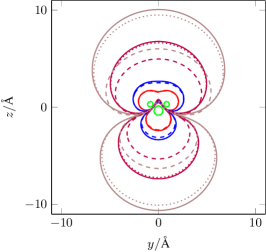
Figure 1: Absolute value of the electrostatic potential of a single SPC/E water molecule computed by Ewald summation (solid lines) and the Wolf method with $\zeta L=1.0$ (dotted lines) and $\zeta L=7.2$ (dashed lines). With increasing distance from the origin, the isolines of the potential correspond to the values $14.4~{}\text{V}$, $1.44~{}\text{V}$, $0.72~{}\text{V}$, $0.144~{}\text{V}$ and $0.072~{}\text{V}$, respectively.

It is obvious that for the strong damping (dashed lines) the potential decays too quickly as compared to the result we get with Ewald summation (solid lines). Only the short-range behaviour in the immediate vicinity of the molecule is captured correctly. The weaker damping parameter (dotted lines), on the other hand, yields a reasonable agreement with Ewald summation within a distance of about 6 Å from the origin, but shows some deviation further away. Employing even lower values for $\zeta$, for example $0.5/L$, reduces the discrepancy between the outermost contour lines only minimally (not shown). Since the value of the potential represented by the lowest contour level in Fig. 1 corresponds to only $0.5\%$ of the highest one, we conclude that the parameters $(\zeta L=1.0,r_{\text{c}}=L/2)$ yield a reasonable approximation to the Ewald result within the cutoff sphere of $11~{}\text{\AA}$. Validation of both sets of parameters in bulk simulations also reveals good agreement with Ewald summation (see Appendix B).

III Spatial averaging

Once the method to treat electrostatic interactions is chosen and optimised, one typically wishes to improve the statistics of the collected averages. For this purpose a simulation setup with high spatial symmetry is advantageous Armstrong and Bresme (2013). In this work, we focus on the case where the underlying three-dimensional problem can be reduced to one spatial dimension, as illustrated in Fig. 2. For such a system, the average charge density can only depend on $z$ for sufficiently long simulation times, because the system is isotropic in all other directions. Therefore, this approach is justified only if one considers sufficiently long simulations. Assuming $\rho_{q}(\mathbold r^{\prime})\equiv\rho_{q}(z^{\prime})$, we can then rewrite Eq. (2) as

$$\Phi(z)=\int\limits_{-L_{z}/2}^{L_{z}/2}\mathrm{d}z^{\prime}\ {G_{\text{1D}}}(z-z^{\prime})\rho_{q}(z^{\prime}),$$ (9)

where we introduced the one-dimensional kernel

$${G_{\text{1D}}}(z)=\int\limits_{-L_{x}/2}^{L_{x}/2}\mathrm{d}x^{\prime}\int\limits_{-L_{y}/2}^{L_{y}/2}\mathrm{d}y^{\prime}\ G(x-x^{\prime},y-y^{\prime},z).$$ (10)

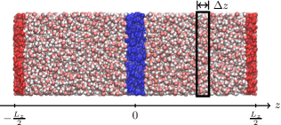
Figure 2: Simulation setup with a hot reservoir (coloured in red) wrapped around the boundaries and a cold reservoir (coloured in blue) in the centre of the simulation box. The superimposed rectangle (black solid lines) schematically illustrates a bin of width $\upDelta z$.

Taking the negative gradient of Eq. (9) yields the electrostatic field

$$E_{z}(z)=-\int\limits_{-L_{z}/2}^{L_{z}/2}\mathrm{d}z^{\prime}\ {G^{{}^{\prime}}_{\text{1D}}}(z-z^{\prime})\rho_{q}(z^{\prime}),$$ (11)

where $G_{\text{1D}}^{{}^{\prime}}$ denotes the derivative of $G_{\text{1D}}$. The above integrals can be evaluated readily for Ewald summation and the Wolf method (see Appendix A). The results can be improved considerably by averaging the potential and the microscopic field over small spatial regions, such that we obtain the macroscopic Maxwell field for the latter. The centre of each control volume then represents its exact spatial average. To this end, we consider $N_{\text{b}}$ bins of width $\upDelta z$, as depicted in Fig. 2. The lower and upper boundaries of bin $j$, where $j=1,\ldots,N_{\text{b}}$, are given by $z_{j,1}=-L_{z}/2+(j-1)\upDelta z$ and $z_{j,2}=z_{j,1}+\upDelta z$, respectively. The spatial average of the potential over bin $j$ is then given by

$${\bar{\Phi}}_{j} =\frac{1}{\upDelta z}\int\limits_{z_{j,1}}^{z_{j,2}}\mathrm{d}z\ \Phi(z)$$ (12a)

$$=\int\limits_{-L_{z}/2}^{L_{z}/2}\mathrm{d}z^{\prime}\ {{\bar{G}}_{\text{1D},j}}(z^{\prime})\rho_{q}(z^{\prime}),$$ (12b)

where the overbar denotes the spatially averaged kernel

$${\bar{G}}_{\text{1D},j}(z^{\prime})= \frac{1}{\upDelta z}\int\limits_{z_{j,1}}^{z_{j,2}}\mathrm{d}z\ {G_{\text{1D}}}(z-z^{\prime}).$$ (13)

For our effectively one-dimensional system of point charges, we can decompose the charge density according to

$$\rho_{q}(z)=\frac{1}{L_{x}L_{y}}\sum_{i}q_{i}\ \delta(z-z_{i}),$$ (14)

where $\delta(z)$ is the one-dimensional Dirac delta function. Inserting this expression back into our previous result for the potential yields

$${\bar{\Phi}}_{j} =\frac{1}{L_{x}L_{y}}\sum_{i}q_{i}\ {\bar{G}}_{\text{1D},j}(z_{i}).$$ (15)

Analogously, the averaged field is given by

$${\bar{E}}_{z,j} =-\frac{1}{L_{x}L_{y}}\sum_{i}q_{i}\ {\bar{G}}^{{}^{\prime}}_{\text{1D},j}(z_{i}).$$ (16)

The corresponding expressions for $\bar{G}_{\text{1D}}$ and ${\bar{G}}^{{}^{\prime}}_{\text{1D}}$ for Ewald summation are derived in Appendix A. The above averages for potential and field depend on all particle positions and therefore implicitly on time. The time average of any quantity $X$ is defined as

$$\langle{X}\rangle =\frac{1}{\tau}\int\limits_{0}^{\tau}\mathrm{d}t\ {X}(t),$$ (17)

where $\tau$ is the total simulation time of the production run. It is straightforward to evaluate $\langle{\bar{\Phi}}_{j}\rangle$ and $\langle{\bar{E}}_{z,j}\rangle$ for the discrete trajectory obtained from the NEMD simulation.

IV Multipole expansion

In what follows, we outline how the exact potential, as calculated from the charge density, can be decomposed into individual multipole contributions. This helps us to gain insight into how the alignment of the molecules with respect to the temperature gradient affects the field. We consider two different expansions for comparison which are illustrated in Fig. 3. In the slab expansion (Fig. 3a), the multipole moments due to the charges located inside a bin are calculated relative to its centre. In the molecule expansion (Fig. 3b), separate multipole expansions are carried out for each individual molecule and the multipoles are located at the respective oxygen sites. If all moments were considered in the expansion, both approaches would give rise to the same potential at a distant point $P$. We note that both types of expansion have already been considered in the past for interfacial systems Wilson, Pohorille, and Pratt (1989); Glosli and Philpott (1996). However, here we use a more general formulation Smith (1998) which is also applicable to modified kernels representing truncated Coulomb interactions.

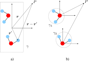
Figure 3: Illustration of two different multipole expansions: a) with respect to the centre of the region $\gamma$ (“slab expansion”) and b) for each molecule $\gamma_{j}$ individually with the oxygen site at the origin (“molecule expansion”). Both approaches give rise to the same field at a distant point $P$.

The potential generated by a charge distribution enclosed in a volume $\gamma$ is given by

$$\Phi(\mathbold r)=\int_{\gamma}\mathrm{d}^{3}r^{\prime}\ G(\mathbold r-\mathbold r^{\prime})\rho_{q}(\mathbold r^{\prime}).$$ (18)

From this equation we can obtain the contributions of the individual multipole moments by expanding $G(\mathbold r-\mathbold r^{\prime})$ into a Taylor series around $\mathbold r$,

$$\Phi(\mathbold r) \approx \phantom{{}-{}}G(\mathbold r)\underbrace{\int_{\gamma}\mathrm{d}^{3}r^{\prime}\rho_{q}(\mathbold r^{\prime})}_{q}$$ (19)

$$-\sum_{\alpha}\nabla_{\alpha}G(\mathbold r)\underbrace{\int_{\gamma}\mathrm{d}^{3}r^{\prime}r_{\alpha}^{\prime}\rho_{q}(\mathbold r^{\prime})}_{\mu_{\alpha}}$$

$$+\sum_{\alpha,\beta}\nabla_{\alpha}\nabla_{\beta}G(\mathbold r)\underbrace{\frac{1}{2}\int_{\gamma}\mathrm{d}^{3}r^{\prime}r_{\alpha}^{\prime}r_{\beta}^{\prime}\rho_{q}(\mathbold r^{\prime})}_{Q_{\alpha\beta}},$$

where $q$ is the total charge in $\gamma$, $\bm{\mu}$ the dipole moment and ${Q}$ the quadrupole moment. The symbol $\nabla_{\alpha}$ denotes the derivative with respect to the Cartesian component $r_{\alpha}$. Moving the origin of the charge distribution to $\tilde{\mathbold r}$ and taking into account the symmetry properties of our effectively one-dimensional system, we find

$$L_{x}L_{y}\Phi(z) \approx \phantom{{}+{}}\underbrace{{G_{\text{1D}}}(z-\tilde{z})\ q}_{\text{monopole contribution}}-\underbrace{G^{{}^{\prime}}_{\text{1D}}(z-\tilde{z})\ \mu_{z}}_{\text{dipole contribution}}$$ (20)

$$+\underbrace{G^{{}^{\prime\prime}}_{\text{1D}}(z-\tilde{z})\ {Q}_{zz}}_{\text{quadrupole contribution}}.$$

From the simulated trajectory, we then compute time averages of the multipole densities ${\bar{\rho}}_{q,j}$, ${\bar{\rho}}_{\mu,j}$ and ${\bar{\rho}}_{Q,j}$ for the monopole, dipole and quadrupole moments of every bin $j$, respectively. Before defining these quantities, we first introduce some additional notation to distinguish between the two types of expansion. We use superscripts $\cdot^{(m)}$, where $m=1$ for slabs (Fig. 3a) and $m=2$ for molecules (Fig. 3b). The density of $X=q,\mu_{z},Q_{zz}$ [cf. Eq. (19)] is then given by

$${\bar{\rho}}_{X,j}^{(1)}=\frac{1}{\upDelta v}\times\left\{\text{moment of bin $j$}\right\}$$ (21)

for the case $m=1$ and

$${\bar{\rho}}_{X,j}^{(2)}=\frac{1}{\upDelta v}\times\left\{\text{sum of molecular moments in bin $j$}\right\}$$ (22)

for the case $m=2$, where $\upDelta v=L_{x}L_{y}\upDelta z$ is the volume of the bin. Since we only consider the multipole moments $q$, $\mu_{z}$ and $Q_{zz}$, from now on we omit the subscripts for readability.

In general, the multipole moments depend on the way the charge distribution is partitioned Jackson (1998); Spaldin (2012) and consequently the multipole densities for slabs and molecules are not directly comparable. For example, the quadrupole moment of a reference bin will, in general, not be equal to the sum of the molecular quadrupole moments. Furthermore, we make an intentional, small mistake in the evaluation of ${\bar{\rho}}_{\mu,j}^{(2)}$ and ${\bar{\rho}}_{Q,j}^{(2)}$ for the sake of computational convenience, because we ignore the precise location of the molecular moments within the bin $j$. However, as we will see in Sec. VI, the error in the electrostatic potential introduced by this approximation is negligible.

The electrostatic potential (at the centre of bin $j$) is then calculated as the sum of the three contributions in Eq. (20),

$$\Phi^{(m)}_{j}=\Phi^{(m)}_{q,j}+\Phi^{(m)}_{\mu,j}+\Phi^{(m)}_{Q,j},$$ (23)

which are given by

$$\Phi^{(m)}_{q,j} = \phantom{{}-{}}\upDelta z\sum_{l=1}^{N_{\text{b}}}{G_{\text{1D}}}(z_{j}-z_{l}){\bar{\rho}}_{q,l}^{(m)},$$ (24a)

$$\Phi^{(m)}_{\mu,j} = -\upDelta z\sum_{l=1}^{N_{\text{b}}}G_{\text{1D}}^{{}^{\prime}}(z_{j}-z_{l}){\bar{\rho}}_{\mu,l}^{(m)},$$ (24b)

$$\Phi^{(m)}_{Q,j} = \phantom{{}-{}}\upDelta z\sum_{l=1}^{N_{\text{b}}}G_{\text{1D}}^{{}^{\prime\prime}}(z_{j}-z_{l}){\bar{\rho}}_{Q,l}^{(m)},$$ (24c)

respectively. Since the molecules are charge-neutral, it follows that all values $\rho_{q,j}^{(2)}$ and consequently $\Phi_{q,j}^{(2)}$ vanish identically.

V Simulation protocol

For production runs, we prepared the system in the same state as Armstrong and Bresme Armstrong and Bresme (2013) in order to carry out a quantitative comparison. The simulation box (Fig. 2) has exactly the same dimensions as the one used for the model system. For two of the three NEMD simulations we used the Wolf method and the remaining one was performed with Ewald summation (the relevant parameters are summarised in Sec. II.3). Lennard-Jones interactions were truncated at $11~{}\text{\AA}$ in all cases. The box contains $N=4500$ SPC/E molecules resulting in a mass density of $\rho_{m}=0.934~{}\text{g}/\text{cm}^{3}$. All simulations were carried out using a modified version of the software package LAMMPS (9Dec14) Plimpton (1995) which we augmented with the eHEX/a algorithm Wirnsberger, Frenkel, and Dellago (2015).

V.1 Equilibration

The system was first equilibrated and validated. Starting from an initial lattice structure with zero linear momentum, we integrated the equations of motion with the velocity Verlet algorithm Swope et al. (1982) employing a timestep of ${\upDelta t=1~{}\text{fs}}$. For the first $20$ ps we rescaled the velocities to drive the system close to the target temperature of $400~{}\text{K}$. This was followed by a short 200 ps NpT run using a Nosé–Hoover thermostat with a relaxation time of $\tau_{T}=1~{}\text{ps}$ and a Nosé–Hoover barostat with a relaxation time of $\tau_{p}=2.5~{}\text{ps}$ Nosé (1984); Hoover (1985). We then rescaled the box to the target dimensions and carried out a $500$ ps NVT run during which we monitored the average system energy. Next, we adjusted the kinetic energy of the last configuration by velocity rescaling and used it as input for another $1$ ns NVE equilibration run. The average temperature during this run was $T=(400\pm 0.1)~{}\text{K}$, where the error bar was estimated using block average analysis Frenkel and Smit (2002). We computed the pair-correlation function, the velocity autocorrelation function, the dielectric constant and the distance-dependent Kirkwood $g$-factor (see Appendix B). The validation suggests that our implementation is correct and our choice of parameters reasonable.

V.2 Non-equilibrium stationary state

To investigate the effect of a thermal gradient after the equilibration, the system was driven to a non-equilibrium stationary state by imposing a constant heat flux between two reservoirs, $\Gamma_{1}$ and $\Gamma_{2}$ (Fig. 2). This was achieved by introducing an additional force, $\mathbold g_{i}$, to the equations of motion Wirnsberger, Frenkel, and Dellago (2015), such that

$$\dot{\mathbold r}_{i} =\mathbold v_{i},$$ (25a)

$$\dot{\mathbold v}_{i} =\frac{\mathbold f_{i}}{m_{i}}+\frac{\mathbold g_{i}}{m_{i}},$$ (25b)

where $m_{i}$ is the mass of atom $i$ and $\mathbold f_{i}$ the force calculated from the potential. The thermostatting force is defined as

$$\mathbold g_{i}=\begin{cases}m_{i}\frac{\mathcal{F}_{\Gamma_{k(\mathbold r_{i})}}}{2\mathcal{K}_{\Gamma_{k(\mathbold r_{i})}}}\left(\mathbold v_{i}-\mathbold v_{\Gamma_{k(\mathbold r_{i})}}\right)&\mbox{if $k(\mathbold r_{i})>0$,}\\ 0&\mbox{otherwise, }\end{cases}$$ (26)

where $k(\mathbold r_{i})\in\{0,1,2\}$ is an indicator function which maps the particle to the region $\Gamma_{k}$ in which it is located and $\mathcal{F}_{\Gamma_{k}}$ is a constant energy flux into $\Gamma_{k}$. Those parts of the simulation box which are not thermostatted are labelled with $\Gamma_{0}$. The non-translational kinetic energy of the region $\Gamma_{k}$ is given by

$${\mathcal{K}}_{\Gamma_{k}}=\sum_{{i\in\gamma_{k}}}\frac{m_{i}v_{i}^{2}}{2}-\frac{m_{\Gamma_{k}}v_{\Gamma_{k}}^{2}}{2},$$ (27)

where the quantities $\mathbold v_{\Gamma_{k}}$ and $m_{\Gamma_{k}}$ are the centre of mass velocity and the total mass of $\Gamma_{k}$, respectively, and the index set $\gamma_{k}$ comprises all particles which are located inside that region Wirnsberger, Frenkel, and Dellago (2015).

The equations were solved numerically with our recently proposed eHEX/a algorithm Wirnsberger, Frenkel, and Dellago (2015) with a timestep of $\upDelta t=2~{}\text{fs}$. For the symmetric setup shown in Fig. 2, the heat flux is trivially related to the energy flow into the reservoir by

$$J_{Q,z}=\frac{F_{\Gamma_{1}}}{2L_{x}L_{y}},$$ (28)

where the factor of 2 in the denominator accounts for the periodic setup. After switching on the thermostat, we waited for 10 ns for any transient behaviour to disappear before starting with the $\tau=60~{}\text{ns}$ production run. The energy conservation was excellent ($|\upDelta E/E|\approx 0.005\%$) and the centre of mass velocity of the simulation box remained close to machine precision throughout the simulation. The heat fluxes are input parameters of the eHEX algorithm which were adjusted by trial and error. The employed values are summarised in Tab. 1.

Table 1: Imposed heat fluxes and measured values for the tempature gradients. We note that our heat flux for the Wolf ($\zeta L=7.2$) run is about 1.7% larger than the value used by Armstrong and Bresme Armstrong and Bresme (2013).

	$J_{Q,z}$ ($10^{10}~{}\text{W}/{\text{m}^{2}}$)	$\nabla T$ (K/Å)
Ewald	4.243	$-5.14\pm 0.04$
Wolf ($\zeta L=1.0$)	4.166	$-5.17\pm 0.04$
Wolf ($\zeta L=7.2$)	3.875	$-5.18\pm 0.04$

We note that lower heat fluxes are required for the Wolf method in order to achieve the same temperature gradient as for Ewald summation. This is consistent with the observation that the truncation of electrostatic interactions results in lower thermal conductivities Muscatello and Bresme (2011).

VI Results

In this section, we present the key results for the temperature and density profiles (Sec. VI.1), the multipole expansions (Sec. VI.2), the potential (Sec. VI.3), the field (Sec. VI.4) and the polarisation (Sec. VI.5). We estimated error bars for all results in this section. To this end we divided the entire trajectory into 600 blocks (of length $100~{}\text{ps}$) and assumed the results for the individual blocks to be uncorrelated. The size of the individual error bar then corresponds to twice the standard deviation of the mean. This estimate comprises the statistical error as well as the methodological error arising, for example, from the employed quadrature.

VI.1 Temperature and density

Figures 4a-b show the spatial variations in temperature and density along the $z$-direction with a resolution of $\upDelta z=2.73~{}\text{\AA}$ ($N_{\text{b}}=40$).

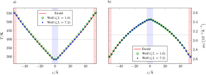
Figure 4: Spatial variation of a) temperature and b) oxygen number density obtained with Ewald summation and the Wolf method. The horizontal lines indicate the spatial and temporal equilibrium averages of the temperature and the number density, respectively. The vertical stripes indicate the locations of the hot (coloured in red) and cold (coloured in blue) reservoirs.

The temperature of an individual bin was calculated from the non-translational kinetic energy of the atoms inside that bin Wirnsberger, Frenkel, and Dellago (2015). There are only small differences between the results obtained with the Ewald and Wolf methods. The peak temperature at the centre of the hot reservoir is about $552~{}\text{K}$ and the lowest temperature at the centre of the cold reservoir is about $285~{}\text{K}$ (Fig. 4a). The temperature profile is linear outside the reservoirs and symmetric with respect to the origin of the simulation box, which is in accordance with the setup.

The measured average number densities (Fig. 4b) obtained with Ewald summation and the Wolf method agree well apart from slight differences in the vicinity of the cold reservoir. The mass density varies by up to 15% (cold reservoir) with respect to $\rho_{m}$. We note that on this scale, we did not observe any appreciable discontinuities of the temperature or density close to the reservoir boundaries, although the thermostatting force is discontinuous.

VI.2 Molecular orientation and multipole moments

In this section, we discuss the induced molecular alignment and multipole moments due to the thermal gradient for both expansions in Fig. 3. The left column in Fig. 5 corresponds to the slab (centre-of-bin) expansion and the right column to the molecule expansion. The monopole in the molecule expansion vanishes identically, hence it is not shown. The spatial variations of all quantities are shown with a resolution of $\upDelta z=5.45~{}\text{\AA}$ ($N_{\text{b}}=20$).

Let us consider the time averaged charge density for slabs first (Fig. 5a). For Ewald summation the error of the average is so large that it swamps the signal even after 60 ns of simulation time. We also note that the curve is not symmetric in the vicinity of the cold reservoir within the statistical uncertainty shown in the plot. We believe that this may be due to the fact that we computed the error bars as if neighbouring bins were independent, which is not the case, because molecules are charge neutral. The real error bars may be larger due to long-wavelength fluctuations. We confirmed that the results become symmetric (within the statistical error) upon doubling the simulation time.

For the Wolf method there is an accumulation of positive charge in the vicinity of the hot reservoir, which is enhanced by stronger damping. This result agrees qualitatively with the findings of Rodgers and Weeks for a different inhomogeneous system, where the authors compared the (Gaussian-smoothed) charge density obtained with Gaussian-truncated (GT) water to that of Ewald summation Rodgers and Weeks (2008a). Furthermore, we note that the error bar increases by about one order of magnitude upon refining the resolution by a factor of 10, which corresponds to $\upDelta z\approx 0.54~{}\text{\AA}$ ($N_{\text{b}}=200$) used by Armstrong and Bresme Armstrong and Bresme (2013).

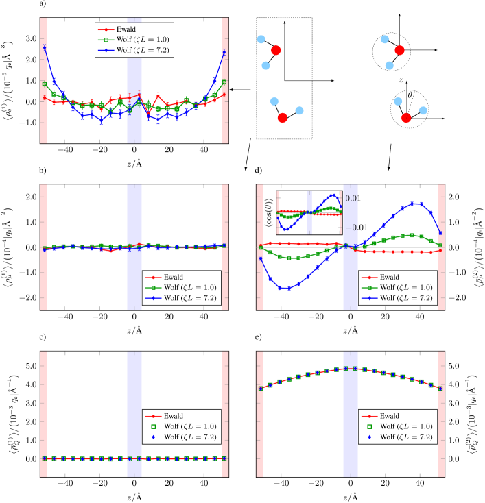
Figure 5: Multipole densities for the slab expansion (left column) and molecule expansion (right column). The panels a-c) show the charge density, dipole density and quadrupole density, respectively, for the slab expansion. The panels d) and e) show the dipole density and quadrupole density, respectively, for the molecule expansion. The inset in panel d) shows the average molecular alignment with the temperature gradient. Horizontal lines in the inset and the full figure were added to highlight the symmetry of the result.

Figures 5b and d show the dipole densities for both expansions, respectively. For the slabs (Fig. 5b), there is no noticable trend of the dipole density within the statistical uncertainity. However, for the molecule expansion (Fig. 5d) we find a strong disagreement between the two electrostatic kernels. For this case, we also quantified the average molecular alignment using the order parameter Römer et al. (2012)

$$\cos(\theta)=\mathbold n\cdot\mathbold e_{z},$$ (29)

where $\mathbold n=\mathbold\mu/\mu$ defines the orientation of a molecule and $\mathbold e_{z}$ is the unit vector in the direction of the temperature gradient. In the case of Ewald summation molecules, on average, point to the cold reservoir and the alignment is fairly constant outside the reservoirs (see inset in Fig. 5d). The Wolf method entirely fails to capture this behaviour. For the wide range of parameters considered in this work (including the ones previously employed in the literature), the method predicts opposite orientations and overestimates the magnitude of alignment by a factor of about 7 for the strong damping. Employing a lower value for the damping parameter reduces the overestimation, but cannot correct the wrong sign. We also note that our results for the average molecular orientation (inset in Fig. 5d) are in agreement with the ones reported by Armstrong and Bresme Armstrong and Bresme (2013).

The quadrupole densities, shown in Figs 5c and e, agree well with each other within each expansion. Similarily to the dipole density, considering slabs for the expansion (Fig. 5c) yields results which are negligible compared to the molecule expansion (Fig. 5e). We note that in the latter case, the profile is proportional to the oxygen number density (Fig. 4b) and can lead to considerable contributions to the potential.

Repeating our simulation with Ewald summation and vacuum boundary conditions (see Refs Hummer et al., 1999; De Leeuw, Perram, and Smith, 1980 for more details), we found consistent results for the multipole densities (not shown). We can therefore rule out any artifacts arising from the boundary conditions at infinity on the results shown in this section. However, we noticed that the statistical error of the molecular dipole density decays much faster for vacuum boundary conditions relative to tin-foil boundary conditions.

VI.3 Electrostatic potential

In the previous section, we analysed the thermally induced multipole moments for two different multipole expansions, namely slabs and molecules. The aim of this section is to compare three different ways of calculating the electrostatic potential: Firstly, we consider the exact analytical average given by Eq. (15). Secondly, we approximate the potential using only the average charge density given by the slab expansion, Eq. (24a), which is the approach regularly employed in the literature Wick, Dang, and Jungwirth (2006); Wilson, Pohorille, and Pratt (1988); Yeh and Berkowitz (1999); Armstrong and Bresme (2013). Thirdly, we approximate the potential using also the dipole and quadrupole densities, i.e. Eqs (24b-c).

Let us consider the results for the exact calculation first, which are shown in Fig. 6a. All graphs are symmetric with respect to the origin of the simulation box and periodic, indicating that the field vanishes at the centres of the reservoirs. Although the shape of the potential predicted by the short-ranged method is similar to the one for Ewald summation, the results are sensitive to the choice of damping parameter. Weak damping overestimates the potential, whereas strong damping leads to an underestimation. Both our choices fail to reproduce the Ewald summation result correctly, although it seems plausible that intermediate values for the damping parameter could lead to a better agreement.

Figure 6b compares (for Ewald summation) the exact result for the electrostatic potential to that given by the monopole density in the slab expansion. We recall that the latter approach corresponds to averaging the charge density first and integrating it with the appropriate kernel afterwards [Eq. (24)a]. It is clear from comparison of the two curves including error bars that the exact calculation yields a huge improvement over the approximation. For the resolution shown in the plot ($N_{\text{b}}=40$, $\upDelta z=2.73~{}\text{\AA}$), the error bars are reduced by more than one order of magnitude. The inset shows the ratio of the maximum error of the approximation to the maximum error of the exact calculation as a function of the number of bins. (We define the maximum error to be half the length of the largest error bar throughout the entire interval.) For a very low resolution of 10 grid points ($\upDelta z=10.9~{}\text{\AA}$), the maximum error decreases by about a factor of 26. For high resolutions of $\upDelta z\leq 0.5~{}\text{\AA}$ the error ratio approaches unity implying that both methods become comparable, which is the expected behaviour in the limit $\upDelta z\to 0$. At the same time the magnitude of the error naturally increases for higher resolutions because fewer molecules contribute to a particular bin (for 400 bins the maximum error increases by about $50\%$ as compared to the resolution of 40 bins shown in the figure).

Given that molecules point, on average, in opposite directions for the two electrostatic kernels (Fig. 5d), it is counterintuitive that the potentials are qualitatively comparable. To understand the origin of this seeming contradiction, we singled out the individual multipole contributions, which are illustrated in Figs 7a-d for both expansions. Let us consider the slab expansion first. For both electrostatic kernels (Figs 7a-b) we found the monopole contribution (black curve) to capture the exact potential (red line) reasonably well for the chosen spatial resolution ($N_{\text{b}}=40$, $\upDelta z=2.73~{}\text{\AA}$). However, if we consider a point dipole and a point quadrupole (representative for the respective bin average) in addition to the point monopole located at the centre of each bin, we obtain a much better approximation to the exact result (red circles). In fact, for Ewald summation we recover the exact potential almost perfectly, whereas we observe an overshoot inside the hot reservoir for the Wolf method. We believe that a more accurate approximation for the short-ranged method might be obtained by considering octupole and hexadecapole contributions in addition, but we did not investigate this further.

The situation changes entirely for the molecule expansion shown in Figs 7c-d, where the monopole contribution is zero. For Ewald summation (Fig. 7c), the dipole density leads to a linear potential outside the reservoirs (green curve) corresponding to a negative field in the left half of the simulation box. However, close to the hot reservoir the quadrupole contribution (blue curve) outweighs the dipole contribution causing the slope of the overall potential to be negative and therefore the field to be positive. In the vicinity of the cold reservoir the dipole contribution dominates over the quadrupole contribution and the field is negative. The sum of both terms (red circles) agrees perfectly with the exact average (red line). For the Wolf method we found that the quadrupole density constitutes a much smaller correction to the dipole contribution which is almost negligible outside the reservoirs. This might seem surprising at first given that the results for the quadrupole densities agree well for both summation methods (Fig. 5e). The apparent contradiction is explained by the fact that the derivatives of the kernels in the evaluation of the potential are very different for both methods. We will get back to this point in Sec. VI.5 when we discuss the macroscopic polarisation.

With regard to the accuracy of the full multipole approximations (up to the quadrupole term), we observed different trends for the maximum error of the potential within each expansion. For the slab expansion we found the maximum error to be about 6 times larger than the error of the exact potential for the lowest resolution ($N_{\text{b}}=10$, $\upDelta z=10.9~{}\text{\AA}$). Upon increasing the resolution, the error ratio approaches unity, which is the expected behaviour. However, this is not the case for the molecule expansion, where the error is only about $20\%$ larger than the error of the exact potential initially, but the difference increases to about $100\%$ for the highest resolution ($N_{\text{b}}=3200$, $\upDelta z=0.034~{}\text{\AA}$). We believe that this behaviour is reasonable, because we never intersect molecules and cannot resolve the potential inside a molecule correctly. The higher the resolution the worse we expect the approximation to become in the vicinity of the point multipoles. Averaging the potential exactly is preferable on all scales, rendering it clearly the method of choice.

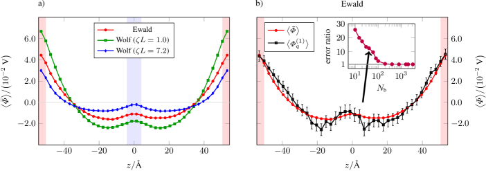
Figure 6: The exact potential is shown in panel a) and a comparison between the potential calculated solely from the monopole density in the slab expansion and the exact result calculated with Ewald summation is shown in b). The inset compares the ratio of the maximum errors which were calculated from 600 blocks of length $100~{}\text{ps}$ as a function of the number of bins. The arrow indicates the error ratio for the resolution shown in the full figure.

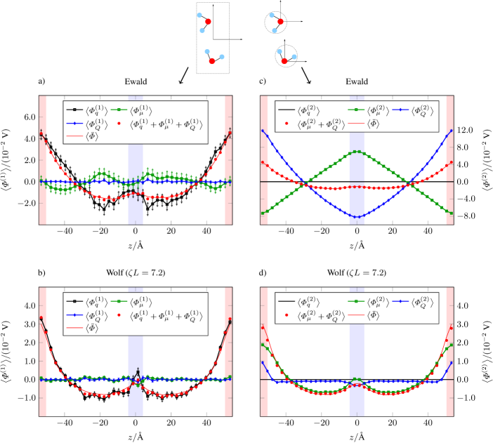
Figure 7: Individual contributions to the potential for the slab expansion (left column) and molecule expansion (right column). The results for Ewald summation are shown in panels a) and c) in the first row and for the Wolf method in panels b) and d) in the second row.

VI.4 Electrostatic field

The exact results for the field in the sense of Eq. (16) are shown in Fig. 8a. Focusing on the left half of the simulation box, we notice that the field is positive and strongest in the vicinity of the hot reservoir. For the peak field strength we measured values of about $2.8\times 10^{7}~{}\text{V/m}$, $4.4\times 10^{7}~{}\text{V/m}$ and $2.2\times 10^{7}~{}\text{V/m}$ for Ewald summation and the Wolf method with weak and strong damping, respectively. Close to the hot reservoir, the short-ranged method overshoots the Ewald summation result for low damping and vice versa for high damping. We also infer from the figure that the field changes its sign in the vicinity of the cold reservoir. From the discussion of the potentials in the previous section (Fig. 7c) we know that the inversion happens exactly when the dipole contribution to the field dominates over the quadrupole contribution.

Comparing our results to the ones reported by Bresme and co-workers, we find a major discrepancy: In the original work Armstrong and Bresme (2013) the reported fields are about one order of magnitude higher than what we found. Recently, however, it was suggested that the thermally induced field in a spherical droplet of SPC/E water is of the order of $10^{7}~{}\text{V/m}$ after comparison with Ewald summation (PPPM) Armstrong, Daub, and Bresme (2015). Nevertheless, the discrepancy still persists as the authors Armstrong, Daub, and Bresme (2015) suggest that the Wolf method itself is responsible for the overestimated field, whereas, in fact, the opposite is true for the set of parameters employed in Ref. Armstrong and Bresme, 2013. The Wolf method slightly underestimates the field if it is calculated consistently, namely using the correct kernel (see Fig. 8a). We can reproduce the results of Armstrong and Bresme closely if we calculate the field as Armstrong and Bresme (2013)

$$E_{z}(z)=4\pi\int\limits_{-L_{z}/2}^{z}\mathrm{d}z^{\prime}\rho_{q}(z^{\prime}),$$ (30)

considering Gaussian units and taking the lower integration bound to be $-L_{z}/2$ rather than $-\infty$. (A comparison is omitted for brevity.) For Ewald summation this expression is correct and equivalent to Eq. (11) with $G^{{}^{\prime}}_{\text{1D,E}}$ as long as the net dipole density of the box,

$$\bar{\rho}_{\mu,L_{z}}=\frac{1}{L_{z}}\int\limits_{-L_{z}/2}^{L_{z}/2}\mathrm{d}z^{\prime}z^{\prime}\rho_{q}(z^{\prime}),$$ (31)

vanishes. Considering sufficiently long simulations, this is necessarily the case for our system because of the symmetric setup (see Figs 2, 5b and d). If this was not the case, an additional term $4\pi\bar{\rho}_{\mu,L_{z}}$ would have to be added to the right-hand side of Eq. (30). The equivalence is trivially shown by rewriting the integral in Eq. (11) taking into account periodicity and charge neutrality. Alternatively, one can integrate Poisson’s equation directly and impose periodicity by choosing the integration constants accordingly Yeh and Wallqvist (2011). However, applying Eq. (30) for the Wolf method is wrong and the discrepancy between our result and the one of Armstrong and Bresme Armstrong and Bresme (2013) can therefore be traced back to using the incorrect expression in the calculation.

Similarly to what we observed for the potential, considering exact averages rather than estimating the field from the average charge density yields a huge improvement for low resolutions. The comparison in Fig. 8b is carried out for a resolution of $N_{\text{b}}=10$ ($\upDelta z=10.9~{}\text{\AA}$) and, as shown in the inset, the error of the approximative field, i.e. using the negative derivative of $G_{\text{1D,E}}$ in Eq. (24a), is about 10 times larger than the exact one. For resolutions higher than $N_{\text{b}}=80~{}\text{bins}$ ($\upDelta z\leq 1.36~{}\text{\AA})$, both approaches yield similar errors. Comparing the insets of Figs 6b and 8b, we notice that the enhancement of the exact method over the approximative one is much higher for the potential. This can be partly explained by looking at the functional form of $G^{{}^{\prime}}_{\text{1D,E}}$ (Eq. (44a) in Appendix A). The function is piecewise linear and the midpoint rule, which corresponds to multiplying the function value at the centre of the bin by $\upDelta z$, is exact in the absence of any discontinuity. Therefore, the advantage of using ${\bar{G}}^{{}^{\prime}}_{\text{1D,E}}$ over ${G}^{{}^{\prime}}_{\text{1D,E}}$ for the evaluation of the field is less significant than for the potential.

Figure 9 compares the spatial maximum errors for varying resolutions. Interestingly, for sufficiently high resolutions of $\upDelta z\leq 1~{}\text{\AA}$ we found the maximum error of the approximative method to be up to almost 30% lower than the one for the exact average. We attribute this to cancellation of errors, since convergence tests support a correct implementation. Far more important is the magnitude of the error for high resolutions. For simulation time scales of $100~{}\text{ns}$ the error is comparable to the signal itself requiring even longer runs for the statistics to be satisfactory. Suppose we wanted to get a rough idea of what the field looked like. With the conventional method, i.e. averaging the charge density first and then integrating it, the best we can do is to calculate the results on a sufficiently high resolution and then perform some sort of averaging. On the one hand, this approach is problematic because the coarse-grained values do not represent the correct bin averages. On the other hand, it is not straightforward to propagate the statistical errors from the fine resolution to the coarse one since the values are highly correlated. Our proposed method of averaging the potential and the field analytically eliminates both issues and yields a huge improvement for low resolutions reducing the required simulation time scales by up to two orders of magnitude for the same quality of statistics.

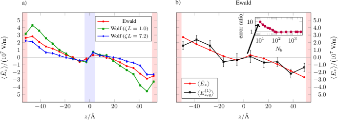
Figure 8: The exact field is shown in figure a) and a comparison between the field calculated from the monopole density in the slab expansion and the exact result is shown in b). The inset compares the ratio of the maximum errors which were calculated from 600 blocks of length $100~{}\text{ps}$ as a function of the number of bins. The arrow indicates the error ratio for the resolution shown in the full figure.

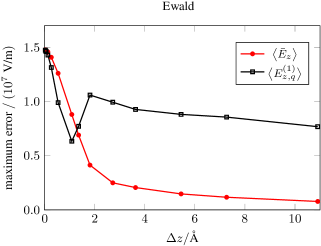
Figure 9: Spatial maximum error as a function of the resolution $\upDelta z$ for the exact field (red circles) and the monopole field (black, open squares), respectively. (The error is defined as one standard deviation of the mean and the error bar in Fig. 8b corresponds to twice the value for $\upDelta z=10.9~{}\text{\AA}$.)

VI.5 Macroscopic polarisation

Our final goal in this section is to relate the molecular multipole densities to the macroscopic polarisation. We show that the macroscopic Maxwell equation

$${\bar{E}}_{z}(z)={\bar{D}}_{z}(z)-4\pi{\bar{P}}_{z}(z)$$ (32)

holds locally for the bin averages calculated with Ewald summation, where ${\bar{P}}_{z}$ and ${\bar{D}}_{z}$ are the $z$-components of polarisation and displacement field, respectively. We do not make any a priori assumptions about the locality Neumann (1986a) and use the multipole expansions developed in Sec. IV as a general starting point for the discussion. We then identify the quantities on the right-hand side of Eq. (32) after simplifying the expressions. We note that our analysis only holds in the context of sufficiently long simulations (like in Sec. IV), because we use $\rho_{q}(z)$ in place of the full $\rho_{q}(\mathbold r)$. This simplifies the discussion in that we only need to consider the $z$-component of the spatially averaged dipole density, $\bar{\rho}_{\mu}$, and the density of $Q_{zz}$ given by $\bar{\rho}_{Q}$, respectively.

The water molecules comprise the polarisable background medium and there are no free charges. From our discusion in Sec. VI.3, we know that the dipole contribution alone yields a poor approximation to the potential (Figs 7c and d). As a natural extension we considered the quadrupole contribution Böttcher (1973), which was also found to be important in simulation studies of interfacial electric fields Wilson, Pohorille, and Pratt (1989); Glosli and Philpott (1996); Sokhan and Tildesley (1997). With the inclusion of this contribution, the potentials from the molecular multipole expansions match the exact potentials very well for both methods, respectively. The corresponding expression for the field extends to

$${\bar{E}}_{z}(z) = \int\limits_{-\frac{L_{z}}{2}}^{\frac{L_{z}}{2}}\mathrm{d}z^{\prime}\ \bigg{[}G_{\text{1D}}^{{}^{\prime\prime}}(z-z^{\prime}){\bar{\rho}}_{\mu}(z^{\prime})-G_{\text{1D}}^{{}^{\prime\prime\prime}}(z-z^{\prime}){\bar{\rho}}_{Q}(z^{\prime})\bigg{]}$$ (33a)

$$= \int\limits_{-\frac{L_{z}}{2}}^{\frac{L_{z}}{2}}\mathrm{d}z^{\prime}\ G_{\text{1D}}^{{}^{\prime\prime}}(z-z^{\prime})\left[{\bar{\rho}}_{\mu}(z^{\prime})-{\bar{\rho}}^{{}^{\prime}}_{Q}(z^{\prime})\right],$$ (33b)

where the derivatives of the kernels are given in Appendix A. To get to Eq. (33b) we integrated the second term in Eq. (33a) by parts taking into account the periodicity. We can solve the above integral analytically for Ewald summation and find that

$${\bar{E}}_{z}(z)=-4\pi\left[{\bar{\rho}}_{\mu}(z)-{\bar{\rho}}_{\mu,L_{z}}-{\bar{\rho}}^{{}^{\prime}}_{Q}(z)\right],$$ (34)

where ${\bar{\rho}}_{\mu,L_{z}}$ is the box average of ${\bar{\rho}}_{\mu}(z)$. In general, we can identify this contribution with ${\bar{D}}_{z}$ as it corresponds to the (constant) field arising from an induced surface charge density at infinity (tin-foil boundary conditions). We refer to Refs Stengel, Spaldin, and Vanderbilt, 2008 and Zhang and Sprik, 2016 for a more general discussion. Although the instantaneous value of ${\bar{D}}_{z}$ may fluctuate, we know that its time average vanishes, because our system does not exhibit a net dipole moment (Figs 5b and d). For Ewald summation the definition of polarisation as

$${\bar{P}}_{z}(z)={\bar{\rho}}_{\mu}(z)-{\bar{\rho}}^{{}^{\prime}}_{Q}(z)$$ (35)

therefore naturally leads to the correct proportionality of $\langle{\bar{P}}_{z}(z)\rangle=-\langle{\bar{E}}_{z}(z)\rangle/4\pi$. For the Wolf method the relation between electric field and polarisation (as defined above) is more complicated, because we cannot solve the integral in Eq. (33b) analytically. More importantly, we cannot expect the short-ranged method to predict fields accurately in general, because its kernel is not a solution of Poisson’s equation. The estimates for the thermally induced fields might be reasonable, but it is trivial to come up with an example, such as a plate capacitor, for which the method would fail.

Finally, we would like to discuss the macroscopic Maxwell equation (32) in the context of the slab expansion. As shown in Figs 7a-b, we can identify all relevant multipole contributions to the potential and recover a good approximation to the exact solution implying overall consistency. Due to the nature of the spatial averaging, we obtain a non-vanishing charge density (Fig. 5a) for our inhomogeneous system. This is inconsistent, however, with the derivation of Eq. (32), where charges within a molecule are summed first in order to get from the microscopic to the macroscopic description Jackson (1998); Böttcher (1973) and the charge density vanishes identically. Identification of displacement field and polarisation is therefore not meaningful for the slab expansion. This problem is avoided altogether in the molecule expansion, which is consistent with Eq. (32), and we can unambiguously identify all terms in the macroscopic Maxwell equation.

VII Conclusions

In this paper we have analysed the electric fields and multipole moments induced by a strong thermal gradient in NEMD simulations of water in a setup which was previously studied by Armstrong and Bresme Armstrong and Bresme (2013). Our comparison comprises results for two different treatments of Coulomb interactions, namely Ewald summation and the short-ranged Wolf method. The latter was employed in most of the previous studies on the thermo-polarisation effect Bresme et al. (2008); Muscatello et al. (2011); Armstrong and Bresme (2013); Armstrong, Lervik, and Bresme (2013); Armstrong, Daub, and Bresme (2015). We identified two key differences to the literature data: Firstly, the Wolf method fails to reproduce the dipole density correctly for parameters that work well in equilibrium simulations. The molecules point, on average, in opposite directions as compared to Ewald summation and the alignment is strongly enhanced.

Secondly, for both methods the peak field strength is of the order of $10^{7}~{}\text{V/m}$. However, for the Wolf method the result depends sensitively on the employed parameters. For low damping the Wolf method slightly overestimates the field obtained with Ewald summation and vice versa for high damping. The results are therefore in direct constrast to very recent findings of Bresme and co-workers Armstrong, Daub, and Bresme (2015) who reported that the Wolf method overestimates the field by an order of magnitude. In fact, we argue that the employed formula for the calculation of the field is incorrect. Taking such truncation into account correctly results in comparable results for the electric field.

Another key result of this paper are the highly improved spatial averages of the potential and the field for low resolutions. We propose to integrate these quantities analytically over the bins rather than calculating them from the time-averaged charge density, as is usually done in the literature. Potentials and fields then truly represent the exact spatial averages over the microscopic or macroscopic control volumes. We showed that this procedure is straightforward for both summation methods and requires no computational overhead. Comparing the ratio of maximum errors, we found a more than 20-fold reduction of the error for the potential and a 10-fold reduction for the field at the coarsest resolution of $\upDelta z\approx 10.9~{}\text{\AA}$. Consequently, employing the new method can reduce the simulation time scales by up to two orders of magnitude for the same quality of statistics. The advantage of calculating analytical averages becomes less significant with increasing spatial resolution and both methods are comparable for resolutions of $\upDelta z\leq 1~{}\text{\AA}$. However, in this case the magnitude of the statistical error is comparable to the signal itself rendering the results meaningless.

In addition, we found that accurate estimates of the potential and the field can be obtained by approximating the water molecules as ideal point dipoles and quadrupoles. For low spatial resolutions we found this approach to yield considerably better results than the calculation from the averaged charge density. Our detailed comparison of the results for the slab and molecule expansions illustrates that the ratio of the individual contributions depends on the control volume we choose for the expansion. For slabs almost all the information can be recovered by considering the monopole, as is usually done in the literature. However, in the molecule expansion the dipole and the quadrupole contributions are significant and both have to be considered in order to recover results from the exact calculation accurately.

Finally, taking into account the quadrupole contribution leads to the expected proportionality between the polarisation and the macroscopic Maxwell field in accordance with the macroscopic Maxwell equations. The Wolf method fails to satisfy this relation entirely. Based on its shortcomings, we therefore conclude that the method is not suitable for reproducing the electrostatic key quantities in inhomogeneous systems reliably. This is in agreement with the findings of Takahashi and co-workers Takahashi, Narumi, and Yasuoka (2011), who reported poor predictions for the electrostatic potential and dipolar orientations in simulations of the liquid–vapour interface, even for cutoff radii almost six times larger than the maximum value considered in this work.

Appendix A Electrostatics

A.1 Wolf method

Our goal is to integrate $G_{\text{W}}$ over the entire cutoff sphere in order to obtain ${G}_{\text{1D,W}}$. To this end we have to evaluate the integral

$${G}_{\text{1D,W}}(z) =\int\limits_{-\frac{L_{x}}{2}}^{\frac{L_{x}}{2}}\mathrm{d}x\ \int\limits_{-\frac{L_{y}}{2}}^{\frac{L_{y}}{2}}\mathrm{d}y\ G_{\text{W}}(x,y,z)$$ (36a)

$$=2\pi\int\limits_{0}^{s_{\text{c}}(z)}\mathrm{d}s\ s\left[\frac{\text{erfc}(\zeta\sqrt{s^{2}+z^{2}})}{\sqrt{s^{2}+z^{2}}}-\frac{\text{erfc}(\zeta r_{\text{c}})}{r_{\text{c}}}\right],$$ (36b)

where $r^{2}=x^{2}+y^{2}+z^{2}=s^{2}+z^{2}$. We first consider the integral

$$I(z)=\int\limits_{0}^{s_{\text{c}}(z)}\mathrm{d}s\ s\frac{\operatorname{erfc}(\zeta\sqrt{s^{2}+z^{2}})}{\sqrt{s^{2}+z^{2}}}$$ (37)

and use the substitution $\tau(s,z)=\sqrt{s^{2}+z^{2}}$ to rewrite the expression as

$$I(z)=\int\limits_{\tau(0,z)}^{\tau(s_{\text{c}}(z),z)}\mathrm{d}\tau\ \operatorname{erfc}(\zeta\tau).$$ (38)

Using integration by parts it is easy to show that the result is

$$I(z)=r_{\text{c}}\operatorname{erfc}(\zeta r_{\text{c}})-|z|\operatorname{erfc}(\zeta|z|)+\frac{\text{e}^{-\zeta^{2}z^{2}}-\text{e}^{-\zeta^{2}r_{\text{c}}^{2}}}{\sqrt{\pi}\zeta}$$ (39)

for $|z|\leq r_{\text{c}}$ and zero otherwise. The integration of the second term in Eq. (36b) is trivial and the averaged kernel is given by

$$\frac{{G}_{\text{1D,W}}(z)}{2\pi} = \phantom{{}+{}}\frac{r_{\text{c}}}{2}\operatorname{erfc}(\zeta r_{\text{c}})-|z|\operatorname{erfc}(\zeta|z|)$$ (40)

$$+\frac{\text{e}^{-\zeta^{2}z^{2}}-\text{e}^{-\zeta^{2}r_{\text{c}}^{2}}}{\sqrt{\pi}\zeta}+\frac{z^{2}\operatorname{erfc}(\zeta r_{\text{c}})}{2r_{\text{c}}}$$

for $|z|\leq r_{\text{c}}$ and it vanishes otherwise. The first three derivatives of this function are

$$\frac{{G}^{{}^{\prime}}_{\text{1D,W}}(z)}{2\pi} = -\operatorname{sgn}(z)\operatorname{erfc}(\zeta|z|)+\frac{z\operatorname{erfc}(\zeta r_{\text{c}})}{r_{\text{c}}},$$ (41a)

$$\frac{{G}^{{}^{\prime\prime}}_{\text{1D,W}}(z)}{2\pi} = -2\delta(z)\operatorname{erfc}(\zeta|z|)$$ (41b)

$$+\frac{2\zeta}{\sqrt{\pi}}\operatorname{sgn}(z)^{2}\text{e}^{-\zeta^{2}z^{2}}+\frac{\operatorname{erfc}(\zeta r_{\text{c}})}{r_{\text{c}}},$$

$$\frac{{G}^{{}^{\prime\prime\prime}}_{\text{1D,W}}(z)}{2\pi} = -2\delta^{{}^{\prime}}(z)\operatorname{erfc}(\zeta|z|)$$ (41c)

$$+\frac{2\zeta}{\sqrt{\pi}}\operatorname{sgn}(z)\text{e}^{-\zeta^{2}z^{2}}\Big{[}-2\zeta^{2}|z|+6\delta(z)\Big{]},$$

respectively.

A.2 Ewald summation

Instead of integrating the kernel $G_{\text{E}}$ (Eq. (7)) directly, we replace it by $G_{\text{PBC}}$ (Eq. (5)) in order to simplify the problem. The sum in Eq. (5) is only conditionally convergent, which is why we are formally not allowed to change the order of integration and summation. However, if we ignore this fact we arrive at the same result that we would have obtained by considering $G_{\text{E}}$ directly. This yields

$${G}_{\text{1D,E}}(z) =\int\limits_{-\frac{L_{x}}{2}}^{\frac{L_{x}}{2}}\mathrm{d}x\ \int\limits_{-\frac{L_{y}}{2}}^{\frac{L_{y}}{2}}\mathrm{d}y\ G_{\text{PBC}}(x,y,z)$$ (42a)

$$=\int\limits_{-\frac{L_{x}}{2}}^{\frac{L_{x}}{2}}\mathrm{d}x\ \int\limits_{-\frac{L_{y}}{2}}^{\frac{L_{y}}{2}}\mathrm{d}y\frac{1}{L_{x}L_{y}L_{z}}\sum_{\mathbold k\neq\mathbf{0}}\frac{4\pi}{k^{2}}\text{e}^{i\mathbold k\cdot\mathbold r}$$ (42b)

$$=\frac{1}{L_{z}}\sum_{k_{z}\neq 0}\frac{4\pi}{k_{z}^{2}}\text{e}^{ik_{z}z}.$$ (42c)

In the last step, we make use of the fact that the integration eliminates all terms in the summation for which $k_{x}\neq 0$ or $k_{y}\neq 0$. The inverse Fourier transform in Eq. (42c) is

$${G}_{\text{1D,E}}(z)=2\pi\left(-|z|+\frac{{z}^{2}}{L_{z}}+\frac{L_{z}}{6}\right)$$ (43)

and the first three derivatives of this expression are given by

$${G}^{{}^{\prime}}_{\text{1D,E}}(z) =2\pi\left(-\operatorname{sgn}(z)+\frac{2z}{L_{z}}\right),$$ (44a)

$${G}^{{}^{\prime\prime}}_{\text{1D,E}}(z) =2\pi\left(-2\delta(z)+\frac{2}{L_{z}}\right),$$ (44b)

$${G}^{{}^{\prime\prime\prime}}_{\text{1D,E}}(z) =-4\pi\delta^{{}^{\prime}}(z),$$ (44c)

respectively.

A.3 Exact averaging

The aim is to average the one-dimensional kernel analytically for any bin $j$ of width $\upDelta z=z_{j,2}-z_{j,1}$ to obtain

$${\bar{G}}_{\text{1D},j}(z^{\prime})= \frac{1}{\upDelta z}\int\limits_{z_{j,1}}^{z_{j,2}}\mathrm{d}z\ {G_{\text{1D}}}(z-z^{\prime})$$ (45)

taking into account the periodicity. As mentioned in Sec. II, in our notation we understand the argument $z-z^{\prime}$ to be mapped back to the interval $[-\frac{L_{z}}{2},\frac{L_{z}}{2}]$ implicitly. The interesting case, where the separation of the charge at $z^{\prime}$ and the bin covering the interval $[z_{j,1},z_{j,2}]$ is such that periodicity has to be taken into account in the integration, is illustrated in Fig. 10.

The first step is to map the distances from $z^{\prime}$ to the bin boundaries back into the reference interval using the function

$$\operatorname{pbc}(z)=z-L_{z}\operatorname{round}\left(\frac{z}{L_{z}}\right),$$ (46)

where $\operatorname{round}(z)$ gives the nearest integral number to $z$. Applying this function yields the shortest distances to the nearest images which we label with

$$\alpha_{j}(z^{\prime})=\operatorname{pbc}(z_{j,1}-z^{\prime}),$$ (47a)

$$\beta_{j}(z^{\prime})=\operatorname{pbc}(z_{j,2}-z^{\prime}),$$ (47b)

respectively. For the case shown in Fig. 10, where $\beta_{j}(z^{\prime})<\alpha_{j}(z^{\prime})$, we can split the original expression into the two integrals

$${\bar{G}}_{\text{1D},j}(z^{\prime})=\frac{1}{\upDelta z}\left[\int\limits_{-\frac{L_{z}}{2}}^{\beta_{j}(z^{\prime})}\mathrm{d}z\ {G_{\text{1D}}}(z)+\int\limits_{\alpha_{j}(z^{\prime})}^{\frac{L_{z}}{2}}\mathrm{d}z\ {G_{\text{1D}}}(z)\right].$$ (48)

In order to simplify the integration further, we focus on the case of Ewald summation. Application of the procedure to the Wolf method is omitted for brevity, because the integration is tedious. We know that the average of $G_{\text{1D,E}}$ over the reference interval vanishes because the term corresponding to $k_{z}=0$ in Eq. (42c) is absent. Therefore, the special case shown in Fig. 10 reduces to the ordinary case

$${\bar{G}}_{\text{1D,E},j}(z^{\prime})=\frac{1}{\upDelta z}\int\limits_{\alpha_{j}(z^{\prime})}^{\beta_{j}(z^{\prime})}\mathrm{d}z\ {G_{\text{1D,E}}}(z),$$ (49)

in which the entire bin is located inside the reference box. All possible scenarios are therefore taken into account by straightforward integration of Eq. (43), which yields

$$\frac{{\bar{G}}_{\text{1D,E},j}(z^{\prime})}{2\pi} = \phantom{{}+{}}\frac{\alpha_{j}(z^{\prime})|\alpha_{j}(z^{\prime})|-\beta_{j}(z^{\prime})|\beta_{j}(z^{\prime})|}{2\upDelta z}$$

$$+\frac{\beta^{3}_{j}(z^{\prime})-\alpha^{3}_{j}(z^{\prime})}{3L_{z}\upDelta z}$$ (50)

$$+\frac{L_{z}\big{(}\beta_{j}(z^{\prime})-\alpha_{j}(z^{\prime})\big{)}}{6\upDelta z}.$$

Likewise, we find

$$\frac{{\bar{G}}^{{}^{\prime}}_{\text{1D,E},j}(z^{\prime})}{2\pi}=\frac{|\alpha_{j}{(z^{\prime})}|-|\beta_{j}(z^{\prime})|}{\upDelta z}+\frac{\beta^{2}_{j}(z^{\prime})-\alpha^{2}_{j}(z^{\prime})}{\upDelta zL_{z}}$$ (51)

for the average of the derivative. Equations (A.3) and (51) along with Eqs (47a–b) can be substituted into Eqs (15) and (16) to calculate the exact averages of the potential and the field, respectively.

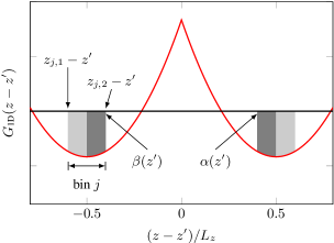
Figure 10: Integration of the spatially averaged kernel for the case where the separation of the charge at $z^{\prime}$ and the bin $j$ covering the interval $[z_{j,1},z_{j,2}]$ is such that periodicity has to be taken into account. $\alpha_{j}(z^{\prime})$ and $\beta_{j}(z^{\prime})$ are the nearest images of the bin boundaries.

Appendix B Validation

In this section, we compare the oxygen-oxygen pair correlation function, $g(r)$, the oxygen-oxygen velocity autocorrelation function, $\text{VACF}(t)$, a cumulative estimate of the dielectric constant, $\epsilon(t)$, and the distance-dependent Kirkwood $g$-factor, $G_{\text{K}}(r)$. We refer to Refs Frenkel and Smit, 2002 and Neumann, 1986b for a detailed discussion and the relevant formulae. All quantities were sampled during 2 ns NVE simulations before imposing the temperature gradients.

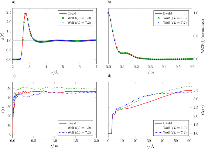
Figure 11: The comparison comprises (a) the oxygen-oxygen pair correlation function, (b) the oxygen-oxygen VACF, (c) a cumulative estimate of the dielectric constant and (d) the distance-dependent Kirkwood $g$-factor.

The results are shown in Figs 11a–d. As we can see, all sets of parameters lead to excellent agreement for $g(r)$ and $\text{VACF}(t)$ (Figs 11a–b). The dielectric constant (Fig. 11c) is well reproduced by the Wolf method with strong damping, whereas weak damping leads to an overestimation. More insight about the structural properties can be gained by looking at $G_{\text{K}}(r)$ in Fig. 11d. For very short distances both sets of parameters for the Wolf method yield a good agreement with Ewald summation. We note that for the weak damping the agreement extends a bit further than for strong damping, which is consistent with our observations for the model system. We also note that the shape of $G_{\text{K}}(r)$ looks different for our elongated box as compared to a cubic box.

References

- Doktycz and Suslick (1990) S. J. Doktycz and K. S. Suslick, Science 247, 1067 (1990).
- Govorov and Richardson (2007) A. O. Govorov and H. H. Richardson, Nano Today 2, 30 (2007).
- Bresme et al. (2008) F. Bresme, A. Lervik, D. Bedeaux, and S. Kjelstrup, Phys. Rev. Lett. 101, 020602 (2008).
- Muscatello et al. (2011) J. Muscatello, F. Römer, J. Sala, and F. Bresme, Phys. Chem. Chem. Phys. 13, 19970 (2011).
- Römer et al. (2012) F. Römer, F. Bresme, J. Muscatello, D. Bedeaux, and J. M. Rubí, Phys. Rev. Lett. 108, 105901 (2012).
- Armstrong and Bresme (2013) J. A. Armstrong and F. Bresme, J. Chem. Phys. 139, 014504 (2013).
- Armstrong, Lervik, and Bresme (2013) J. Armstrong, A. Lervik, and F. Bresme, J. Phys. Chem. B 117, 14817 (2013).
- De Groot and Mazur (1962) S. R. De Groot and P. Mazur, Non-equilibrium thermodynamics, 1st ed. (North-Holland Publishing Company, Amsterdam, 1962).
- Ewald (1921) P. P. Ewald, Ann. Phys. 64, 253 (1921).
- Fennell and Gezelter (2006) C. J. Fennell and J. D. Gezelter, J. Chem. Phys. 124, 234104 (2006).
- Wolf et al. (1999) D. Wolf, P. Keblinski, S. R. Phillpot, and J. Eggebrecht, J. Chem. Phys. 110, 8254 (1999).
- Armstrong, Daub, and Bresme (2015) J. Armstrong, C. D. Daub, and F. Bresme, J. Chem. Phys. 143, 036101 (2015).
- Steinbach and Brooks (1994) P. J. Steinbach and B. R. Brooks, J. Comput. Chem. 15, 667 (1994).
- Zahn, Schilling, and Kast (2002) D. Zahn, B. Schilling, and S. M. Kast, J. Chem. Phys. B 106, 10725 (2002).
- Wu and Brooks (2005) X. Wu and B. R. Brooks, J. Chem. Phys. 122, 44107 (2005).
- Elvira and MacDowell (2014) V. H. Elvira and L. G. MacDowell, J. Chem. Phys. 141, 164108 (2014).
- Fukuda, Yonezawa, and Nakamura (2011) I. Fukuda, Y. Yonezawa, and H. Nakamura, J. Chem. Phys. 134, 164107 (2011).
- Fukuda (2013) I. Fukuda, J. Chem. Phys. 139, 174107 (2013).
- Lamichhane, Gezelter, and Newman (2014) M. Lamichhane, J. D. Gezelter, and K. E. Newman, J. Chem. Phys. 141, 134109 (2014).
- Chen and Weeks (2006) Y.-G. Chen and J. D. Weeks, Proc. Natl. Acad. Sci. 103, 7560 (2006).
- Fanourgakis (2015) G. S. Fanourgakis, J. Phys. Chem. B 119, 1974 (2015).
- Darden, York, and Pedersen (1993) T. Darden, D. York, and L. Pedersen, J. Chem. Phys. 98, 10089 (1993).
- Deserno and Holm (1998) M. Deserno and C. Holm, J. Chem. Phys. 109, 7678 (1998).
- Neumann and Steinhauser (1980) M. Neumann and O. Steinhauser, Mol. Phys. 39, 437 (1980).
- Schreiber and Steinhauser (1992) H. Schreiber and O. Steinhauser, Biochemistry 31, 5856 (1992).
- Feller et al. (1996) S. E. Feller, R. W. Pastor, A. Rojnuckarin, S. Bogusz, and B. R. Brooks, J. Phys. Chem. 100, 17011 (1996).
- Rodgers and Weeks (2008a) J. M. Rodgers and J. D. Weeks, Proc. Natl. Acad. Sci. 105, 19136 (2008a).
- Spohr (1997) E. Spohr, J. Chem. Phys. 107, 6342 (1997).
- Van der Spoel and Van Maaren (2006) D. Van der Spoel and P. J. Van Maaren, J. Chem. Theory Comput. 2, 1 (2006).
- Cisneros et al. (2014) G. A. Cisneros, M. Karttunen, P. Ren, and C. Sagui, Chem. Rev. 114, 779 (2014).
- Muscatello and Bresme (2011) J. Muscatello and F. Bresme, J. Chem. Phys. 135, 234111 (2011).
- Noé Mendoza et al. (2008) F. Noé Mendoza, J. López-Lemus, G. A. Chapela, and J. Alejandre, J. Chem. Phys. 129, 024706 (2008).
- Takahashi, Narumi, and Yasuoka (2011) K. Z. Takahashi, T. Narumi, and K. Yasuoka, J. Chem. Phys. 134, 174112 (2011).
- Rodgers and Weeks (2008b) J. M. Rodgers and J. D. Weeks, J. Phys.: Condens. Matter 20, 494206 (2008b).
- De Leeuw, Perram, and Smith (1980) S. W. De Leeuw, J. W. Perram, and E. R. Smith, Proc. R. Soc. London, Ser. A 373, 27 (1980).
- Neumann, Steinhauser, and Pawley (1984) M. Neumann, O. Steinhauser, and G. S. Pawley, Mol. Phys. 52, 97 (1984).
- Wick, Dang, and Jungwirth (2006) C. D. Wick, L. X. Dang, and P. Jungwirth, J. Chem. Phys. 125, 024706 (2006).
- Wilson, Pohorille, and Pratt (1988) M. A. Wilson, A. Pohorille, and L. R. Pratt, J. Chem. Phys. 88, 3281 (1988).
- Yeh and Berkowitz (1999) I.-C. Yeh and M. L. Berkowitz, J. Chem. Phys. 111, 3155 (1999).
- Glosli and Philpott (1996) J. N. Glosli and M. R. Philpott, Electrochim. Acta 41, 2145 (1996).
- Frenkel and Smit (2002) D. Frenkel and B. Smit, Understanding Molecular Simulation, 2nd ed. (Academic Press, San Diego, 2002).
- Hummer et al. (1999) G. Hummer, L. R. Pratt, A. E. García, and M. Neumann, AIP Conf. Proc. 492, 84 (1999).
- Hummer, Grønbech-Jensen, and Neumann (1998) G. Hummer, N. Grønbech-Jensen, and M. Neumann, J. Chem. Phys. 109, 2791 (1998).
- Berendsen, Grigera, and Straatsma (1987) H. J. C. Berendsen, J. R. Grigera, and T. P. Straatsma, J. Phys. Chem. 91, 6269 (1987).
- Wilson, Pohorille, and Pratt (1989) M. A. Wilson, A. Pohorille, and L. R. Pratt, J. Chem. Phys. 90, 5211 (1989).
- Smith (1998) W. Smith, CCP5 Newsletter 46, 18 (1998).
- Jackson (1998) J. D. Jackson, Classical electrodynamics, 3rd ed. (Wiley, 1998).
- Spaldin (2012) N. A. Spaldin, J. Solid State Chem. 195, 2 (2012).
- Plimpton (1995) S. Plimpton, J. Comput. Phys. 117, 1 (1995).
- Wirnsberger, Frenkel, and Dellago (2015) P. Wirnsberger, D. Frenkel, and C. Dellago, J. Chem. Phys. 143, 124104 (2015).
- Swope et al. (1982) W. C. Swope, H. C. Andersen, P. H. Berens, and K. R. Wilson, J. Chem. Phys. 76, 637 (1982).
- Nosé (1984) S. Nosé, J. Chem. Phys. 81, 511 (1984).
- Hoover (1985) W. G. Hoover, Phys. Rev. A 31, 1695 (1985).
- Yeh and Wallqvist (2011) I.-C. Yeh and A. Wallqvist, J. Chem. Phys. 134, 055109 (2011).
- Neumann (1986a) M. Neumann, Mol. Phys. 57, 97 (1986a).
- Böttcher (1973) C. J. F. Böttcher, Dielectrics in static fields, 2nd ed. (Elsevier Science, 1973) .
- Sokhan and Tildesley (1997) V. P. Sokhan and D. J. Tildesley, Mol. Phys. 92, 625 (1997).
- Stengel, Spaldin, and Vanderbilt (2008) M. Stengel, N. A. Spaldin, and D. Vanderbilt, Nat. Phys. 5, 304 (2009).
- Zhang and Sprik (2016) C. Zhang and M. Sprik, Phys. Rev. B 93, 144201 (2016).
- Neumann (1986b) M. Neumann, J. Chem. Phys. 85, 1567 (1986b).