Extended formalism for simulating compound refractive lens-based x-ray microscopes

Abstract

We present a comprehensive formalism for the simulation and optimisation of CRLs in both condensing and full-field imaging configurations. The approach extends ray transfer matrix analysis to account for x-ray attenuation by the lens material. Closed analytical expressions for critical imaging parameters such as numerical aperture, vignetting, chromatic aberration and focal length are provided for both thin- and thick-lens imaging geometries.

I Introduction

Compound refractive lenses (CRLs) are predominantly used as micro- and nano-focusing lenses in scanning beam microscopy Ice et al. (2011). However, there is a growing use of CRLs as imaging objectives in hard x-ray microscopesSimons et al. (2015). Improving the design of CRLs and their implementation in x-ray microscopes requires a thorough understanding of the optical principles of CRLs as well as convenient and simple analytical expressions for predicting and optimizing imaging performance across a wide variety of optical configurations.

Different approaches have addressed the optical theory of CRLs and CRL-based imaging systems, such as ray-transfer matrices (RTMs) Protopopov and Valiev (1998) (including with Gaussian beams Poulsen and Poulsen (2014)), Monte Carlo ray tracing Sanchez del Rio and Alianelli (2012), wavefront propagation Kohn (2003) and others Lengeler et al. (1999). While each have merits, no single formalism provides the necessary combination of closed analytical expressions, applicability to both condensing and full-field imaging systems, and consideration of the full range of possible geometries (i.e. both the thin and thick-lens imaging conditions).

This work presents a step-by-step derivation of a formalism for CRL-based imaging systems. Intended as a tutorial for beginners in the field, it utilises an RTM approach to model typical x-ray imaging systems in a manner that accounts for both thin-lens and general (i.e. thick-lens) cases. We first introduce the RTM formalism, then derive the the ray path within the CRL. Following this, the CRL formalism is placed in the context of a complete imaging system, and relevant expressions for acceptance functions, resolution and aberration are provided. These expressions are key requirements for efficient parametric optimisation of the CRL and imaging geometry, which could ultimately provide suggestions for future lens development routes.

II The RTM approach

This RTM approach assumes a 1D geometry, valid for axisymmetric and planar CRLs with parabolic curvatures (Fig. 1). The CRL is comprised of $N$ parabolic lenses arranged in a linear array, where each lens has a radius of curvature $R$, aperture $2Y$ and centre-to-centre distance between successive lenslets $T$ so that $Y=\sqrt{RT}$. Lenslets may also have a gap between their apices, given as $T_{\mathrm{web}}$ and a physical lenslet thickness $T_{\mathrm{phys}}<T$. The physical aperture of the lenslet $2Y_{\mathrm{phys}}$ is therefore given by $Y_{\mathrm{phys}}=\sqrt{R(T_{\mathrm{phys}}-T_{\mathrm{web}})}$.

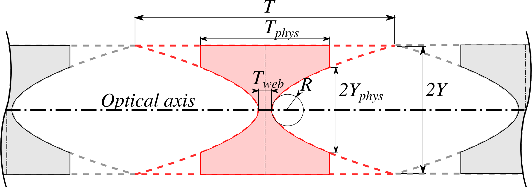
Figure 1: Geometry of the 1D radially symmetric (i.e. axisymmetric) refractive lenslet. A single refracting lenslet element is shown in blue, annotated with symbolic dimensions.

Photons are treated as rays with position $y$ and angle $\alpha$. The RTM then describes an optical system as a matrix $\mathbf{M}$ that transforms an incident ray $(y_{0},\alpha_{0})$ into an exit ray $(y_{1},\alpha_{1})$.

$$\begin{bmatrix}y_{1}\\ \alpha_{1}\end{bmatrix}=\mathbf{M}\begin{bmatrix}y_{0}\\ \alpha_{0}\end{bmatrix}$$ (1)

RTM analysis inherently assumes the following:

1. Paraxial rays, i.e. that the angle between rays and the optical axis is small such that $\sin{(\alpha)}\approx\alpha$ and $\cos{(\alpha)}\approx 1$. This is justified by the weak refractive decrement $\delta$ and consequently small numerical aperture of x-ray CRLs.

2. Thin lenslets, i.e. that the focal length $f$ of each lenslet is much larger than $T$. This is valid for the vast majority of lenslet geometries and the full x-ray energy regime relevant to CRLs (i.e. $E>15$ keV)

3. Reflection and diffraction are negligible. This is well-justified in other approaches e.g. Ref. Schroer et al. (2005)

We first derive the ray transfer matrix of a single, thin lenslet. Its focal length $f$ is given in terms of the lenslet radius $R$ and the refractive decrement $\delta$ as:

$$f=\frac{R}{2\delta}$$ (2)

The corresponding transfer matrix $\mathbf{M}$ can be described as the combination of matrices corresponding to a free space propagation by half the distance between lenslet centres, $T/2$, followed by focusing with focal length $f$ and another free space propagation by $T/2$:

$$\mathbf{M}=\begin{bmatrix}1&T/2\\ 0&1\end{bmatrix}\begin{bmatrix}1&0\\ -1/f&1\end{bmatrix}\begin{bmatrix}1&T/2\\ 0&1\end{bmatrix}=\begin{bmatrix}1-\frac{T}{2f}&f(1-(1-\frac{T}{2f})^{2})\\ \frac{-1}{f}&1-\frac{T}{2f}\end{bmatrix}$$ (3)

The transfer matrix of the CRL, $\mathbf{M}^{N}$ is the combined behaviour of $N$ such lenslets. This can be calculated through the matrix eigendecomposition theorem, where $\mathbf{P}$ is a matrix comprising the eigenvectors of $\mathbf{M}$ and $\mathbf{D}$ is a diagonal matrix comprising the eigenvalues of $\mathbf{M}$.

$$\mathbf{M}^{N}=\mathbf{M}\mathbf{M}...\mathbf{M}=(\mathbf{M})^{N}=\mathbf{P}\mathbf{D}^{N}\mathbf{P^{-1}}$$ (4)

The eigenvalues $E_{\pm}$ - which are a complex conjugate pair if $4f>T$ - may then be expressed as:

$$E_{\pm}=1-\frac{T}{2f}\pm i\sqrt{1-\left(1-\frac{T}{2f}\right)^{2}}=\cos(\varphi)\pm i\sin(\varphi)=\exp{(\pm i\varphi)}$$ (5)

where $\varphi$ is the phase angle of the complex eigenvalues, which may be expressed as:

$$\varphi=\tan^{-1}{\left(\frac{\sqrt{1-\left(1-\frac{T}{2f}\right)^{2}}}{1-\frac{T}{2f}}\right)}\approx\sqrt{\frac{T}{f}}$$ (6)

The corresponding eigenvectors $\mathbf{r}_{\pm}=(y_{\pm},\alpha_{\pm})$ are given by $y_{\pm}=\mp i\alpha_{\pm}f\sin\varphi$. From Eq. 5 the expression for $\mathbf{M}^{N}$ then becomes

$$\begin{split}\mathbf{M^{N}}&=\begin{bmatrix}1&1\\ \frac{1}{if\sin{\varphi}}&\frac{-1}{if\sin{\varphi}}\end{bmatrix}\begin{bmatrix}\exp{(-iN\varphi)}&0\\ 0&\exp{(iN\varphi)}\end{bmatrix}\begin{bmatrix}1&1\\ \frac{1}{if\sin{\varphi}}&\frac{-1}{if\sin{\varphi}}\end{bmatrix}^{-1}\\ &=\begin{bmatrix}\cos{(N\varphi)}&f\sin{\varphi}\sin{(N\varphi)}\\ \frac{-\sin{(N\varphi)}}{f\sin{\varphi}}&\cos{(N\varphi)}\end{bmatrix}\end{split}$$ (7)

Note also that the basic approximation of the RTM approach implies that

$$\begin{split}\sin{\varphi}&=\varphi=\sqrt{\frac{T}{f}}=\frac{1}{\sqrt{2\delta}}\frac{Y}{f}\\ f\sin{\varphi}&=f\varphi=\sqrt{Tf}=\frac{Y}{\sqrt{2\delta}}\end{split}$$ (8)

Here, $\sqrt{2\delta}$ is the critical angle for total external reflection and the numerical aperture for an ideal elliptical lens Als-Nielsen and McMorrow (2010) corresponding to $R=T$ in the parabolic approximation. If there is no space between lenslets, $Y/f$ is half the numerical aperture of one lenslet and $1/(f\varphi)$ is the refractive power of the CRL per unit length Lengeler et al. (1999).

Hence, from Eqs. 7 and 8, $\mathbf{M}^{N}$ can then be expressed as:

$$\mathbf{M}^{N}=\begin{bmatrix}\cos{(N\varphi)}&f\varphi\sin{(N\varphi)}\\ \frac{-\sin{(N\varphi)}}{f\varphi}&\cos{(N\varphi)}\end{bmatrix}$$ (9)

III Derivation of the ray path within CRLs

To calculate the position of a ray at the centre of the $n^{th}$ lenslet, we determine the RTM of the CRL after the lenslet and then back-propagate by half a lenslet distance (i.e. $-T/2$). The ray vector $(y_{n},\alpha_{n})$ as a function of the incident ray $(y_{0},\alpha_{0})$ is then:

$$\begin{bmatrix}y_{n}\\ \alpha_{n}\end{bmatrix}=\begin{bmatrix}1&-T/2\\ 0&1\end{bmatrix}\mathbf{M}^{n}\begin{bmatrix}y_{0}\\ \alpha_{0}\end{bmatrix}=\begin{bmatrix}M_{11}^{n}-\frac{T}{2}M_{21}^{n}&M_{12}^{n}-\frac{T}{2}M_{22}^{n}\\ M_{21}^{n}&M_{22}^{n}\end{bmatrix}\begin{bmatrix}y_{0}\\ \alpha_{0}\end{bmatrix}$$ (10)

Meaning that the lateral position $y_{n}$ is given by:

$$\begin{split}y_{n}&=y_{0}\left(M_{11}^{n}-\frac{T}{2}M_{21}^{n}\right)+\alpha_{0}\left(M_{12}^{n}-\frac{T}{2}M_{22}^{n}\right)\\ &=y_{0}\left(\cos(n\varphi)+\frac{T\sin(n\varphi)}{2f\varphi}\right)+\alpha_{0}\left(f\varphi\sin(n\varphi)-\frac{T}{2}\cos(n\varphi)\right)\\ &=y_{0}\cos{\left(\left(n-\frac{1}{2}\right)\varphi\right)}+\alpha_{0}f\varphi\sin{\left(\left(n-\frac{1}{2}\right)\varphi\right)}\end{split}$$ (11)

Since:

$$\begin{split}\cos(n\varphi)+\frac{T\sin(n\varphi)}{2f\varphi}&=\cos(n\varphi)+\frac{\varphi}{2}\sin(n\varphi)=\cos\left(\left(n-\frac{1}{2}\right)\varphi\right)\\ f\varphi\sin(n\varphi)-\frac{T}{2}\cos(n\varphi)&=f\varphi\left(\sin(n\varphi)-\frac{\varphi}{2}\cos(n\varphi)\right)=f\varphi\sin\left(\left(n-\frac{1}{2}\right)\varphi\right)\end{split}$$ (12)

Trigonometric identities (see Appendix) then give:

$$y_{n}=\sqrt{y_{0}^{2}+\left(\alpha_{0}f\varphi\right)^{2}}\sin\left(\left(n-\frac{1}{2}\right)\varphi+\tan^{-1}\left(\frac{y_{0}}{\alpha_{0}f\varphi}\right)\right)$$ (13)

All rays through the CRL will therefore have a sinusoidal trajectory with a period of $\frac{2\pi Y}{\sqrt{2\delta}}$ that is proportional to the aperture Y. Likewise, for $\alpha_{n}$:

$$\alpha_{n}=\frac{1}{f\varphi}\sqrt{y_{0}^{2}+\left(\alpha_{0}f\varphi\right)^{2}}\sin{\left(n\varphi-\tan^{-1}{\left(\frac{y_{0}}{\alpha_{0}f\varphi}\right)}\right)}\\$$ (14)

If at any point at the trajectory, $\mid y_{n}\mid>Y_{\mathrm{phys}}$, the ray will not be refracted, but either absorbed or contribute to the general background after the lens. From this, the criterion for any ray to participate in the focusing/imaging process becomes:

$$\mid y\mid_{max}\leq Y_{\mathrm{phys}}$$ (15)

As we will show, the imaging condition implies that there at most can be one extremum in practical systems. Hence, the maximum value of $y$, $y_{max}$ is:

$$\mid y\mid_{max}=\max\left(\mid y_{0}\mid,\mid y_{N}\mid,\sqrt{y_{0}^{2}+\left(\alpha_{0}f\varphi\right)^{2}}\right)\\$$ (16)

IV Derivation of focal length

The focal length is the distance from the lens exit $f_{N}$ at which a refracted ray with initial angle $\alpha_{0}=0$ will intersect with the optical axis at $y=0$. This can be conveniently extracted from $\mathbf{M}^{N}$ Gerrard and Burch (2012):

$$f_{N}=-\frac{M^{N}_{11}}{M^{N}_{21}}=f\varphi\cot{(N\varphi)}$$ (17)

Notably, $f_{N}$ is measured from the exit point of the CRL along the optical axis, $NT/2$ from the CRL centre. For small $N\varphi$ the expression above approximates to $f_{N}=\frac{R}{2\delta N}-\frac{NT}{3}$, for which negligible total lens thickness $NT$ reproduces equivalent expressions derived by alternative means, e.g. from Lengeler et al. (1999).

V Derivation of the attenuation profile

For a single lenslet, the attenuation $U$ of a ray passing through a lenslet with linear absorption coefficient $\mu$ and local thickness $t$ at perpendicular distance $y$ from the optical axis can be described by the Beer-Lambert law and a box function $H$, which fully attenuates any ray that exceeds the physical aperture $Y_{\mathrm{phys}}$:

$$U(y)=\exp{[-\mu t(y)]}\times H{\left(\frac{y}{Y_{\mathrm{phys}}}\right)},$$ (18)

where the box function $H$ is:

$$H(x)=\left\{\begin{array}[]{ll}1&\text{for}|x|\leq 1\\ 0&\text{for}|x|>1\end{array}\right.$$ (19)

The paraxial assumption is that the rays propagate each lenslet at a constant distance to the optical axis. The parabolic profile of the lenslets then gives the thickness function $t(y)$:

$$t(y)=T_{\mathrm{web}}+\frac{y^{2}}{R}\hskip 14.22636pt\text{for}\hskip 14.22636pt\mid y\mid<Y_{\mathrm{phys}}$$ (20)

Thus, neglecting the effects of air between lenslets (i.e. assuming high energy x-rays), a single lenslet will attenuate the ray according to:

$$U(y)=\exp{(-\mu T_{\mathrm{web}})}\times\exp{\left(\frac{-\mu y^{2}}{R}\right)}\times H{\left(\frac{y}{Y_{\mathrm{phys}}}\right)}$$ (21)

The cumulative attenuation $U_{N}(y)$ of a ray as it travels through $N$ lenslets is then the product of the individual attenuation contributions from each lenslet:

$$U_{N}=\prod_{n=1}^{N}U(y_{n})=\exp{(-N\mu T_{\mathrm{web}})}\times\exp{\left(\frac{-\mu}{R}\sum_{n=1}^{N}y_{n}^{2}\right)}\times\prod_{n=1}^{N}H{\left(\frac{y_{n}}{Y_{\mathrm{phys}}}\right)},$$ (22)

where $y_{n}$ is the position of the ray at the centre of the $n^{th}$ lenslet. The central expression for $\frac{\mu}{R}\sum_{n=1}^{N}y_{n}^{2}$ is a quadratic term, which can be expressed as:

$$\frac{\mu}{R}\sum_{n=1}^{N}y_{n}^{2}=A_{N}\alpha_{0}^{2}+B_{N}\alpha_{0}y_{0}+C_{N}y_{0}^{2}$$ (23)

The coefficients $A_{N}$, $B_{N}$ and $C_{N}$ are geometric sums which, since $1+\varphi^{2}\approx 1$, have solutions to second order in $\varphi$ (see Appendix for identities):

$$\begin{split}A_{N}&=\frac{\mu}{R}\sum_{n=1}^{N}(M_{12}^{n}-\frac{T}{2}M_{22}^{n})^{2}\\ &=\frac{N\mu(f\varphi)^{2}}{2R}\left(1-\text{sinc}(2N\varphi)\right)\\ &=\frac{N\mu T}{4\delta}\left(1-\text{sinc}(2N\varphi)\right)\end{split}$$ (24)

$$\begin{split}B_{N}&=\frac{\mu}{R}\sum_{n=1}^{N}(M_{11}^{n}-\frac{T}{2}M_{21}^{n})(M_{12}^{n}-\frac{T}{2}M_{22}^{n})\\ &=\frac{\mu}{2\delta}\left(1-\cos(2N\varphi)\right)\end{split}$$ (25)

$$\begin{split}C_{N}&=\frac{\mu}{R}\sum_{n=1}^{N}(M_{11}^{n}-\frac{T}{2}M_{21}^{n})^{2}\\ &=\frac{N\mu}{2R}\left(1+\text{sinc}(2N\varphi)\right)\end{split}$$ (26)

Hence, the attenuation function can be expressed as a 2D tilted Gaussian function with clipped’ boundaries defined by $y_{n}/Y_{\mathrm{phys}}$:

$$U_{N}=\exp{(-N\mu T_{\mathrm{web}})}\times\exp{\left(A_{N}\alpha_{0}^{2}+B_{N}\alpha_{0}y_{0}+C_{N}y_{0}^{2}\right)}\times\prod_{n=1}^{N}H{\left(\frac{y_{n}}{Y_{\mathrm{phys}}}\right)},$$ (27)

VI Derivation of physical and effective apertures

The physical aperture of the CRL corresponds to the spatial acceptance (i.e. in $y$) for a parallel incident beam (i.e. $\alpha_{0}=0$). When $Y_{\mathrm{phys}}$ is sufficiently large, the spatial acceptance has a Gaussian profile in $y$:

$$U_{\mathrm{phys}}=\exp{(-\mu NT)}\exp{\left(\frac{-y_{0}^{2}}{2\sigma_{D}^{2}}\right)}$$ (28)

In such (common) cases, the physical aperture is given by the RMS $\sigma_{D}$:

$$\sigma_{D}=\frac{1}{\sqrt{2C_{N}}}=\sqrt{\frac{R}{\mu N}}\frac{1}{\sqrt{1+\mathrm{sinc}(2N\varphi)}}\\$$ (29)

The effective aperture is the diameter $D_{\mathrm{eff}}$ of a cylindrical pupil function that has the same total transmission as the CRL Lengeler et al. (1999). Its expression is found by solving:

$$\pi\left(\frac{D_{\mathrm{eff}}}{2}\right)^{2}=2\pi\exp{(-\mu NT)}\int_{0}^{Y_{\mathrm{phys}}}{\exp{\left(\frac{-y_{0}^{2}}{2\sigma_{D}^{2}}\right)}y_{0}dy_{0}}$$ (30)

Hence:

$$D_{\mathrm{eff}}=2\sqrt{2}\sigma_{D}\exp{\left(\frac{-\mu NT}{2}\right)}\left[1-\exp{\left(\frac{-Y_{\mathrm{phys}}^{2}}{2\sigma_{D}^{2}}\right)}\right]^{\frac{1}{2}}$$ (31)

VII Derivation of imaging geometries

In an imaging configuration, a ray originating from the sample plane at $(y_{s},\alpha_{s})$ travels through the objective to the detector plane at $(y_{d},\alpha_{d})$. This transformation between the two planes can be expressed as:

$$\begin{bmatrix}y_{d}\\ \alpha_{d}\end{bmatrix}=\begin{bmatrix}1&d_{2}\\ 0&1\end{bmatrix}\mathbf{M^{N}}\begin{bmatrix}1&d_{1}\\ 0&1\end{bmatrix}\begin{bmatrix}y_{s}\\ \alpha_{s}\end{bmatrix}\equiv\mathbf{K}\begin{bmatrix}y_{s}\\ \alpha_{s}\end{bmatrix}$$ (32)

Here, $d_{1}$ is the distance from the sample plane to the entry of the objective, $d_{2}$ is the distance from the exit of the objective to the detector plane and $\mathbf{M^{N}}$ is the RTM for the CRL.

$\mathbf{K}$ is therefore given in terms of $\mathbf{M^{N}}$ as:

$$\mathbf{K}=\begin{bmatrix}M_{11}^{N}+d_{2}M_{21}^{N}&M_{12}^{N}+d_{1}(M_{11}^{N}+d_{2}M_{21}^{N})+d_{2}M_{22}^{N}\\ M_{21}^{N}&d_{1}M_{21}^{N}+M_{22}^{N}\end{bmatrix}$$ (33)

The imaging condition implies that:

$$\begin{bmatrix}0\\ \alpha_{d}\end{bmatrix}=\mathbf{K}\begin{bmatrix}0\\ \alpha_{s}\end{bmatrix}$$ (34)

i.e.:

$$K_{12}=0$$ (35)

Inserting this leads to:

$$f\varphi\sin(N\varphi)+d_{1}\left(\cos(N\varphi)-d_{2}\frac{\sin(N\varphi)}{f\varphi}\right)+d_{2}\cos(N\varphi)=0$$ (36)

This can rewritten as the imaging condition for a thick CRL:

$$\frac{1}{d_{1}}+\frac{1}{d_{2}}-\frac{1}{f_{N}}+\frac{f\varphi\tan(N\varphi)}{d_{1}d_{2}}=0$$ (37)

Next, the magnification of the imaging system $\mathcal{M}$ (a positive number) is defined by:

$$K_{11}=\mathcal{M}=-\frac{y_{d}}{y_{s}}$$ (38)

We therefore have a set of two equations:

$$\begin{split}0&=M_{12}^{N}+d_{1}(M_{11}^{N}+d_{2}M_{21}^{N})+d_{2}M_{22}^{N}\\ -\mathcal{M}&=M_{11}^{N}+d_{2}M_{21}^{N}\end{split}$$ (39)

which can then be solved simultaneously to find expressions for $d_{1}$ and $d_{2}$:

$$d_{1}=-\frac{M_{12}^{N}}{\mathcal{M}}+\frac{M_{11}^{N}M_{22}^{N}}{M_{21}^{N}\mathcal{M}}+\frac{M_{22}^{N}}{M_{21}^{N}}=\frac{f\sin{(\varphi)}}{\sin{(N\varphi)}}\left[\cos{(N\varphi)}+\frac{1}{\mathcal{M}}\right]=f_{N}\left[1+\frac{1}{\mathcal{M}\cos(N\varphi)}\right]$$ (40)

$$d_{2}=-\frac{\mathcal{M}-M_{11}^{N}}{M_{21}^{N}}=\frac{f\sin{(\varphi)}}{\sin{(N\varphi)}}[\cos{(N\varphi)}+\mathcal{M}]=f_{N}\left[1+\frac{\mathcal{M}}{\cos(N\varphi)}\right]$$ (41)

Note that Eqs. 40 and 41 are identical for $\mathcal{M}=1$. Moreover, $d_{1}$ and $d_{2}$ may never be smaller than $f_{N}$. For practical applications, the total sample-to-detector distance: $L=d_{1}+d_{2}+NT$ may be a fixed parameter, implying that we may want to rewrite the imaging condition as an expression in $L$ and $\mathcal{M}$. Addition of these two equations then gives:

$$\frac{L-NT}{f\varphi}\sin(N\varphi)-2\cos(N\varphi)=\mathcal{M}+\frac{1}{\mathcal{M}}$$ (42)

We can rewrite this using trigonometric identities (see Appendix):

$$\sqrt{4+\left(\frac{L-NT}{f\varphi}\right)^{2}}\sin\left(N\varphi-\tan^{-1}(\frac{2f\varphi}{L-NT})\right)=\mathcal{M}+\frac{1}{\mathcal{M}}$$ (43)

Hence, for a given lenslet (i.e. $f$ and $\varphi$), total distance $L$ and magnification $\mathcal{M}$, we can determine the required number of lenses from:

$$N=\frac{1}{\varphi}\left(\sin^{-1}\left(\frac{\mathcal{M}+\frac{1}{\mathcal{M}}}{\sqrt{(\frac{L-NT}{f\varphi})^{2}+4}}\right)+\tan^{-1}\left(\frac{2f\varphi}{L-NT}\right)\right)$$ (44)

Due to the factor of $N$ in the denominator, $N$ should be determined by evaluating the equation twice via, e.g. the fixed-point method.

VIII Derivation of the acceptance functions for imaging systems

The expression for $\mathbf{K}$ (Eq. 33) provides the following expression for $y_{n}$ in terms of the sample plane coordinates $(y_{s},\alpha_{s})$:

$$\begin{split}y_{n}&=\alpha_{s}\left[d_{1}\left(M^{n}_{11}-\frac{T}{2}M^{n}_{21}\right)+M^{n}_{12}-\frac{T}{2}M^{n}_{22}\right]+y_{s}\left(M^{n}_{11}-\frac{T}{2}M^{n}_{21}\right)\\ &=(d_{1}\alpha_{s}+y_{s})\cos{\left[\left(n-\frac{1}{2}\right)\varphi\right]}+f\varphi\alpha_{s}\sin{\left[\left(n-\frac{1}{2}\right)\varphi\right]}\end{split}$$ (45)

The cumulative attenuation for the entire imaging system, $U_{N}$, can be derived in the same manner as for the CRL alone. Temporarily neglecting the physical aperture of the lenslet, this is can be written as:

$$U_{N}(y_{s},\alpha_{s})=\exp{(-N\mu T_{\mathrm{web}})}\times\exp{[-(A_{N}^{*}\alpha_{s}^{2}+B_{N}^{*}y_{s}\alpha_{s}+C_{N}^{*}y_{s}^{2})]}$$ (46)

where the coefficients $A_{N}^{*}$, $B_{N}^{*}$ and $C_{N}^{*}$ are geometrical sums which, using the identities in the Appendix, can be derived as follows:

$$\begin{split}A_{N}^{*}&=\frac{\mu}{R}\sum_{n=1}^{N}\left[d_{1}\left(M^{n}_{11}-\frac{T}{2}M^{n}_{21}\right)+\left(M^{n}_{12}-\frac{T}{2}M^{n}_{22}\right)\right]^{2}\\ &=\frac{\mu}{R}\sum_{n=1}^{N}\left[d_{1}(\cos{(n\varphi)}+\frac{\varphi}{2}\sin{(n\varphi)})+f\varphi\sin{(n\varphi)}-\frac{T}{2}\cos{(n\varphi)}\right]^{2}\\ &=\frac{\mu}{R}\left[d_{1}^{2}+(f\varphi)^{2}\right]\sum_{n=1}^{N}\cos^{2}{\left(\left(n-\frac{1}{2}\right)\varphi-\cot^{-1}{\left(\frac{d_{1}}{f\varphi}\right)}\right)}\\ &=\frac{\mu}{2R}\left[d_{1}^{2}+(f\varphi)^{2}\right]\left[N-1+\frac{1}{\varphi}\sin{\left((N+1)\varphi\right)}\cos{\left((N-1)\varphi-2\cot^{-1}{\left(\frac{d_{1}}{f\varphi}\right)}\right)}\right]\end{split}$$ (47)

$$\begin{split}B_{N}^{*}&=\frac{2\mu}{R}\sum_{n=1}^{N}\left(M^{n}_{11}-\frac{T}{2}M^{n}_{21}\right)\left[d_{1}\left(M^{n}_{11}-\frac{T}{2}M^{n}_{21}\right)+\left(M^{n}_{12}-\frac{T}{2}M^{n}_{22}\right)\right]\\ &=\frac{2\mu}{R}\sum_{n=1}^{N}\left[d_{1}(\cos(n\varphi)+\frac{\varphi}{2}\sin(n\varphi))+f\varphi\sin(n\varphi)-\frac{T}{2}\cos(n\varphi)\right]\left(\cos(n\varphi)+\frac{\varphi}{2}\sin(n\varphi)\right)\\ &=\frac{2\mu}{R}\left[\sum_{n=1}^{N}d_{1}\cos{\left(\left(n-\frac{1}{2}\right)\varphi\right)}+\sum_{n=1}^{N}f\varphi\sin{\left(\left(n-\frac{1}{2}\right)\varphi\right)}\cos{\left(\left(n-\frac{1}{2}\right)\varphi\right)}\right]\\ &=\frac{2\mu}{R}\left[\frac{d_{1}}{2}(N-1)+\sqrt{d_{1}^{2}+(f\varphi)^{2}}\frac{\sin{((N+1)\varphi)}}{2\varphi}\cos{\left((N-1)\varphi-\cot^{-1}{\left(\frac{d_{1}}{f\varphi}\right)}\right)}\right]\end{split}$$ (48)

$$\begin{split}C_{N}^{*}&=\frac{\mu}{R}\sum_{n=1}^{N}\left(M^{n}_{11}-\frac{T}{2}M^{n}_{21}\right)^{2}=C_{N}\\ &=\frac{N\mu}{2R}\left(1+\text{sinc}(2N\varphi)\right)\end{split}$$ (49)

The function $U_{N}(y_{s},\alpha_{s})$ is also a tilted 2D Gaussian. It can be described as the product of a constant term $\exp{(-N\mu T_{\mathrm{web}})}$ and two 1D Gaussian functions:

$$U_{N}(y_{s},\alpha_{s})=\exp{(-N\mu T_{\mathrm{web}})}\times\exp{\left(\frac{-(\alpha_{s}-\gamma y_{s})^{2}}{2\sigma_{a}^{2}}\right)}\times\exp{\left(\frac{-y_{s}^{2}}{2\sigma_{v}^{2}}\right)}$$ (50)

These two functions are the vignetting function, which describes the reduction in brightness from the centre of the optical axis towards its periphery in terms of an RMS $\sigma_{v}$, and the angular acceptance function, which describes the angle over which the lens collects radiation emitted from a point $y_{s}$ on the sample plane. The angular acceptance function has RMS $\sigma_{a}$ and offset $\gamma$. Their individual expressions are derived from the coefficients $A_{N}^{*}$, $B_{N}^{*}$ and $C_{N}^{*}$ in the following subsections.

VIII.1 Angular acceptance

By inspection of Eq. 46, the angular acceptance function is a Gaussian with standard deviation $\sigma_{a}$ given by:

$$\begin{split}\sigma_{a}&=\sqrt{\frac{1}{2A_{N}^{*}}} \\ &=\sqrt{\frac{R}{\mu N[d_{1}^{2}+(f\varphi)^{2}]}}\left[1+\frac{1}{N}-\frac{1}{N\varphi}\sin{((N+1)\varphi)}\cos{\left((N-1)\varphi+2\tan^{-1}{\left(\frac{d_{1}}{f\varphi}\right)}\right)}\right]^{-\frac{1}{2}}\end{split}$$ (51)

The last term is a slowly varying function that asymptotically approaches 1 for $N\varphi\to 0$. The analytical expression for $\gamma$ can similarly be expressed as:

$$\begin{split}\gamma&=\frac{B_{N}^{*}}{2A_{N}^{*}}\\ &=\frac{(f+2d_{1}N)\sqrt{d_{1}^{2}+(f\varphi)^{2}}\cos{\left(2N\varphi+\tan^{-1}{\left(\frac{d_{1}}{f\varphi}\right)}\right)}}{2[d_{1}f+N(d_{1}^{2}+f^{2})]+\frac{1}{\varphi}[d_{1}^{2}+(f\varphi)^{2}]\sin{\left(2N\varphi\right)}}\end{split}$$ (52)

VIII.2 Vignetting

By inspection of Eq. 46, the RMS value $\sigma_{v}$ is given by:

$$\begin{split}\sigma_{v}&=\sqrt{\frac{2A_{N}^{*}}{4A_{N}^{*}C_{N}^{*}-B_{N}^{*2}}}\\ &=\frac{\delta}{\mu\sigma_{a}}\left[(N\varphi)^{2}-\sin^{2}{(N\varphi)}\right]^{-\frac{1}{2}}\end{split}$$ (53)

IX Derivation of spatial resolution

The spatial resolution, $\Delta y_{d}$, is the minimum distance two objects can be separated while still being ‘distinguishable’ by the imaging system. While the Rayleigh criterion Born and Wolf (1999) provides a simple and effective approximation for this, it is not applicable to systems with Gaussian pupil (i.e. attenuation) functions. Instead, we must first derive the point-spread function (PSF) of the system, then determine the minimum resolvable distance between two such PSFs.

In an ideal imaging configuration, the PSF is simply the Fourier transform of the pupil function, $P(y_{0})$ Born and Wolf (1999):

$$PSF(y_{s})=\mathcal{F}(P(y_{0}))$$ (54)

where the pupil function is the acceptance of a ray emanating from the centre of the field-of-view, derived from Eq. 50:

$$P(y_{0})=\exp{\left(\frac{-y_{0}^{2}}{2\sigma_{a}^{2}d_{1}^{2}}\right)}\times H\left(\frac{y_{0}}{Y_{\mathrm{pup}}}\right)$$ (55)

Here, $Y_{\mathrm{pup}}\equiv Y_{\mathrm{phys}}/\sqrt{1+\left(f\varphi/d_{1}\right)^{2}}$. For a wavenumber $k=2\pi/\lambda$ at x-ray wavelength $\lambda$, and ignoring constant prefactors, the point-spread intensity function at the source plane, $PSF(y_{s})$, is then given by:

$$\begin{split}PSF(y_{s})&=\left\lvert\int_{-\infty}^{\infty}{P(y_{0})\exp{\left[-i\frac{k}{d_{1}}y_{0}y_{s}\right]}}\mathrm{d}y_{0}\right\rvert^{2}\\ &=\exp{\left(-k^{2}\sigma_{a}^{2}y_{s}^{2}\right)}\times\left[\operatorname{erf}{\left(\frac{Y_{\mathrm{pup}}+ik\sigma_{a}^{2}y_{s}}{\sqrt{2}\sigma_{a}}\right)}+\operatorname{erf}{\left(\frac{Y_{\mathrm{pup}}-ik\sigma_{a}^{2}y_{s}}{\sqrt{2}\sigma_{a}}\right)}\right]^{2}\end{split}$$ (56)

The resolution can then be defined by the the separation distance between two PSFs corresponding to a contrast ratio of $C$ (where $C$ is small when the contrast is poor). Using Eq. 56, this can be determined by numerically solving:

$$\frac{PSF(0)+PSF(\Delta y_{s})}{PSF(\frac{\Delta y_{s}}{2})+PSF(-\frac{\Delta y_{s}}{2})}=1-C$$ (57)

In the case of absorption-limited (i.e. Gaussian) CRLs, this gives a function in terms of $\lambda$, $\sigma_{a}$ and $C$:

$$\Delta y_{d}=\sqrt{0.06905-0.1019\log{(1-C)}}\frac{\lambda}{\sigma_{a}}$$ (58)

X Derivation of chromatic aberration

The refractive decrement $\delta$ is approximately inversely proportional to the square of the of the x-ray energy. Hence, compared to $\delta_{0}$ at a nominal energy $E_{0}$, the actual $\delta$ at energy $E$ will be:

$$\delta\approx\delta_{0}\frac{E_{0}^{2}}{E^{2}}=\frac{\delta_{0}}{(1+\epsilon)^{2}}$$ (59)

Where $\epsilon$ is a (small) normalised energy perturbation such that $E/E_{0}=1+\epsilon$. This energy dependence of $\delta$ means that the values for $f$ and $\varphi$ in the formalism are similarly chromatic. Their new values values are:

$$\varphi=\frac{\varphi_{0}}{1+\epsilon}\approx\varphi_{0}(1-\epsilon),\qquad f=f_{0}(1+\epsilon)^{2}\approx f_{0}(1+2\epsilon)$$ (60)

A ray originating from the sample at $y_{s}=0$ will strike the detector at $y_{d}$ according to:

$$y_{d}=\alpha_{s}\left[(d_{1}+d_{2})\cos{(N\varphi)}+\left(f\varphi-\frac{d_{1}d_{2}}{f\varphi}\right)\sin{(N\varphi)}\right]$$ (61)

If we are in an ideal imaging condition at $E=E_{0}$, then $y_{d,0}=y_{s}=0$. However, if $E\neq E_{0}$ then the ray will strike the detector at $y_{d}\neq y_{s}=0$. The dependence of $y_{d}$ on $\epsilon$ is found by substituting the chromatic expressions for $\phi$ and $f$ and Taylor expanding to first order in $\epsilon$:

$$y_{d}=y_{d,0}+d_{\mathrm{ch}}\epsilon\alpha_{s}=d_{\mathrm{ch}}\epsilon\alpha_{s}$$ (62)

where:

$$d_{\mathrm{ch}}=\frac{N\varphi_{0}[d_{1}d_{2}-(f_{0}\varphi_{0})^{2}]\cos{(N\varphi_{0})}+[d_{1}d_{2}+(f_{0}\varphi_{0})^{2}+f_{0}N\varphi_{0}^{2}(d_{1}+d_{2})]\sin{(N\varphi_{0})}}{f_{0}\varphi_{0}}$$ (63)

To calculate the intensity of a chromatic ray, we first consider that the incident ray will have an intensity at the sample $I_{\epsilon}$ defined by the chromatic distribution of the source. In many cases this is Gaussian with an RMS bandwidth $\sigma_{e}$:

$$I_{\epsilon}=I_{0}\frac{1}{\sqrt{2\pi}\sigma_{e}}\exp{\left(\frac{-\epsilon^{2}}{2\sigma_{e}^{2}}\right)}$$ (64)

The ray will then be attenuated by the material in the lens as a function of its incident angle $\alpha_{s}$. From the formalism we know that this is a Gaussian attenuation function with RMS width $\sigma_{a}$ given by:

$$U(\alpha_{s})=\exp{\left(\frac{-\alpha_{s}^{2}}{2\sigma_{a}^{2}}\right)}$$ (65)

Thus, the intensity of the ray at the detector position, $I_{d}$, will be:

$$I_{d}(\epsilon,\alpha_{s})=I_{\epsilon}\times U(\alpha_{s})=I_{0}\frac{1}{\sqrt{2\pi}\sigma_{e}}\exp{\left(\frac{-\epsilon^{2}}{2\sigma_{e}^{2}}\right)}\times\exp{\left(\frac{-\alpha_{s}^{2}}{2\sigma_{a}^{2}}\right)}$$ (66)

From Eq. 61, we can calculate the initial angle of a ray given its $\epsilon$ and $y_{d}$ as $\alpha_{s}=y_{d}/(d_{\mathrm{ch}}\epsilon)$. Substituting this into Eq. 66 then gives the spatio-chromatic intensity distribution at the detector:

$$I_{d}(\epsilon,y_{d})=I_{0}\frac{1}{\sqrt{2\pi}\sigma_{e}}\exp{\left(\frac{-\epsilon^{2}}{2\sigma_{e}^{2}}\right)}\times\exp{\left[\frac{-y_{d}^{2}}{2(\sigma_{a}d_{ch}\epsilon)^{2}}\right]}$$ (67)

Normalising $y_{d}$ by the system magnification $\mathcal{M}$ then gives the perceived chromatic point-spread in the sample coordinates, $y_{s}$:

$$I_{s}(\epsilon,y_{d})=I_{0}\frac{1}{\sqrt{2\pi}\sigma_{e}}\exp{\left(\frac{-\epsilon^{2}}{2\sigma_{e}^{2}}\right)}\times\exp{\left[\frac{-y_{s}^{2}}{2(\sigma_{a}d_{ch}\epsilon\mathcal{M})^{2}}\right]}$$ (68)

So the chromatic point-spread function ($PSF_{\mathrm{chr}}$) is then obtained by integrating $I_{d}$ across $\epsilon$:

$$\begin{split}PSF_{\mathrm{ch}}&=I_{0}\frac{1}{\sqrt{2\pi}\sigma_{e}}\int_{-\infty}^{\infty}{\exp{\left(\frac{-\epsilon^{2}}{2\sigma_{e}^{2}}\right)}\times\exp{\left(\frac{-y_{s}^{2}}{2(\sigma_{a}d_{\mathrm{ch}}\mathcal{M}\epsilon)^{2}}\right)}\mathrm{d}\epsilon}\\ &=I_{0}\exp{\left(\frac{-\lvert y_{s}\rvert}{\sigma_{e}\sigma_{a}\mathcal{M}d_{\mathrm{ch}}}\right)}\end{split}$$ (69)

Which is a Laplacian distribution with characteristic width:

$$\sigma_{\mathrm{ch}}=\sigma_{a}\sigma_{e}\mathcal{M}d_{\mathrm{ch}}$$ (70)

XI Conclusions

In conclusion, this formalism describes the focusing and attenuation properties of CRLs and CRL-based imaging systems. Specifically, it provides closed analytical expressions for crucial optical parameters including vignetting, angular acceptance and both chromatic and diffraction-limited spatial resolution.

The expressions provided are general and may be used on the vast majority of imaging configurations, including at the ‘thick-lens limit’, where working distances are very small compared to the length of the CRL.

Moreover, these expressions are highly suited for fast computation as well as algebraic manipulation, and may therefore be used for analytical and parametric optimisation.

*

Appendix A Trigonometric Identities

Throughout this work, we will make use of the following identities:

$$a\cos(\theta)+b\sin(\theta)=\sqrt{a^{2}+b^{2}}\cos\left(\theta-\cot^{-1}\left(\frac{a}{b}\right)\right)=\sqrt{a^{2}+b^{2}}\sin\left(\theta+\tan^{-1}\left(\frac{a}{b}\right)\right)$$ (71)

And:

$$\sum_{n=1}^{N}\sin^{2}(n\theta+d)=\frac{1}{2}\left(N+1-\frac{\sin((N+1)\theta)}{\sin\theta}\cos(N\theta+2d)\right)$$ (72)

$$\sum_{n=1}^{N}\cos^{2}(n\theta+d)=\frac{1}{2}\left(N-1+\frac{\sin((N+1)\theta)}{\sin\theta}\cos(N\theta+2d)\right)$$ (73)

$$\sum_{n=1}^{N}\cos(n\theta+d)\sin(n\theta+d)=\frac{1}{2}\left(\frac{\sin((N+1)\theta)}{\sin\theta}\sin(N\theta+2d)\right)$$ (74)

Furthermore, we utilize that $\tan^{-1}(x)=\cot^{-1}\left(\frac{1}{x}\right)\approx x$ for $x\ll 1$

Finally we mention the following two identities

$$\sin(\cot^{-1}(x))=\frac{1}{\sqrt{1+x^{2}}}$$ (75)

$$\cos(\cot^{-1}(x))=\frac{x}{\sqrt{1+x^{2}}}$$ (76)

References

Ice et al. (2011)
G. E. Ice,
J. D. Budai, and
J. W. L. Pang,
Science 334,
1234 (2011).
Simons et al. (2015)
H. Simons,
A. King,
W. Ludwig,
C. Detlefs,
W. Pantleon,
S. Schmidt,
I. Snigireva,
A. Snigirev, and
H. F. Poulsen,
Nat. Commun. 6,
6098 (2015).
Protopopov and Valiev (1998)
V. V. Protopopov
and K. A.
Valiev, Opt. Commun.
151, 297 (1998).
Poulsen and Poulsen (2014)
S. O. Poulsen and
H. F. Poulsen,
Metall. Mater. Trans. A 45A,
4772 (2014).
Kohn (2003)
V. G. Kohn, J.
Exp. Theor. Phys. 97, 204
(2003).
Lengeler et al. (1999)
B. Lengeler,
C. Schroer,
J. Tümmler,
B. Benner,
M. Richwin,
A. Snigirev,
I. Snigireva,
and
M. Drakopoulos,
J. of Synchrotron Radiat. 6,
1153 (1999),
URL http://dx.doi.org/10.1107/S0909049599009747.
Schroer et al. (2005)
C. G. Schroer,
O. Kurapova,
J. Patommel,
P. Boye,
J. Feldkamp,
B. Lengeler,
M. Burghammer,
C. Riekel,
L. Vince,
A. van der Hart,
et al., Appl. Phys. Lett.
87, 124103
(2005).
Als-Nielsen and McMorrow (2010)
J. Als-Nielsen and
D. McMorrow,
Elements of modern X-ray physics
(Wiley, 2010).
Gerrard and Burch (2012)
A. Gerrard and
J. M. Burch,
Introduction to matrix methods in optics
(Courier Corporation, 2012).
Born and Wolf (1999)
M. Born and
E. Wolf,
Principles of Optics (Cambridge
University Press, 1999), 7th ed.