licensedusgovmixed \isbn978-1-4503-4944-4/17/04\acmPrice$15.00 http://dx.doi.org/10.1145/3052973.3053009
Practical Black-Box Attacks against Machine Learning
Abstract
Machine learning (ML) models, e.g., deep neural networks (DNNs), are vulnerable to adversarial examples: malicious inputs modified to yield erroneous model outputs, while appearing unmodified to human observers. Potential attacks include having malicious content like malware identified as legitimate or controlling vehicle behavior. Yet, all existing adversarial example attacks require knowledge of either the model internals or its training data. We introduce the first practical demonstration of an attacker controlling a remotely hosted DNN with no such knowledge. Indeed, the only capability of our black-box adversary is to observe labels given by the DNN to chosen inputs. Our attack strategy consists in training a local model to substitute for the target DNN, using inputs synthetically generated by an adversary and labeled by the target DNN. We use the local substitute to craft adversarial examples, and find that they are misclassified by the targeted DNN. To perform a real-world and properly-blinded evaluation, we attack a DNN hosted by MetaMind, an online deep learning API. We find that their DNN misclassifies 84.24% of the adversarial examples crafted with our substitute. We demonstrate the general applicability of our strategy to many ML techniques by conducting the same attack against models hosted by Amazon and Google, using logistic regression substitutes. They yield adversarial examples misclassified by Amazon and Google at rates of 96.19% and 88.94%. We also find that this black-box attack strategy is capable of evading defense strategies previously found to make adversarial example crafting harder.
1 Introduction
A classifier is a ML model that learns a mapping between inputs and a set of classes. For instance, a malware detector is a classifier taking executables as inputs and assigning them to the benign or malware class. Efforts in the security [5, 2, 9, 18] and machine learning [14, 4] communities exposed the vulnerability of classifiers to integrity attacks. Such attacks are often instantiated by adversarial examples: legitimate inputs altered by adding small, often imperceptible, perturbations to force a learned classifier to misclassify the resulting adversarial inputs, while remaining correctly classified by a human observer. To illustrate, consider the following images, potentially consumed by an autonomous vehicle [13]:
![[Uncaptioned image]](/html/1602.02697/assets/fig/stop-sign.png)
![[Uncaptioned image]](/html/1602.02697/assets/fig/yield-sign.png)
To humans, these images appear to be the same: our biological classifiers (vision) identify each image as a stop sign. The image on the left [13] is indeed an ordinary image of a stop sign. We produced the image on the right by adding a precise perturbation that forces a particular DNN to classify it as a yield sign, as described in Section 5.2. Here, an adversary could potentially use the altered image to cause a car without failsafes to behave dangerously. This attack would require modifying the image used internally by the car through transformations of the physical traffic sign. Related works showed the feasibility of such physical transformations for a state-of-the-art vision classifier [6] and face recognition model [11]. It is thus conceivable that physical adversarial traffic signs could be generated by maliciously modifying the sign itself, e.g., with stickers or paint.
In this paper, we introduce the first demonstration that black-box attacks against DNN classifiers are practical for real-world adversaries with no knowledge about the model. We assume the adversary (a) has no information about the structure or parameters of the DNN, and (b) does not have access to any large training dataset. The adversary’s only capability is to observe labels assigned by the DNN for chosen inputs, in a manner analog to a cryptographic oracle.
Our novel attack strategy is to train a local substitute DNN with a synthetic dataset: the inputs are synthetic and generated by the adversary, while the outputs are labels assigned by the target DNN and observed by the adversary. Adversarial examples are crafted using the substitute parameters, which are known to us. They are not only misclassified by the substitute but also by the target DNN, because both models have similar decision boundaries.
This is a considerable departure from previous work, which evaluated perturbations required to craft adversarial examples using either: (a) detailed knowledge of the DNN architecture and parameters [2, 4, 9, 14], or (b) an independently collected training set to fit an auxiliary model [2, 4, 14]. This limited their applicability to strong adversaries capable of gaining insider knowledge of the targeted ML model, or collecting large labeled training sets. We release assumption (a) by learning a substitute: it gives us the benefit of having full access to the model and apply previous adversarial example crafting methods. We release assumption (b) by replacing the independently collected training set with a synthetic dataset constructed by the adversary with synthetic inputs and labeled by observing the target DNN’s output.
Our threat model thus corresponds to the real-world scenario of users interacting with classifiers hosted remotely by a third-party keeping the model internals secret. In fact, we instantiate our attack against classifiers automatically trained by MetaMind, Amazon, and Google. We are able to access them only after training is completed. Thus, we provide the first correctly blinded experiments concerning adversarial examples as a security risk.
We show that our black-box attack is applicable to many remote systems taking decisions based on ML, because it combines three key properties: (a) the capabilities required are limited to observing output class labels, (b) the number of labels queried is limited, and (c) the approach applies and scales to different ML classifier types (see Section 7), in addition to state-of-the-art DNNs. In contrast, previous work failed to simultaneously provide all of these three key properties [4, 14, 12, 15, 18]. Our contributions are:
-
•
We introduce in Section 4 an attack against black-box DNN classifiers. It crafts adversarial examples without knowledge of the classifier training data or model. To do so, a synthetic dataset is constructed by the adversary to train a substitute for the targeted DNN classifier.
-
•
In Section 5, we instantiate the attack against a remote DNN classifier hosted by MetaMind. The DNN misclassifies of the adversarial inputs crafted.
-
•
The attack is calibrated in Section 6 to (a) reduce the number of queries made to the target model and (b) maximize misclassification of adversarial examples.
-
•
We generalize the attack to other ML classifiers like logistic regression. In Section 7, we target models hosted by Amazon and Google. They misclassify adversarial examples at rates of and .
-
•
Section 8 shows that our attack evades defenses proposed in the literature because the substitute trained by the adversary is unaffected by defenses deployed on the targeted oracle model to reduce its vulnerability.
-
•
In Appendix B, we provide an intuition of why adversarial examples crafted with the substitute also mislead target models by empirically observing that substitutes have gradients correlated to the target’s.
Disclosure: We disclosed our attacks to MetaMind, Amazon, and Google. Note that no damage was caused as we demonstrated control of models created for our own account.
2 About Deep Neural Networks
We provide preliminaries of deep learning to enable understanding of our threat model and attack. We refer readers interested to the more detailed presentation in [3].
A deep neural network (DNN), as illustrated in Figure 1, is a ML technique that uses a hierarchical composition of parametric functions to model an input . Each function for is modeled using a layer of neurons, which are elementary computing units applying an activation function to the previous layer’s weighted representation of the input to generate a new representation. Each layer is parameterized by a weight vector (we omit the vector notation) impacting each neuron’s activation. Such weights hold the knowledge of a DNN model and are evaluated during its training phase, as detailed below. Thus, a DNN defines and computes:
| (1) |
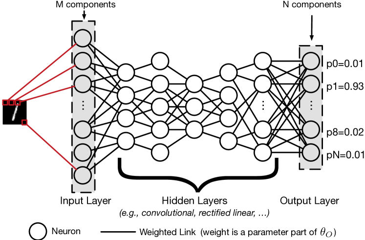
The training phase of a DNN learns values for its parameters . We focus on classification tasks, where the goal is to assign inputs a label among a predefined set of labels. The DNN is given a large set of known input-output pairs and it adjusts weight parameters to reduce a cost quantifying the prediction error between the prediction and the correct output . The adjustment is typically performed using techniques derived from the backpropagation algorithm. Briefly, such techniques successively propagate error gradients with respect to network parameters from the network’s output layer to its input layer.
During the test phase, the DNN is deployed with a fixed set of parameters to make predictions on inputs unseen during training. We consider classifiers: the DNN produces a probability vector encoding its belief of input being in each of the classes (cf. Figure 1). The weight parameters hold the model knowledge acquired by training. Ideally, the model should generalize and make accurate predictions for inputs outside of the domain explored during training. However, attacks manipulating DNN inputs with adversarial examples showed this is not the case in practice [4, 9, 14].
3 Threat Model
A taxonomy of adversaries against DNN classifiers is found in [9]. In our work, the adversary seeks to force a classifier to misclassify inputs in any class different from their correct class. To achieve this, we consider a weak adversary with access to the DNN output only. The adversary has no knowledge of the architectural choices made to design the DNN, which include the number, type, and size of layers, nor of the training data used to learn the DNN’s parameters. Such attacks are referred to as black box, where adversaries need not know internal details of a system to compromise it.
Targeted Model: We consider attackers targeting a multi-class DNN classifier. It outputs probability vectors, where each vector component encodes the DNN’s belief of the input being part of one of the predefined classes. We consider the ongoing example of a DNN classifying images, as shown in Figure 1. Such DNNs can be used to classify handwritten digits into classes associated with digits from 0 to 9, images of objects in a fixed number of categories, or images of traffic signs into classes identifying its type (STOP, yield, …).
Adversarial Capabilities: The oracle is the targeted DNN. Its name refers to the only capability of the adversary: accessing the label for any input by querying oracle . The output label is the index of the class assigned the largest probability by the DNN:
| (2) |
where is the -th component of the probability vector output by DNN . Distinguishing between labels and probabilities makes adversaries realistic (they more often have access to labels than probabilities) but weaker: labels encode less information about the model’s learned behavior. Accessing labels produced by the DNN is the only capability assumed in our threat model. We do not have access to the oracle internals or training data.
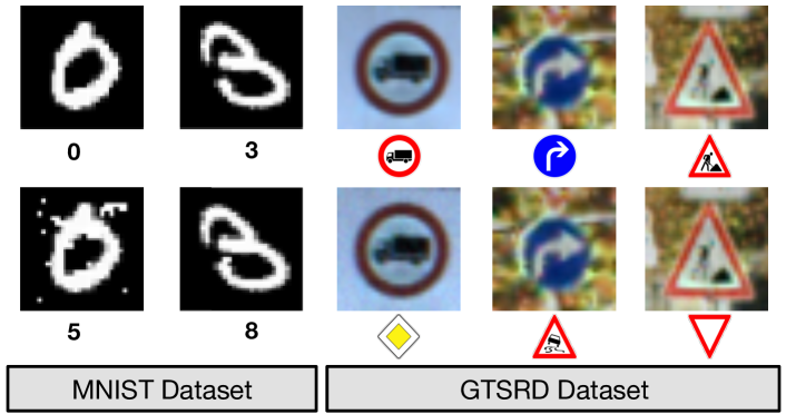
Adversarial Goal: We want to produce a minimally altered version of any input , named adversarial sample, and denoted , misclassified by oracle : . This corresponds to an attack on the oracle’s output integrity. Adversarial samples solve the following optimization problem:
| (3) |
Examples of adversarial samples can be found in Figure 2. The first row contains legitimate samples and the second corresponding adversarial samples that are misclassified. This misclassification must be achieved by adding a minimal perturbation so as to evade human detection. Even with total knowledge of the architecture used to train model and its parameters resulting from training, finding such a minimal perturbation is not trivial, as properties of DNNs preclude the optimization problem from being linear or convex. This is exacerbated by our threat model: removing knowledge of model ’s architecture and training data makes it harder to find a perturbation such that holds.
In Appendix C, we give a presentation of attacks conducted in related threat models—with stronger assumptions.
4 Black-Box Attack Strategy
We introduce our black-box attack. As stated in Section 3, the adversary wants to craft inputs misclassified by the ML model using the sole capability of accessing the label assigned by classifier for any chosen input . The strategy is to learn a substitute for the target model using a synthetic dataset generated by the adversary and labeled by observing the oracle output. Then, adversarial examples are crafted using this substitute. We expect the target DNN to misclassify them due to transferability between architectures [14, 4]
To understand the difficulty of conducting the attack under this threat model, recall Equation 3 formalizing the adversarial goal of finding a minimal perturbation that forces the targeted oracle to misclassify. A closed form solution cannot be found when the target is a non-convex ML model: e.g., a DNN. The basis for most adversarial attacks [4, 9, 14] is to approximate its solution using gradient-based optimization on functions defined by a DNN. Because evaluating these functions and their gradients requires knowledge of the DNN architecture and parameters, such an attack is not possible under our black-box scenario. It was shown that adversaries with access to an independently collected labeled training set from the same population distribution than the oracle could train a model with a different architecture and use it as a substitute [14]: adversarial examples designed to manipulate the substitute are often misclassified by the targeted model. However, many modern machine learning systems require large and expensive training sets for training. For instance, we consider models trained with several tens of thousands of labeled examples. This makes attacks based on this paradigm unfeasible for adversaries without large labeled datasets.
In this paper, we show black-box attacks can be accomplished at a much lower cost, without labeling an independent training set. In our approach, to enable the adversary to train a substitute model without a real labeled dataset, we use the target DNN as an oracle to construct a synthetic dataset. The inputs are synthetically generated and the outputs are labels observed from the oracle. Using this synthetic dataset, the attacker builds an approximation of the model learned by the oracle. This substitute network is then used to craft adversarial samples misclassified by Indeed, with its full knowledge of the substitute DNN parameters, the adversary can use one of the previously described attacks [4, 9] to craft adversarial samples misclassified by . As long as the transferability property holds between and , adversarial samples crafted for will also be misclassified by . This leads us to propose the following strategy:
-
1.
Substitute Model Training: the attacker queries the oracle with synthetic inputs selected by a Jacobian-based heuristic to build a model approximating the oracle model ’s decision boundaries.
-
2.
Adversarial Sample Crafting: the attacker uses substitute network to craft adversarial samples, which are then misclassified by oracle due to the transferability of adversarial samples.
4.1 Substitute Model Training
Training a substitute model approximating oracle is challenging because we must: (1) select an architecture for our substitute without knowledge of the targeted oracle’s architecture, and (2) limit the number of queries made to the oracle in order to ensure that the approach is tractable. Our approach, illustrated in Figure 3, overcomes these challenges mainly by introducing a synthetic data generation technique, the Jacobian-based Dataset Augmentation. We emphasize that this technique is not designed to maximize the substitute DNN’s accuracy but rather ensure that it approximates the oracle’s decision boundaries with few label queries.

Substitute Architecture: This factor is not the most limiting as the adversary must at least have some partial knowledge of the oracle input (e.g., images, text) and expected output (e.g., classification). The adversary can thus use an architecture adapted to the input-output relation. For instance, a convolutional neural network is suitable for image classification. Furthermore, we show in Section 6 that the type, number, and size of layers used in the substitute DNN have relatively little impact on the success of the attack. Adversaries can also consider performing an architecture exploration and train several substitute models before selecting the one yielding the highest attack success.
Generating a Synthetic Dataset: To better understand the need for synthetic data, note that we could potentially make an infinite number of queries to obtain the oracle’s output for any input belonging to the input domain. This would provide us with a copy of the oracle. However, this is simply not tractable: consider a DNN with input components, each taking discrete values among a set of possible values, the number of possible inputs to be queried is . The intractability is even more apparent for inputs in the continuous domain. Furthermore, making a large number of queries renders the adversarial behavior easy to detect.
A natural alternative is to resort to randomly selecting additional points to be queried. For instance, we tried using Gaussian noise to select points on which to train substitutes. However, the resulting models were not able to learn by querying the oracle. This is likely due to noise not being representative of the input distribution. To address this issue, we thus introduce a heuristic efficiently exploring the input domain and, as shown in Sections 5 and 6, drastically limits the number of oracle queries. Furthermore, our technique also ensures that the substitute DNN is an approximation of the targeted DNN i.e. it learns similar decision boundaries.
The heuristic used to generate synthetic training inputs is based on identifying directions in which the model’s output is varying, around an initial set of training points. Such directions intuitively require more input-output pairs to capture the output variations of the target DNN . Therefore, to get a substitute DNN accurately approximating the oracle’s decision boundaries, the heuristic prioritizes these samples when querying the oracle for labels. These directions are identified with the substitute DNN’s Jacobian matrix , which is evaluated at several input points (how these points are chosen is described below). Precisely, the adversary evaluates the sign of the Jacobian matrix dimension corresponding to the label assigned to input by the oracle: . To obtain a new synthetic training point, a term is added to the original point . We name this technique Jacobian-based Dataset Augmentation. We base our substitute training algorithm on the idea of iteratively refining the model in directions identified using the Jacobian.
Substitute DNN Training Algorithm: We now describe the five-step training procedure outlined in Algorithm 1:
-
•
Initial Collection (1): The adversary collects a very small set of inputs representative of the input domain. For instance, if the targeted oracle classifies handwritten digits, the adversary collects 10 images of each digit 0 through 9. We show in Section 5 that this set does not necessarily have to come from the distribution from which the targeted oracle was trained.
-
•
Architecture Selection (2): The adversary selects an architecture to be trained as the substitute . Again, this can be done using high-level knowledge of the classification task performed by the oracle (e.g., convolutional networks are appropriate for vision)
-
•
Substitute Training: The adversary iteratively trains more accurate substitute DNNs by repeating the following for :
-
–
Labeling (3): By querying for the labels output by oracle , the adversary labels each sample in its initial substitute training set .
-
–
Training (4): The adversary trains the architecture chosen at step (2) using substitute training set in conjunction with classical training techniques.
-
–
Augmentation (5): The adversary applies our augmentation technique on the initial substitute training set to produce a larger substitute training set with more synthetic training points. This new training set better represents the model’s decision boundaries. The adversary repeats steps (3) and (4) with the augmented set .
-
–
Step (3) is repeated several times to increase the substitute DNN’s accuracy and the similarity of its decision boundaries with the oracle. We introduce the term substitute training epoch, indexed with , to refer to each iteration performed. This leads to this formalization of the Jacobian-based Dataset Augmentation performed at step (5) of our substitute training algorithm to find more synthetic training points:
| (4) |
where is a parameter of the augmentation: it defines the size of the step taken in the sensitive direction identified by the Jacobian matrix to augment the set into .
4.2 Adversarial Sample Crafting
Once the adversary trained a substitute DNN, it uses it to craft adversarial samples. This is performed by implementing two previously introduced approaches described in [4, 9]. We provide an overview of the two approaches, namely the Goodfellow et al. algorithm and the Papernot et al. algorithm. Both techniques share a similar intuition of evaluating the model’s sensitivity to input modifications in order to select a small perturbation achieving the misclassification goal111Our attack can be implemented with other adversarial example algorithms. We focus on these two in our evaluation..
Goodfellow et al. algorithm: This algorithm is also known as the fast gradient sign method [4]. Given a model with an associated cost function , the adversary crafts an adversarial sample for a given legitimate sample by computing the following perturbation:
| (5) |
where perturbation is the sign of the model’s cost function 222As described here, the method causes simple misclassification. It has been extended to achieve chosen target classes. gradient. The cost gradient is computed with respect to using sample and label as inputs. The value of the input variation parameter factoring the sign matrix controls the perturbation’s amplitude. Increasing its value increases the likelihood of being misclassified by model but on the contrary makes adversarial samples easier to detect by humans. In Section 6, we evaluate the impact of parameter on the successfulness of our attack.
Papernot et al. algorithm: This algorithm is suitable for source-target misclassification attacks where adversaries seek to take samples from any legitimate source class to any chosen target class [9]. Misclassification attacks are a special case of source-target misclassifications, where the target class can be any class different from the legitimate source class. Given model , the adversary crafts an adversarial sample for a given legitimate sample by adding a perturbation to a subset of the input components .
To choose input components forming perturbation , components are sorted by decreasing adversarial saliency value. The adversarial saliency value of component for an adversarial target class is defined as:
| (6) |
where matrix is the model’s Jacobian matrix. Input components are added to perturbation in order of decreasing adversarial saliency value until the resulting adversarial sample is misclassified by . The perturbation introduced for each selected input component can vary: greater perturbation reduce the number of components perturbed to achieve misclassification.
Each algorithm has its benefits and drawbacks. The Goodfellow algorithm is well suited for fast crafting of many adversarial samples with relatively large perturbations thus potentially easier to detect. The Papernot algorithm reduces perturbations at the expense of a greater computing cost.
5 Validation of the Attack
We validate our attack against remote and local classifiers. We first apply it to target a DNN remotely provided by MetaMind, through their API333The API can be accessed online at www.metamind.io that allows a user to train classifiers using deep learning. The API returns labels produced by the DNN for any given input but does not provide access to the DNN. This corresponds to the oracle described in our threat model. We show that:
-
•
An adversary using our attack can reliably force the DNN trained using MetaMind on MNIST [7] to misclassify of adversarial examples crafted with a perturbation not affecting human recognition.
-
•
A second oracle trained locally with the German Traffic Signs Recognition Benchmark (GTSRB) [13], can be forced to misclassify more than of altered inputs without affecting human recognition.
5.1 Attack against the MetaMind Oracle
Description of the Oracle: We used the MNIST handwritten digit dataset to train the DNN [7]. It comprises training and test images of handwritten digits. The task associated with the dataset is to identify the digit corresponding to each image. Each x grayscale sample is encoded as a vector of pixel intensities in the interval and obtained by reading the image pixel matrix row-wise.
We registered for an API key on MetaMind’s website, which gave us access to three functionalities: dataset upload, automated model training, and model prediction querying. We uploaded the samples included in the MNIST training set to MetaMind and then used the API to train a classifier on the dataset. We emphasize that training is automated: we have no access to the training algorithm, model architecture, or model parameters. All we are given is the accuracy of the resulting model, computed by MetaMind using a validation set created by isolating of the training samples. Details can be found on MetaMind’s website.
Training took 36 hours to return a classifier with a accuracy. This performance cannot be improved as we cannot access or modify the model’s specifications and training algorithm. Once training is completed, we could access the model predictions, for any input of our choice, through the API. Predictions take the form of a class label. This corresponds to the threat model described in Section 3.
Initial Substitute Training Sets: First, the adversary collects an initial substitute training set. We describe two such sets used to attack the MetaMind oracle:
-
•
MNIST subset: This initial substitute training set is made of samples from the MNIST test set. They differ from those used by the oracle for training as test and training sets are distinct. We assume adversaries can collect such a limited sample set under the threat model described in Section 3 with minimal knowledge of the oracle task: here, handwritten digit classification.
-
•
Handcrafted set: To ensure our results do not stem from similarities between the MNIST test and training sets, we also consider a handcrafted initial substitute training set. We handcrafted samples by handwriting digits for each class between and with a laptop trackpad. We then adapted them to the MNIST format of x grayscale pixels. Some are shown below.
Substitute DNN Training: The adversary uses the initial substitute training sets and the oracle to train subsitute DNNs. Our substitute architecture A, a standard for image classification, is described in Table 13 (cf. appendix). The substitute DNN is trained on our machine for substitute epochs. During each of these epochs, the model is trained for epochs from scratch with a learning rate of and momentum of . Between substitute epochs, we perform a Jacobian-based dataset augmentation with a step size of to generate additional synthetic training data, which we label using the MetaMind oracle.
The accuracy of the two substitute DNNs is reported in Figure 4. It is computed with the MNIST test set (minus the samples used in the first initial substitute training set). The adversary does not have access to this full test set: we solely use it to analyze our results. The two substitute DNNs respectively achieve a and accuracy on the MNIST test set after substitute training epochs. These accuracies fall short of current state-of-the-art accuracies on this task. However, the adversary has access to a limited number of samples (in this case instead of for state-of-the-art models). Furthermore, the adversarial goal is to craft adversarial samples misclassified by the oracle. Instead of learning a substitute DNN with optimal accuracy, the adversary is interested in learning a substitute capable of mimicking the oracle decision boundaries.
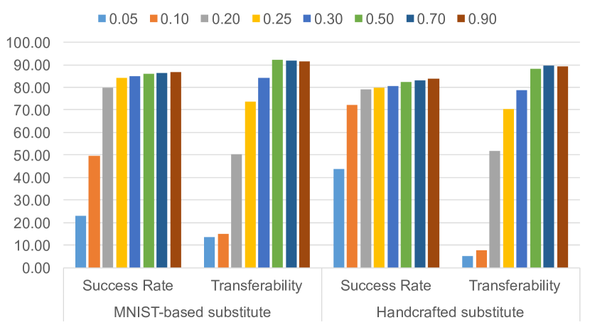
Adversarial Sample Crafting: Using the substitute DNNs, we then craft adversarial samples using Goodfellow’s algorithm. We decided to use the samples from the MNIST test set as our legitimate samples.444Again, adversaries do not need access to the dataset and can use any legitimate sample of their choice to craft adversarial samples. We use it in order to show that expected inputs can be misclassified on a large scale. We evaluate sample crafting using two metrics: success rate and transferability. The success rate is the proportion of adversarial samples misclassified by the substitute DNN. Our goal is to verify whether these samples are also misclassified by the oracle or not. Therefore, the transferability of adversarial samples refers to the oracle misclassification rate of adversarial samples crafted using the substitute DNN.
Figure 5 details both metrics for each substitute DNN and for several values of the input variation (cf. Equation 5). Transferability reaches for the first substitute DNN and for the second, with input variations of . Our attack strategy is thus effectively able to severely damage the output integrity of the MetaMind oracle. Using the substitute training set handcrafted by the adversary limits the transferability of adversarial samples when compared to the substitute set extracted from MNIST data, for all input variations except . Yet, the transferability of both substitutes is similar, corroborating that our attack can be executed without access to any of the oracle’s training data.
| Substitute | Initial Substitute Training Set from | |
| Epoch | MNIST test set | Handcrafted digits |
| 0 | ||
| 1 | ||
| 2 | ||
| 3 | ||
| 4 | ||
| 5 | ||
| 6 | ||
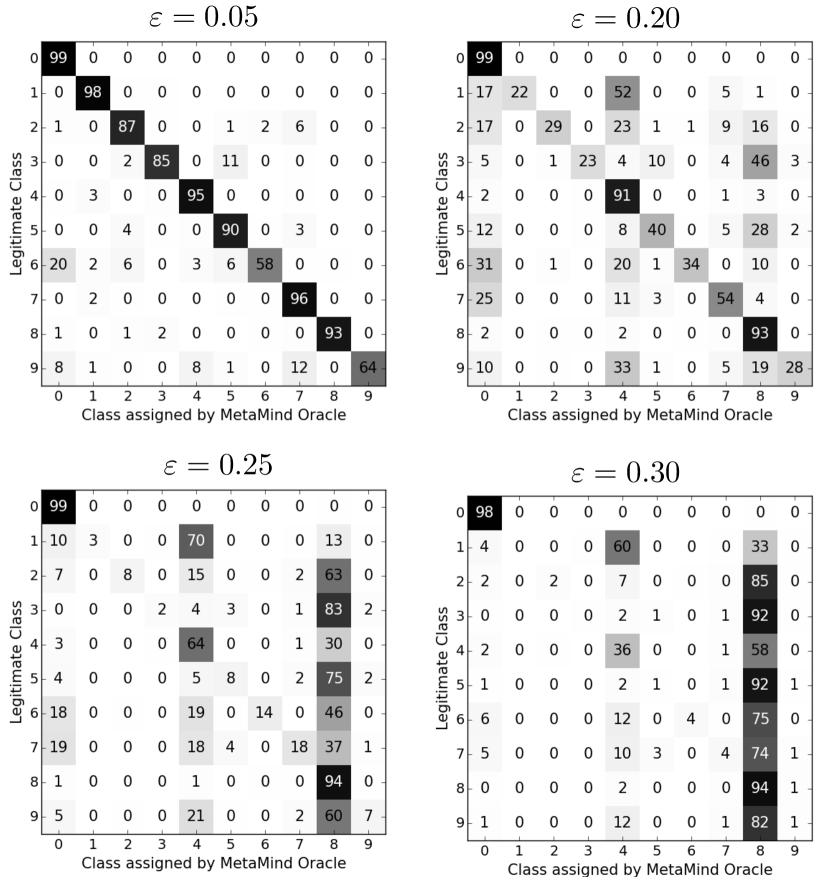
To analyze the labels assigned by the MetaMind oracle, we plot confusion matrices for adversarial samples crafted using the first substitute DNN with values of . In Figure 6, rates on the diagonal indicate the proportion of samples correctly classified by the oracle for each of the classes. Off-diagonal values are the proportion of samples misclassified in a wrong class. For instance, cell in the third matrix indicates that instances of a are classified as a by the oracle when perturbed with an input variation of . Confusion matrices converge to most samples being classified as s and s as increases. This could be due to DNNs more easily classifying inputs in these classes [9].
5.2 Attacking an oracle for the GTSRB
We now validate our attack on a different dataset, using an oracle trained locally to recognize traffic signs on the GTSRB dataset. The attack achieves higher transferability rates at lower distortions compared to the MNIST oracle.
Oracle Description: The GTSRB dataset is an image collection consisting of 43 traffic signs [13]. Images vary in size and are RGB-encoded. To simplify, we resize images to x pixels, recenter them by subtracting the mean component, and rescale them by factoring their standard deviations out. We keep images for our training set and for our validation set (out of the available), and for our test set (out of ). We train the oracle on our machine, using the DNN B from Table 13 (cf. appendix), for epochs with a learning rate of and a momentum of (both decayed by every epochs).
Substitute DNN Training: The adversary uses two initial substitute training sets extracted from the GTSRB test set. The first includes the first samples and the second the first . The number of initial samples is higher than for MNIST substitutes as inputs have a higher dimensionality. We train three substitute architectures C, D, and E (cf. Table 13) using the oracle for substitute training epochs with a Jacobian-based dataset augmentation parameter of . Substitute C and E where trained with the sample initial substitute training set and achieve a accuracy. Substitute D was trained with the initial set of samples. Its accuracy of is lower than C and E.
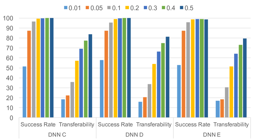
Adversarial Crafting: We use Goodfellow’s algorithm with between and to craft adversarial samples from the test set. Results are shown in Figure 7. Adversarial samples crafted with variations are more transferable than those crafted with the same for MNIST models. This is likely due to the higher input dimensionality— components instead of —which means almost times more perturbation is applied with the same . Nevertheless, with success rates higher than and transferability rates ranging from to for , which is hard to distinguish for humans, the attack is successful. The transferability of adversarial samples crafted using substitute DNN D is comparable or higher than corresponding samples for DNNs C and E, despite being less accurate (trained with less samples). This emphasizes that there is no strong correlation between substitute accuracy and transferability.
6 Attack Algorithm Calibration
Having shown in Section 5 that an adversary can force an MNIST oracle from MetaMind, and a GTSRB oracle trained locally, to misclassify inputs, we now perform a parameter space exploration of both attack steps–the substitute DNN training and the adversarial sample crafting. We explore the following questions: “(1) How can substitute training be fine-tuned to improve adversarial sample transferability?” and (2) “For each adversarial sample crafting strategies, which parameters optimize transferability?”. We found that:
-
•
In Section 6.1, we show that the choice of substitute DNN architecture (number of layers, size, activation function, type) has a limited impact on adversarial sample transferability. Increasing the number of epochs, after the substitute DNN has reached an asymptotic accuracy, does not improve adversarial sample transferability.
-
•
At comparable input perturbation magnitude, the Goodfellow and Papernot algorithms have similar transferability rates (see Section 6.2).
In this section, we use an oracle trained locally to limit querying of the MetaMind API. We train architecture A (cf. Table 13) for epochs with a learning parameter and a momentum (both decayed by every epochs).
6.1 Calibrating Substitute DNN Training
We first seek to quantify the impact of substitute training algorithm parameters on adversarial sample transferability and introduce a refinement to reduce oracle querying.
Choosing an Architecture: We train substitute DNNs A and F to M (cf. Table 13) using samples from the MNIST test set as the substitute training set. During each of the substitute training epochs, the DNN is trained for epochs from scratch. Between epochs, synthetic data is added to the training set using Jacobian-based dataset augmentations with step . The substitute architectures differ from the oracle’s by the type, number, and size of layers. In Table 1, we report the accuracy of each architecture after and substitute training epochs, as well as the adversarial sample transferability after 6 epochs. Adversarial samples are crafted using the Goodfellow algorithm with an input variation of (which we justify later). The last column of Table 1 shows that the choice of architecture has a limited impact on adversarial sample transferability, and therefore on the attack success. The most important transferability drop follows from removing all convolutional layers. Changing the hidden layer activation function from rectified linear to a sigmoid does not impact transferability significantly.
Choosing the number of substitute epochs: Another tunable parameter is the number of epochs for which substitute DNNs are trained. Intuitively, one would hypothesize that the longer we train the substitute, the more samples labeled using the oracle are included in the substitute training set, thus the higher the transferability of adversarial samples will be. This intuition is confirmed only partially by our experiments on substitute DNN A. We find that for for input variations , the transferability is slightly improved by a rate between to , but for variations , the transferability is slightly degraded by less than .
| DNN | Accuracy | Accuracy | Transferability |
| ID | () | () | () |
| A | |||
| F | |||
| G | |||
| H | |||
| I | |||
| J | |||
| K | |||
| L | |||
| M | 76.04 |
Setting the step size: We trained substitute A using different Jacobian-based dataset augmentation step sizes . Increasing or decreasing the step size (from used in the rest of this paper) does not modify the substitute accuracy by more than . Larger step sizes decrease convergence stability while smaller values yield slower convergence. However, increasing step size negatively impacts adversarial sample transferability : for instance with a step size of compared to , the transferability rate for is instead of and for , instead of .
However, having the step size periodically alternating between positive and negative values improves the quality of the oracle approximation made by the substitute. This could be explained by the fact that after a few substitute epochs, synthetic inputs are outside of the input domain and are thus clipped to produce an acceptable input. We introduce an iteration period after which the step size is multiplied by . Thus, the step size is now replaced by:
| (7) |
where is set to be the number of epochs after which the Jacobian-based dataset augmentation does not lead any substantial improvement in the substitute. A grid search can also be performed to find an optimal value for the period . We also experimented with a decreasing grid step amplitude , but did not find that it yielded substantial improvements.
Reducing Oracle Querying: We apply reservoir sampling [16] to reduce the number of queries made to the oracle. This is useful when learning substitutes in realistic environments, or when interacting with paid APIs, where the number of label queries an adversary can make without exceeding a quota or being detected by a defender is limited. Reservoir sampling is a technique that randomly select samples from a list of samples. The total number of samples in the list can be both very large and unknown. We use it to select new inputs before a Jacobian-based dataset augmentation. This prevents the exponential growth of queries made to the oracle at each augmentation. At iterations (the first iterations are performed normally), when considering the previous set of substitute training inputs, we select inputs from to be augmented in . Using reservoir sampling ensures that each input in has an equal probability to be augmented in . The number of queries made to the oracle is reduced from for the vanilla Jacobian-based augmentation to with reservoir sampling. In Section 7, we show that using reservoir sampling to reduce the number of synthetic training inputs does not significantly degrade the substitute accuracy.
6.2 Adversarial Sample Crafting
We compare the transferability of adversarial samples produced by each algorithm introduced previously [4, 9], to elect the strongest technique under our threat model.
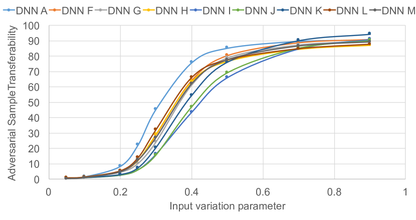
Goodfellow’s algorithm: Recall from Equation 5 the perturbation computed in the Goodfellow attack. Its only parameter is the variation added in the direction of the gradient sign. We use the same architecture set as before to quantify the impact of on adversarial sample transferability. In Figure 8, architecture A outperforms all others: it is a copy of the oracle’s and acts as a baseline. Other architectures have asymptotic transferability rates ranging between and , confirming that the substitute architecture choice has a limited impact on transferability. Increasing the value of above yields little improvement in transferability and should be avoided to guarantee indistinguishability of adversarial samples to humans.
Papernot’s algorithm: This algorithm is fine-tuned by two parameters: the maximum distortion and the input variation . The maximum distortion555In [9], the algorithm stopped perturbing when the input reached the target class. Here, we force the algorithm to continue perturbing until it changed input components. defines the number of input components that are altered in perturbation . The input variation, similarly to the Goodfellow algorithm, controls the amount of change induced to altered input components.
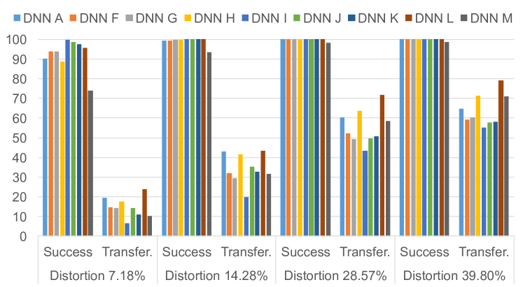
We first evaluate the impact of the maximum distortion on adversarial sample transferability. For now, components selected to be perturbed are increased by . Intuitively, increasing the maximum distortion makes adversarial samples more transferable. Higher distortions increase the misclassification confidence of the substitute DNN, and also increases the likelihood of the oracle misclassifying the same sample. These results are reported in Figure 9. Increasing distortion from to improves transferability: at a distortion, the average transferability across all architectures is whereas at a distortion, the average transferability is at .
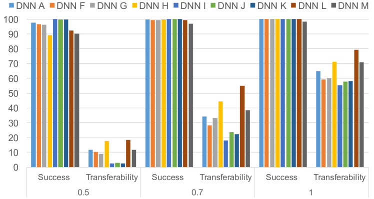
We now quantify the impact of the variation introduced to each input component selected in . We find that reducing the input variation from to significantly degrades adversarial sample transferability, approximatively by a factor of 2 (cf. Figure 10). This is explained by the fixed distortion parameter , which prevents the crafting algorithm from increasing the number of components altered to compensate for the reduced effectiveness yielded by the smaller .
Comparing Crafting Algorithms: To compare the two crafting strategies and their differing perturbation styles fairly, we compare their success rate given a fixed L1 norm of the introduced perturbation , which can be defined as:
| (8) |
where is the number of input components selected in the perturbation , and the input variation introduced to each component perturbed. For the Goodfellow algorithm, we always have , whereas for the Papernot algorithm, values vary for both and . For instance, corresponds to a Goodfellow algorithm with and a Papernot algorithm with and . Corresponding transferability rates can be found in Table 1 and Figure 9 for our running set of architectures. Performances are comparable with some DNNs performing better with one algorithm and others with the other. Thus, the choice of algorithm depends on acceptable perturbations: e.g., all features perturbed a little vs. few features perturbed a lot. Indeed, the Goodfellow algorithm gives more control on while the Papernot algorithm gives more control on .
7 Generalization of the Attack
So far, all substitutes and oracles considered were learned with DNNs. However, no part of the attack limits its applicability to other ML techniques. For instance, we show that the attack generalizes to non-differentiable target oracles like decision trees. As pointed out by Equation 4, the only limitation is placed on the substitute: it must model a differentiable function—to allow for synthetic data to be generated with its Jacobian matrix. We show below that:
-
•
Substitutes can also be learned with logistic regression.
-
•
The attack generalizes to additional ML models by: (1) learning substitutes of 4 classifier types (logistic regression, SVM, decision tree, nearest neighbors) in addition to DNNs, and (2) targeting remote models hosted by Amazon Web Services and Google Cloud Prediction with success rates of and after queries to train the substitute.
7.1 Generalizing Substitute Learning
We here show that our approach generalizes to ML models that are not DNNs. Indeed, we learn substitutes for 4 representative types of ML classifiers in addition to DNNs: logistic regression (LR), support vector machines (SVM), decision trees (DT), and nearest neighbor (kNN). All of these classifiers are trained on MNIST, with no feature engineering (i.e. directly on raw pixel values) as done in Section 5.
Whereas we previously trained all of our substitutes using DNNs only, we now use both DNNs and LR as substitute models. The Jacobian-based dataset augmentation described in the context of DNNs is easily adapted to logistic regression: the later is analog to the softmax layer frequently used by the former when outputting probability vectors. We use samples from the MNIST test set as the initial substitute training set and use the two refinements introduced in Section 6: a periodic step size and reservoir sampling.
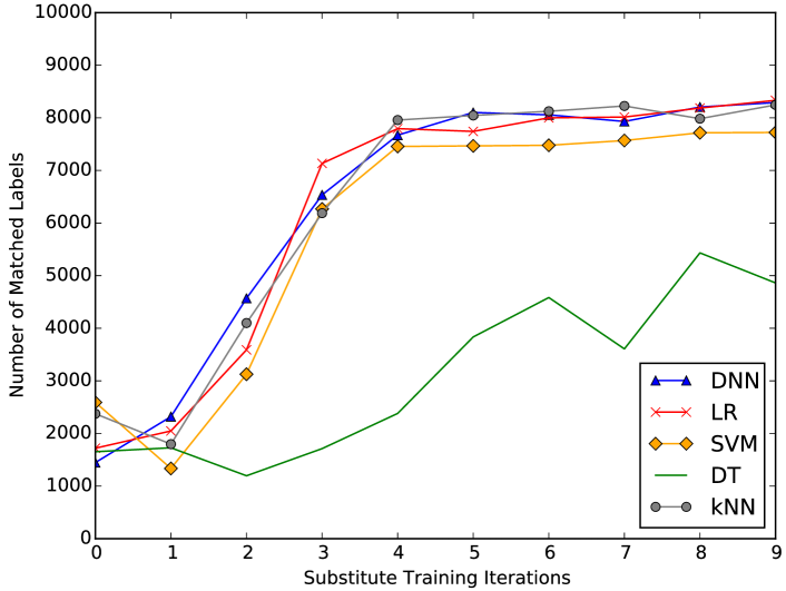
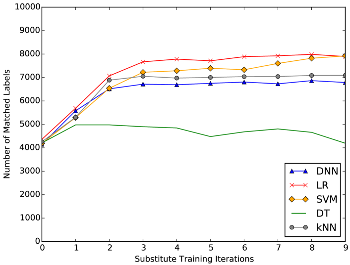
Figure 11(a) and 11(b) plot for each iteration the share of samples on which the substitute DNNs and LRs agree with predictions made by the oracle they are approximating. This proportion is estimated by comparing labels assigned to the test set by the substitutes and oracles before each iteration of the Jacobian-based dataset augmentation. All substitutes are able to approximate the corresponding oracle at rates higher between and after iterations (to the exception of the decision tree oracle, which could be due to its non-continuity). LR substitute accuracies are generally lower than those of DNN substitutes, except when targeting the LR and SVM oracles where LR substitutes outperform DNN ones. However, LR substitutes are computationally more efficient and reach their asymptotic match rate faster, after iterations, corresponding to oracle queries.
Table 2 quantifies the impact of refinements introduced in Section 6 on results reported in Figure 11(a) and 11(b). The periodic step size (PSS) increases the oracle approximation accuracy of substitutes. After epochs, a substitute DNN trained with PSS matches of the DNN oracle labels, whereas the vanilla substitute DNN matches only . Similarly, the LR substitute with PSS matches of the LR oracle labels while the vanilla substitute matched . Using reservoir sampling (RS) reduces oracle querying. For instance, iterations with RS ( and ) make queries to the oracle instead of without RS. This decreases the substitute accuracy, but when combined with PSS it remains superior to the vanilla substitutes. For instance, the vanilla substitute matched of the DNN oracle labels, the PSS one , and the PSS with RS one . Simarly, the vanilla LR substitute matched of the SVM oracle labels, the PSS one , and the PSS with RS .
| Substitute | DNN | LR | SVM | DT | kNN |
|---|---|---|---|---|---|
| DNN | 78.01 | 82.17 | 79.68 | 62.75 | 81.83 |
| DNN+PSS | 89.28 | 89.16 | 83.79 | 61.10 | 85.67 |
| DNN+PSS+RS | 82.90 | 83.33 | 77.22 | 48.62 | 82.46 |
| LR | 64.93 | 72.00 | 71.56 | 38.44 | 70.74 |
| LR+PSS | 69.20 | 84.01 | 82.19 | 34.14 | 71.02 |
| LR+PSS+RS | 67.85 | 78.94 | 79.20 | 41.93 | 70.92 |
| Amazon | |||||
|---|---|---|---|---|---|
| Epochs | Queries | DNN | LR | DNN | LR |
| 800 | 87.44 | 96.19 | 84.50 | 88.94 | |
| 6,400 | 96.78 | 96.43 | 97.17 | 92.05 | |
| 2,000 | 95.68 | 95.83 | 91.57 | 97.72 | |
.
7.2 Attacks against Amazon & Google oracles
Amazon oracle: To train a classifier on Amazon Machine Learning,666https://aws.amazon.com/machine-learning, we uploaded a CSV version of the MNIST dataset to a S3 bucket. We then loaded the data, selected the multi-class model type, and keept default configuration settings. The process took a few minutes and produced a classifier achieving a test set accuracy. We cannot improve the accuracy due to the automated nature of training. We then activate real-time predictions to query the model for labels from our machine with the provided API. Although probabilities are returned, we discard them and retain only the most likely label—as stated in our threat model (Section 3).
Google oracle: The procedure to train a classifier on Google’s Cloud Prediction API777https://cloud.google.com/prediction/ is similar to Amazon’s. We upload the CSV file with the MNIST training data to Google Cloud Storage. We then train a model using the Prediction API. The only property we can specify is the expected multi-class nature of our model. We then evaluate the resulting model on the MNIST test set. The API reports an accuracy of on this test set for the model trained.
Substitute Training: By augmenting an initial training set of test set samples, we train a DNN and LR substitute for each of the two oracles. We measure success as the rate of adversarial samples misclassified by the corresponding oracle, among the produced from the test set using the fast gradient sign method with parameter . These rates, computed after dataset augmentation iterations, are reported in Table 3. Results reported in the last row use both a periodic step size and reservoir sampling (hence the reduced number of queries made to train the substitute).
Experimental Results: With a misclassification rate for a perturbation crafted using a LR substitute trained with oracle queries, the model hosted by Amazon is easily misled. The model trained by Google is somewhat more robust to adversarial samples, but is still vulnerable to a large proportion of samples: of adversarial samples produced in the same conditions are misclassified. A careful read of the documentation indicated that the model trained by Amazon is a multinomial logistic regression.888docs.aws.amazon.com/machine-learning As pointed out in [4], shallow models like logistic regression are unable to cope with adversarial samples and learn robust classifiers. This explains why the attack is very successful and the LR substitute performs better than the DNN substitute. We were however not able to find the ML technique Google uses.
The last row of Table 3 shows how combining periodic step sizes with reservoir sampling allow us to reduce querying of both oracles during substitute training, while crafting adversarial samples with higher transferability to the target classifier. Indeed, querying is reduced by a factor larger than from to queries, while misclassification decreases only from to for the Amazon DNN substitute. It is still larger than the rate of achieved after queries by the substitute learned without the refinements. Similarly, the misclassification rate of the Google LR substitute is —compared to with the original method after epochs, confirming the result.
8 Defense Strategies
The two types of defense strategies are: (1) reactive where one seeks to detect adversarial examples, and (2) proactive where one makes the model itself more robust. Our attack is not more easily detectable than a classic adversarial example attack. Indeed, oracle queries may be distributed among a set of colluding users, and as such remain hard to detect. The defender may increase the attacker’s cost by training models with higher input dimensionality or modeling complexity, as our experimental results indicate that these two factors increase the number of queries required to train substitutes. In the following, we thus only analyze our attack in the face of defenses that seek to make the (oracle) model robust.
Many potential defense mechanisms fall into a category we call gradient masking. These techniques construct a model that does not have useful gradients, e.g., by using a nearest neighbor classifier instead of a DNN. Such methods make it difficult to construct an adversarial example directly, due to the absence of a gradient, but are often still vulnerable to the adversarial examples that affect a smooth version of the same model. Previously, it has been shown that nearest neighbor was vulnerable to attacks based on transferring adversarial examples from smoothed nearest neighbors[4].
We show a more general flaw in the category of gradient masking. Even if the defender attempts to prevent attacks by not publishing the directions in which the model is sensitive, these directions can be discovered by other means, in which case the same attack can still succeed. We show that the black-box attack based on transfer from a substitute model overcomes gradient masking defenses. No fully effective defense mechanism is known, but we study the two with the greatest empirical success so far: adversarial training [4, 14], and defensive distillation for DNNs [10].
| Training | Attack | OO | S S | S O |
|---|---|---|---|---|
.
Adversarial training: It was shown that injecting adversarial examples throughout training increases the robustness of significantly descriptive models, such as DNNs [4, 14, 17]. We implemented an approximation of this defense using the Google Prediction API. Since the API does not support the generation of adversarial examples at every step of training, as a correct implementation of adversarial training would do, we instead inject a large amount of adversarial examples infrequently. After training in this way, the model has a misclassification rate of on the unperturbed test set, but the adversarial misclassification rate rises to when . To evaluate this defense strategy using a correct implementation, we resort to training the oracle locally, using our own codebase that includes support for generating adversarial examples at each step. After each training batch, we compute and train on adversarial examples generated with the fast gradient sign method before starting training on the next batch of the original training data. Results are given in Table 4. We observe that for , the defense can be evaded using the black-box attack with adversarial examples crafted on the substitute and misclassified by the oracle at rates up to . However, for , the black-box attack is not effective anymore. Therefore, making a machine learning model robust to small and infinitesimal perturbations of its inputs is an example of gradient masking and can be evaded using our substitute-based black-box approach. However, making the model robust to larger and finite perturbations prevents the black-box attack. To confirm this hypothesis, we now show that defensive distillation, which makes the model robust to infinitesimal perturbations, can be evaded by the black-box approach.

Defensive distillation: Due to space constraints, we refer readers to [10] for a detailed presentation of defensive distillation, which is an alternative defense. Because the remotely hosted APIs we study here do not implement defensive distillation or provide primitives that could be used to implement it, we are forced to evaluate this defense on a locally trained oracle. Therefore, we train a distilled model as described in [10] to act as our MNIST oracle.
We train several variants of the DNN architecture A at different distillation temperatures . For each of them, we measure the success of the fast gradient sign attack (i.e., the Goodfellow et al. algorithm) directly performed on the distilled oracle—as a baseline corresponding to a white-box attack—and using a substitute DNN trained with synthetic data as described throughout the present paper. The results are reported in Figure 12 for different values of the input variation parameter on the horizontal axis. We find that defensive distillation defends against the fast gradient sign method when the attack is performed directly on the distilled model, i.e. in white-box settings. However, in black-box settings using the attack introduced in the present paper, the fast gradient sign method is found to be successful regardless of the distillation temperature used by the oracle. We hypothesize that this is due to the way distillation defends against the attack: it reduces the gradients in local neighborhoods of training points. However, our substitute model is not distilled, and as such possesses the gradients required for the fast gradient sign method to be successful when computing adversarial examples.
Defenses which make models robust in a small neighborhood of the training manifold perform gradient masking: they smooth the decision surface and reduce gradients used by adversarial crafting in small neighborhoods. However, using a substitute and our black-box approach evades these defenses, as the substitute model is not trained to be robust to the said small perturbations. We conclude that defending against finite perturbations is a more promising avenue for future work than defending against infinitesimal perturbations.
9 Conclusions
We introduced an attack, based on a novel substitute training algorithm using synthetic data generation, to craft adversarial examples misclassified by black-box DNNs. Our work is a significant step towards relaxing strong assumptions about adversarial capabilities made by previous attacks. We assumed only that the adversary is capable of observing labels assigned by the model to inputs of its choice. We validated our attack design by targeting a remote DNN served by MetaMind, forcing it to misclassify of our adversarial samples. We also conducted an extensive calibration of our algorithm and generalized it to other ML models by instantiating it against classifiers hosted by Amazon and Google, with success rates of and . Our attack evades a category of defenses, which we call gradient masking, previously proposed to increase resilience to adversarial examples. Finally, we provided an intuition for adversarial sample transferability across DNNs in Appendix B.
References
- [1] Marco Barreno, et al. Can machine learning be secure? In Proceedings of the 2006 ACM Symposium on Information, Computer and Communications Security.
- [2] Battista Biggio, et al. Evasion attacks against machine learning at test time. In Machine Learning and Knowledge Discovery in Databases, pages 387–402. Springer, 2013.
- [3] Ian Goodfellow, et al. Deep learning. Book in preparation for MIT Press (www.deeplearningbook.org), 2016.
- [4] Ian J Goodfellow, et al. Explaining and harnessing adversarial examples. In Proceedings of the International Conference on Learning Representations, 2015.
- [5] Ling Huang, et al. Adversarial machine learning. In Proceedings of the 4th ACM workshop on Security and artificial intelligence, pages 43–58, 2011.
- [6] Alexey Kurakin, et al. Adversarial examples in the physical world. arXiv preprint arXiv:1607.02533, 2016.
- [7] Yann LeCun et al. The mnist database of handwritten digits, 1998.
- [8] Erich L. Lehmann, et al. Testing Statistical Hypotheses. Springer Texts in Statistics, August 2008.
- [9] Nicolas Papernot, et al. The limitations of deep learning in adversarial settings. In Proceedings of the 1st IEEE European Symposium on Security and Privacy, 2016.
- [10] Nicolas Papernot, et al. Distillation as a defense to adversarial perturbations against deep neural networks. In Proceedings of the 37th IEEE Symposium on Security and Privacy.
- [11] Mahmood Sharif, et al. Accessorize to a crime: Real and stealthy attacks on state-of-the-art face recognition. In Proceedings of the 2016 ACM SIGSAC Conference on Computer and Communications Security. ACM, 2016.
- [12] Nedim Srndic, et al. Practical evasion of a learning-based classifier: A case study. In Proceeding of the 35th IEEE Symposium on Security and Privacy.
- [13] Johannes Stallkamp, et al. Man vs. computer: Benchmarking machine learning algorithms for traffic sign recognition. Neural networks, 32:323–332, 2012.
- [14] Christian Szegedy, et al. Intriguing properties of neural networks. In Proceedings of the International Conference on Learning Representations, 2014.
- [15] Florian Tramèr, et al. Stealing machine learning models via prediction apis. In 25th USENIX Security Symposium, 2016.
- [16] Jeffrey S Vitter. Random sampling with a reservoir. ACM Transactions on Mathematical Software, 1985.
- [17] D Warde-Farley, et al. Adversarial perturbations of deep neural networks. Advanced Structured Prediction, 2016.
- [18] Weilin Xu, et al. Automatically evading classifiers. In Proceedings of the 2016 Network and Distributed Systems Symposium.
10 Acknowledgments
Nicolas Papernot is supported by a Google PhD Fellowship in Security. Research was also supported in part by the Army Research Laboratory, under Cooperative Agreement Number W911NF-13-2-0045 (ARL Cyber Security CRA), and the Army Research Office under grant W911NF-13-1-0421. The views and conclusions contained in this document are those of the authors and should not be interpreted as representing the official policies, either expressed or implied, of the Army Research Laboratory or the U.S. Government. The U.S. Government is authorized to reproduce and distribute reprints for government purposes notwithstanding any copyright notation hereon.
A. DNN architectures
Figure 13 provides the specific DNN architectures used throughout Sections 5, 6, and B. Intuition behind Transferability. The first column is the identifier used in the paper to refer to the architecture. The second and third columns respectively indicate the input and output dimensionality of the model. Finally, each additional column corresponds to a layer of the neural network.
| ID | In | Out | CM | CM | RL | RL | RL | S |
|---|---|---|---|---|---|---|---|---|
| A | - | |||||||
| B | - | |||||||
| C | - | |||||||
| D | - | |||||||
| E | ||||||||
| F | - | - | ||||||
| G | - | - | - | |||||
| H | - | - | ||||||
| I | - | - | ||||||
| J | - | - | - | |||||
| K | - | - | ||||||
| L | - | - | ||||||
| M | - | - | 200s | 200s |
B. Intuition behind Transferability
Previous work started explaining why adversarial samples transfer between different architectures [4, 14]. Here, we build an intuition behind transferability based on statistical hypothesis testing [8] and an analysis of DNN cost gradient sign matrices. A formal treatment is left as future work.
Recall the perturbation in the Goodfellow algorithm. Inspecting Equation 5, it is clear that, given a sample , the noise added would be the same for two DNNs and if and were equal. These matrices have entries in . Let us write the space of these matrices as . Assume that the samples are generated from a population distribution (e.g., in our case the distribution from which the images of digits are drawn). The formula and induce a distribution over (i.e. randomly draw a sample from the distribution and compute the quantity). Similarly, DNN and distribution induce a distribution over . Our main conjecture is:
For two “similar” architectures and distributions and induced by a population distribution are highly correlated.
If distributions and were independent, then the noise they add during adversarial sample crafting are independent. In this case, our intuition is that adversarial samples would not transfer (in the two cases you are adding noise that are independent). The question is: how to verify our conjecture despite the population distribution being unknown?
We turn to statistical hypothesis testing. We can empirically estimate the distributions and based on known samples. First, we generate two sequences of sign matrices and using the sample set (e.g. MNIST) for a substitute DNN and oracle . Next we pose the following null hypothesis:
: The sequences and are drawn from independent distributions.
We use standard tests from the statistical hypothesis testing literature to test the hypothesis . If the hypothesis is rejected, then we know that the sign matrices corresponding to the two architectures and are correlated.
We describe the test we use. There are several algorithms for hypothesis testing: we picked a simple one based on a chi-square test. An investigation of other hypothesis-testing techniques is left as future work. Let and be the frequency of in the -th entry of matrices in sequences and , respectively. Let be the frequency of the -th entry being in both sequences and simultaneosuly.999We assume that the frequencies are normalized so they can be interprested as probabilities, and also assume that all frequencies are to avoid division by zero, which can be achieved by rescaling. Note that if the distributions were independent then . However, if the distributions are correlated, then we expect . Consider quantity:
where is the number of samples. In the -square test, we compute the probability that , where has degrees of freedom for the MNIST data. The scores for substitute DNNs from Table 1 range between for DNN A and for DNN G. Corresponding P-values are below for all architectures, with confidence . Thus, for all substitute DNNs, the hypothesis is largely rejected: sequences ans , and therefore sign matrices corresponding to pairs of a substitute DNN and the oracle, are highly correlated. As a baseline comparison, we generate random sign matrices and compute the corresponding score: . We find a P-Value of with a confidence of , meaning that these matrices were indeed drawn from independent distribution.

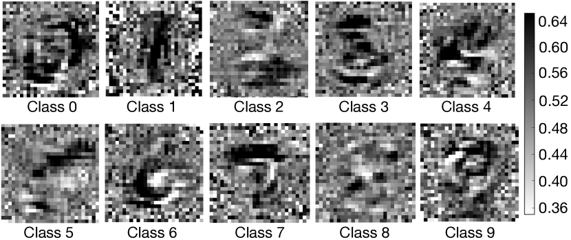
However, we must now complete our analysis to characterize the correlation suggested by the hypothesis testing. In Figure 14, we plot the frequency matrix for several pairs of matrices. The first is a pair of random matrices of . The other matrices correspond to substitute DNN A and the oracle at different substitute training epochs . Frequencies are computed using the samples of the MNIST test set. Although all frequencies in the random pairs are very close to , frequencies corresponding to pixels located in the center of the image are higher in the matrix pairs. The phenomenon amplifies as training progresses through the substitute epochs. We then compute the frequencies separately for each sample source class in Figure 15. Sign matrices agree on pixels relevant for classification in each class. We plotted similar figures for other substitute DNNs. They are not included due to space constraints. They show that substitutes yielding lower transferability also have less components of their cost gradient sign matrix frequently equal to the oracle’s. This suggests that correlations between the respective sign matrices of the substitute DNN and of the oracle—for input components that are relevant to classification in each respective class—could explain cross-model adversarial sample transferability.
C. Discussion of Related Work
Evasion attacks against classifiers were discussed previously. Here, we cover below black-box attacks in more details.
Xu et al. applied a genetic algorithm to evade malware detection [18]. Unlike ours, it accesses probabilities assigned by the classifier to compute genetic variants fitness. These can be concealed by defenders. The attack is also not very efficient: 500 evading variants are found in 6 days. As the classifier is queried heavily, the authors conclude that the attack cannot be used against remote targets. Finally, given the attack’s high cost on low-dimensional random forests and SVMs, it is unlikely the approach would scale to DNNs.
Srndic et al. explored the strategy of training a substitute model to find evading inputs [12]. They do so using labeled data, which is expensive to collect, especially for models like DNNs. In fact, their attack is evaluated only on random forests and an SVM. Furthermore, they exploit a semantic gap between the specific classifiers studied and PDF renderers, which prevents their attack from being applicable to models that do not create such a semantic gap. Finally, they assume knowledge of hand-engineered high-level features whereas we perform attacks on raw inputs.
Tramer et al. considered an adversarial goal different from ours: the one of extracting the exact value of each model parameter. Using partial knowledge of models and equation solving, they demonstrated how an adversary may recover parameters from classifiers hosted by BigML and Amazon [15]. However, it would be difficult to scale up the approach to DNNs in practice. To recover the parameters of a shallow neural network (one hidden layer with neurons) trained on a local machine, they make label queries. Instead, we make label queries to train substitute DNNs made up of hidden layers (each with hundreds of neurons) with a total of over parameters—albeit at the expense of a reduced guaranteed accuracy for the model extraction operation. Unlike theirs, our work also shows that our substitutes enable the adversary to craft adversarial examples that are likely to mislead the remote classifier.